Abstract
As system complexity increases, accurately capturing true system reliability becomes increasingly challenging. Rather than relying on exact analytical solutions, it is often more practical to use approximations based on observed time-to-failure data. Finite mixture models provide a flexible framework for approximating arbitrary probability density functions and are well suited for reliability modelling. A critical factor in achieving accurate approximations is the choice of parameter estimation algorithm. The REBMIX&EM algorithm, implemented in the rebmix R package, generally performs well but struggles when components of the finite mixture model overlap. To address this issue, we revisit key steps of the REBMIX algorithm and propose improvements. With these improvements, we derive parameter estimators for finite mixture models based on three parametric families commonly applied in reliability analysis: lognormal, gamma, and Weibull. We conduct a comprehensive simulation study across four system configurations, using lognormal, gamma, and Weibull distributions with varying parameters as system component time-to-failure distributions. Performance is benchmarked against five widely used R packages for finite mixture modelling. The results confirm that our proposal improves both estimation accuracy and computational efficiency, consistently outperforming existing packages. We also demonstrate that finite mixture models can approximate analytical reliability solutions with fewer components than the actual number of system components. Our proposals are also validated using a practical example from Backblaze hard drive data. All improvements are included in the open-source rebmix R package, with complete source code provided to support the broader adoption of the R programming language in reliability analysis.
Keywords:
system reliability; mixture model; numerical modelling; density estimation; parameter estimation; EM algorithm; REBMIX algorithm MSC:
62-04; 62-08; 62H30
1. Introduction
Estimating system reliability is a complex yet essential task [1,2,3]. It is crucial because system reliability often plays a key role in further analyses, such as calculating the mean time to failure (MTTF) [1,3], determining remaining useful life (RUL) [4], assessing hazard rates [5,6], conducting safety evaluations [7,8], and so on. Accurate reliability estimation enables better decision-making and enhances safety and longevity.
In a complex system consisting of several components, reliability estimation typically involves several steps [9,10]. These include collecting relevant time-to-failure data sets, selecting suitable parametric families for the component time-to-failure distributions, estimating their parameters and finally deriving the overall system reliability model. The application of these steps can be quite challenging even for smaller systems [8]. In addition, in order to obtain meaningful estimates, various assumptions often need to be made that simplify the derivation of the final, more sophisticated reliability models.
On the other hand, surrogate modelling has gained significant popularity for reliability estimation [11,12]. In probabilistic modelling, system reliability is often represented using exponential or Weibull parametric families [5,13]. However, such oversimplifications typically result in poor estimates that are inadequate for complex systems [14,15]. One of the gold-standard methods for reliability estimation is finite mixture modelling [14,16,17,18]. The applicability of finite mixture models (FMMs) for reliability data is well established in the literature, either in the separation of system failure modes [14,19] or component-level heterogeneity [16,17,18]. Additionally, this semi-parametric approach is capable of modelling a wide range of random phenomena beyond reliability data [20,21,22,23,24]. While FMMs are a part of probabilistic modelling, their inherent properties also make them useful for uncovering additional meaningful insights about the systems being analysed [14,19].
Despite significant progress, the development of a suitable parameter estimation algorithm for different FMMs remains elusive. Research on normal FMMs, where the normal parametric family serves as the component distribution, is abundant and includes well-established parameter estimation algorithms along with software implementations [25]. In contrast, similar studies addressing FMMs with alternative parametric families, such as lognormal, gamma, or Weibull, are lacking, likely due to their limited use and the practical difficulties associated with their derivation and implementation [26,27,28]. Nonetheless, these parametric families are particularly relevant in reliability analysis, as they often provide a better fit for modelling the time-to-failure distributions of system components [16,29,30,31]. Furthermore, readily available software implementations of these FMMs are often lacking or, at the very least, remain unknown to the wider public. Addressing this gap is essential for the wider adoption of FMMs in practical reliability studies, particularly where the flexibility to incorporate diverse parametric families as component distributions is critical for accurately capturing system behaviour.
The Expectation–Maximisation (EM) algorithm is widely considered the most promising approach in terms of accuracy and computational efficiency for estimating parameters in FMMs [18]. However, since the EM algorithm requires proper initialisation, recent studies have highlighted that the Rough-Enhanced-Bayes (REBMIX) algorithm can also effectively tackle this issue, albeit with certain limitations [25,32]. More specifically, recent findings in [25] suggest that REBMIX struggles when components in the FMM are highly overlapping. To address these challenges, we briefly review the REBMIX algorithm and propose improvements to its rough component parameter estimation and Bayesian mixture parameter optimisation steps. Furthermore, we derive comprehensive parameter estimation formulas for both the EM and REBMIX algorithms for lognormal, Weibull, and gamma parametric families, and we provide ready-to-use software implementations within the rebmix R package. We also review other popular R packages that can be used to estimate parameters of lognormal, Weibull, and gamma FMMs. All corresponding source code is included as Supplementary Material to ensure full reproducibility of this work.
Finally, to obtain conclusive benchmarks, we designed a comprehensive simulation study involving four different system configurations. For each configuration, the exact system reliability and corresponding probability density function were analytically derived. The lognormal, gamma, and Weibull parametric families were used to model the time-to-failure distributions of individual system components. The parameters for each component’s distribution were generated to ensure significant overlap between them. This process was repeated for 20 different random seeds to thoroughly evaluate: (a) the performance of the improved REBMIX&EM parameter estimation algorithm, (b) its benchmarking against state-of-the-art estimation methods implemented in freely available R packages, and (c) the effectiveness of different FMMs in approximating the true system reliability.
The remainder of this paper is organized as follows. Section 2 presents all the improvements made to the parameter estimation procedures. Section 3 outlines the simulations. Section 4 discusses the results, while Section 5 gives the practical real-life example. Section 6 provides the concluding remarks. Appendix A contain the derivations of the EM and REBMIX parameter estimation methods for the lognormal, Weibull and gamma FMMs.
2. Methodology
In this section, recent improvements to the REBMIX algorithm are presented, mainly inspired by the findings in [25]. Chassagnol et al. [25] demonstrated that REBMIX initialisation provides the most accurate estimates when working with well-separated components or a small number of components with clearly distinguishable modes. Furthermore, the study indicated that for data sets with highly overlapping components, k-means [33] or random initialisation [34] gives more accurate results. The advances presented in this article are intended to demonstrate improved performance in cases with moderately overlapping components as well as increased accuracy and calculation speed. The scope of this study is restricted to lognormal, Weibull and gamma FMMs.
2.1. Lognormal, Weibull and Gamma FMMs
Let be an observed dimensional data set of size n of continuous observations. Each observation is assumed to follow the predictive FMM density
The objective of the analysis is to obtain the number of components c, the component weights , which sum to 1, and the component parameters . It is assumed that the component time-to-failure probability densities come from the lognormal
Weibull
gamma
parametric family.
2.2. Parameter Estimation
The REBMIX algorithm [35] was originally developed as a sequential method in which the components are estimated individually. The algorithm is composed of several steps, which are shown in Figure 1. However, a significant limitation is the inability to reach the optimal solution. Thus, recent studies [32] propose to merge the algorithm with the EM algorithm [36] to form REBMIX&EM.
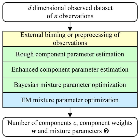
Figure 1.
Flowchart of REBMIX&EM.
In this case, REBMIX first provides estimates for the number of components c, the weights and the parameters , which are usually close to the optimum. The EM algorithm then refines these estimates to converge to the optimal solution.
Nevertheless, the introduction of the EM algorithm into the estimation procedure did not solve the problems of optimising the spurious optima with overlapping components in the FMM. We have found that the main problems lie in the rough parameter estimation step and the Bayesian mixture parameter optimisation step, which we will discuss in more detail in the following text.
2.2.1. Rough Parameter Estimation
The rough parameter estimation phase is the most important step in the REBMIX algorithm. In this phase, rough parameters for the lth component are estimated based on the global mode position and its probability density . These parameters are then used to cluster observations between the lth component and the residue, as detailed in [35,37]. Unlike algorithms such as k-means, which depends exclusively on the positions of observations and their distances, REBMIX utilizes additional information from the data set. It not only considers the positions of observations but also identifies the global mode, a distinctive feature of the data set. The determination of the empirical densities by histogram preprocessing or external binning of the observations into nonempty bins also substantially reduces computational time, especially for large data sets. For small data sets, kernel density estimation or k-nearest neighbour may be preferable for preprocessing the observations.
However, a fundamental problem, illustrated in Figure 2, remains unresolved. Figure 2 presents three plots, where rough component parameter estimation is depicted on three different estimation cases, namely a FMM with non-overlapping components (the plot on the left), moderately (the middle plot) and heavy overlapping components (the plot on the right). In all three plots, the residue is shown in green, the lth component in red and the FMM probability density as a black line. The global mode is indicated by a black circle, while the mode of the true lth component is indicated by a red circle. The true residue probability density at the global mode is shown by a green circle. The left and right global minima are represented by a black triangle pointing upwards and a triangle pointing downwards, respectively. The rough probability density of the lth component is depicted by a thin red solid line, and the loose probability density of the lth component is shown by a thin blue line.
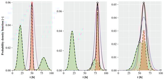
Figure 2.
Rough component parameter estimation. The left plot shows the FMM estimation problem with non-overlapping components. The middle plot shows the FMM estimation problem with moderately overlapping components, and the right plot shows the estimation problem with heavily overlapping components of the FMM.
The empirical density of the global mode belongs exclusively to the lth component only if the components are well separated (see red circle in left plot of Figure 2), which overlaps the black circle. This is generally not the case for moderately or heavily overlapping components, as shown in the middle and right plots of Figure 2. In these cases, the red and black circles are misaligned. The approach proposed in [38], which is implemented in the package rebmix version 2.15.0 and older remains accurate only under conditions where components are well separated, as shown in the left plot of the Figure 2, or if a single component of the residue contributes to , as shown in the middle plot of the Figure 2. Cases where multiple components contribute to the lth component, as illustrated in the right plot of the Figure 2, may lead to estimation errors in . According to [38], the wider component of the residue in the middle plot of the Figure 2 (mean , standard deviation ) is extracted before the dominant lth narrower component (, ), which is suboptimal. Ideally, the dominant component in red, centred on , should be extracted first. The refined rough parameter estimation, which addresses the the aforementioned issues, is outlined below.
After preprocessing or external binning of observations, the empirical probability densities (black solid line) are obtained, from which the global mode position and the corresponding value can be readily identified. The true component probability density , marked by the red circle, and the true probability density of the residue
marked by the green circle, are not available at this stage. Assume that the weight of the lth component is and that . In other words, the thin red line representing the envelope under which the entire lth component is believed to be contained can be calculated and visualised. The component parameters of the red thin lines in Figure 2 were connected to rigid restraints for the first time in [38]. It was further demonstrated in [38] that the rigid restraints alone are not sufficient to accurately restore the components of the residue when they overlap. Furthermore, an iterative procedure for defining the rough component parameters based on loose restraints was proposed in [38].
If we carefully observe the area between the red thin lines and the black lines in Figure 2, we can see that there is a global minimum (triangle pointing upwards) to the left of and another (triangle pointing downwards) to the right of the global mode. At the beginning let or equivalently . Then
The sum of the differences between the empirical densities and the corresponding probability densities of the lth component
is also calculated, where h stands for the bin widths. Next, the number and the density are both initialised to zero. If and , is incremented and is increased by . Similarly, if and , and . Finally, if , . The loose restraints then lead to
from which the loose rough component parameters, , are calculated as explained in Appendix A.1. For simpler notation, let and . In Figure 2, the probability densities of the lth component associated with the loose restraints are shown as thin blue lines.
Equation (8) is valid only for non-overlapping bins. For kernel density estimation, the histogram is constructed with one bin aligned with . Similarly, for k-nearest neighbour, the histogram is constructed with one bin aligned with . Here, , where denotes the mean Euclidean distance to the first non-coincident nearest neighbour. Further details on the estimation of the rough component parameters can be found in [35,37].
2.2.2. Bayesian Mixture Parameter Optimisation
The REBMIX algorithm clusters an observed data set of size n into c clusters of sizes associated with component probability densities and component weights . The clustering is designed to minimise both the sum of the positive relative deviations and the information criterion. As a result, the sum of the component weights satisfies , meaning that some observations may remain unassigned.
At the beginning, the number of outliers N is set to zero and the initial first moments and second moments are taken from Appendix A.3. The remaining observations are then allocated to the existing components based on the Bayes decision rule
For each observation, it is also determined whether it is an outlier. Outliers are identified as those that fall into the left or right tail of the probability density with a probability of . If the observation is recognised as an outlier, then . Otherwise
This ensures that the outliers do not influence and . A detailed explanation of the frequencies associated with the densities can be found in [35].
After processing v bins or n observations, depending on the type of preprocessing, the component weights are recalculated
to fulfil . The initial FMM parameters for the EM are finally obtained by inverting Equations (A22)–(A27). The lognormal parameters result from
The Weibull parameters are a solution of
To avoid numerical problems, the minimum value of was set to . If Equation (17) returns a value less than or equal to zero, then is set to . Otherwise, is used as the initial estimate. The gamma parameters are given by
This section introduces an important improvement with the inclusion of outliers, as compared to [14].
3. Simulations
To demonstrate the improvements of improved rough component parameter estimation and enhanced Bayes classification of unassigned observations, the R package rebmix [37] (version 2.16.0) was compared to five widely used alternatives: flexmix [39,40] (version 2.3-20), ltmix [41] (version 0.2.2), mixdist [42] (version 0.5-5), mixR [43] (version 0.2.1), and mixtools [44,45] (version 2.0.0.1. The comparison focused on three common parametric families in the reliability domain: lognormal, Weibull and gamma. In addition, four system configurations, as shown in Figure 3, were analysed. To cover a wide range of sample sizes, data sets with 50, 100, 500 and 1000 observations were used. The parameters for the probability density functions were generated using random seeds ranging from 1 to 20.
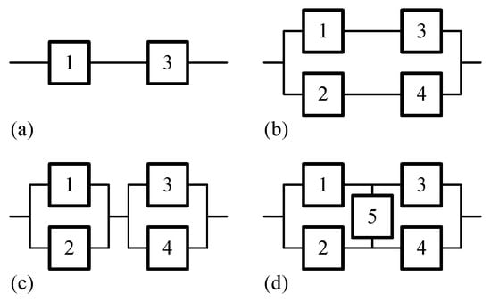
Figure 3.
Block diagram: (a) serial system, (b) high-level redundant system, (c) low-level redundant system, and (d) linked system.
The Weibull and gamma parameters were simulated according to the following equations
where denotes a uniform distribution in the range . The lognormal distribution parameters were simulated as
Here, the index l stands for the number of the component, . Each package was thus evaluated on well distinguishable data sets.
The R packages were evaluated according to the Bayesian Information Criterion (BIC) and the calculation time. The BIC is commonly regarded as the standard information criterion to assess how well the estimated FMM fits a data set.
On the other hand, the calculation time is of key importance when numerous data sets or large data sets have to be processed. This is particularly important as FMMs are often associated with solving complex regression, clustering, classification or other data mining tasks.
All of the aforementioned packages are based on the EM algorithm, although they use different strategies to determine the initial set of FMM parameters. We also performed initial tests with the package ForestFit (version 2.4.3) [46], which was significantly slower than the others. Considering the computational challenges of processing 960 data sets within a reasonable time frame, ForestFit was not further evaluated.
Assuming that the time-to-failure probability densities and the corresponding reliabilities of the five components in Figure 3 are known, the exact system reliability for the linked system configuration (d) can be expressed as follows
For the sake of simplicity, the dependency on the variable t is omitted from the notation. The exact system time-to-failure probability density for the linked system configuration (d) is then
If and , then the last two equations correspond to the low-level redundant system configuration (c). High-level redundant system configuration (b) is obtained when and . Serial system configuration (a) is achieved if and for .
Although the systems under consideration consist of no more than five components, Equations (25) and (26) are already quite complex. For systems with a large number of components, it is no longer feasible to derive analytical equivalents for these equations. In addition, the structure of Equation (26) differs significantly from that of Equation (1). Nevertheless, it is possible to show that the FMM is an excellent and compact approximation to the exact system time-to-failure probability density.
Figure 4 illustrates the time-to-failure probability densities for components 1 to 5, which are colour-coded as follows: Component 1 in red, 2 in green, 3 in blue, 4 in cyan and 5 in purple. The components have significantly different times to failure. The exact time-to-failure probability density of the system, shown in black, shows two different modes. The first mode lies between the modes of components 1 and 3, while the second mode closely matches the mode of component 2. Figure 5 also shows that components 4 and 5 do not contribute significantly to the reliability of the system.
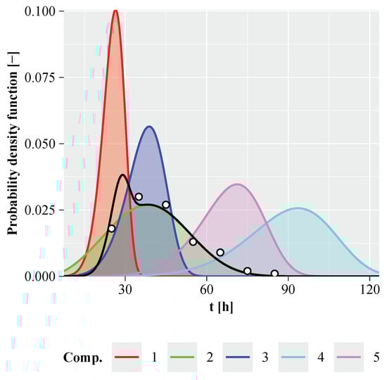
Figure 4.
Weibull component probability densities for the linked system, with the exact system time-to-failure probability density shown by the black line and the Monte Carlo simulated sample represented by circles. Parameters: , , .
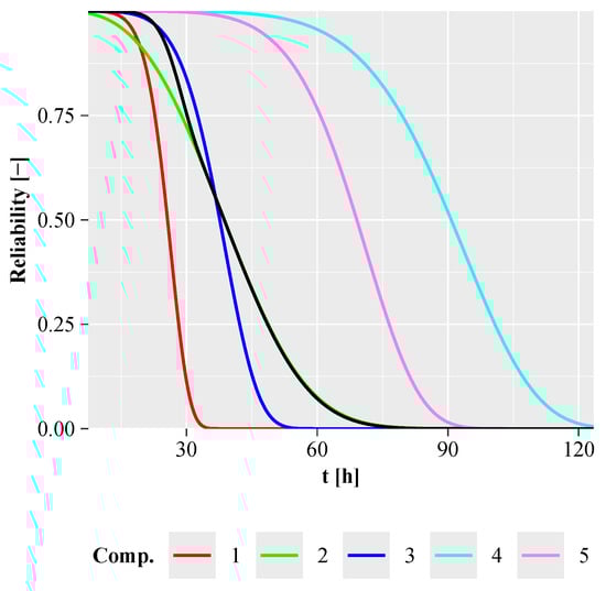
Figure 5.
Weibull component reliabilities for the linked system, with the exact system reliability shown by the black line. Parameters: , , .
The times to system failure were randomly generated using Monte Carlo simulation, based on the known time-to-failure probability densities of the individual components. In order to take different system configurations into account, each component was assigned an indicator . Specifically, indicates that , means that , and represents . The times to failure of the component l were generated for the parametric Weibull family as follows
The function of the random number generator used to model the times to failure is either , or . The different system configuration, illustrated in Figure 3, is thus uniquely defined by an indicator array , where is the lth system component indicator variable as described in the paragraph above. For example, the indicator array for a low-level redundant system, illustrated in Figure 3c, is and the indicator array for a linked system, illustrated in Figure 3d, is . Finally, the time until system failure is then given by
In other words, the time to system failure depends on the four minimal paths of the system. In this way, data sets of different lengths were created. The pseudo code for data set generation is given in Algorithm 1.
The R files flexmix.R, ltmix.R, mixdist.R, mixR.R, mixtools.R and rebmix.R are provided as Supplementary Materials to enable the reproduction of all results presented in this article. Please replace the working directory setwd() and make sure that the required packages are installed before executing the above *.R files. The R programming environment has undoubtedly become the leading platform for statistical computing. Figures such as Figure 4 and Figure 5 can be reproduced by running the figures.R script.
| Algorithm 1: System time-to-failure data set generation. |
|
4. Results and Discussion
The package rebmix was developed for FMM parameter estimation, with a particular focus on large data sets and the Weibull parametric family [35,38]. It is primarily characterized by its distinctive approach of sequential rough parameter estimation, which significantly reduces computational time relative to other EM-based packages. In contrast, where these alternatives rely on simultaneous parameter estimation and require initial estimates for all parameters, rebmix achieves greater efficiency through its streamlined process.
However, a major disadvantage of rebmix was its lower accuracy, as indicated by higher values for the information criteria, where other packages performed better. To address this limitation, an EM step was incorporated [32] to fine-tune the FMM parameters. Although this improvement reduced computational speed, it enhanced accuracy. The effects of the latest improvements to the package are demonstrated below. The computational procedure for obtaining the results presented in this section and for further analysis is shown in Figure 6.
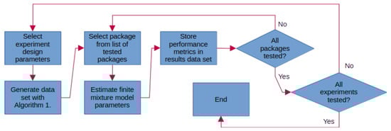
Figure 6.
Procedure used for obtaining data for result analysis.
The 960 data sets were initially processed by all six packages. Since the system is composed of five components, the optimal solution was searched for to 5, where c is the number of components. The package rebmix offers three types of preprocessing: histogram, kernel density estimation (KDE) and k-nearest neighbour (KNN). Histogram preprocessing is particularly suitable for larger data sets, while KDE and KNN are more suitable for smaller data sets. The KDE&histogram option in Table 1 indicates that the histogram preprocessing was used if the number of observations , otherwise KDE was used. The package rebmix provided the most favourable BIC values. The rebmix can also use a histogram as input by first converting the data set using the methods fhistogram or chistogram. See rebmix help for details. This option is referred to as binned in the table.

Table 1.
Comparison of packages for different preprocessing based on mean BIC (bold values represent the best values obtained).
As can be seen from Table 2, the package rebmix was on average 241 times faster than flexmix and 1029 times faster than mixtools. For further analysis, we chose the binned option, which resulted in an average BIC that was lower than that of the second-best package ltmix. Details on how to use this option can be found in the file rebmix.R.
Table 2.
Comparison of packages for different preprocessing based on mean calculation time [s] (bold values represent the best values obtained).
Studying the mean values alone is insufficient. For Table 3 and Table 4, the values of and were calculated for all 960 data sets, where . The summation was performed as follows: for , a value of one was added; for a value of minus one was added; and for zero was added to the sum. This process was carried out separately for each parametric family. The same logic was applied to .
Table 3.
Comparison of rebmix using binned input with other packages for different parametric families based on (bold values represent the best values obtained).
Table 4.
Comparison of rebmix using binned input with other packages for different parametric families based on (bold values represent the best values obtained).
The values in the tables can range from − 320 to 320, with a positive value indicating that rebmix outperformed package p. It is obvious that the improved REBMIX&EM algorithm not only worked faster, but also provided better BIC estimates compared to the other packages. For the gamma parametric family, however, ltmix flexmix, mixR and mixtools performed slightly better. In terms of speed, rebmix was faster in almost all cases. The NA entries in the tables indicate that mixtools could not process the lognormal and Weibull parametric families.
Next, the effects of the parametric family and the sample size on the BIC and the calculation time were analysed. The Table 5 and Table 6 show the mean values and standard deviations (in brackets) for the information criterion and the calculation time. In terms of BIC, rebmix performed best in seven cells of Table 5, followed by ltmix, which performed best in six cells, and mixR, which performed best in four cells. The other packages only achieved the best BIC in one cell. In terms of calculation time, rebmix performed better than all other packages in all cells of Table 6.
Table 5.
Comparison of packages for different parametric families and sample sizes based on mean BIC (bold values represent the best values obtained).
Table 6.
Comparison of packages for different parametric families and sample sizes based on mean calculation time [s] (bold values represent the best values obtained).
To summarise, the accuracy of the rebmix package has improved significantly compared to its previous versions, while maintaining its superiority in calculation time. This progress is particularly important as it increases the potential of rebmix, not only for FMM parameter estimation, but also for applications in image segmentation [32] and in combination with neural networks for image processing.
The effect of packages on different parametric families was analysed based on the estimated optimal number of components. As shown in Figure 7, the FMM in the case of mixdist includes only one component in 796 out of 960 cases (). This indicates that, although the systems may consist of up to five components, a single-component FMM is sufficient to reliably represent the system in of cases, despite the variability in component time-to-failure probability densities shown in Figure 8 and Figure 9. Two components were required in of cases, three components in , four components in and five components in only of cases.
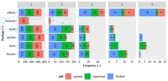
Figure 7.
Comparison of packages for different parametric families based on the number of components.
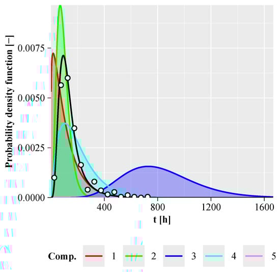
Figure 8.
Gamma component probability densities for the low-level redundant configuration, with the exact system probability density shown by the black line and the Monte Carlo simulated sample represented by circles. Parameters: , , .
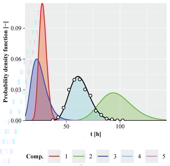
Figure 9.
Lognormal component probability densities for the high-level redundant configuration, with the exact system probability density shown by the black line and the Monte Carlo simulated sample represented by circles. Parameters: , , .
This result indicates that the complexity of the FMM does not necessarily increase with the increasing complexity of the system. However, the complexity of the exact system reliability increases with the complexity of the system. This supports the hypothesis that the FMM is an excellent approximation of the exact system reliability function, as it allows a very compact formulation of the system reliability and the system time-to-failure probability density. All tables and figures in this section can be reproduced by executing the file tables.R.
5. Practical Example
To demonstrate the practical usefulness of our proposed approach, we utilized hard disk drive (HDD) and solid-state drive (SSD) data from the Backblaze data center [47]. The time-to-failure data was extracted from the 2024 Q4 data set, spanning the period from 1 October to 31 December 2024. For each day within this period, a snapshot was available containing information on both operational and failed HDDs and SSDs. We identified all drives that failed on a given day and extracted their power-on hours, represented by the S.M.A.R.T. 9 attribute [48], as a proxy for time-to-failure. Using this method, we compiled a total of 1030 time-to-failure data points from HDDs and SSDs that failed during Q4 2024. A histogram illustrating the distribution of these time-to-failure values is shown in Figure 10.
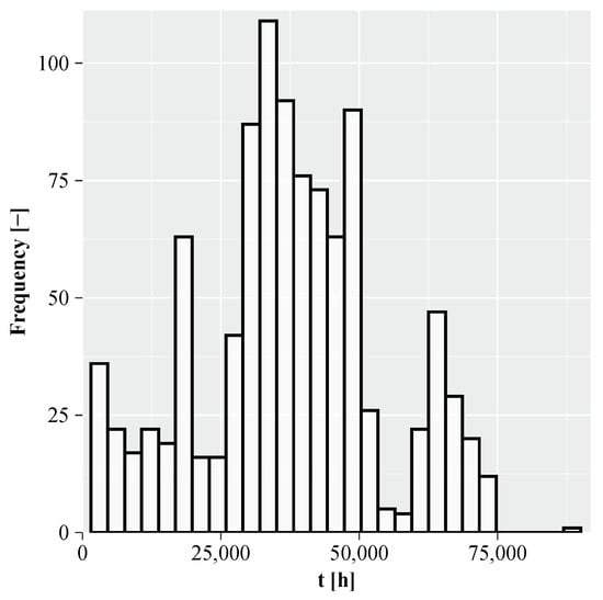
Figure 10.
Histogram of Backblaze HDDs and SSDs time-to-failure data set.
All packages, namely rebmix, flexmix, ltmix, mixdist, mixR, and mixtools, used in the simulation study were also applied here to estimate the parameters of the FMMs. For flexmix, ltmix, mixdist, mixR, and mixtools, we used the same package-specific settings as before. In the case of rebmix, we selected only the histogram preprocessing method, as it yielded the fastest and most accurate results. Table 7 reports the BIC values of the FMMs estimated using different packages, and Table 8 presents the corresponding computation times. Additionally, Table 7 reports the number of components estimated in the FMMs for each package and parametric family, indicated in parentheses next to the corresponding BIC value.
Table 7.
BIC values and corresponding estimated number of components in the FMMs for different packages and parametric families (bold values represent the best values obtained).
Table 8.
Computation times across different packages and parametric families (bold values represent the best values obtained).
Since the parametric family is not known a priori for the presented data set, we applied all three parametric families explored in this study: Weibull, gamma, and lognormal. As shown in Table 7, the majority of packages achieved their best BIC values with the gamma FMM, with the exception of mixR, which yielded a lower BIC for the lognormal FMM. Additionally, regardless of the chosen parametric family, most packages consistently estimated FMMs with five components as the most suitable model. The best-performing gamma FMM, based on the observed BIC values, was estimated using the rebmix package, which also provided the overall best estimate. The top Weibull and lognormal FMMs were estimated using mixR and rebmix, respectively. The best-fitting Weibull, gamma, and lognormal FMMs are visualized in Figure 11. Finally, in terms of computational efficiency, the rebmix package clearly outperformed all others, with mixR being the second fastest, although it was, on average, five times slower than rebmix.
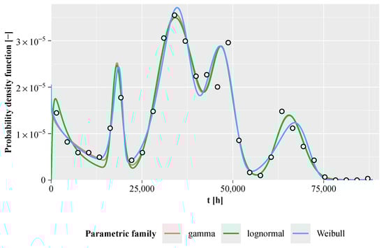
Figure 11.
Probability density function estimates of the best-performing FMMs for different parametric families. Points represent the corresponding histogram estimates.
6. Conclusions
This article tackles several open challenges related to the use of FMMs in reliability studies. First, we addressed the shortcomings of the REBMIX&EM parameter estimation algorithm. Second, we demonstrated the advantages of using lognormal, Weibull, and gamma FMMs to approximate system reliability, and derived all associated parameter estimation equations. Our third objective was to promote the use of the R Project for Statistical Computing [49] in the fields of reliability, maintainability, and supportability. To that end, we evaluated six R packages relevant to these domains. All evaluated packages are applicable to reliability modelling, and all but one offer straightforward usage. The mixtools package currently supports only the gamma parametric family. In contrast, the mixdist package requires additional programming effort, as it lacks built-in functionality for estimating initial parameters. To address this, we used the kmeans algorithm [49] to initialize parameter values. We have also provided all accompanying source code to enable full reproducibility and to serve as a starting point for further research.
To demonstrate the improvements to the REBMIX&EM parameter estimation algorithm implemented in rebmix R package the serial system, the high-level redundant system, the low-level redundant system and the linked system were analysed. Four different sample sizes and three parametric families were studied. The data sets were simulated across a wide range of parameters defining the component time-to-failure distributions. A total of 960 data sets were processed with each package. The findings of the article can be summarised as follows:
- The number of components of the FMM is usually lower than the number of components from which the system is composed.
- The lognormal, Weibull and gamma parametric families are all suitable for modelling system reliability. However, it is impossible to determine the best family in advance. Therefore, it is recommended to estimate the FMM parameters for each family and choose the one that yields the lowest information criterion.
- The BIC is the most preferred and widely used information criterion.
- The improved rough component parameter estimation and enhanced Bayes classification of unassigned observations have significantly increased the calculation speed of the REBMIX algorithm.
- The improved REBMIX&EM algorithm has improved the accuracy of estimating the parameters of a FMM, at least for univariate problems. REBMIX is used here to determine the initial parameters for the EM algorithm.
- All calculations of the article can be reproduced via supplementary *.R files in the R programming environment.
Based on the results of the simulation study, the rebmix R package provides very fast and accurate FMM estimates. The mixR package also demonstrated competitive performance. The flexmix and ltmix packages showed similar performance levels and offer extensive feature sets within their respective domains. In contrast, the mixdist package was the least user-friendly, as it requires manual specification of initial FMM parameters. Additionally, the mixtools package currently lacks support for the Weibull and lognormal parametric families.
We also analysed a practical case study involving time-to-failure data from Backblaze hard drives. In this analysis, all packages used in the simulation study were applied for FMM parameter estimation. The best overall FMM, based on BIC, was a gamma FMM with five components, estimated using the rebmix package. Both the rebmix and mixR packages produced the best estimates for the Weibull and lognormal FMMs. As in the simulation study, rebmix achieved the shortest computation time, while mixR again showed strong and competitive performance.
The rebmix package, with the improved REBMIX&EM parameter estimation algorithm presented in this study, offers highly competitive performance, delivering accurate estimates with minimal computation time. However, because the REBMIX algorithm is deterministic, it always produces the same initial parameters for the EM algorithm, unlike random initialisation, which can eventually outperform deterministic approaches given enough time. Packages like flexmix and ltmix, which use random initialisation, can explore the parameter space more broadly and eventually lead to more accurate estimates, or at least equivalent ones, if no better solution exists than that found by deterministic approach. The mixR package uses k-means for initialisation, a middle ground between deterministic and random approaches. While k-means is more efficient than random initialisation and often effective for normal FMMs, it may miss optimal solutions due to its assumption of spherical clusters for non-normal FMMs. Nonetheless, in our study, mixR provided good FMM estimates, confirming the practical value of k-means in this context.
To summarise, with recent improvements, the REBMIX algorithm has become more competitive for non-overlapping and moderately overlapping FMMs. Our future work will focus on enhancing REBMIX’s performance in highly overlapping scenarios, where k-means and random initialisation methods still lead the field [25]. We also plan to investigate kernel density estimation preprocessing within the REBMIX framework more deeply. The current implementation in the rebmix package uses radial basis function kernels, with the bandwidth either specified by the user or selected through an iterative search based on the chosen information criterion, such as BIC. Future research should explore alternative kernel types and develop more robust bandwidth selection strategies. Finally, this study opens several directions for further advancement in statistical analysis. The improved REBMIX&EM algorithm could be extended to support more complex parametric families, and adapted for use with multivariate reliability data, time-varying covariates, or censored observations. These features are commonly encountered in industrial systems.
Supplementary Materials
The following supporting information can be downloaded at: https://www.mdpi.com/article/10.3390/math13101605/s1.
Author Contributions
Conceptualization, M.N., S.O., J.K. and B.P.; methodology, M.N., S.O., J.K. and B.P.; software, M.N.; validation, M.N., S.O., J.K. and B.P.; formal analysis, M.N.; investigation, M.N., S.O., J.K. and B.P.; resources, M.N., S.O., J.K. and B.P.; writing—original draft preparation, M.N., S.O., J.K. and B.P.; visualization, M.N., S.O., J.K. and B.P.; supervision, M.N., S.O., J.K. and B.P.; funding acquisition, M.N. and J.K. All authors have read and agreed to the published version of the manuscript.
Funding
The authors acknowledge financial support from the Slovenian Research and Innovation Agency (research core funding No. P2-0182 entitled Development Evaluation).
Data Availability Statement
The original contributions presented in this study are included in the article/Supplementary Materials. Further inquiries can be directed to the corresponding author.
Conflicts of Interest
The authors declare no conflicts of interest.
Appendix A
Appendix A.1. Rough Component Parameters
The rough component parameters [35] are derived by the optimisation method of Lagrange multiplier
which provides a strategy for entropy maximisation subject to the logarithm of (2), (3) or (4). The rough lognormal component parameters can therefore be determined numerically by solving the following equation
where
Equation (A2) has no solution within the range . If left hand side of Equation (A2) is positive for small positive number (e.g., ), then it is assumed that the solution is . Otherwise, is used as an initial guess for root finding methods such as Newton–Raphson.
Similarly, the rough Weibull component parameters can be determined by solving
with
To avoid numerical problems, the minimum value of was set to , which corresponds to . If Equation (A5) returns a value greater than or equal to zero, then is set to . Otherwise, is used as the initial estimate, which corresponds to the maximum of left hand side expression of Equation (A5). The optimum value of is then determined using a root-finding method.
Finally, the rough gamma component parameters result from
with
The minimum value of is also set here to , which corresponds to . If left hand side expression of Equation (A10) returns a value less than or equal to zero, then . Otherwise, the initial estimate for . Then the root finding takes place as above. Equations (A10) and (A11) were derived by approximating the digamma function as . In addition, the logarithm of the gamma function was approximated using Stirling’s approximation, . For more details on the global mode position and its empirical density see Ref. [35]. The estimation of the rough component parameters is robust and not susceptible to numerical instability.
Appendix A.2. Enhanced Component Parameters
Maximum likelihood estimation (MLE) is employed to obtain enhanced component parameters. This is achieved by maximising the likelihood function
The enhanced lognormal component parameters for the kernel density estimation and the k-nearest neighbour can be derived as follows
Similarly, enhanced Weibull component parameters yield from
Finally, the enhanced gamma component parameters are obtained by applying a root-finding method to
If the index number of observations n is replaced by the number of bins v and by , the equations of this section are also valid for the histogram preprocessing. For further details, e.g., on the frequencies and the number of observations in the class l, see [35].
The estimation of the enhanced component parameters can be unstable, which can lead to one or more component densities approaching singularity. To check whether a singularity exists, the variances for the rough and the enhanced component parameters are calculated. If , the rough component parameters are regarded as the enhanced component parameters. The variance multiplier is set to in rebmix.
Appendix A.3. First and Second Moment Calculation
Immediately after estimating the enhanced component parameters, the first moment and the second moment are calculated. For the lognormal parametric family, these are given by
For the Weibull parametric family, we have
and for the gamma parametric family
These values serve as initial estimates for the Bayesian mixture parameter optimisation.
Appendix A.4. EM Mixture Parameters
The EM algorithm is composed of two key steps: the Expectation (E) step and the Maximisation (M) step. During the E step, the posterior probabilities are calculated as follows
for , where t denotes the current iteration number. During the M step, the parameters are updated by maximising the complete data log-likelihood, as outlined in [18]. Consequently, the component weight is given by
The lognormal parameters are computed as
The Weibull parameters are determined as
Finally, the gamma parameters are given by
The equations in Appendix A are implemented in the rebmix package exactly as presented. However, we found that, for instance, modifying Equation (A32) for by dividing it with a factor of can result in a slightly different estimate for than when solved as originally written. We believe that this discrepancy arises from the accumulation of numerical errors that occur in mathematical operations with very small numbers.
The initial parameter set for the EM algorithm is derived from the Bayesian mixture parameter optimisation. If the EM parameter estimation fails due to problems such as singularities, REBMIX&EM still provides a finite set of FMM parameters based on Bayesian optimisation, which is not susceptible to numerical problems.
References
- Ramezani, R.; Clemente, J.A.; Franco, F.J. Analytical reliability estimation of SRAM-based FPGA designs against single-bit and multiple-cell upsets. Reliab. Eng. Syst. Saf. 2020, 202, 107036. [Google Scholar] [CrossRef]
- Rentong, C.; Zhang, C.; Shaoping, W.; Yujie, Q. Reliability estimation of mechanical seals based on bivariate dependence analysis and considering model uncertainty. Chin. J. Aeronaut. 2021, 34, 554–572. [Google Scholar] [CrossRef]
- Yamamoto, A.Y.; Ababei, C. Unified reliability estimation and management of NoC based chip multiprocessors. Microprocess Microsyst. 2014, 38, 53–63. [Google Scholar] [CrossRef]
- Davila-Frias, A.; Yodo, N.; Le, T.; Yadav, O.P. A deep neural network and Bayesian method based framework for all-terminal network reliability estimation considering degradation. Reliab. Eng. Syst. Saf. 2023, 229, 108881. [Google Scholar] [CrossRef]
- Zhu, T. Reliability estimation for two-parameter Weibull distribution under block censoring. Reliab. Eng. Syst. Saf. 2020, 203, 107071. [Google Scholar] [CrossRef]
- Kumari, R.; Tripathi, Y.M.; Sinha, R.K.; Wang, L. Reliability estimation for bathtub-shaped distribution under block progressive censoring. Math. Comput. Simul. 2023, 213, 237–260. [Google Scholar] [CrossRef]
- Ding, C.; Wei, P.; Shi, Y.; Liu, J.; Broggi, M.; Beer, M. Sampling and active learning methods for network reliability estimation using K-terminal spanning tree. Reliab. Eng. Syst. Saf. 2024, 250, 110309. [Google Scholar] [CrossRef]
- Wang, J.; Meng, B.; Zhang, L.; Yu, C. Degradation modeling and reliability estimation for mechanical transmission mechanism considering the clearance between kinematic pairs. Reliab. Eng. Syst. Saf. 2024, 247, 110093. [Google Scholar] [CrossRef]
- Liu, D.; Wang, S. Reliability estimation from lifetime testing data and degradation testing data with measurement error based on evidential variable and Wiener process. Reliab. Eng. Syst. Saf. 2021, 205, 107231. [Google Scholar] [CrossRef]
- Ma, Z.; Wang, S.; Ruiz, C.; Zhang, C.; Liao, H.; Pohl, E. Reliability estimation from two types of accelerated testing data considering measurement error. Reliab. Eng. Syst. Saf. 2020, 193, 106610. [Google Scholar] [CrossRef]
- Teng, D.; Feng, Y.W.; Lu, C.; Keshtegar, B.; Xue, X.F. Generative adversarial surrogate modeling framework for aerospace engineering structural system reliability design. Aerosp. Sci. Technol. 2024, 144, 108781. [Google Scholar] [CrossRef]
- Chen, J.; Chen, Z.; Jiang, W.; Guo, H.; Chen, L. A Reliability-Based Design Optimization Strategy Using Quantile Surrogates by Improved PC-Kriging. Reliab. Eng. Syst. Saf. 2024, 253, 110491. [Google Scholar] [CrossRef]
- Charruau, S.; Guerin, F.; Dominguez, J.H.; Berthon, J. Reliability estimation of aeronautic component by accelerated tests. Microelectron. Reliab. 2006, 46, 1451–1457. [Google Scholar] [CrossRef]
- Nagode, M.; Oman, S.; Klemenc, J.; Panić, B. Gumbel mixture modelling for multiple failure data. Reliab. Eng. Syst. Saf. 2023, 230, 108946. [Google Scholar] [CrossRef]
- Li, M.; Wang, Z. Surrogate model uncertainty quantification for reliability-based design optimization. Reliab. Eng. Syst. Saf. 2019, 192, 106432. [Google Scholar] [CrossRef]
- Jiang, R.; Zuo, M.; Li, H.X. Weibull and inverse Weibull mixture models allowing negative weights. Reliab. Eng. Syst. Saf. 1999, 66, 227–234. [Google Scholar] [CrossRef]
- Jiang, R.; Murthy, D.; Ji, P. Models involving two inverse Weibull distributions. Reliab. Eng. Syst. Saf. 2001, 73, 73–81. [Google Scholar] [CrossRef]
- McLachlan, G.; Peel, D. Finite Mixture Models; Wiley Series in Probability and Statistics: New York, NY, USA, 2000. [Google Scholar]
- Puppo, L.; Pedroni, N.; Di Maio, F.; Bersano, A.; Bertani, C.; Zio, E. A Framework based on Finite Mixture Models and Adaptive Kriging for Characterizing Non-Smooth and Multimodal Failure Regions in a Nuclear Passive Safety System. Reliab. Eng. Syst. Saf. 2021, 216, 107963. [Google Scholar] [CrossRef]
- Li, M.; Wang, Z. Heterogeneous uncertainty quantification using Bayesian inference for simulation-based design optimization. Struct. Saf. 2020, 85, 101954. [Google Scholar] [CrossRef]
- Hu, W.; Qian, Q. Small data reliability analysis in concrete three-point bending tests: A Weibull mixture model approach based on Weibull fracture theory. Eng. Fract. Mech. 2024, 309, 110344. [Google Scholar] [CrossRef]
- Jia, D.W.; Wu, Z.Y. Structural reliability analysis under stochastic seismic excitations and multidimensional limit state based on gamma mixture model and copula function. Probabilistic Eng. Mech. 2024, 76, 103621. [Google Scholar] [CrossRef]
- Yu, J.; Li, Q.; Du, Y.; Wang, R.; Li, R.; Guo, D. Voltage over-limit risk assessment of wind power and photovoltaic access distribution system based on day-night segmentation and Gaussian mixture model. Energy Rep. 2024, 12, 2812–2823. [Google Scholar] [CrossRef]
- Chan, J.; Papaioannou, I.; Straub, D. Bayesian improved cross entropy method with categorical mixture models for network reliability assessment. Reliab. Eng. Syst. Saf. 2024, 252, 110432. [Google Scholar] [CrossRef]
- Chassagnol, B.; Bichat, A.; Boudjeniba, C.; Wuillemin, P.H.; Guedj, M.; Gohel, D.; Nuel, G.; Becht, E. Gaussian Mixture Models in R. R J. 2023, 15, 56–76. [Google Scholar] [CrossRef]
- Zhang, H.; Swallow, B.; Gupta, M. Bayesian hierarchical mixture models for detecting non-normal clusters applied to noisy genomic and environmental datasets. Aust. N. Z. J. Stat. 2022, 64, 313–337. [Google Scholar] [CrossRef]
- Liu, C.; Li, H.C.; Fu, K.; Zhang, F.; Datcu, M.; Emery, W.J. Bayesian estimation of generalized gamma mixture model based on variational em algorithm. Pattern Recognit. 2019, 87, 269–284. [Google Scholar] [CrossRef]
- Zhang, X.; Barnes, S.; Golden, B.; Myers, M.; Smith, P. Lognormal-based mixture models for robust fitting of hospital length of stay distributions. Oper. Res. Health Care 2019, 22, 100184. [Google Scholar] [CrossRef]
- Xia, H.; Ni, Y.; Wong, K.; Ko, J. Reliability-based condition assessment of in-service bridges using mixture distribution models. Comput. Struct. 2012, 106, 204–213. [Google Scholar] [CrossRef]
- Fernández, A.J. Gamma Reliability Test Times With Minimal Costs and Limited Risks. IEEE Trans. Reliab. 2022, 71, 555–563. [Google Scholar] [CrossRef]
- Tan, X.; Xie, L. Fatigue Reliability Evaluation Method of a Gear Transmission System Under Variable Amplitude Loading. IEEE Trans. Reliab. 2019, 68, 599–608. [Google Scholar] [CrossRef]
- Panić, B.; Klemenc, J.; Nagode, M. Improved initialization of the em algorithm for mixture model parameter estimation. Mathematics 2020, 8, 373. [Google Scholar] [CrossRef]
- MacQueen, J.B. Some Methods for Classification and Analysis of Multivariate Observations. In Proceedings of the Fifth Berkeley Symposium on Mathematical Statistics and Probability; University of California Press: Berkeley, CA, USA, 1967; Volume 1, pp. 281–297. [Google Scholar]
- Forgy, E.W. Cluster analysis of multivariate data: Efficiency versus interpretability of classifications. Biometrics 1965, 21, 768–769. [Google Scholar]
- Nagode, M. Finite Mixture Modeling via REBMIX. J. Algorithms Optim. 2015, 3, 14–28. [Google Scholar] [CrossRef]
- Dempster, A.P.; Laird, N.M.; Rubin, D.B. Maximum likelihood from incomplete data via the EM algorithm. J. R. Stat. Soc. Ser. B 1977, 39, 1–38. [Google Scholar] [CrossRef]
- Nagode, M.; Panić, B.; Klemenc, J.; Oman, S. Fault detection and classification with the rebmix R package. Comput. Ind. Eng. 2023, 185, 109628. [Google Scholar] [CrossRef]
- Nagode, M.; Fajdiga, M. The REBMIX Algorithm for the Univariate Finite Mixture Estimation. Commun. Stat.—Theory Methods 2011, 40, 876–892. [Google Scholar] [CrossRef]
- Gruen, B.; Leisch, F.; Sarkar, D.; Mortier, F.; Picard, N. flexmix: Flexible Mixture Modeling. R Package Version 2.3-19. 2023. Available online: https://cran.r-project.org/web/packages/flexmix/index.html (accessed on 2 February 2025).
- Leisch, F. FlexMix: A General Framework for Finite Mixture Models and Latent Class Regression in R. J. Stat. Softw. 2004, 11, 1–18. [Google Scholar] [CrossRef]
- Blostein, M.; Miljkovic, T. ltmix: Left-Truncated Mixtures of Gamma, Weibull, and Lognormal Distributions. R Package Version 0.2.2. 2024. Available online: https://cran.r-project.org/web/packages/ltmix/index.html (accessed on 2 February 2025).
- Macdonald, P.; Du, J. mixdist: Finite Mixture Distribution Models. R Package Version 0.5-5. 2018. Available online: https://cran.r-project.org/web/packages/mixdist/index.html (accessed on 2 February 2025).
- Yu, Y. mixR: Finite Mixture Modeling for Raw and Binned Data. R Package Version 0.2.0. 2021. Available online: https://cran.r-project.org/web/packages/mixR/index.html (accessed on 2 February 2025).
- Young, D.; Benaglia, T.; Chauveau, D.; Hunter, D.; Cheng, K.; Elmore, R.; Hettmansperger, T.; Thomas, H.; Xuan, F. mixtools: Tools for Analyzing Finite Mixture Models. R Package Version 2.0.0. 2022. Available online: https://cran.r-project.org/web/packages/mixtools/index.html (accessed on 2 February 2025).
- Benaglia, T.; Chauveau, D.; Hunter, D.R.; Young, D. mixtools: An R Package for Analyzing Finite Mixture Models. J. Stat. Softw. 2009, 32, 1–29. [Google Scholar] [CrossRef]
- Teimouri, M. ForestFit: Statistical Modelling for Plant Size Distributions. R Package Version 2.2.3. 2023. Available online: https://cran.r-project.org/web/packages/ForestFit/index.html (accessed on 2 February 2025).
- Backblaze. Hard Drive Data and Stats. Available online: https://www.backblaze.com/cloud-storage/resources/hard-drive-test-data (accessed on 6 May 2025).
- Tomer, V.; Sharma, V.; Gupta, S.; Singh, D.P. Hard disk drive failure prediction using SMART attribute. Mater. Today Proc. 2021, 46, 11258–11262. [Google Scholar] [CrossRef]
- R Core Team. R: A Language and Environment for Statistical Computing; R Foundation for Statistical Computing: Vienna, Austria, 2024. [Google Scholar]
Disclaimer/Publisher’s Note: The statements, opinions and data contained in all publications are solely those of the individual author(s) and contributor(s) and not of MDPI and/or the editor(s). MDPI and/or the editor(s) disclaim responsibility for any injury to people or property resulting from any ideas, methods, instructions or products referred to in the content. |
© 2025 by the authors. Licensee MDPI, Basel, Switzerland. This article is an open access article distributed under the terms and conditions of the Creative Commons Attribution (CC BY) license (https://creativecommons.org/licenses/by/4.0/).