Optimization of Tank Cleaning Station Locations and Task Assignments in Inland Waterway Networks: A Multi-Period MIP Approach

Abstract

Inland waterway transportation is critical for the movement of hazardous liquid cargoes. To prevent contamination when transporting different types of liquids, certain shipments necessitate tank cleaning at designated stations between tasks. This process often requires detours, which can decrease operational efficiency. This study addresses the Tank Cleaning Station Location and Cleaning Task Assignment (TCSL-CTA) problem, with the objective of minimizing total system costs, including the construction and operational costs of tank cleaning stations, as well as the detour costs incurred by ships visiting these stations. We formulate the problem as a mixed-integer programming (MIP) model and prove that it can be reformulated into a partially relaxed MIP model, preserving optimality while enhancing computational efficiency. We further analyze key mathematical properties, showing that the assignment constraint matrix is totally unimodular, enabling efficient relaxation, and that the objective function exhibits submodularity, reflecting diminishing returns in facility investment. A case study on the Yangtze River confirms the model’s effectiveness, where the optimized plan resulted in detour costs accounting for only 5.2% of the total CNY 4.23 billion system cost and achieved an 89.1% average station utilization. Managerial insights reveal that early construction and balanced capacity allocation significantly reduce detour costs. This study provides a practical framework for long-term tank cleaning infrastructure planning, contributing to cost-effective and sustainable inland waterway logistics.

1. Introduction

Inland waterway transportation is a critical component of many countries’ freight networks, offering considerable economic and environmental advantages over road and rail transport alternatives [1]. It is especially crucial for transporting hazardous liquid cargoes. However, transporting different hazardous liquids consecutively presents distinct operational challenges, notably the necessity of thorough tank cleaning between shipments to prevent contamination and ensure compliance with safety standards [2]. Tank cleaning is generally performed at dedicated shore-based stations or through third-party service providers located at ports. Although some large ships have onboard cleaning facilities, such capabilities remain uncommon, highlighting the importance of strategically located shore-based tank cleaning stations [3].

Despite the critical function of tank cleaning operations, they frequently encounter issues such as high service costs, inconsistent operational standards, improper wastewater treatment, and illegal discharge of wash water, leading to environmental hazards and operational inefficiencies [4,5,6]. Strategically positioning tank cleaning stations near ports with high demand can significantly reduce pollution risks, enhance operational safety, and minimize detour sailing costs associated with ships traveling to distant cleaning facilities [7].

Nevertheless, determining optimal locations for tank cleaning stations is challenging due to significant initial investment costs, annual operational expenses, and indirect costs arising from ship detours [8]. Existing studies focus on estimating the volume and spatial distribution of tank-washing wastewater, providing a direct analytical basis for determining the number, location, and capacity of tank cleaning stations in high-demand inland port regions. However, these studies exhibit several notable limitations, as summarized below:

• Xu et al. [9] propose a data-driven model to estimate cleaning demand based on wastewater generation. While this work provides a foundation for understanding spatial demand distribution, it does not consider the subsequent optimization of facility siting or ship-to-station assignment, thereby limiting its applicability in comprehensive infrastructure planning.
• Shu et al. [10] develop a high-resolution model to quantify coastal shipborne greywater and sewage discharges, while Chen et al. [11] construct an inland waterway sewage generation inventory using gridded GIS and AIS-derived activity data. These studies effectively capture spatial environmental loads but do not incorporate economic, operational, or logistical considerations needed to inform investment decisions or facility-level service strategies.
• Lin et al. [12] develop linear optimization models that minimize total costs under the assumption of full demand coverage. Although this approach enables cost-efficient planning under idealized conditions, it assumes static one-time construction and does not support phased investment, multi-period decisions, or constraints arising from budget allocation over time.
• Wang et al. [13] propose a genetic algorithm-based siting method incorporating potential demand indices. While their heuristic framework allows flexibility in selecting facility locations, it does not explicitly model ship detour costs or account for annual investment and cleaning capacity limitations, which are essential for practical deployment.
• Xu and Zhu [14] formulate a bi-objective optimization model that balances ship detour costs and station utilization. Although this approach advances multi-criteria infrastructure planning, it assumes a single-period planning horizon and overlooks dynamic construction schedules, budget accumulation, and time-dependent demand fluctuations.

To address these gaps comprehensively, this study formulates a novel Tank Cleaning Station Location and Cleaning Task Assignment (TCSL-CTA) problem. The TCSL-CTA problem jointly optimizes the strategic construction of tank cleaning station sites within inland waterway transportation networks and the operational assignment of ships to cleaning stations for specific cleaning tasks. A mixed-integer programming (MIP) model is developed to support integrated decision-making across multiple years, incorporating practical constraints such as cumulative annual budgets, construction and operational costs, cleaning capacity limits, and accurate detour cost calculations. To enhance computational efficiency, this study further introduces a partially relaxed mixed-integer programming (PRMIP) model by leveraging the totally unimodular (TU) properties of the assignment constraint matrix, which significantly reduces computational complexity without compromising optimality [15]. Together, these models offer a scalable and implementable solution framework for sustainable tank cleaning infrastructure planning in inland waterway logistics systems.

In particular, the multifaceted contributions of this paper are outlined as follows:

• We establish an MIP model for strategically determining the location, timing, and quantity of tank cleaning stations in the planning horizon, subject to cumulative annual budget constraints and cleaning capacity limits, which is essential to minimize total system costs, including construction, operation, and detour costs.
• A computationally efficient PRMIP model is developed by leveraging the totally TU property of the assignment constraint matrix, allowing for continuous relaxation of tank cleaning assignment variables without compromising optimality. The model is validated through a real-world case study, which shows that the PRMIP achieves identical optimal solutions to the MIP model with significantly reduced computational time.
• We prove the necessity of maintaining integrality for construction decision variables and demonstrate that the objective function is submodular with respect to the number of constructed stations, revealing diminishing returns from additional facilities. This finding highlights the principle of diminishing returns with each additional facility, thereby underscoring the strategic importance of optimal station placement in maximizing efficiency.
• Sensitivity analyses on annual budget, station capacity, and sailing time ratio are conducted to examine their effects on total cost, facility deployment, and key performance indicators. The results reveal several important insights: increasing the budget allows for earlier construction and reduces detour costs; higher station capacity decreases the required number of facilities but may increase detour distances due to spatial sparsity; and a higher sailing time ratio (i.e., lower speed) reduces detour costs by mitigating fuel penalties. These findings provide actionable guidance for infrastructure investment strategies under varying operational conditions.
• A case study on the Yangtze River yields three major managerial insights: (i) aligning construction timing with budget availability is essential for long-term cost efficiency, as early investment under adequate funding can significantly reduce detour costs; (ii) selecting appropriate station capacity requires balancing spatial coverage and infrastructure concentration to avoid under- or over-building; and (iii) incorporating operational flexibility, such as permitting moderate detours or longer sailing times, can alleviate infrastructure pressure and reduce total system costs under constrained investment scenarios.

The remainder of this paper is structured as follows. Section 2 provides an overview of the relevant literature on tank cleaning infrastructure and facility location optimization. Section 3 presents the problem description, formulates the MIP and PRMIP models, and analyzes their theoretical properties, including the necessity of integrality for construction decision variables, total unimodularity of the tank cleaning assignment constraint matrix, and submodularity of the objective function. Section 4 describes the experimental setup, reports the basic optimization results, and performs sensitivity analyses on key parameters. Finally, Section 5 concludes the paper and outlines future research directions.

2. Literature Review

To comprehensively understand the context and methodologies relevant to tank cleaning station planning, we first review the literature on the specific TCSL-CTA within inland waterway networks, which addresses the dual challenges of infrastructure siting and operational task allocation. Then, given that the TCSL-CTA problem falls within the scope of facility location problems, we also review the broader facility location problem (FLP) and state-of-the-art algorithms to solve it. This section is divided into three subsections: inland tank cleaning station planning, classification of FLPs, and algorithms for facility location optimization.

2.1. Tank Cleaning Station Planning in Inland Waterways

With the increasing demand for transporting hazardous chemicals along inland waterways, especially in China’s Yangtze River basin, tank cleaning between cargo changes has become a critical safety and environmental requirement. Over 12.6% of ships regularly change cargo types, particularly among oils, acids, and chemicals [16]. Tank washing is mandatory to avoid cargo incompatibility and contamination. Improper disposal of tank washing wastewater causes significant pollution, prompting stricter environmental regulations.

Several studies highlight the urgent need for additional tank cleaning facilities. According to government targets, 13 tank cleaning stations were planned for construction along the Yangtze River by 2020 [17]. However, siting these stations remains technically and economically challenging. These facilities are capital-intensive and often characterized by long payback horizons. Smid et al. [18] explore cost sensitivity in intermodal inland waterway terminals using a scenario-based approach, stressing cost optimization. However, their work overlooks sailing detour costs and service coverage, which can reduce efficiency.

Senol and Yasli [19] use a Fuzzy Bayesian Network to assess risks in chemical cargo tank cleaning, noting that the utilization of tank cleaning stations largely depends on ships’ willingness to incur detours, influenced primarily by void sailing distances. Therefore, effectively siting stations requires a careful balance between minimizing detour costs, achieving broad service coverage, and meeting environmental objectives. Meanwhile, Kato and Kansha [20] review industrial wastewater treatment techniques, highlighting the environmental risks of improper wastewater disposal from tank cleaning. Khalidi-Idrissi et al. [21] explore biological treatment methods for wastewater containing emerging pollutants from pharmaceutical discharges, though their work does not address location planning. In response to this gap, several recent studies integrate demand estimation with siting optimization. Lin et al. [12] address the site selection issue by formulating an optimization model based on linear system theory. They introduce the concept of a linear system to delineate tank cleaning demand along 23 major ports on the Yangtze River, establishing a model to determine optimal distribution points under uniform conditions. Through data-driven analysis and predictive modeling, their approach generates a siting scheme that ensures comprehensive regional coverage, focusing on minimizing the total maintenance and operation costs of the washing stations. Wang et al. [13] propose a distinct approach using a dual-discrete-variable genetic algorithm, which optimizes the locations and scales of tank cleaning stations along the Yangtze River. They introduce a “washing heat value” (WHV) as a metric to quantify the potential demand for cleaning services at each port. The genetic algorithm leverages this metric in initial candidate selection, combined with adaptive crossover and elite retention strategies, significantly improving computational efficiency. Their results notably indicate that siting stations at ports with high WHV effectively reduces empty sailing distances, demonstrating clear advantages over traditional solver-based methods for large-scale scenarios. Xu and Zhu [14] introduce a bi-objective optimization model that simultaneously minimizes ship detour costs and the load deviation of cleaning stations. This model uniquely incorporates a proximity-based assignment rule, ensuring ships are allocated to stations that minimize their void sailing costs. By integrating realistic constraints such as facility capacity and expected utilization rates, their case study in the Pearl River Delta region highlights the practicality of balancing station capacity and ship routing efficiency, providing a robust basis for decision-making in facility location planning.

The siting of tank cleaning stations is inherently a discrete location problem due to hydrological, geographical, and regulatory constraints. Brandeau and Chiu [8] and Lin et al. [22] support this view, emphasizing the need to combine engineering feasibility with service accessibility. Recent studies apply bi-objective and multi-objective frameworks, such as Nondominated Sorting Genetic Algorithm II (NSGA-II), to minimize void sailing costs and mismatches between station capacity and demand [23,24]. These studies utilize NSGA-II to address bi-objective facility location and location-routing problems, providing valuable insights for optimizing tank cleaning station siting.

However, most existing studies treat the TCSL-CTA as a single-stage facility location problem, making all location decisions at once without considering the temporal evolution of infrastructure deployment. These models fail to capture the complexities of multi-stage construction planning, where decisions must be made sequentially over a multi-year horizon under budget and operational constraints. They also tend to be region-specific (e.g., focusing on the Pearl River Delta), thus lacking generalizability. As a result, they often overlook the need for dynamic planning over time, phased construction planning, and port infrastructure limitations, indicating a clear research gap in temporally adaptive and operationally grounded tank cleaning station planning.

2.2. Classification of Facility Location Problems

The TCSL-CTA investigated in this study is a specialized form of the FLP. As a core topic in operations research, FLPs aim to optimize the placement and operation of facilities to serve spatially distributed demand under various constraints. The TCSL-CTA inherits the general structure of FLPs but introduces additional complexity by considering time-dependent construction decisions, cost-efficient task assignment, and annual budget constraints. In this section, we classify the TCSL-CTA within the standard FLP framework based on objective functions, variable domains, and modeling structures.

From the objective perspective, FLPs are commonly classified into profit-oriented, demand-oriented, and environment-oriented models. The TCSL-CTA studied in this study clearly falls under the profit-oriented category, as its objective is to minimize the total system cost, which includes the construction cost of tank cleaning stations, their operating cost, and the detour cost incurred by ships. Profit-oriented models are widely used in logistics and commercial applications, where efficiency and cost-effectiveness are prioritized [25,26]. In contrast, demand-oriented models emphasize coverage or accessibility [27,28], and environment-oriented models incorporate sustainability goals such as emissions reduction [29], which, although relevant to tank cleaning infrastructure, are not the primary focus of our model.

In terms of variable domains, FLPs are categorized into discrete and continuous models. Our TCSL-CTA model belongs to the discrete FLP class, as it assumes a predefined and finite set of candidate locations—namely, ports along the inland waterway—where tank cleaning stations may be constructed. This assumption reflects real-world constraints such as port suitability, land-use regulations, and environmental compatibility [30]. In contrast, continuous FLP models allow facilities to be located anywhere in a continuous spatial domain, which is often unrealistic in river-based infrastructure planning due to regulatory and geographic limitations [31].

From the modeling standpoint, FLPs range from classical models such as p-median and set-covering to more advanced structures like bi-level, hierarchical, or multi-stage formulations. The TCSL-CTA in this study belongs to the class of advanced, multi-stage facility location models, as it explicitly incorporates multi-period construction decisions, budget evolution over time, and operational assignment of cleaning tasks in each year. These features reflect the layered and dynamic nature of real-world planning, where long-term infrastructure decisions must be coordinated with short-term service needs and financial constraints [32,33]. Incorporating uncertainty into facility location models is another critical aspect addressed by recent studies. Wu et al. [34] propose a two-stage model with an improved clustering algorithm to handle uncertainty in distribution center locations, which can effectively accommodate demand fluctuations and optimize site selections. Such approaches underscore the importance of capturing demand uncertainties, which is relevant to the TCSL-CTA problem, as inland waterway demand also exhibits dynamic characteristics. In addition to optimization-based models, several studies have explored evaluation-driven approaches for facility location. Wang et al. [35] introduce a composite multi-criteria decision-making method for cross-dock terminal site selection, combining indicator weighting, efficiency evaluation, and ranking mechanisms. This approach provides enhanced decision support in complex logistic environments where multiple conflicting criteria must be considered.

A critical modeling factor is the spatial structure of demand. In conventional FLPs, demand is often point-based, reflecting discrete customer or service locations. However, in river-based logistics systems like tank cleaning networks, demand is more appropriately modeled as line-based, with service needed along navigation paths rather than fixed land nodes. This line-based formulation better reflects the spatial continuity of inland shipping operations, as emphasized in studies by Erdemir et al. [36] and Mahdavinia [37]. Unlike traditional point demand, line-based models can capture the continuous and dynamic nature of waterway transport, where vessels require services at flexible points along their trajectories. This perspective is crucial for ensuring realistic estimation of service demand, routing costs (e.g., void sailing), and facility utilization, particularly for facilities like tank cleaning stations that serve moving targets rather than fixed land-based users.

In summary, while the TCSL-CTA problem builds upon the structural foundations of conventional FLPs, it introduces a distinctive integration of features that are rarely considered within a unified modeling framework. Specifically, it pursues a profit-oriented objective by minimizing the total system cost, including construction, operation, and detour costs, over a discrete set of candidate locations constrained by hydrological and regulatory factors. It further incorporates a multi-stage decision-making structure that captures temporally phased construction and task assignment under evolving annual budget limits. Moreover, it adopts a line-based demand representation that reflects the spatial continuity and dynamic nature of inland waterway transport. Despite the extensive FLP literature, no existing study has concurrently addressed all of these elements within a single model. This highlights a clear methodological gap and underscores the novelty and practical relevance of the TCSL-CTA formulation.

2.3. Algorithms for Facility Location Optimization

To solve our TCSL-CTA problem, we review and refer to the solving approaches for general FLPs. The complexity of FLPs gives rise to a wide range of solution techniques, primarily categorized as exact methods, heuristics, and metaheuristics. The complexity of FLPs gives rise to a wide range of solution techniques, primarily categorized as exact methods, heuristics, and metaheuristics.

Exact algorithms, including branch-and-bound, Lagrangian relaxation, and MIP, offer mathematically optimal solutions, but often suffer from computational inefficiency when applied to large-scale, multi-objective, or time-dependent problems [30]. This is especially true for dynamic or stochastic FLPs involving long-term planning horizons and multiple decision periods.

To address these limitations, heuristic and metaheuristic methods have gained increasing attention. Genetic algorithms prove effective in solving dual-objective location problems, including tank cleaning station planning that simultaneously considers cost and accessibility [18]. Tabu search and simulated annealing are frequently employed to escape local optima in complex solution spaces. Variable neighborhood search provides a systematic way of exploring increasingly larger neighborhood structures and is used in emergency warehouse siting with national-scale datasets [38]. NSGA-II, a widely used multi-objective evolutionary algorithm, enables the generation of Pareto-optimal solutions and is applied to optimize tank cleaning station siting under conflicting objectives such as coverage and cost [25,39]. Xiao et al. [40] provide a comprehensive survey of approximation algorithms for universal facility location problems, underscoring the continuous advancements and theoretical robustness achieved by combining various methodological frameworks. These insights can provide theoretical foundations and methodological references for optimizing tank cleaning station locations within complex inland waterway networks.

While these methods provide practical tools for FLP resolution, they also come with certain limitations. Many fail to incorporate key elements of inland hazardous logistics, including line-based demand structures, time-phased construction scheduling, evolving policy constraints, and environmental permit considerations. As Xu and Guo [16] suggest, there is an urgent need for integrated planning models that align macro-level regulatory planning with micro-level operational feasibility.

2.4. Summary

Although tank cleaning station planning shares foundational elements with general FLPs, it presents a distinct set of challenges rooted in the operational and environmental complexities of inland waterway logistics. Existing studies provide valuable insights into spatial demand estimation and facility siting, yet they are often limited to static, single-stage formulations and lack consideration for phased investment, operational feasibility, or cumulative budget constraints over time.

From a methodological perspective, the TCSL-CTA problem clearly falls within the FLP framework but incorporates a unique combination of features rarely integrated in existing models. These include a profit-oriented objective structure that minimizes construction, operation, and detour costs; discrete and constrained location options reflecting regulatory and geographical feasibility; a multi-stage temporal decision framework aligned with evolving annual budgets; and a line-based demand structure capturing the dynamic nature of inland shipping trajectories. Despite a rich body of FLP literature, no existing study addresses all these elements concurrently, revealing a significant research gap.

To fill this gap, this study develops both an MIP model and a PRMIP model to jointly optimize tank cleaning station construction and task assignment across multiple years. The models incorporate realistic constraints, such as budget continuity, station capacity, location limits, and service demand allocation, and are validated through a real-world case on the Yangtze River. By integrating construction timing, operational assignment, and financial planning into a unified framework, the proposed approach offers a scalable and practically applicable solution for sustainable hazardous cargo transport planning.

Table 1. Key studies on TCSL-CTA problem and related facility location optimization.

Paper	Objective				Model	Solving Method	Limitations
	Construction Cost	Operational Cost	Transportation Cost	Load Deviation Cost
Lin et al. [12]	✓	✓			LP model for location allocation	Exact algorithm	Single-stage model, ignores multi-year planning
Wang et al. [13]			✓		Discrete facility location model	Genetic algorithm	Ignores routing behavior; static demand
Xu and Zhu [14]			✓	✓	Bi-Objective P-Median model	NSGA-II	Relies on quarterly data; high complexity
Smid et al. [18]		✓			Cost sensitivity model for Intermodal terminals	Scenario analysis	Not specific to tank-cleaning; lacks service logic
Resende and Werneck [38]			✓		P-Median Model	Hybrid GRASP	Generic model; not domain-specific
Deb et al. [39]	✓	✓	✓		Multi-objective Optimization Framework	NSGA-II	Computationally intensive for large populations
Our Work	✓	✓	✓		MIP model; PRMIP model	Exact algorithm	Ignores disruptions; lacks real-time adaptability

Note: (1) The “✓” in the table indicates that the respective paper considers the corresponding objective costse; (2) GRASP: Greedy Randomized Adaptive Search Procedure; (3) MOEA: Multi-Objective Evolutionary Algorithm.

summarizes key studies on TCSL-CTA and related facility location optimization, highlighting their objectives, methodologies, and limitations.

3. Problem Formulation

In this section, we first introduce the problem background and describe the challenges in TCSL-CTA in Section 3.1. Following that, we formulate the problem using an MIP model in Section 3.2. Finally, Section 3.3 provides a detailed description of model analysis.

3.1. Problem Description

The transportation of liquid cargo via inland waterways represents a critical component of many countries’ freight systems, offering cost-effective and environmentally friendly alternatives to road and rail transport. However, this mode of transportation faces unique operational challenges, particularly when ships must transport different types of liquid cargo consecutively. One of the most significant challenges is the need for thorough tank cleaning between shipments to prevent cross-contamination, especially when transitioning from lower-quality to higher-quality products. Specifically, if a ship transports regular kerosene and then needs to transport premium kerosene, tank cleaning is required to prevent contamination of the higher-quality cargo. However, if a ship transports premium kerosene first and then regular kerosene afterward, cleaning may not be necessary since the lower-quality cargo won’t be affected by residue from the premium cargo. These cleaning requirements create the need for appropriately located tank cleaning stations throughout the inland waterway network.

The strategic placement of tank cleaning stations presents a significant optimization challenge due to several competing factors. Constructing these stations requires substantial investment and incurs ongoing operational costs for maintenance, staffing, and utilities. Meanwhile, ships requiring cleaning services often need to deviate from their optimal routes to reach these tank cleaning stations, resulting in additional fuel consumption. This detour problem becomes particularly critical in extensive waterway networks where poorly positioned cleaning stations can lead to considerable inefficiencies. For this study, we assume that tank cleaning is required after each transportation task, with consecutive shipments that do not require cleaning between them being modeled as a single transportation task. This approach allows us to focus on the critical cleaning operations while maintaining model tractability. In light of these considerations, it is crucial to precisely determine the optimal timing, location, and quantity of tank cleaning station constructions to minimize total system costs while guaranteeing sufficient cleaning capacity is available at the necessary times and locations across the network.

Consider the tank cleaning station location problem within an inland waterway transportation network during a multi-year planning horizon. The set of years in the planning horizon is denoted by $T$ (indexed by $t$). The river network consists of various ports where ships load and unload liquid cargoes. The set of ports is denoted by $V$ (indexed by $v$). The shipping distance between two ports $v_1\in V$ and $v_2\in V$ is represented by $d_{v_1{v}_2}$. Tank cleaning stations can be constructed at the locations of these ports in $V$ to service ships between transportation tasks. Without ambiguity, we use “port” and “location” interchangeably in the sequel.

A set $S$ (indexed by $s$) of ships transporting liquid cargoes require tank cleaning services at ports along the river. We denote the set of ships by $S$ (indexed by $s$). Each ship $s$ undertakes ${|M}_{st}|+1$ transportation tasks in the $t$-th year, where $M_{st}$ (indexed by $m$) represents the set of tasks after which tank cleaning is required, and task $m={|M}_{st}|+1$ is the last task after which tank cleaning is not needed in the plan. For each ship $s$, the last task in each year does not require tank cleaning, as there is no subsequent task. At the end of each year or the beginning of the next, vessels typically undergo scheduled maintenance and inspection, which includes necessary tank cleaning. Since this maintenance is not related to the inter-task detour optimization addressed in this study, it is beyond the scope of our study. For each transportation task $m$ of ship $s$ in the $t$-th year, there is an origin port $v_{stm}^{\mathrm{o}\mathrm{r}\mathrm{i}\mathrm{g}}$ and a destination port $v_{stm}^{\mathrm{d}\mathrm{e}\mathrm{s}\mathrm{t}}$. After a ship completes a transportation task, it needs to visit a tank cleaning station if it needs to carry more expensive liquid cargoes at the next port. If a detour is required, we define the detour distance as $d_{stmv}^D$, which is calculated as the sum of the distance from the current task’s destination $v_{stm}^{\mathrm{d}\mathrm{e}\mathrm{s}\mathrm{t}}$ to the cleaning station at location $v$, plus the distance from the cleaning station to the next task’s origin port $v_{st(m+1)}^{\mathrm{o}\mathrm{r}\mathrm{i}\mathrm{g}}$, minus the direct distance from $v_{stm}^{\mathrm{d}\mathrm{e}\mathrm{s}\mathrm{t}}$ to $v_{st(m+1)}^{\mathrm{o}\mathrm{r}\mathrm{i}\mathrm{g}}$, i.e., ${d_{stmv}^D=d}_{v_{stm}^{\mathrm{dest}}v}+d_{v{v}_{st(m+1)}^{\mathrm{orig}}}-d_{v_{stm}^{\mathrm{dest}}{v}_{st(m+1)}^{\mathrm{orig}}}$. The detour cost when ship $s$ visits the tank cleaning station at location $v$ after the $m$-th transportation task in the $t$-th year is represented by $C_{stmv}^D$.

Constructing tank cleaning stations requires substantial investment, represented by the construction cost $C_{tv}$ for building a tank cleaning station at location $v$ in the $t$-th year. Additionally, once constructed, each station incurs annual cost $O_{tv}$, which denotes the operational cost of a tank cleaning station at location $v$ in the $t$-th year, including labor expenses, utilities (such as electricity and water), waste disposal for hazardous residues, and routine maintenance of mechanical and environmental systems. Each candidate tank cleaning station at location $v$ has a cleaning capacity parameter $b_v$, which represents the maximum number of ships that the station can serve annually. Each location $v\in V$ is assigned a maximum number of tank cleaning stations $K_v$ that can be constructed due to resource and space limitations. All tank cleaning stations at the same location $v$ are considered homogeneous, meaning they have the same construction cost, operational cost, and cleaning capacity in the same year. This assumption simplifies the modeling process by reducing dimensional complexity. However, the model still captures inter-location heterogeneity by allowing these parameters to vary across different ports and years. Moreover, the framework can be extended to accommodate intra-location heterogeneity by introducing type-specific indices for construction and capacity variables, enabling the differentiation of stations with distinct technologies, service levels, or environmental compliance standards within the same location. Under this extension, the integer variable $x_{tv}$ is no longer sufficient. Instead, a set of binary variables $x_{tvk}$ is introduced to indicate whether the k-th tank cleaning station at location $v$ is constructed in the $t$-th year, allowing the model to explicitly represent intra-location heterogeneity.

The construction of tank cleaning stations is subject to an annual budget constraint $B_t$, which limits the total construction expenditure each year. Any unused budget from the previous year is carried forward to the next year. This allows for strategic planning of construction timing to optimize resource utilization while ensuring adequate cleaning capacity is available when needed.

The objective function of this study is to minimize the total cost in the planning horizon, including the construction cost of tank cleaning stations, the operating cost of tank cleaning stations, and the detour cost for ships to visit cleaning stations. To this end, we need to decide how many tank cleaning stations to construct at each candidate location each year. The primary decision variable is denoted as $x_{tv}$, which represents the number of tank cleaning stations constructed at location $v$ in the $t$-th year. The assignment of ships to tank cleaning stations is represented by the binary decision variable $y_{stmv}$, which equals 1 if ship $s$ goes to the tank cleaning station at location $v$ after the $m$-th transportation task in the $t$-th year, and 0 otherwise. The remaining budget at the end of the $t$-th year is represented by the continuous decision variable $R_t$.

While the current model assumes deterministic parameters and uninterrupted facility operations, it can be extended to account for real-world uncertainties such as port closures or equipment failure. In particular, the assignment variables $y_{stmv}$ can be adapted in future extensions to account for the dynamic availability of facilities under uncertain conditions. In such cases, $y_{stmv}$ can be set to 0 to represent that ship $s$ cannot visit the tank cleaning station at location $v$ after the $m$-th transportation task in the $t$-th year.

3.2. Model Formulation

In this subsection, we develop an MIP model according to the problem setting. The model effectively captures the multi-period planning decisions required for the construction of tank cleaning stations across a network of ports. It focuses on strategic decisions for constructing tank cleaning stations and operational decisions on which stations ships should visit for cleaning during cargo transitions. This comprehensive framework aims to minimize the total system costs while adhering to practical constraints such as budget limitations, capacity requirements, and location-specific restrictions.

Table 2. Notations used in the model formulation.

Sets
$T$	The set of years in the planning horizon
$S$	The set of ships transporting liquids
$V$	The set of candidate locations where ports are situated and tank cleaning stations can be constructed
$M_{st}$	The set of transportation tasks of ship $s$ in the $t$-th year that requiring tank cleaning, m $\in M_{st}$, $\forall s\in S$, $\forall t\in T$
Indices
$t$	Index for years in $T$
$s$	Index for ships in $S$
$v$	Index for locations in $V$
$m$	Index for transportation tasks in $M_{st},s\in S$, $t\in T$
Parameters
$K_v$	The maximum number of tank cleaning stations that can be constructed at location $v$
$C_{tv}$	The cost of constructing a candidate tank cleaning station at location $v$ in the $t$-th year
$O_{tv}$	The operating cost of a candidate tank cleaning station at location $v$ in the $t$-th year
$b_v$	The tank cleaning capacity of a candidate tank cleaning station at location $v$
$B_t$	The budget available for constructing tank cleaning station in the $t$-th year
$C_{stmv}^D$	The detour cost when ship $s$ visits the tank cleaning station at location $v$ after the $m$-th transportation task in the $t$-th year
$d_{v_1{v}_2}$	The shipping route distance from location $v_1$ to location $v_2$
$d_{stmv}^D$	The detour distance for ship $s$ visits the tank cleaning station at location $v$ after the $m$-th transportation task in the $t$-th year
$v_{stm}^{\mathrm{o}\mathrm{r}\mathrm{i}\mathrm{g}}$	The location of the origin port for the $m$-th transportation task of ship $s$ in the $t$-th year ($v_{stm}^{\mathrm{o}\mathrm{r}\mathrm{i}\mathrm{g}}\in V$)
$v_{stm}^{\mathrm{d}\mathrm{e}\mathrm{s}\mathrm{t}}$	The location of the destination port for the $m$-th transportation task of ship $s$ in the $t$-th year ($v_{stm}^{\mathrm{d}\mathrm{e}\mathrm{s}\mathrm{t}}\in V$)
Decision Variables
$x_{tv}$	Integer variable, indicating the number of tank cleaning station constructed at location $v$ in the $t$-th year, i.e., $x_{tv}\in \left\{0, 1,\dots ,K_v\right\}$
$y_{stmv}$	Binary variable, which equals 1 if ship $s$ visits the tank cleaning station at location $v$ after the $m$-th transportation task in the $t$-th year, and 0 otherwise
$R_t$	Continuous variable, indicating the remaining budget at the end of the $t$-th year

summarizes the notations used in the model.

The MIP model is developed to optimize the construction of tank cleaning stations and the assignment of ships to these stations, which can be written as follows:

$$\mathrm{m}\mathrm{i}\mathrm{n}\sum _{t\in T}\sum _{v\in V}{C}_{tv}{x}_{tv}+\sum _{t\in T}\sum _{v\in V}\sum _{\tau =t}^{\left|T\right|}{O}_{\tau v}{x}_{tv}+\sum _{s\in S}\sum _{t\in T}\sum _{m\in M_{st}}\sum _{v\in V}{C}_{stmv}^D{y}_{stmv}$$

(1)

$$\mathrm{s}.\mathrm{t}.\sum _{v\in V}{y}_{stmv}=1 \forall s\in S,\forall t\in T, \forall m\in M_{st}$$

(2)

$$\sum _{s\in S}\sum _{m\in M_{st}}{y}_{stmv}\le \sum _{\tau =1}^t{b}_v{x}_{\tau v} \forall t\in T, \forall v\in V$$

(3)

$$\sum _{t\in T}{x}_{tv}\le K_v\hspace{1em}\hspace{1em}\forall v\in V$$

(4)

$$R_1=B_1-\sum _{v\in V}{C}_{1v}{x}_{1v}$$

(5)

$$R_t=B_t+R_{t-1}-\sum _{v\in V}{C}_{tv}{x}_{tv} \forall t\in T\backslash \left\{1\right\}$$

(6)

$$x_{tv}\in \left\{0, 1,\dots ,K_v\right\}\hspace{1em}\hspace{1em}\hspace{1em}\forall t\in T,\forall v\in V$$

(7)

$$\forall s\in S,\forall t\in T, \forall m\in M_{st},\forall v\in V$$

(8)

$$R_t\ge 0\hspace{1em}\hspace{1em}\hspace{1em}\hspace{1em}\forall t\in T$$

(9)

The objective function (1) minimizes the total cost, which consists of three components: the construction cost of tank cleaning stations, the operating cost of tank cleaning stations, and the detour cost for ships to visit cleaning stations. Constraints (2) mean that for each transportation task requiring cleaning, a ship must select exactly one location for tank cleaning. Constraints (3) denote that the total cleaning capacity of all constructed stations at a location must be sufficient to handle the cleaning demand assigned to that location. Constraints (4) require that the total number of tank cleaning stations constructed at each location cannot exceed the maximum allowed number. Constraints (5) and (6) represent the budget requirements, where the remaining budget in each year equals the new budget allocation plus any remaining budget from the previous year minus the construction costs in the current year, and the remaining budget must be non-negative. Constraints (7)–(9) are the decision variable constraints. Constraints (7) ensure that the variable $x_{tv}$ takes an integer value representing the number of stations built at location $v$ in the $t$-th year. This value is bounded between 0 and the location-specific maximum $K_v$, reflecting the practical requirement that stations must be constructed in whole, indivisible units and respecting site limitations.

Figure 1 illustrates the annual decision-making flow of our MIP model.

3.3. Model Analysis

In this section, we introduce some critical properties regarding the MIP model presented in Section 3.2.

3.3.1. Integrality Necessity of Integer Variables ${\mathrm{x}}_{\mathrm{t}\mathrm{v}}$

To ensure that the model solutions can be meaningfully implemented in real-world planning, it is essential to verify whether the variables denoting the number of tank cleaning stations constructed at each port in each year must be restricted to integer values. Relaxing these variables could potentially improve computational efficiency but may result in solutions that are infeasible in practice. Therefore, to improve the solving efficiency of the MIP model, we first investigate whether the integer variables ${\mathrm{x}}_{\mathrm{t}\mathrm{v}}$ can be relaxed. However, through meticulous analysis, we establish Theorem 1.

Theorem 1.

The integer variables $x_{tv}$ cannot be relaxed to continuous ones, as non-integer solutions will emerge and violate practical feasibility.

Proof. 

We demonstrate this via a synthetic counterexample. Assume there are two ports, i.e., $\left|V\right|=2$. The maximum number of tank cleaning stations that can be constructed at each port $v$ is set as $K_v=1$, and the cleaning capacity of each candidate tank cleaning station is $b_v=2$. We consider a scenario with one ship ($\left|S\right|=1$) and a one-year planning horizon ($\left|T\right|=1$), where the construction and operation costs are identical for both ports: $C_{v1}=C_{v2}=10$, $O_{v1}=O_{v2}=1$. The budget is set as $B_1=15$. There is only one transportation task $m=1\in M_{11}$ from $v_1$ to $v_2$ which needs tank cleaning after this task. The origin port of the last task after which tank cleaning is not needed in the plan is $v_2$. Then, for the original model, there will be three possible tank station construction strategies: (1) Constructing no stations. This solution is infeasible, as the ship’s cleaning demand remains unmet. (2) Constructing a tank cleaning station at port $v_2$, i.e., $x_{1v_2}=1$. Since the ship finishes its task at $v_2$, visiting a tank cleaning station there avoids detours, which have no detour costs. And the objective value in this case is $C_{v2}{x}_{1v_2}+O_{v2}{x}_{1v_2}=11$. (3) Constructing a tank cleaning station at port $v_1$. In this case, the ship will conduct cleaning task at $v_1$, which induces a detour calculated as ${d_{111v_1}^D=d}_{v_2{v}_1}+d_{v_1{v}_2}-d_{v_2{v}_2}=2d_{v_1{v}_2}$, resulting in additional detour costs and thus increasing the objective function value to $C_{v1}{x}_{1v_1}+O_{v1}{x}_{1v_1}+C_{stmv}^D=11+C_{stmv}^D (C_{stmv}^D>0)$. We can conclude that the station construction decision (2) is optimal. However, if we relax the integer variables $x_{tv}$ to continuous ones, $x_{1v_2}=0.5$ will also be feasible as $b_{v_2}{x}_{1v_2}=2\times 0.5=1$ also satisfies the cleaning demand. The objective function value then can be calculated as $C_{v2}{x}_{1v_2}+O_{v2}{x}_{1v_2}=5.5$. This relaxed LP solution yields a smaller objective value compared to that with the integer solution $x_{1v_2}=1$ within the relaxation framework. Critically, $x_{1v_2}=0.5$ is practically invalid as we cannot build a station by half. Hence, LP relaxation of $x_{tv}$ inherently produces non-integer solutions conflicting with the real-world integer construction requirement, proving $x_{tv}$ cannot be freely relaxed. □

3.3.2. Totally Unimodular Property of the Coefficient Matrix of Variables ${\mathrm{y}}_{\mathrm{s}\mathrm{t}\mathrm{m}\mathrm{v}}$

Efficiently solving large-scale optimization models often depends on the ability to relax binary or integer variables without sacrificing solution accuracy. In the context of our model, understanding the structure of the constraints related to the assignment of ships to cleaning stations is crucial. By analyzing the underlying mathematical properties of the corresponding coefficient matrix, we can identify conditions under which certain variables may be relaxed, thereby improving computational tractability while preserving solution validity.

In this section, we explore the properties of variables $y_{stmv}$. The TU property [15] of a matrix is an essential concept in the field of optimization, particularly within the realms of linear programming (LP) and combinatorial optimization. A matrix is said to be totally unimodular if every square submatrix of it has a determinant of 0, 1, or $-1$. This attribute ensures that if the right-hand side of a linear system composed of such a matrix are integers, then every basic feasible solution of the problem will also be integers.

The TU property is crucial when dealing with integer linear programming (ILP) problems, as it allows for the relaxation of integer constraints without the loss of optimality in the solutions, significantly simplifying computational efforts. In practical terms, this means that the ILP that would typically require complex and computationally expensive techniques can instead be solved more efficiently using simpler LP methods. This relaxation is particularly useful because solving an LP is polynomially bounded in time complexity, whereas solving an ILP is NP-hard in general. This advantage makes the TU property highly desirable in various applications, such as network flow problems, scheduling, and resource allocation, where the matrices involved (like incidence matrices of bipartite graphs) often exhibit this property.

We give the following theorem regarding the coefficient matrix of variables $y_{stmv} \forall s\in S,\forall t\in T, \forall m\in M_{st},\forall v\in V$

Theorem 2.

The coefficient matrix of the variables  $y_{stmv}, \forall s\in S,\forall t\in T, \forall m\in M_{st},\forall v\in V$ is TU.

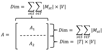
Proof. 

For ease of explanation, we denote $A$ as the coefficient matrix of variables $y_{stmv}$, which includes $A_1$ associating with constraints (2) and $A_2$ associating with constraints (3). The structure of $A$ can be presented as follows:

Firstly, according to [15], a sufficient condition for a matrix $M$ to be TU is: row indices of matrix $M$ can be partitioned into two sets such that the following four conditions are all satisfied: (i) each entry $m_{ij}$ of $M$ satisfies $m_{ij}\in \{\mathrm{0,1},-1\}$; (ii) each column of $M$ contains at most two non-zero entries; (iii) if a column has two entries of the same sign, their row indices are in different sets; and (iv) if a column has two entries of different signs, their row indices are in the same set.

For our matrix $A$, we consider dividing it naturally into two sets $A_1$ and $A_2$. For $A_1$ and $A_2$, each column contains only one 1, respectively. This implies that there are no more than two nonzero entries per column in the matrix $A$. Therefore, conditions (i)–(ii) are satisfied immediately. Then, we can partition all rows of $A_1$ into a set and that of $A_2$ into another, meeting the criteria (iii) and (iv). Thus, we conclude that matrix $A$ is TU. □

The primary benefit of this TU property lies in its ability to relax integer variables to continuous ones without changing the integer nature of the optimal solutions, thus reducing the computational time of the MIP model. Specifically, given any fixed integer variables $x_{tv},\forall t\in T, \forall v\in V,$ and integer parameters $b_v, \forall v\in V,$ the right-hand side of the constraints (3) are always integers. Considering that the coefficient matrix of $y_{stmv}$ is TU and the right-hand side of constraints (2) and (3) are integers, the binary variables $y_{stmv}$ can be relaxed to continuous variables.

3.3.3. Submodular Property of the Objective Function

For effective and cost-efficient decision-making in infrastructure planning, it is important to understand how the objective function behaves as more tank cleaning stations are built. Specifically, uncovering whether the model exhibits diminishing returns with additional facilities provides valuable guidance for resource allocation and investment decisions. To this end, we investigate the mathematical structure of the objective function to reveal any inherent properties that could impact strategic planning.

A set function $f:2^W\to \mathbb{R}$ defined on the subsets of a finite set $W$ is called submodular if it satisfies the diminishing returns property: for every $W_1\subseteq W_2\subseteq W$ and every $w\in W\setminus W_2$, it holds that $f(W_1\cup \{w\left\}\right)-f\left(W_1\right)\ge f(W_2\cup \{w\left\}\right)-f\left(W_2\right)$ [41]. In simple terms, a submodular function is a set function that describes the relationship between a set of inputs and an output, where adding more of one input has a decreasing additional benefit (diminishing returns). This property essentially means that the marginal gain from adding an element to a smaller set is at least as great as the gain from adding the same element to a larger set. Submodular functions are particularly interesting because they help model a variety of naturally occurring phenomena, such as economies of scale, network effects, or the spread of information in social networks.

For notation convenience, we denote $\mathit{x}={\left(x_{tv}\right)}_{t\in T, v\in V}$ and $\mathit{y}={\left(y_{stmv}\right)}_{ s\in S,t\in T, m\in M_{st},v\in V}$, which are restricted in the feasible region $\Omega$. Then, the objective function can be presented by a function of $\mathit{x}$ and $\mathit{y}$, denoted by $F_{\Omega }(\mathit{x},\mathit{y})$. We then give the following theorem about $F_{\Omega }(\mathit{x},\mathit{y})$.

Theorem 3.

The objective function $F_{\Omega }(\mathit{x},\mathit{y})$ is submodular regarding variables $\mathit{x}$.

Proof. 

Assuming that the annual budgets $B_t$and the construction capacity $K_v$ at each location $v$ are large enough, we can model our problem as a variant of the multi-dimensional set covering problem. Here, the objective is to minimize the cost of selecting a subset of locations $x_{tv}$ to cover all required service elements ${\sum }_{v\in V}{y}_{stmv}$. The set covering function is known to be submodular [41], which suggests that our objective function $F_{\Omega }(\mathit{x},\mathit{y})$ is also submodular with respect to the variables $\mathit{x}$.

In the subsequent contents, we prove this submodularity by a more rigorous step-by-step analysis.

Step 1: The integer variables $x_{tv}$ that indicates the number of tank cleaning stations constructed at location $v$ in the $t$-th year can be equivalently transformed intro binary variables ${\chi }_{tvk}$ that indicate whether the k-th tank cleaning station is constructed at location $v$ in the $t$-th year. Define ${\mathit{\chi }}_1$ and ${\mathit{\chi }}_2$ as two subsets of constructed tank cleaning stations and let ${\mathit{\chi }}_1\subseteq {\mathit{\chi }}_2\subseteq \mathit{\chi }$, where each ${\chi }_{tvk}\in \mathit{\chi },\forall t\in T,v\in V,k\in K_v,$ is 1. Then, for any ${\chi }_{t^{\prime }{v}^{\prime }{k}^{\prime }}\notin {\mathit{\chi }}_2$, the marginal gain by adding another tank cleaning station ${\chi }_{t^{\prime }{v}^{\prime }{k}^{\prime }}$ to ${\mathit{\chi }}_1$ can be defined as $F_{\Omega }\left({\mathit{\chi }}_1,\mathit{y}\right)-F_{\Omega }\left({\mathit{\chi }}_1\bigcup \left\{1\right\},\mathit{y}\right)$. We note that the marginal gain is represented by $F_{\Omega }\left({\mathit{\chi }}_1,\mathit{y}\right)-F_{\Omega }\left({\mathit{\chi }}_1\bigcup \left\{1\right\},\mathit{y}\right)$ since the objective function is the cost. Similarly, $F_{\Omega }\left({\mathit{\chi }}_2,\mathit{y}\right)-F_{\Omega }\left({\mathit{\chi }}_2\bigcup \left\{1\right\},\mathit{y}\right)$ is the marginal gain by adding the same tank cleaning station.

Step 2: Since ${\mathit{\chi }}_1\subseteq {\mathit{\chi }}_2$, any potential cost reduction in service coverage by adding ${\chi }_{t^{\prime }{v}^{\prime }{k}^{\prime }}$ to ${\mathit{\chi }}_2$ is also possible when added to ${\mathit{\chi }}_1$, but may remain unchanged due to already covered demands with the same cost. Therefore, the marginal gain is by adding another tank cleaning station ${\chi }_{t^{\prime }{v}^{\prime }{k}^{\prime }}$ to the existing subsets of stations ${\mathit{\chi }}_1$ is greater than or equal to adding it to ${\mathit{\chi }}_2$.

Step 3: If the annual budgets or construction capacities are not sufficient, the possibility of exceeding these constraints when adding ${\chi }_{t^{\prime }{v}^{\prime }{k}^{\prime }}$ to ${\mathit{\chi }}_2$ is higher than adding it to ${\mathit{\chi }}_1$, potentially yielding zero additional gain.

Conclusively, we always have $F_{\Omega }\left({\mathit{\chi }}_1,\mathit{y}\right)-F_{\Omega }\left({\mathit{\chi }}_1\bigcup \left\{1\right\},\mathit{y}\right){\ge F}_{\Omega }\left({\mathit{\chi }}_2,\mathit{y}\right)-F_{\Omega }\left({\mathit{\chi }}_2\bigcup \left\{1\right\},\mathit{y}\right)$, which completes the proof. □

4. Experiments

This section conducts computational experiments to verify the effectiveness of our proposed model. The experiments were conducted on a desktop computer equipped with 3.40 GHz of 13th Gen Intel Core i7 CPU and 32 GB of RAM, and the MIP model was solved by the Gurobi Optimizer 10.0.1 via the Python 3.11.5 API. We first set initial values for parameters to obtain basic results. Furthermore, sensitivity analyses are conducted to examine the impact of these parameters.

4.1. Experiment Settings

Taking the Yangtze River as an example, we select twenty-six ports ($\left|V\right|=26$) along the river as candidate locations where tank cleaning stations could be constructed. We focus on the river segment that starts from Chongqing, flows downstream through intermediate locations, and ends at Shanghai.

Table 3. The distance from Chongqing to downstream locations.

Port ID	Destination	Distance (km)	Port ID	Destination	Distance (km)	Port ID	Destination	Distance (km)
1	Chongqing	0	10	Hankou	1274	19	Ma’anshan	1959
2	Fuling	120	11	Yangluo	1306	20	Nanjing	2007
3	Wanxian	327	12	Huangshi	1417	21	Zhenjiang	2094
4	Badong	538	13	Wuxue	1493	22	Gaogang	2152
5	Yichang	648	14	Jiujiang	1543	23	Jiangyin	2211
6	Zhicheng	704	15	Anqing	1707	24	Zhangjiagang	2229
7	Shashi	796	16	Chizhou	1767	25	Nantong	2271
8	Chenglingji	1043	17	Tongling	1803	26	Shanghai	2399
9	Honghu	1095	18	Wuhu	1911

presents the distances from Chongqing to each port, with data sourced from J.H. Shipping Center [42]. Given that the river can be regarded as a line and the ports as points along this line, the distances between any two ports can be calculated based on Table 3. The map of the region under consideration is presented in Figure 2.

Table 4. Notations used in the experiment.

$\eta$	Annual growth rate of tank cleaning demand
$C_v^{\mathrm{b}\mathrm{a}\mathrm{s}\mathrm{e}}$	Baseline cost of constructing a candidate tank cleaning station at location $v$ in the first year of planing horizon
${\lambda }_t$	Inflation rate in the $t$-th year which affects the construction cost of tank cleaning stations
${\delta }_t$	The reduction rate of construction costs due to technological progress and labor cost decline in the $t$-th year
${\alpha }_v$	The ratio of the annual operating cost to the construction cost of tank cleaning stations at location $v$
$u_{\mathrm{s}\mathrm{t}\mathrm{a}\mathrm{n}}$	Standard speed of all ships
$u_{stmv}^D$	Sailing speed for ship $s$ visits the tank cleaning station at location $v$ after the $m$-th transportation task in the $t$-th year
${\tau }_{stmv}$	Time between the arrival of ship $s$ at the destination port of task $m$ and its arrival at the origin port of the next task in the $t$-th year, during which the ship visits a tank cleaning station at location $v$
${\gamma }_{st}$	Unit fuel price of ship $s$ in the $t$-th year
$U_{tv}$	The utilization rate of tank cleaning stations at location $v$ in the $t$-th year
$U_v$	The average annual utilization rate of tank cleaning stations at location $v$ in the planing horizon
$r$	The ratio of the actual sailing time of each cleaning task to its original sailing time at standard speed

summarizes the notations used in the experiment.

We categorize the parameters into the following three types:

• Capacity-Related Parameters. The planning period for this study is from 2025 to 2030, i.e., $\left|\mathrm{T}\right|=6$. The strategic placement of tank cleaning stations along the Yangtze River must adhere to the Yangtze River Waterway Tank Cleaning Station Layout Plan [17], which mandates proximity to chemical industrial clusters, shipyards, and hazardous cargo anchorages while maintaining distance from urban centers. Stations must also align with regional land use plans and possess integrated wastewater treatment infrastructure. For instance, ports like Nanjing and Yangluo (Wuhan) host large-scale chemical parks (e.g., Nanjing Chemical Industrial Park and Wuhan Chemical Industry Zone) and existing wastewater treatment facilities, satisfying both demand and regulatory thresholds. Conversely, ports adjacent to ecologically sensitive zones (e.g., Badong, Honghu) or dominated by non-hazardous cargo (e.g., Chizhou) are excluded due to environmental and operational incompatibility. Shanghai is prohibited from establishing tank cleaning stations due to its status as a densely populated urban core, which violates the distance from city centers mandate. Additionally, strict ecological red line restrictions, such as those in the Chongming Wetland Reserve, contribute to this prohibition. Based on the above criteria,

  Table 5. Maximum number of tank cleaning stations can be constructed at location $v$.

  Port Location	${\mathit{K}}_{\mathit{v}}$
  Nanjing, Yangluo, Nantong	3
  Chongqing, Fuling, Yichang, Zhicheng, Chenglingji, Jiujiang, Zhenjiang, Gaogang, Jiangyin	2
  Wanxian, Shashi, Hankou, Huangshi, Anqing, Tongling, Wuhu, Ma’anshan, Zhangjiagang	1
  Shanghai, Badong, Honghu, Wuxue, Chizhou	0

  categorizes the maximum allowable number of tank cleaning stations for each port, grouped by identical $K_v$ values.
• Demand-Related Parameters. According to [17], the annual tank cleaning demand growth rate is derived from a baseline demand of 8100 ship-times in 2025. The term “ship-times” refers to the total number of tank cleaning events for all ships within a given year. The annual tank cleaning demand $\eta$ is projected to increase at a compound annual growth rate (CAGR) of 5.0%. This projection is supported by recent data from the Yangtze River shipping sector, where the mainline port cargo throughput reached 4.02 billion tons in 2024, marking a 3.9% year-on-year increase, and the pilotage cargo volume rose by 6% over the same period [43]. These figures indicate a consistent upward trend in inland waterway freight transport, particularly in the Yangtze River region, which is a significant driver of demand for tank cleaning services. Therefore, a 5.0% CAGR for tank cleaning demand is a reasonable estimate, reflecting the overall growth in cargo volumes and the associated increase in cleaning requirements. Based on this growth rate, the annual tank cleaning demand is expected to reach 10,338 ship-times by 2030. The annual tank cleaning demand for each year is shown in

  Table 6. Projected annual tank cleaning demand from 2025 to 2030.

  Year	Projected Tank Cleaning Demand (Ship-Times)
  2025	8100
  2026	8505
  2027	8930
  2028	9377
  2029	9846
  2030	10,338

  . This linear extrapolation assumes synchronized growth between hazardous cargo volumes and cleaning demand. According to the baseline capacity for the initially planned stations as specified in [17], the parameter $b_v$ of the tank cleaning capacity of each candidate station is fixed at 600 ship-times per year.
• Cost-Related Parameters. For the parameter $C_{tv}$, the construction cost of a candidate tank cleaning station at location $v$ is calculated using a time-variant adjustment model, which is expressed as:

  $$C_{tv}=C_v^{\mathrm{b}\mathrm{a}\mathrm{s}\mathrm{e}}\cdot {\prod }_{\tau =2}^t\left(1+{\lambda }_{\tau }\right)\left(1-{\delta }_{\tau }\right),$$

  (10)

  where $C_v^{\mathrm{b}\mathrm{a}\mathrm{s}\mathrm{e}}$ represents 2025 baseline cost of constructing a candidate tank cleaning station at location $v$ derived from engineering bids (CNY 2.9 billion for upstream ports like Yichang [44], CNY 3.0 billion for midstream ports like Yueyang [45], and exceeding 2.0 billion CNY/station for downstream ports like Nanjing [46], with this study defining the baseline cost for downstream ports as CNY 2.5 billion). Upstream ports include Chongqing to Badong, midstream ports include Yichang to Jiujiang, and downstream ports include Anqing to Shanghai. The inflation rate ${\lambda }_t$ is set at 2.8% based on China’s Construction Price Index [47]. ${\delta }_t$ represents the annual decrease in construction costs due to technological advancements and reductions in labor costs. We set it at 5% per annum. For parameter $B_t$, we set $B_t=\mathrm{C}\mathrm{N}\mathrm{Y}20$ million ($\forall t\in T$).

The operating cost of a candidate tank cleaning station at location $v$ in the $t$-th year is modeled as a time-dependent function, calculated as:

$$O_{tv}=C_{tv}\cdot {\alpha }_v, \forall t\in T, \forall v\in V,$$

(11)

where ${\alpha }_v$ is a regional adjustment factor. For downstream ports where labor and energy costs are higher, ${\alpha }_v$ is set at 0.15. Conversely, upstream and midstream ports have a lower ${\alpha }_v$ of 0.10 due to more less stringent environmental enforcement and the advantage of lower labor costs. This factor allows for a more accurate representation of the operational costs in relation to the unique circumstances of each port’s location.

According to [17], as of the beginning of 2025, there have been 15 existing tank cleaning stations located at specific ports within the set of candidate locations considered in this study. The locations and the number of tank cleaning stations at each port are detailed in

Table 7. Existing tank cleaning stations in 2025.

Port Location	Number of Tank Cleaning Stations
Chongqing	2
Chenglingji	1
Yichang	1
Yangluo	1
Jiujiang	1
Anqing	1
Nanjing	3
Zhenjiang	1
Gaogang	1
Jiangyin	1
Nantong	2
Total	15

.

The construction costs of these pre-existing stations are not included in the model. However, their annual operating costs from 2025 to 2030 contribute to the total cost calculation. The model focuses on determining the optimal locations, timing, and number of new tank cleaning stations to be constructed from 2025 to 2030, building upon this existing infrastructure.

In this study, the Yangtze River’s cargo fleet is categorized into three classes based on tonnage: small ships with a tonnage of less than 1000 tons, medium ships with a tonnage ranging from 1000 to 3000 tons, and large ships with a tonnage exceeding 3000 tons. All three ship classes are powered by diesel engines. Referring to [48], the hourly consumption of ship $s$ sailing at speed $u$ is expressed as:

$$f_s\left(u\right)=C_{\mathrm{s}}^0+C_{\mathrm{s}}^1·u^{n_s},$$

(12)

where $n_s$ is the class-specific speed exponent, which is 3.5 for small ships, 4.0 for medium ships, and 4.5 for large ships. $C_{\mathrm{s}}^0$ and $C_{\mathrm{s}}^1$ are coefficients determined by the tonnage of ship $s$. Essentially, Equation (12) captures how a ship’s fuel consumption per hour increases more rapidly than its speed increases, due to the speed exponent $n_s$ being considerably larger than 1. This highlights the substantial fuel consumption when ships must travel faster to finish transportation tasks on time. In the fleet under consideration, small ships account for 30%, medium ships account for 40%, and large ships account for 30%.

Table 8. Fuel consumption of different ship classes.

Ship Class	${\mathit{C}}_{\mathit{s}}^0$	${\mathit{C}}_{\mathit{s}}^1$	${\mathit{n}}_{\mathit{s}}$	Standard Speed (km/h)	Standard Fuel Consumption (kg/h)
Small	598.65	0.0198	3.5	16	923.1
Medium	649.65	0.0040	4.0	16	911.8
Large	600.45	0.0009	4.5	16	836.4

illustrates the parameter values for three classes of ships, with $C_s^0$ and $C_s^1$ coefficients derived from the median of the value ranges provided in [48]. The table specifies the types of fuel used by each ship class and their standard operating speeds. Additionally, it provides the calculated fuel consumption rates for each ship type during standard speed operation.

In the planning horizon, for all transportation tasks of all ships, the sailing speed required for a ship to complete a task on time without taking a detour is set as the standard speed $u_{\mathrm{s}\mathrm{t}\mathrm{a}\mathrm{n}}$. However, if the ship takes a detour to the cleaning station at location $v$, it must increase its speed to $u_{stmv}^D$ to maintain the schedule. The relationship between the standard speed $u_{\mathrm{s}\mathrm{t}\mathrm{a}\mathrm{n}}$ and the detour speed $u_{stmv}^D$ is constrained by the time invariance condition, where the sailing time ${\tau }_{stmv}$ remains unchanged. This condition is expressed as ${\tau }_{stmv}=d_{v_{stm}^{\mathrm{d}\mathrm{e}\mathrm{s}\mathrm{t}}{v}_{st\left(m+1\right)}^{\mathrm{o}\mathrm{r}\mathrm{i}\mathrm{g}}}/u_{\mathrm{s}\mathrm{t}\mathrm{a}\mathrm{n}}=\left(d_{v_{stm}^{\mathrm{d}\mathrm{e}\mathrm{s}\mathrm{t}}v}+d_{v{v}_{st\left(m+1\right)}^{\mathrm{o}\mathrm{r}\mathrm{i}\mathrm{g}}}\right)/u_{stmv}^D$, which yields $u_{stmv}^D=u_{\mathrm{s}\mathrm{t}\mathrm{a}\mathrm{n}}·\left(d_{v_{stm}^{\mathrm{d}\mathrm{e}\mathrm{s}\mathrm{t}}v}+d_{v{v}_{st\left(m+1\right)}^{\mathrm{o}\mathrm{r}\mathrm{i}\mathrm{g}}}\right)/d_{v_{stm}^{\mathrm{d}\mathrm{e}\mathrm{s}\mathrm{t}}{v}_{st\left(m+1\right)}^{\mathrm{o}\mathrm{r}\mathrm{i}\mathrm{g}}}$. Thus, the additional fuel consumption $F_{stmv}$ accounts for the detour taken by ship $s$ when it visits the tank cleaning station at location $v$ after the $m$-th transportation task in the $t$-th year. This additional fuel consumption can be expressed as $F_{stmv}=\left(f_s\left(u_{stmv}^D\right)-f_s\left(u_{\mathrm{s}\mathrm{t}\mathrm{a}\mathrm{n}}\right)\right)·{\tau }_{stmv}$. The detour cost $C_{stmv}^D$ can then be calculated as the product of the fuel price and the additional fuel consumption, i.e., $C_{stmv}^D={\gamma }_{st}·F_{stmv}^D$. Under the net-zero emissions scenario, crude oil demand is projected to decline between 2025 and 2030, with an average annual price decrease of 2.5% [49]. Therefore, we assume that fuel price, with a 2025 base price of CNY 8.0/kg, decreases by 2.5% annually.

After establishing the parameter settings, we used these values to derive the basic results, and then we conducted a sensitivity analysis to examine the impacts of these parameters.

4.2. Basic Results

This section gives a detailed analysis of the basic results derived from the MIP model. The analysis focuses on evaluating the construction strategy of new tank cleaning stations, assessing the utilization rate of tank cleaning stations at each port, and examining the rationality of detour distances and detour speeds under the optimal layout of tank cleaning stations. The analysis is essential for evaluating the model’s performance.

4.2.1. Tank Cleaning Station Construction Strategy

In this section, we present the results of the MIP model solved by Gurobi. The results related to the construction strategy are presented in

Table 9. Results related to the construction strategy.

Year	Port Location of New Tank Cleaning Station	Number of Stations Constructed	Construction Cost (CNY Million)	Remaining Budget (CNY Million)
2025	Wuhu	1	250.0	0
2026	Tongling	1	244.2	5.8
2027	NA	0	0	255.8
2028	Wanxian	1	270.1	235.7
2029	NA	0	0	485.7
2030	NA	0	0	735.7

.

The results indicate a phased construction approach in the planning horizon, with a focus on the initial years. Specifically, the model recommends constructing a single station at Wuhu in 2025, incurring a cost of 250 million CNY and fully utilizing the allocated budget for that year. In 2026, a station is constructed at Tongling, costing CNY 244.2 million, leaving a small remaining budget of CNY 5.8 million. No construction is scheduled for 2027, during which the remaining budget accumulates. In 2028, a station is constructed at Wanxian, costing CNY 270.1 million. No additional tank cleaning stations are planned for 2029 and 2030, as the increased costs of constructing new stations would exceed the benefits from reduced detour costs, thereby increasing the objective function value.

4.2.2. Utilization Rate of Tank Cleaning Stations at Each Port

To evaluate the efficiency of the tank cleaning station construction strategy and prevent either under-utilization or over-utilization scenarios, we conduct an analysis of the annual average utilization rate of tank cleaning stations at each port. The actual number of cleaning services provided by all tank cleaning stations at port $v$ in the $t$-th year is denoted as $Q_{tv}^{\mathrm{t}\mathrm{o}\mathrm{t}\mathrm{a}\mathrm{l}}$, while the total annual cleaning capacity of all stations at the same port $v$ in a year is represented by $b_v^{\mathrm{t}\mathrm{o}\mathrm{t}\mathrm{a}\mathrm{l}}$. The utilization rate of tank cleaning stations at port $v$ in the $t$-th year $U_{tv}$ is calculated as $U_{tv}=Q_{tv}^{\mathrm{t}\mathrm{o}\mathrm{t}\mathrm{a}\mathrm{l}}/b_v^{\mathrm{t}\mathrm{o}\mathrm{t}\mathrm{a}\mathrm{l}}$. The average annual utilization rate $U_v$ in the planning horizon is computed as the arithmetic mean of the annual utilization rates, i.e., $U_v={\displaystyle \frac{1}{T}}{\sum }_{t=1}^T{U}_{tv}$.

A high utilization rate, especially when approaching 100%, can result in multiple issues. These include longer waiting times for ships, inefficiencies in the cleaning process, and increased wear and tear on equipment. By analyzing the annual average utilization rate of tank cleaning stations at each port, we can assess the balance of the current tank cleaning station construction plan in terms of resource allocation across different ports.

Table 10. Annual average utilization rate of tank cleaning stations at each port.

Port Location	${\mathit{U}}_{\mathit{v}}$	Construction Year
Chongqing	88.7%	Existing
Wanxian	92.7%	2028
Yichang	94.5%	Existing
Chenglingji	95.6%	Existing
Yangluo	92.5%	Existing
Jiujiang	91.3%	Existing
Anqing	96.1%	Existing
Tongling	93.8%	2025
Wuhu	80.3%	2026
Nanjing	89.4%	Existing
Zhenjiang	84.5%	Existing
Gaogang	83.6%	Existing
Jiangyin	86.5%	Existing
Nantong	77.5%	Existing
Avg	89.1%

presents the annual average utilization rate of tank cleaning stations at each port. The third column of the table indicates the construction year of the tank cleaning stations at each port. For ports where this column is marked as “Existing”, the tank cleaning stations were already in operation before the planning period began.

The results indicate that the annual average utilization rates of tank cleaning stations vary among different ports. For ports with high utilization rates, such as Yichang (94.5%), Chenglingji (95.6%), and Anqing (96.1%), although the utilization rates are relatively high, they do not approach 100% closely. In contrast, ports with relatively lower utilization rates, such as Nantong (77.5%), still maintain utilization rates above 75%, which indicates the resources in these ports are not being wasted excessively. The relatively lower utilization rate in Nantong can be attributed to the fact that two tank cleaning stations were already in operation before the planning period began in 2025. As a result, during the initial years of the planning horizon, the number of cleaning services provided by these stations was relatively low compared to their total cleaning capacity. This led to a lower overall utilization rate for the port in the planning period.

With an average annual utilization rate of 89.1% across all ports, the tank cleaning stations are generally operating efficiently.

4.2.3. Ship Detour Analysis

Based on the optimal layout of tank cleaning stations derived from the MIP model, an analysis is conducted on the detour distances, differences between detour speeds and standard speeds, the detour costs, and the ratios of these detour costs to the total system costs for all transportation tasks of each ship in the planning horizon. The detour speed is crucial as it reflects the actual sailing speed of the ship when it has to deviate from its normal route. Additionally, the detour costs and their proportion relative to the total costs provide insights into the economic impact of these detours.

Table 11. Details of the top 5 transportation tasks with the longest detours.

Transportation Task ID	Detour Distance (km)	Detour Speed (km/h)	Percentage Difference Between Detour Speed and Standard Speed	Detour Cost (CNY 10,000)
1	240	34.6	116.3%	46.3
2	220	32.7	104.4%	23.0
3	112	35.5	121.9%	22.7
4	100	37.0	131.3%	22.1
5	64	21.7	35.6%	5.6

presents the details of the top five transportation tasks with the longest detours among all tasks performed by all ships in the planning horizon. For each of these tasks, the table shows the detour distance, the detour speed, the percentage difference between the detour speed and the standard speed, and the detour cost. This helps in analyzing whether the detour distances and detour speeds of ships are within reasonable limits under the optimal solution of the MIP model, preventing excessively long detours and unreasonably high actual sailing speeds that deviate from realistic conditions. Additionally, examining the ratios of detour costs to the total costs allows us to assess the financial impact of detours.

The results indicate that there is a wide spectrum of detour distances, with Task 1 having the maximum detour at 240 km and Task 5 at 64 km. This variation in detour distances directly influences other aspects, such as detour speed and cost. The detour speeds range from 21.7 km/h (Task 5) to 37.0 km/h (Task 4), and the percentage differences between detour speeds and standard speeds also differ notably. For instance, Task 4 has a 131.3% difference, suggesting that in certain tasks, the detour speed is much higher than the standard speed. However, all detour speeds in the table, including that of Task 4, remain within a reasonable range, validating the reliability of the model’s results. The detour costs, measured in CNY 10,000, vary from 5.6 (Task 5) to 46.3 (Task 1), clearly showing the financial implications of these detours. Additionally, the overall proportion of detour trips is only 1.01% of all trips in the planning period, demonstrating that the vast majority of trips do not require a detour. Furthermore, the average detour distance across all trips is just 1.42 km, further reinforcing the effectiveness of the model in minimizing unnecessary detours. These results highlight the model’s success in optimizing routing decisions and reducing the overall detour burden while maintaining reasonable operational efficiency.

Based on the MIP model’s calculations, the total construction cost is CNY 0.77 billion, the total operation cost is CNY 3.24 billion, and the total detour cost is CNY 0.22 billion. These values sum up to a total cost of CNY 4.23 billion. Notably, the detour cost accounts for only 5.2% of the total cost, which indicates that the proportion of detour cost is relatively small and implies that the new construction of tank cleaning stations can ensure that ships have relatively short detour distances in the planning horizon.

4.2.4. Key Insights and Model Effectiveness

Based on the above analysis of the main results, the key insights are summarized as follows:

• The model recommends a phased construction strategy, concentrating new station construction in the early years of the planning horizon to effectively utilize the annual budget. It also defers additional construction when marginal returns diminish. The phased investment approach and optimized routing under the model achieve both high operational efficiency and cost-effectiveness across the network.
• Average annual utilization rates of tank cleaning stations are high (averaging 89.1%), with utilization consistently above 75% even at lower-demand ports, indicating efficient resource allocation and minimal capacity waste.
• Variation in detour distances, speeds, and costs among different tasks is observed; however, all detour speeds remain reasonable, and detour trips constitute only 1.01% of total trips, with an average detour distance of just 1.42 km, validating the model’s effectiveness in minimizing unnecessary detours.
• The majority of overall cost is attributed to operation and construction, with detour costs accounting for only 5.2%, demonstrating that optimized station deployment successfully limits the economic impact of detours.

4.3. Sensitivity Analysis

By conducting sensitivity analysis experiments, we further analyze the sensitivity of the methods to the changes in input parameters, including the annual budget, the capacity of each candidate tank cleaning station, and the actual sailing time of each transportation task.

The parameters of the experiments are set as shown in

Table 12. Experiment parameter settings.

GID	EID	${\mathit{B}}_{\mathit{t}}$ (CNY Million)	${\mathit{b}}_{\mathit{v}}$	$\mathit{r}$	$\mathbf{MT}$
G0	0–7	[150, 500, 50]	600	1	MIP
G1	8–14	250	[300, 900, 100]	1	MIP
G2	15–21	250	600	[0.7, 1.3, 0.1]	MIP
G3	22–29	[150, 500, 50]	600	1	PRMIP
G4	30–36	250	[300, 900, 100]	1	PRMIP
G5	37–43	250	600	[0.7, 1.3, 0.1]	PRMIP

. Generally, we conduct 44 experiments with experiment ID (EID) indexed from 0 to 43. Each of the experiments is included in the corresponding group with a group ID (GID). G0, G1, and G2 are the groups of experiments that aim to illustrate the performance of the MIP model in solving instances with different annual budget ($B_t$), the capacity of each candidate tank cleaning station ($b_v$), and the ratio of the actual sailing time of each task to its original sailing time, respectively. The ratio is denoted as $r$, where the original sailing time is ${\tau }_{stmv}$, the actual sailing time is ${\tau }_{stmv}^{\mathrm{a}\mathrm{c}\mathrm{t}\mathrm{u}}$, and $r={\tau }_{stmv}^{\mathrm{a}\mathrm{c}\mathrm{t}\mathrm{u}}/{\tau }_{stmv}$. Accordingly, the results of G3, G4, and G5 are generated by a PRMIP model. “MT” represents the model type, including the MIP model and the PRMIP model. In the “$B_t$ (CNY million)”, “$b_v$”, and “$r$” columns, $[a, b, c]$ represents a list of numbers generated from $a$ to $b$ with a step size of $c$.

4.3.1. Different Annual Budget

To investigate the impact of varying the annual budget on the model’s effectiveness, we design instances by altering the annual budget from 150 million to 500 million while keeping the capacity of each candidate tank cleaning station ($b_v=600$) and the sailing time ratio ($r=1$) unchanged.

Figure 3 and Figure 4 show the optimal results of the MIP model and the PRMIP model, respectively. The x-axis represents the EID, where instances are arranged in increasing order of the annual budget. The y-axis corresponds to the values of indicators, including the objective of an optimal solution (Obj), the total number of tank cleaning stations constructed (TCSN) and the total construction cost (TCSC) in the planning horizon, the average utilization rate (AUR) of all tank cleaning stations in the planning horizon, and the average detour distance (ADD) of all ships along with the average percentage difference between detour speeds and standard speeds (PDS) in the planning period.

As shown in Figure 3 and Figure 4, increasing the annual budget from CNY 150 to 300 million leads to a significant decline in total cost before plateauing. This reduction is primarily driven by a noticeable decrease in detour costs, which result from reductions in ADD and PDS. Both the MIP and PRMIP models show similar trends across all key metrics, indicating that relaxing ship assignment variables does not significantly affect the overall results.

A higher annual budget relaxes budget constraints, allowing for more flexibility in construction planning. This enables the earlier construction of tank cleaning stations or the establishment of multiple stations, which increases the total available cleaning capacity over the planning period. As a result, the AUR decreases, as the stations provide cleaning services for a longer duration. Additionally, TCSC rises slightly due to earlier construction in higher-budget scenarios, which is attributed to the cost parameter settings in Equation (10), where the construction cost of tank cleaning stations at a port decreases over the planning period. Optimizing the construction timing and location of new tank cleaning stations allows ships to access cleaning stations with shorter detours, further reducing ADD and PDS and improving overall operational efficiency.

Notably, TCSN remains constant at three across all budget levels. This suggests that constructing the first three stations yields a significant reduction in detour costs, outweighing the additional construction and operational costs. However, attempting to build a fourth station would lead to diminishing returns, where the reduction in detour costs would no longer offset the additional construction and operational costs. This phenomenon aligns with Theorem 3, which states that the objective function is submodular concerning the constructed station number. The submodular property implies that the marginal benefit of adding a station decreases as more stations are introduced. In this case, the first few stations contribute significantly to reducing detour costs, but beyond a certain point, additional stations would not provide more benefits.

Overall, increasing the annual budget enhances operational efficiency and reduces detour costs. However, the choice between MIP and PRMIP does not substantially impact the key performance indicators.

Table 13. Optimal results of the MIP model with different annual budgets (EID: 0–7).

EID	${\mathit{B}}_{\mathit{t}}$ (CNY Million)	Obj (CNY Million)	TCSN	TCSC (CNY Million)	AUR (%)	ADD (km)	PDS (%)	CPU Time (s)
0–7	150	4320.7	3	741.7	90.6	2.29	2.0	262.8
	200	4304.0	3	753.6	89.6	1.80	1.6	173.7
	250	4237.7	3	759.4	89.1	1.42	1.2	312.4
	300	4229.5	3	771.7	87.5	0.92	0.9	212.2
	350	4229.5	3	771.7	87.5	0.92	0.9	266.2
	400	4229.5	3	771.7	87.4	0.92	0.9	269.0
	450	4229.5	3	771.7	87.6	0.92	0.9	243.7
	500	4229.5	3	771.7	87.6	0.92	0.9	233.9
Avg	325	4251.2	3	764.2	88.4	1.26	1.2	246.7

and

Table 14. Optimal results of the PRMIP model with different annual budgets (EID: 22–29).

EID	${\mathit{B}}_{\mathit{t}}$ (CNY Million)	Obj (CNY Million)	TCSN	TCSC (CNY Million)	AUR (%)	ADD (km)	PDS (%)	CPU Time (s)
22–29	150	4320.7	3	741.7	90.7	2.34	2.0	127.8
	200	4304.0	3	753.6	89.5	1.82	1.7	123.3
	250	4237.7	3	759.4	89.1	1.43	1.3	59.5
	300	4229.5	3	771.7	87.4	0.92	0.9	112.5
	350	4229.5	3	771.7	87.3	0.92	0.9	82.6
	400	4229.5	3	771.7	87.4	0.92	0.9	58.9
	450	4229.5	3	771.7	87.5	0.92	0.9	59.0
	500	4229.5	3	771.7	87.5	0.92	0.9	61.3
Avg	325	4251.2	3	764.2	88.3	1.27	1.2	85.6

display the outcomes of these analyses.

The MIP and PRMIP models produce the same optimized station layout, as Obj, TCSN, and TCSC are identical across all budget levels. While AUR, ADD, and PDS are not entirely the same, their average values are highly similar. This slight variation results from minor differences in ship routing. A notable difference between the two models is their computational efficiency. These findings suggest that while both MIP and PRMIP produce optimal solutions to the original problem, they may lead to different outcomes on some indicators due to the existence of multiple optimal solutions. The average CPU Time for the MIP model is 246.7 s, whereas the PRMIP model, with relaxed binary variables, significantly reduces computation time to an average of 85.6 s. In summary, the PRMIP model is significantly more computationally efficient than the MIP model without surrendering the solution quality, which aligns with Theorem 2.

Based on the above analysis of how the annual budget affects model outcomes, we summarize some key insights as follows:

• Increasing the annual budget substantially reduces total cost up to a threshold, after which cost savings plateau. This reduction is primarily due to decreased detour costs, enabled by more timely and flexible construction of cleaning stations, which improves overall system efficiency (as indicated by lower ADD and PDS).
• The number of constructed stations (TCSN) stabilizes at three, confirming that additional stations beyond this number provide diminishing returns, in line with the submodular nature of the objective function.
• Earlier and more frequent construction marginally increases total construction cost (TCSC), as station costs decline over the planning horizon.
• The choice between MIP and PRMIP models does not noticeably affect key performance metrics.
• Decision-makers can improve system efficiency by increasing the budget up to an optimal point, but excessive budget increases may not yield further benefits.

4.3.2. Different Station Capacity

To investigate the impact of varying the capacity of each candidate tank cleaning station on the model’s effectiveness, we design instances by altering the station capacity from 300 ship-times to 900 ship-times while keeping the annual budget ($B_t=250$) and the sailing time ratio ($r=1$) unchanged.

Figure 5 and Figure 6 show the optimal results of the MIP model and the PRMIP model, respectively.

As shown in Figure 5 and Figure 6, increasing station capacity leads to a decline in Obj, primarily due to reduced detour costs. This section examines the impact of capacity on key performance metrics.

Capacity significantly influences TCSN and TCSC. When capacity is low, more stations are required to meet demand, whereas higher capacities reduce TCSN. Initially, adding stations substantially reduces detour costs, but beyond a certain capacity, additional stations provide limited benefit.

AUR fluctuates due to two opposing effects. On the one hand, increasing capacity allows each station to serve more ships, reducing AUR. On the other hand, the concurrent decline in TCSN leads to higher utilization at the remaining stations, increasing AUR. As a result, AUR exhibits relatively large fluctuations across different capacity levels.

Trends in ADD and PDS show that when capacity is low, higher TCSN helps reduce detour costs, but limited station capacity can still force longer detours. As capacity increases, ADD and PDS initially decline due to better station accessibility. However, as TCSN declines significantly, fewer available stations force some ships to travel longer distances, leading to an increase in ADD and PDS. As a result, ADD and PDS exhibit relatively large fluctuations.

Overall, the model optimally balances the number and location of stations to minimize total costs, including construction, operation, and detour-related expenses. The fluctuations in AUR, ADD, and PDS highlight these complex trade-offs. Notably, MIP and PRMIP yield nearly identical results across key metrics, with PRMIP offering superior computational efficiency, as previously discussed.

Table 15. Optimal results of the MIP model with different station capacities (EID: 8–14).

EID	${\mathit{b}}_{\mathit{v}}$	Obj (CNY Million)	TCSN	TCSC (CNY Million)	AUR (%)	ADD (km)	PDS (%)	CPU Time (s)
8–14	300	4748.5	5	1203.6	91.0	2.24	2.0	206.3
	400	4493.1	4	981.5	88.6	1.42	1.2	181.4
	500	4244.8	3	758.6	89.8	1.78	1.6	196.7
	600	4237.7	3	759.4	89.1	1.42	1.2	218.7
	700	4107.5	2	526.6	90.1	3.32	3.5	313.7
	800	4042.6	2	494.2	88.4	3.16	3.3	234.8
	900	4032.5	2	482.9	87.1	3.01	3.2	183.4
Avg	600	4272.4	3	743.8	89.2	2.34	2.3	219.3

and

Table 16. Optimal results of the PRMIP model with different station capacities (EID: 30–36).

EID	${\mathit{b}}_{\mathit{v}}$	Obj (CNY Million)	TCSN	TCSC (CNY Million)	AUR (%)	ADD (km)	PDS (%)	CPU Time (s)
30–36	300	4748.5	5	1203.6	91.2	2.26	2.0	71.6
	400	4493.1	4	981.5	89.0	1.42	1.2	81.6
	500	4244.8	3	758.6	89.6	1.77	1.5	78.3
	600	4237.7	3	759.4	89.2	1.44	1.2	81.3
	700	4107.5	2	526.6	89.9	3.35	3.5	81.7
	800	4042.6	2	494.2	88.2	3.12	3.3	81.9
	900	4032.5	2	482.9	87.3	2.98	3.1	78.9
Avg	600	4272.4	3	743.8	89.2	2.33	2.3	79.3

display the outcomes of these analyses.

Table 15 and Table 16 present the numerical results for the MIP and PRMIP models under varying station capacities, revealing identical trends in Obj, TCSN, and TCSC. Minor differences in AUR, ADD, and PDS stem from variations in ship routing within multiple optimal solutions, consistent with previous findings. Notably, PRMIP maintains solution quality while achieving significantly higher computational efficiency than MIP.

Based on the above analysis of how station capacity affects model outcomes, we summarize some key insights as follows:

• Increasing station capacity generally reduces the objective value by lowering detour costs and requiring fewer total stations.
• When capacity is low, more stations are needed; as capacity increases, the optimal number of stations (TCSN) decreases, highlighting economies of scale.
• Average utilization ratio (AUR) and detour metrics (ADD, PDS) show noticeable fluctuations across different capacity levels, due to the interplay between station coverage and accessibility.
• The model effectively balances between station number, location, and capacity to minimize total system cost, capturing the trade-offs among construction, operation, and detour expenses.
• MIP and PRMIP models again yield essentially the same operational outcomes, but PRMIP demonstrates higher computational efficiency.

4.3.3. Different Sailing Time Ratio

To investigate the impact of varying the sailing time of each task on the model’s effectiveness, we design instances by altering sailing time ratio from 0.7 to 1.3 with a step size of 0.1, while keeping the annual budget ($B_t=250$) and the station capacity ($b_v=600$) unchanged.

Figure 7 and Figure 8 show the optimal results of the MIP model and the PRMIP model, respectively.

As shown in Figure 7 and Figure 8, which present the MIP and PRMIP model results under varying sailing time ratios, several key trends emerge. An increase in the sailing time ratio consistently leads to a decline in Obj, primarily due to reduced detour costs. Since sailing time is inversely related to speed, a longer sailing time corresponds to a lower travel speed, reducing the required speed adjustments for detours. This mitigates the exponential increase in fuel consumption associated with higher speeds, leading to lower detour costs and, consequently, a reduction in Obj.

TCSN and TCSC remain relatively stable across different sailing time ratios. TCSN is consistently three across all tested cases, indicating that the optimal number of stations is determined by cleaning demand and station capacity rather than sailing time. Minor fluctuations in TCSC arise due to construction timing decisions influenced by the cost parameters in Equation (10), rather than any direct dependence on the sailing time ratio. Similarly, AUR remains relatively stable, fluctuating around a central value, indicating that station utilization is not significantly affected by changes in sailing time.

ADD generally increases as the sailing time ratio increases, though with some fluctuations. This pattern is attributed to the exponential relationship between fuel consumption and speed, as defined in Equation (12). With high exponents (3.5, 4.0, and 4.5 for the different ship classes in this study), even small increases in speed lead to disproportionately large increases in fuel consumption and detour costs. At lower sailing time ratios (i.e., higher speeds), the model prioritizes shorter detours to limit excessive fuel consumption caused by speed adjustments. However, as the sailing time ratio increases, the cost of additional detours diminishes as lower speeds result in a smaller increase in fuel consumption. Consequently, the model allows for longer detours when they help offset construction and operational expenses. As a result, ADD exhibits an overall increasing trend with local fluctuations, reflecting the trade-off between construction costs, operational costs, and detour costs.

Table 17. Optimal results of the MIP model with different sailing time ratios (EID: 15–21).

EID	$\mathit{r}$	Obj (CNY Million)	TCSN	TCSC (CNY Million)	AUR (%)	ADD (km)	PDS (%)	CPU Time (s)
15–21	0.7	4659.4	3	759.4	89.6	1.44	43.1	218.2
	0.8	4466.0	3	764.3	88.3	1.74	25.2	295.2
	0.9	4338.3	3	759.4	89.2	1.42	11.3	215.7
	1.0	4237.7	3	759.4	89.1	1.42	1.2	303.5
	1.1	4163.8	3	747.5	89.9	1.91	8.9	244.5
	1.2	4086.4	3	699.5	92.0	3.30	16.4	198.1
	1.3	4025.0	3	699.5	92.2	3.30	22.8	161.8
Avg	1.0	4282.4	3	741.3	90.0	2.08	18.3	233.9

and

Table 18. Optimal results of the PRMIP model with different sailing time ratios (EID: 37–43).

EID	$\mathit{r}$	Obj (CNY Million)	TCSN	TCSC (CNY Million)	AUR (%)	ADD (km)	PDS (%)	CPU Time (s)
37–43	0.7	4659.4	3	759.4	89.3	1.44	43.1	78.2
	0.8	4466.0	3	764.3	88.2	1.74	25.2	70.5
	0.9	4338.3	3	759.4	88.7	1.46	11.4	73.7
	1.0	4237.7	3	759.4	88.9	1.42	1.2	86.2
	1.1	4163.8	3	747.5	90.1	1.91	8.9	70.3
	1.2	4086.4	3	699.5	92.7	3.30	16.4	77.7
	1.3	4025.0	3	699.5	92.2	3.30	22.8	58.5
Avg	1.0	4282.4	3	741.3	90.0	2.08	18.3	73.6

show results for MIP and PRMIP under varying sailing time ratios. Both models have identical trends in Obj, TCSN, and TCSC, confirming consistent station layouts. Minor variations in AUR, ADD, and PDS reflect differences in ship routing across optimal solutions. PRMIP achieves the same optimal solutions as MIP with better computational efficiency, evidenced by lower CPU time.

Based on the above analysis of how station capacity affects model outcomes, we summarize some key insights as follows:

• A higher sailing time ratio (lower speeds) leads to reduced total cost by mitigating the exponential effect of speed on fuel consumption, thereby lowering detour costs.
• The number of stations (TCSN) and total construction cost (TCSC) remain largely stable, indicating these are governed more by demand and capacity than by sailing time.
• Station utilization (AUR) is relatively insensitive to changes in the sailing time ratio.
• Average detour distance (ADD) tends to increase with the sailing time ratio due to relaxed constraints on speed-driven detour cost, but with local fluctuations reflecting the model’s trade-off decisions.
• Results suggest that adjusting sailing speed can be a useful lever to manage system costs, mainly through its impact on detour-related expenses rather than infrastructure needs.

To sum up, the numerical experiments, encompassing variations in annual budget, station capacity, and sailing time ratio (as detailed in Table 13, Table 14, Table 15, Table 16, Table 17 and Table 18), demonstrate that the MIP and PRMIP models consistently produce equivalent optimal solutions for tank cleaning station placement, validating Theorem 2. However, the PRMIP model achieves this with significantly greater computational efficiency. The sensitivity analyses reveal how changes in key input parameters, namely annual budget, station capacity, and sailing time ratio, influence the optimal solutions and key performance indicators, such as total cost, the number and location of stations, average utilization rates, and detour distances. Furthermore, the analysis highlights the importance of considering the submodular nature of the problem (Theorem 3) and the exponential relationship between fuel consumption and speed when making strategic decisions about tank cleaning station construction.

5. Conclusions

Inland waterway transportation is vital for the movement of hazardous liquid cargoes, but it faces significant operational challenges, particularly when tank cleaning is required between shipments to prevent contamination. This necessitates detours, which increase fuel consumption and operational costs, ultimately reducing system efficiency. Optimizing the placement of tank cleaning stations and assigning cleaning tasks are essential to minimize these costs.

To address this challenge, we propose an MIP model for the TCSL-CTA problem. The key findings and contributions of this study are summarized as follows:

• We develop a PRMIP model for the TCSL-CTA problem, supported by a series of theoretical results. In particular, we identify critical properties, such as the total unimodularity of the assignment constraint matrix and the submodularity of the objective function, which enable both stronger computational efficiency and practical insights for flexible and incremental facility planning.
• Through comprehensive case studies on the Yangtze River (2025–2030), we demonstrate that our approach efficiently produces feasible construction plans, with total costs, station utilization rates, and detour costs all quantitatively evaluated. Sensitivity analyses further illustrate how key parameters (e.g., budget, station capacity, sailing time ratios) influence plan effectiveness and resource allocation, delivering valuable managerial guidance for balancing construction station, construction timing, and detour cost.

Drawing from the limitations of the current study, two promising directions are identified for future work:

(1)

Developing robust optimization frameworks. Future research could develop robust optimization models to explicitly account for real-world uncertainties such as temporary port closures, equipment failures, or facility inaccessibility in tank cleaning station location and task allocation. These disruptions may render certain planned facilities unusable, resulting in costly recourse actions. Incorporating such risks is therefore essential for enhancing the practical resilience of the planning model. Prior studies have applied robust optimization techniques to similar facility location problems under disruption risk [50], which can serve as a methodological foundation for this extension.

(2)

Extending the model with real-time and adaptive decision-making. The current model can be enhanced by incorporating real-time decision-making capabilities through frameworks such as dynamic programming or reinforcement learning. These methods are well-suited for handling uncertainties in task arrivals, demand fluctuations, and facility availability. In particular, promising directions include multi-agent reinforcement learning for dynamic scheduling [51], condition-based risk management [52], AI-based autonomous task planning [53], and improved actor–critic algorithms [54]. These methodologies offer valuable insights for extending the current model to support dynamic programming-based solutions and online decision-making, particularly in scenarios characterized by randomly arriving tasks and frequent operational changes.