Estimation of Missing DICOM Windowing Parameters in High-Dynamic-Range Radiographs Using Deep Learning

Abstract

Digital Imaging and Communication in Medicine (DICOM) is a standard format for storing medical images, which are typically represented in higher bit depths (10–16 bits), enabling detailed representation but exceeding the display capabilities of standard displays and human visual perception. To address this, DICOM images are often accompanied by windowing parameters, analogous to tone mapping in High-Dynamic-Range image processing, which compress the intensity range to enhance diagnostically relevant regions. This study evaluates traditional histogram-based methods and explores the potential of deep learning for predicting window parameters in radiographs where such information is missing. A range of architectures, including MobileNetV3Small, VGG16, ResNet50, and ViT-B/16, were trained on high-bit-depth computed radiography images using various combinations of loss functions, including structural similarity (SSIM), perceptual loss (LPIPS), and an edge preservation loss. Models were evaluated based on multiple criteria, including pixel entropy preservation, Hellinger distance of pixel value distributions, and peak-signal-to-noise ratio after 8-bit conversion. The tested approaches were further validated on the publicly available GRAZPEDWRI-DX dataset. Although histogram-based methods showed satisfactory performance, especially scaling through identifying the peaks in the pixel value histogram, deep learning-based methods were better at selectively preserving clinically relevant image areas while removing background noise.

1. Introduction

Digital Imaging and Communication in Medicine (DICOM) serves as a standardized format for storing medical images along with their corresponding metadata, which are located in the file header [1]. It supports images obtained by different imaging techniques and can feature a range of bit depths, typically 10 to 16 bits [2], corresponding to thousands (even tens-of-thousands) of shades of gray. However, the majority of general-purpose monitors can show only 8 bits of image depth, meaning that there is an inevitable loss of information while viewing medical images on such displays [3]. More importantly, the human visual system has inherent limitations and can discriminate only between approximately 700 to 900 shades of gray, even under optimal viewing conditions [3].

At the same time, the rise of accessible computational power and the ever-increasing volume of available medical data [4] led to a rapid development of different systems based on machine learning (ML), which are designed to assist physicians during the diagnostic process [5]. These computer-aided diagnosis (CAD) systems can process various inputs, including medical images, to detect a variety of health conditions ranging from brain tumors [6] and liver diseases [7] to COVID-19 infections [8] and skeletal age estimation [9]. Although pixel value ranges do not pose significant problems for ML algorithms due to various normalization methods available [10], having a higher bit depth still requires more memory resources [11].

Uniform quantization simplifies image processing by scaling pixel values to fit within a fixed range (e.g., 8-bit representation). While this approach can be sufficient for ML models [12], it can negatively impact human perception, particularly in medical imaging, as it can lead to a loss of clinically significant details [3,13]. As bit-depth reduction is inherently a form of lossy compression, different linear and non-linear High-Dynamic-Range (HDR) techniques [14] have been developed to strategically compress dynamic range while preserving perceptual quality. Similarly to HDR tone mapping for luminance and color, there is an established practice in radiology, illustrated in Figure 1, which utilizes DICOM parameters to enhance the image area containing information that is important to medical professionals. This is achieved by defining the useful pixel value range using two parameters: window center and width [15,16]. These values determine the lowest and highest pixel value that will be displayed and are usually stored in DICOM headers [1] as attributes WindowCenter and WindowWidth. An example can be seen in Figure 1 where, for visualization purposes, the original image (left) was converted to 8-bit format using uniform quantization (as its full 12-bit range cannot be shown on general-purpose displays), and the output image (right) was windowed. Although non-linear HDR-based techniques were tested in medical imaging [17,18], windowing is a simpler, linear method that allows manual adjustments by radiologists to prioritize diagnostically relevant pixel values. For example, in Computed Tomography (CT) imaging, where pixel values are given in Hounsfield units, different windowing values can be used to highlight and enhance specific tissue being examined in the diagnostic process [19]. This results in different values of window width and center depending on the tissue type, such as bone, soft tissue, or lung [20]. Even though computed radiography (CR) images are simpler than CT, windowing still serves as the standard for preserving clinically relevant information in CR images, and DICOM windowing remains the clinically preferred method due to its interpretability and tight integration with diagnostic workflows [2,19,20].

Windowing parameters WindowCenter and WindowWidth may sometimes be absent, but there are a few strategies to mitigate this problem. One approach is to consult physicians and radiologists, as performed in [21], where the authors asked four expert clinicians to identify useful pixel value ranges in knee Magnetic Resonance (MR) images. However, this strategy is impractical with larger volumes of data, which is why automating the process would be beneficial, as performed in [22]. To this end, in our previous work [23], we developed techniques to estimate missing windowing parameters in radiographs based solely on pixel data. The most promising method was maxpeak, which analyses the pixel value histogram to find lower and upper peaks and then infers window center and width from the identified peaks.

Since deep learning methods, such as convolutional neural networks (CNNs), have been used extensively in medical image processing [24,25,26,27] and have already been employed for automated windowing in MR images [22], we hypothesized that such techniques could be used to approximate missing windowing parameters in this study. In addition, Vision Transformers (ViTs) have emerged as an alternative to CNNs in computer vision tasks, having been successfully applied to medical image processing as well [28]. Hence, the aim of this study was to test the efficacy of deep learning methods in predicting missing windowing parameters in radiographs. By doing so, this study builds upon our earlier work [23] whose proposed techniques served as a baseline for comparison in the research presented here.

2. Materials and Methods

2.1. Window Scaling

The process of window scaling includes WindowCenter and WindowWidth parameters, which can be found in DICOM metadata. These values can be used to scale the image to a lower bit depth, as shown in Figure 1. The exact process of window scaling is formulated as follows:

$$I^{\prime }=\left\{\begin{array}{cc}0,\hfill & \mathrm{if}I\le W_l\hfill \\ 255,\hfill & \mathrm{if}I\ge W_u\hfill \\ {\displaystyle \frac{1}{W_w}}(I-W_c+{\displaystyle \frac{1}{2}}{W}_w)·255,\hfill & \mathrm{otherwise}\hfill \end{array}\right.,$$

(1)

where $W_l$ and $W_u$ are lower and upper window boundaries, respectively; I is the image in higher bit depth; and $I^{\prime }$ is the exported 8-bit image. $W_l$ and $W_u$ are calculated as

$$W_l=W_c-{\displaystyle \frac{1}{2}}{W}_w,W_u=W_c+{\displaystyle \frac{1}{2}}{W}_w.$$

(2)

Prior to windowing, an optional rescaling step is applied if the RescaleSlope ($R_s$) and RescaleIntercept ($R_i$) parameters are available within the DICOM metadata. These values are used to rescale pixel values according to the following equation: $I_R=R_s·I+R_i$, where I represents the raw pixel values of the input image, and $I_R$ denotes the rescaled pixel values. In the absence of these parameters within the DICOM metadata, default values of $R_s=1$ and $R_i=0$ are assumed, which effectively preserve the original pixel values.

2.2. Dataset

The primary dataset used in this study [29] was sourced from the Picture Archiving and Communication System (PACS) [30] at the Clinical Hospital Center (CHC) Rijeka. A total of 10,000 CR images were randomly sampled and divided into train (≈70%), validation (≈10%), and test (≈20%) subsets. The choice behind using CR images lies in the fact that they lack standardized intensity scales, which are present in CT images and are based on the region of interest [19]. This means that identifying diagnostically relevant pixel value ranges requires greater reliance on visual cues and learned representations, making CR a good modality for evaluating automated, data-driven windowing methods. The sizes of each subset are shown in Figure 2, which also shows the dataset’s coverage of various anatomical regions within each subset.

The majority of images (97.1%) had a 12-bit depth, with 10-bit (2.3%) and 16-bit (0.6%) being a lot less common. Rather than discarding non-12-bit images, preprocessing adjustments were made to account for variations in bit depth and window parameter ranges. A 10-bit image would have WindowCenter and pixel values within the range [0, 1023], while a 16-bit image would extend up to [0, 65,535]. The range for WindowWidth is slightly different, falling into the range [1, 65,536] in a 16-bit image or [1, 1024] in a 10-bit image, as WindowWidth can span the entire pixel value spectrum. Due to the difference in pixel value ranges, standard normalization techniques, such as scaling by the mean and standard deviation or dividing by the maximum value, could lead to incorrect results if applied without considering bit depth. Therefore, the HighBit attribute stored in the DICOM header was used to scale the image pixel values and window parameters. The normalization was performed using the following equations:

$$\overline{I}={\displaystyle \frac{I}{2^{(HighBit+1)}-1}},\overline{W_c}={\displaystyle \frac{W_c}{2^{(HighBit+1)}-1}},\overline{W_w}={\displaystyle \frac{W_w}{2^{(HighBit+1)}}},$$

(3)

where I and $\overline{I}$ denote the original and normalized images, respectively; $W_c$ and $W_w$ are the window center and window width, while $\overline{W_c}$ and $\overline{W_w}$ are their normalized counterparts.

2.3. Prior Work

The following section outlines several approaches for determining window center ($W_c$) and width ($W_w$) in CR images when these parameters are absent from the DICOM metadata. These approaches were previously tested in our prior work [23], where we explored various strategies for handling missing windowing parameters.

(i)

Maximum bit scaling. The maxbit method linearly scales the entire pixel value range of the original image to 8-bit values. More precisely, 0 is mapped to 0, the maximum value in the pixel value histogram is scaled to 255, and the values in between are linearly interpolated to fit the range [0, 255]. This approach results in an image equivalent to the one obtained using uniform quantization. In this method, the lower window boundary $W_l$ is always 0, while the upper window boundary corresponds to the highest possible pixel value in the original image. Specifically, it is 1023 for a 10-bit image, 4095 for a 12-bit image, and 65,535 for a 16-bit image.

(ii)

Min-max scaling. As the name might suggest, the minmax approach utilizes the minimum and maximum values from the histogram of images’ pixel values. The lowest value in this histogram becomes the lower window boundary $W_l$, while the highest value is used as the upper window boundary $W_u$.

(iii)

Percentile scaling. The percentile scaling method sets the lower boundary $W_l$ to 10-th percentile of pixel value histogram, and upper boundary $W_u$ to 90-th percentile. These particular percentile values were chosen due to their performance in the baseline study [23].

(iv)

Maximum peak scaling. This approach, henceforth referred to as maxpeak, searches for peaks in the raw pixel value histogram. Maximum peak is defined as the maximum pixel value in a range. The process is defined as follows:

(a)

The histogram of pixel values H is first denoised by eliminating all pixel values that occur less than the 25-th percentile of all pixel value occurrences in the histogram. The obtained denoised histogram will be referred to as $H^{\prime }$.

(b)

A candidate lower boundary $\widehat{W_l}$ is set as the first pixel value that appears after the occurrence of 10 consecutive non-zero pixel values in $H^{\prime }$. In a similar manner, a candidate upper boundary $\widehat{W_u}$ is calculated as the last pixel value that appears before the occurrence of 10 consecutive non-zero pixel values in $H^{\prime }$.

(c)

Once candidate window boundaries $\widehat{W_l}$ and $\widehat{W_u}$ have been identified as an area of interest, they are moved to the closest peak within range. This peak was searched for in a range of size $R_{peak}$, which was determined to be $R_{peak}=32$ in the baseline study [23]. Finally, lower $W_l$ and upper $W_u$ window boundaries are calculated as

$$W_l=\widehat{W_l}+argmax(\{H_{\widehat{W_l}}^{\prime },H_{(\widehat{W_l}+1)}^{\prime },\dots ,H_{(\widehat{W_l}+R_{peak})}^{\prime }\}),$$

(4)

$$W_u=\widehat{W_u}-R_{peak}+argmax(\{H_{(\widehat{W_u}-R_{peak})}^{\prime },H_{(\widehat{W_u}-R_{peak}+1)}^{\prime },\dots ,H_{\widehat{W_u}}^{\prime }\}).$$

(5)

2.4. Objectives and Model Training

The methods previously described (maxpeak, percentile, maxbit and minmax) estimate windowing parameters by analysing pixel value histograms; they are straightforward, require minimal (if any) hyperparameter tuning, and can be used out of the box. However, given recent advances in deep learning techniques [5], this research also explored the use of several different neural network architectures (ResNet50, MobileNetV3Small, VGG16, and ViT-B/16) to address the challenge of missing windowing parameters. ResNet50, MobileNetV3Small, and VGG16 are popular CNNs whose flavors and variants have commonly been used in medical image processing during the past few years [25,26,27]. Vision Transformers are the current trend in vision-based modeling, having obtained satisfactory results in medical image analysis [28].

Analysis of the dataset revealed that WindowCenter and WindowWidth values found in DICOM header were valid and resulted in satisfactory image exports. To see if these results could further be improved, a list of additional desirable objectives was established to guide the ML models aimed at the preservation of (possibly) critical information. These objectives and approaches are outlined below.

(i)

Edge Preservation. Edges are characterized by changes in pixel value, and in medical images, edges often correspond to boundaries of clinically relevant structures, such as bone contours or borders between healthy and diseased tissue. For example, fractures in X-ray images typically exhibit a visible change in pixel values compared with healthy bone tissue, meaning that an edge should be visible in the fracture area. Losing such information could result in the fracture becoming invisible in the exported 8-bit image, meaning that clinically relevant information was lost. It is also important to consider that windowing can also enhance certain edges, and such enhancement is not necessarily undesirable (it may even improve visual clarity).

Approach: The Sobel operator [31], a standard technique for edge detection, can be used to measure a loss of edges after windowing. This involves applying the Sobel operator to both the original (raw) and the windowed images and then calculating the difference between the resulting edge maps via Mean Squared Error (MSE) or L1 distance; and a lower value would indicate better edge preservation. If desired, asymmetric L1 or MSE distances can be computed to penalise edge loss more heavily than edge enhancement.

(ii)

Structural Similarity Preservation. The exported image should retain the structural integrity of the original image. Excessive clipping of pixel values (such as restricting the value range too narrowly) can distort the underlying structure and clip important details.

Approach: The Structural Similarity Index Measure (SSIM) [32,33] is a widely used method for comparing and measuring the structural similarity between images, assessing luminance, contrast, and structural fidelity.

(iii)

Perceptual Similarity. As the human eye can only perceive a limited range of colors and shades, if some of the colors (i.e., pixel values) are removed from the image through windowing, it should still remain perceptually similar to the original image.

Approach: Learned Perceptual Image Patch Similarity (LPIPS) [34] uses neural networks to compare image patches and compare visually important details [35].

From these approaches, different loss functions were used to guide the training process. The first is (i) MSE loss, which measures the difference between the predicted windowing parameters and those stored in the DICOM metadata. These parameters provide a reasonable starting point for ML model training and are the simplest form of loss used in this study. The second is (ii) edge preservation loss (EPL), which uses the Sobel operator to measure the loss of edges after windowing. In this case, the $5\times 5$ Sobel operator described in [36], which also captures diagonal edges, was used to calculate an edge map of the original and the windowed image. The loss between these maps was calculated using an asymmetric L1 distance: pixels with lost edges were penalized twice as heavily as other pixels. Finally, (iii) SSIM [32] and (iv) LPIPS [34] (with a VGG backbone) were used to evaluate structural and perceptual similarities between raw and windowed images. We conducted an analysis of how each of the described loss functions, as well as their various combinations, impacted the final predictions.

The training process is illustrated in Figure 3 for two example inputs. In the first example (1), the predicted windowing parameters preserved the important image areas, resulting in an almost entirely black EPL map (indicating minimal edge degradation). The SSIM map also shows strong preservation of luminance, contrast, and structure (for reference, white regions in an SSIM map correspond to high SSIM values, signifying good structural similarity). In the second example (2),the predicted windowing parameters led to significant information loss due to excessive clipping. This results in the EPL map showing a noticeable loss of edges, and the SSIM map highlighting a loss of luminance, contrast, and structural integrity.

All models were trained with a batch size of 32, for a maximum of 100 epochs, with an early-stopping mechanism halting the process if the validation performance did not improve over the course of 10 consecutive epochs. During training, each image was subjected to random-chance augmentation: (i) random horizontal flipping (50% probability); (ii) random rotation ($\pm {15}^{\circ }$); and (iii) color modification through brightness (darkened to $80\%$ or brightened to $120\%$), contrast (within the range [0.8, 1.3]), saturation (factor of 0.5), and hue ($\pm 0.5$ range). All models were initialized with ImageNet-pretrained weights and, since ImageNet-pretrained models expect three-channel inputs (and the available images are in grayscale), each image was expanded to three channels by replicating pixel values across the red-green-blue channels. After this, images were normalized using ImageNet mean and standard deviation [37] values as per standard practice. AdamW [38] was used as the optimizer, with ${10}^{-3}$, ${10}^{-4}$ and ${10}^{-5}$ being tested as learning rates. When using a combination of different losses, the gradients were updated through Projected Conflicting Gradients (PCGrads) [39].

2.5. Evaluation

Following the baseline study [23], the methods were compared through their preservation of information, i.e., by analysing entropy images derived from both raw (unwindowed) images and windowed images. In a local entropy image, each pixel value corresponds to the Shannon entropy [40] of the observed pixel in relation to the values of its neighbourhood. In this context, the optimal neighborhood size was determined to be a $3\times 3$ window [23]. The computed local entropy images were compared using the Hellinger distance [41], Mean Entropy Distance (MED) [23] and peak-signal-to-noise Ratio (PSNR) [42]. The Hellinger distance was used to compare the probability distributions of pixel-wise local entropy between the unwindowed and windowed images. MED, calculated as the MSE between the entropy images of the unwindowed and windowed images, provided a pixel-wise comparison of preserved entropy. Finally, PSNR is a simple and widely used metric for evaluating lossy image compression, making it suitable in this case since windowing inherently functions as a form of image compression.

Given the number of NN model architectures and loss function combinations tested, the top performers on the validation set were identified using a Pareto front across the described metrics (Hellinger distance, MED, and PSNR). These selected models were then evaluated on the CHC Rijeka test set and compared against the approaches from the baseline study [23]. A one-way Analysis of Variance (ANOVA) was used to determine whether significant differences existed in PSNR, MED, and Hellinger distance across different windowing methods. If the ANOVA test indicated potential statistical significance (p < 0.05), a Tukey’s Honest Significant Difference (Tukey HSD) test was performed as a post hoc analysis to identify specific windowing methods that exhibited significant differences in terms of information preservation and entropy distribution changes.

To further assess the generalizability of the proposed method, the experimental evaluation was extended to include the publicly available GRAZPEDWRI-DX dataset [43], which contains 20,327 16-bit pediatric wrist radiographs acquired through standard clinical practice at the Department of Pediatric Surgery, University Hospital Graz. The GRAZPEDWRI-DX dataset was not used during training or validation. As the original dataset (shown in Figure 2) only had $0.6\%$ images in 16-bit depth and ≈400 wrist radiographs, this setup provided an unbiased (and challenging) evaluation on external, unseen data. Images from the GRAZPEDWRI-DX dataset were normalized as described in Equation (3) using a HighBit value of 15.

3. Results

The validation performance of models trained in different settings is presented in Figure 4. Since multiple learning rates were tested, only the best-performing models for each configuration are included, i.e., for each combination of settings, the shown model obtained the lowest validation loss. To simplify the presentation of the numerous training settings in Figure 4, each training configuration was assigned a lowercase-based abbreviation, with the bottom x-axis indicating which abbreviation corresponds to each specific setting.

In Figure 4, there were generally no significant differences in performance across the tested architectures (MobileNetV3Small, VGG16, ResNet50 and ViT-B/16) when trained with the same settings. However, slight differences were observed between training settings. Individual loss functions such as LPIPS, SSIM, and EPL exhibited similar performance across all three evaluation metrics, but they did differ from the individual MSE loss (e.g., MSE loss attained the lowest Hellinger distance scores). Incorporating MSE into a combined loss function consistently reduced the Hellinger distance, as seen when comparing setting LPIPS (b) to MSE+LPIPS (e), where the latter attained a lower Hellinger distance. Additionally, the MSE+LPIPS loss obtained a higher median PSNR compared with using solely MSE. This suggests that the original window parameters used in the MSE loss serve as a good starting point, but can lead to better preservation of pixel information when combined with other losses (EPL, LPIPS, SSIM). From the results obtained on the validation subset, models on the Pareto front were selected for comparison on the test set of the original dataset shown in Figure 2. To assess their generalizability, these models were further tested on the publicly available GRAZPEDWRI-DX dataset [43], which contains 16-bit pediatric wrist radiographs. The results of these evaluations are presented in Section 3.1 and Section 3.2, respectively.

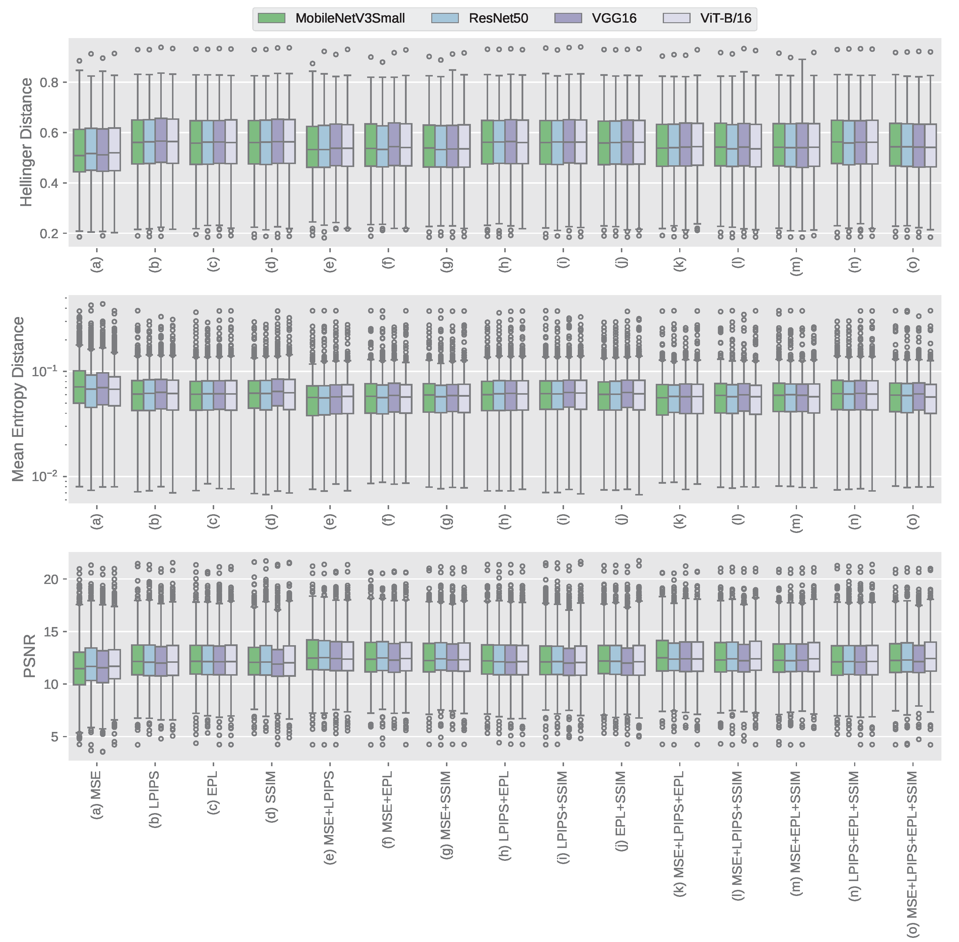
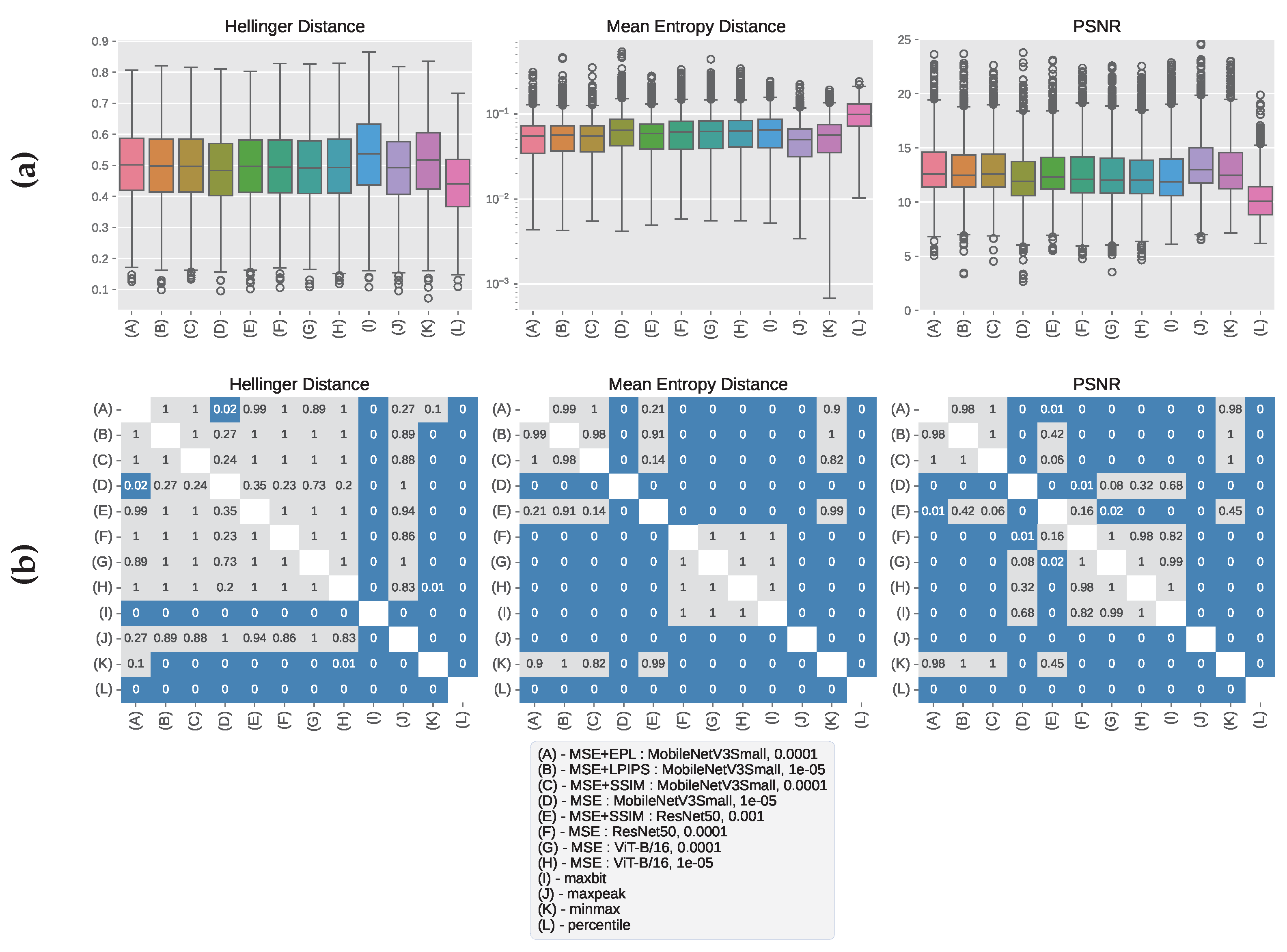
3.1. CHC Rijeka Results

The following results correspond to the CHC Rijeka test set. Models identified as Pareto-optimal based on validation performance were evaluated and compared against the maxbit, minmax, percentile, and maxpeak scaling methods described in the baseline study [23]. The test set results are presented in Figure 5, where each scaling method is abbreviated with an uppercase character for brevity. In contrast to the performance shown in Figure 4 (where there were no obvious differences between the architectures), none of the Pareto-optimal models (shown in Figure 5a) were based on VGG16. Instead, they predominantly used the MobileNetV3Small architecture. Furthermore, all of the Pareto-optimal models included MSE as a part of the loss function. This further confirms that the best-performing models leveraged the original window parameters as a strong starting point, which were then refined using additional loss functions (EPL, LPIPS, and SSIM). On the other hand, none of the Pareto-optimal models combined more than two losses, suggesting that, for example, using MSE+LPIPS+EPL did not offer any additional benefit over using MSE+EPL or MSE+LPIPS.

While observing the results in Figure 5a, it can be seen that percentile scaling attained the lowest Hellinger distance but also the highest average MED and lowest average PSNR. This suggests that percentile scaling preserved the pixel value distributions, but at the cost of overall image quality and consistency. In contrast, scaling with maxbit or minmax resulted in higher Hellinger distances than percentile but also better MED and PSNR scores, indicating better structural preservation over percentile. Among the other tested methods, the trained ML models ((A), (B), (C), (D), (E), (F), (G), and (H)) showed balanced performance across all three metrics, as did maxpeak, with the latter having also attained the best overall peak-signal-to-noise ratio. These trends are supported by statistical analysis. The ANOVA test indicated potential significant differences between methods, and the results of Tukey HSD tests (Figure 5b) confirm that percentile scaling was significantly different from all other methods across all three metrics. Furthermore, maxpeak’s PSNR and MED scores were statistically different than all the other tested methods. Methods (A), (C), and (E) performed similarly to (B), with no statistical differences, and a similar trend is observable in methods (F), (G), and (H), where p > 0.9 across all three metrics.

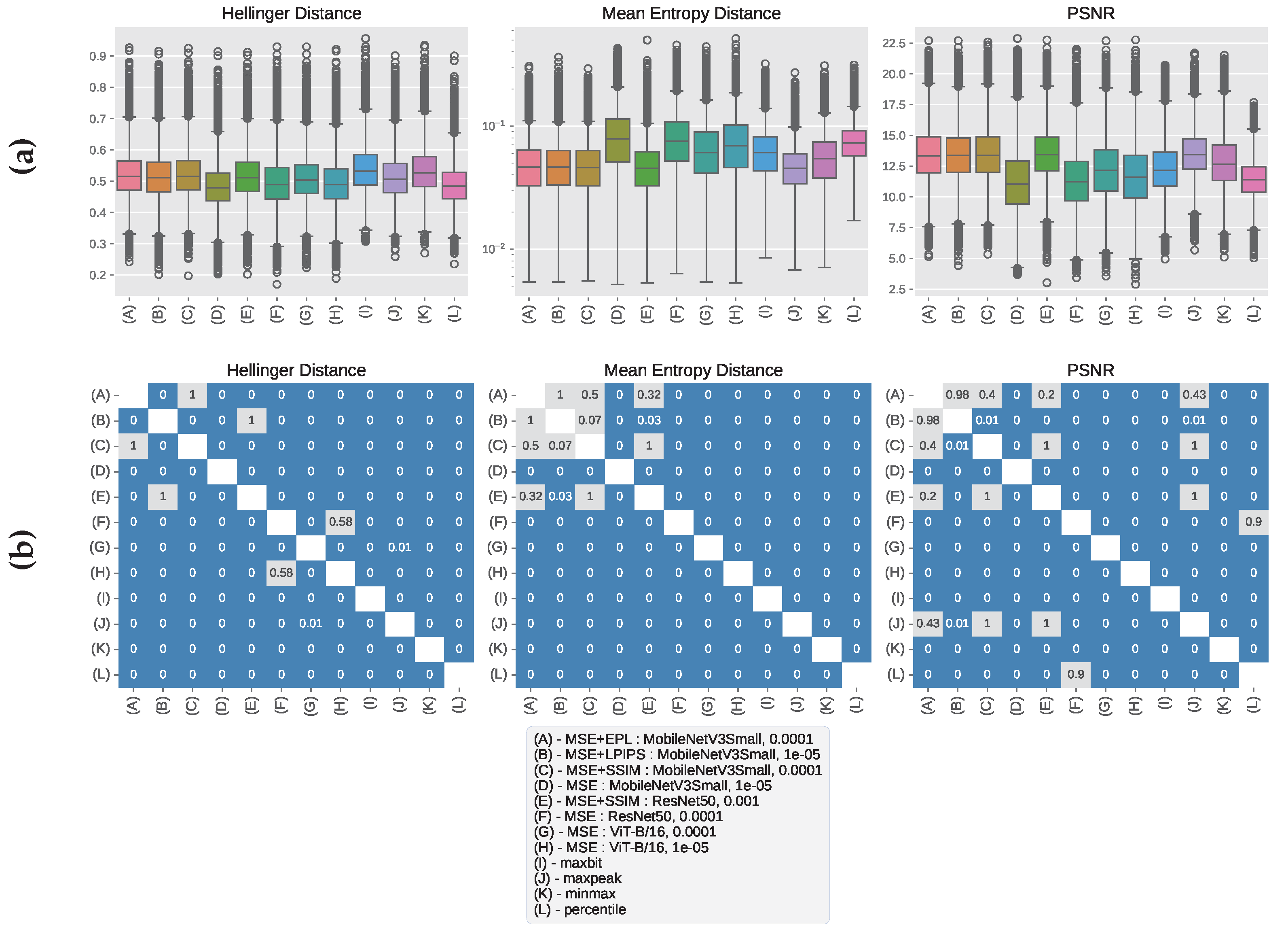
3.2. GRAZPEDWRI-DX Results

Models trained on the CHC Rijeka dataset were directly applied to the GRAZPEDWRI-DX images to predict windowing parameters. The results are given in Figure 6, where (a) shows the performance across the three tested metrics (Hellinger distance, MED, PSNR), and (b) shows the statistical differences across method pairs.

The results shown in Figure 6a demonstrate greater variability across the three evaluation metrics compared with the results presented in Figure 5a. While this could partially be attributed to the larger size of GRAZPEDWRI-DX (over 20,000 images versus ≈2000 in the CHC Rijeka test set), it is also likely influenced by dataset composition. Although the training data and GRAZPEDWRI-DX differ in bit depth (CHC Rijeka images being mostly 12-bit and GRAZPEDWRI-DX images being 16-bit) this likely had minimal impact on the predictions, as all images were normalised prior to inference. However, there is a clear difference in anatomical regions present in both datasets: the original data include a variety of anatomical regions (as shown in Figure 2), and GRAZPEDWRI-DX contains only wrist radiographs. It is likely that the combination of a larger dataset and a different scope of anatomical regions in GRAZPEDWRI-DX amplified performance differences between methods and, as a result, statistical comparisons revealed significant differences across nearly all method pairs and metrics. The only methods that showed no statistically significant differences across all three metrics were methods (A) and (C), indicating that their performance was statistically similar on the GRAZPEDWRI-DX dataset. Methods (B) and (E) also shared some similarities with (A) and (C) across MED and PSNR, but obtained significantly different Hellinger distances.

3.3. Qualitative Analysis of Windowed Image Outputs

Figure 7 shows visual examples of windowed images. For brevity, methods such as (A), (C), and (E) are omitted due to their statistically similar performance to (B), and method (G) for its similar performance to (H) on the CHC Rijeka test set. In some cases, nearly all methods produced acceptable outputs (Figure 7a). However, images scaled using percentile occasionally overcropped pixel values, leading to information loss in areas showing tissue, as seen in Figure 7b–d. Conversely, minmax and maxbit retained a significant amount of irrelevant information, particularly air surrounding the anatomical region, and in some instances, even resulted in information loss within the body region itself (Figure 7b). The maxpeak method consistently preserved more relevant information than minmax, maxbit, and percentile, which explains its high PSNR and low MED. This is evident in Figure 7b, with maxpeak scaling resulting in an image where none of the relevant image areas exhibit high information loss, and the minor information loss can primarily be attributed to noise.

Methods (D), (F), and (H), which learned to scale images only using window parameters found in DICOM, were the most effective at removing pixel values from irrelevant image regions (e.g., surrounding air) while maintaining tissue integrity, as seen across Figure 7b–d. However, this approach resulted in a higher entropy distance (MED), as non-anatomical regions lost nearly all entropy (thus increasing MED, as evident in Figure 6a). This also explains the greater variability in performance, which was observed between Figure 5 and Figure 6, as wrist radiographs (such as the ones from the GRAZPEDWRI-DX dataset) typically contain larger regions of air compared with chest radiographs, which are prevalent in the CHC Rijeka dataset. A good example of non-anatomical region size differences can be observed in Figure 7a (from CHC Rijeka test set) and Figure 7c (from GRAZPEDWRI-DX).

In contrast to (D), (F), and (H), methods (A), (B), (C), and (E), which built upon the original windowing parameters by using an auxiliary loss function, presented a more balanced approach. These window scaling methods cropped out irrelevant image regions (e.g., air, although less severely than methods (D), (F), and (H)) while still retaining sufficient information in important areas (Figure 7c,d). Images windowed using these approaches were mostly similar to maxpeak, but there were also instances where these methods were better at preserving tissue-area pixels (e.g., the difference between (B) and maxpeak in Figure 7c).

4. Discussion

There is no definitive “best” method for this problem, as each approach has its strengths and weaknesses. The appeal of maxpeak, minmax, maxbit, and percentile lies in their simplicity. With minimal hyperparameter tuning, these methods require no training and are readily applicable out-of-the-box. Among them, maxpeak stands out as the most effective at preserving relevant pixel values. Though not perfect, it is lightweight and performs well in most cases, requiring only simple hyperparameter adjustments.

The trained neural networks demonstrated good visual preservation of critical image areas and removing pixel values that primarily represented air (considered noise). This highlights a key advantage of learning-based methods—their ability to selectively remove irrelevant information while preserving important image details. The tested ML models were also found to be adaptable to 16-bit DICOM images, despite the majority of the training data ($97.1\%$) consisting of 12-bit images. This highlights the importance of pixel value normalization and paying attention to varying bit-depth distributions in medical imaging. As illustrated in Figure 7a,c,d, the predicted windowing parameters successfully preserved the anatomical region in a 16-bit image, with the greatest information loss visible in background areas (air), which are typically less relevant for clinical interpretation.

Although several additional objectives (EPL, LPIPS, SSIM) were tested as auxiliary losses during training—individually (on their own)—these losses were not as good in preserving critical image information. This is evidenced by all Pareto-optimal models, including the MSE loss, which affirms its role in providing a strong foundation for preserving critical information in windowed images. Also, no Pareto-optimal model used more than two auxiliary losses, suggesting that including multiple auxiliary losses provided no further benefit beyond pairing a single auxiliary loss with MSE. While other losses could be explored in future research, testing them falls outside the scope of this study.

Although ML models can typically handle high bit-depth inputs, the predicted window parameters may also benefit downstream ML tasks by enhancing contrast and reducing noise. This could potentially impact performance in applications such as classification or segmentation, akin to how focusing on uniform patterns (and ignoring non-uniform patterns) improves classification accuracy in fluorescence microscopy images [44,45]. Therefore, future work could explore the use of predicted windowing parameters as a preprocessing step in downstream medical ML tasks [6,7,8,9], as windowing inherently changes the luminance distribution in DICOM images (as visible in Figure 7).

5. Conclusions

Ultimately, the choice of method depends on the specific application. For general-purpose use, maxpeak offers a fast, robust, easily deployable solution with reliable performance in preserving X-ray image information. However, for scenarios where preserving anatomical structures and removing noise is important, trained ML models provide an advantage in selectively filtering out noise while maintaining tissue details.

The current study is limited to CR images and does not incorporate any context (i.e., DICOM metadata) into its predictions, which may limit its applicability in more complex medical imaging modalities, such as CT, where windowing depends heavily on the diagnostic aim and the target tissue. Future work may address these limitations by extending the proposed framework to CT imaging and leveraging metadata (e.g., the BodyPartExamined attribute) to enable context-aware parameter prediction. Further exploration of alternative auxiliary loss functions (beyond what is tested in this study) may also enhance the preservation of diagnostically relevant information during bit-depth compression. Another interesting direction for future work would be to investigate whether different windowing strategies influence the performance of downstream ML models, e.g., whether two identically trained models perform differently when using 8-bit inputs scaled via different windowing methods.

References

1. Mildenberger, P.; Eichelberg, M.; Martin, E. Introduction to the DICOM standard. Eur. Radiol. 2001, 12, 920–927. [Google Scholar] [CrossRef] [PubMed]
2. Mustra, M.; Delac, K.; Grgic, M. Overview of the DICOM standard. In Proceedings of the 2008 50th International Symposium ELMAR, Zadar, Croatia, 10–12 September 2008; Volume 1, pp. 39–44. [Google Scholar]
3. Kimpe, T.; Tuytschaever, T. Increasing the Number of Gray Shades in Medical Display Systems—How Much is Enough? J. Digit. Imaging 2006, 20, 422–432. [Google Scholar] [CrossRef]
4. Hosny, A.; Parmar, C.; Quackenbush, J.; Schwartz, L.H.; Aerts, H.J.W.L. Artificial intelligence in radiology. Nat. Rev. Cancer 2018, 18, 500–510. [Google Scholar] [CrossRef]
5. Chan, H.P.; Hadjiiski, L.M.; Samala, R.K. Computer-aided diagnosis in the era of deep learning. Med. Phys. 2020, 47, e218–e227. [Google Scholar] [CrossRef]
6. Ali, S.; Li, J.; Pei, Y.; Khurram, R.; ur Rehman, K.; Mahmood, T. A Comprehensive Survey on Brain Tumor Diagnosis Using Deep Learning and Emerging Hybrid Techniques with Multi-modal MR Image. Arch. Comput. Methods Eng. 2022, 29, 4871–4896. [Google Scholar] [CrossRef]
7. Radiya, K.; Joakimsen, H.L.; Mikalsen, K.Ø.; Aahlin, E.K.; Lindsetmo, R.O.; Mortensen, K.E. Performance and clinical applicability of machine learning in liver computed tomography imaging: A systematic review. Eur. Radiol. 2023, 33, 6689–6717. [Google Scholar] [CrossRef] [PubMed]
8. Islam, M.R.; Nahiduzzaman, M. Complex features extraction with deep learning model for the detection of COVID19 from CT scan images using ensemble based machine learning approach. Expert Syst. Appl. 2022, 195, 116554. [Google Scholar] [CrossRef]
9. Wu, G.; Wang, Z.; Peng, J.; Gao, S. Coarse-to-Fine bone age regression by using multi-scale self-attention mechanism. Biomed. Signal Process. Control 2025, 100, 107029. [Google Scholar] [CrossRef]
10. Singh, D.; Singh, B. Investigating the impact of data normalization on classification performance. Appl. Soft Comput. 2020, 97, 105524. [Google Scholar] [CrossRef]
11. Morán-Fernández, L.; Sechidis, K.; Bolón-Canedo, V.; Alonso-Betanzos, A.; Brown, G. Feature selection with limited bit depth mutual information for portable embedded systems. Knowl.-Based Syst. 2020, 197, 105885. [Google Scholar] [CrossRef]
12. Pawar, K.; Chen, Z.; Shah, N.J.; Egan, G.F. A Deep Learning Framework for Transforming Image Reconstruction Into Pixel Classification. IEEE Access 2019, 7, 177690–177702. [Google Scholar] [CrossRef]
13. Yeganeh, H.; Wang, Z.; Vrscay, E.R. Adaptive Windowing for Optimal Visualization of Medical Images Based on a Structural Fidelity Measure. In Image Analysis and Recognition; Springer: Berlin/Heidelberg, Germany, 2012; pp. 321–330. [Google Scholar] [CrossRef]
14. Gao, S.; Han, W.; Ren, Y.; Li, Y. High Dynamic Range Image Rendering with a Luminance-Chromaticity Independent Model. In Intelligence Science and Big Data Engineering. Image and Video Data Engineering; Springer International Publishing: Cham, Switzerland, 2015; pp. 220–230. [Google Scholar] [CrossRef]
15. Echabbi, K.; Zemmouri, E.; Douimi, M.; Hamdi, S. A General Preprocessing Pipeline for Deep Learning on Radiology Images: A COVID-19 Case Study. In Progress in Artificial Intelligence; Springer International Publishing: Cham, Switzerland, 2022; pp. 232–241. [Google Scholar] [CrossRef]
16. Rudolph, J.; Schachtner, B.; Fink, N.; Koliogiannis, V.; Schwarze, V.; Goller, S.; Trappmann, L.; Hoppe, B.F.; Mansour, N.; Fischer, M.; et al. Clinically focused multi-cohort benchmarking as a tool for external validation of artificial intelligence algorithm performance in basic chest radiography analysis. Sci. Rep. 2022, 12, 12764. [Google Scholar] [CrossRef] [PubMed]
17. Skurowski, P.; Wicher, K. High Dynamic Range in X-ray Imaging. In Information Technology in Biomedicine; Springer International Publishing: Cham, Switzerland, 2018; pp. 39–51. [Google Scholar] [CrossRef]
18. Lederer, A.; Kunzelmann, K.; Hickel, R.; Litzenburger, F. Transillumination and HDR Imaging for Proximal Caries Detection. J. Dent. Res. 2018, 97, 844–849. [Google Scholar] [CrossRef]
19. Murphy, A.; Feger, J.; Ismail, M.A. Windowing (CT). 2017. Available online: https://radiopaedia.org/articles/52108 (accessed on 1 May 2025).
20. Masoudi, S.; Harmon, S.A.A.; Mehralivand, S.; Walker, S.M.; Raviprakash, H.; Bagci, U.; Choyke, P.L.; Turkbey, B. Quick guide on radiology image pre-processing for deep learning applications in prostate cancer research. J. Med. Imaging 2021, 8, 010901. [Google Scholar] [CrossRef]
21. Mangone, M.; Diko, A.; Giuliani, L.; Agostini, F.; Paoloni, M.; Bernetti, A.; Santilli, G.; Conti, M.; Savina, A.; Iudicelli, G.; et al. A Machine Learning Approach for Knee Injury Detection from Magnetic Resonance Imaging. Int. J. Environ. Res. Public Health 2023, 20, 6059. [Google Scholar] [CrossRef] [PubMed]
22. Zhao, X.; Zhang, T.; Liu, H.; Zhu, G.; Zou, X. Automatic Windowing for MRI With Convolutional Neural Network. IEEE Access 2019, 7, 68594–68606. [Google Scholar] [CrossRef]
23. Hržić, F.; Napravnik, M.; Baždarić, R.; Štajduhar, I.; Mamula, M.; Miletić, D.; Tschauner, S. Estimation of Missing Parameters for DICOM to 8-bit X-ray Image Export. In Proceedings of the 2022 International Conference on Electrical, Computer, Communications and Mechatronics Engineering (ICECCME), Maldives, Maldives, 16–18 November 2022; pp. 1–6. [Google Scholar]
24. Suganyadevi, S.; Seethalakshmi, V.; Balasamy, K. A review on deep learning in medical image analysis. Int. J. Multimed. Inf. Retr. 2021, 11, 19–38. [Google Scholar] [CrossRef]
25. Mikulić, M.; Vičević, D.; Nagy, E.; Napravnik, M.; Štajduhar, I.; Tschauner, S.; Hržić, F. Balancing Performance and Interpretability in Medical Image Analysis: Case study of Osteopenia. J. Imaging Inform. Med. 2024, 38, 177–190. [Google Scholar] [CrossRef]
26. Chowdhury, M.E.H.; Rahman, T.; Khandakar, A.; Mazhar, R.; Kadir, M.A.; Mahbub, Z.B.; Islam, K.R.; Khan, M.S.; Iqbal, A.; Emadi, N.A.; et al. Can AI Help in Screening Viral and COVID-19 Pneumonia? IEEE Access 2020, 8, 132665–132676. [Google Scholar] [CrossRef]
27. Morid, M.A.; Borjali, A.; Del Fiol, G. A scoping review of transfer learning research on medical image analysis using ImageNet. Comput. Biol. Med. 2021, 128, 104115. [Google Scholar] [CrossRef]
28. Abbaoui, W.; Retal, S.; Ziti, S.; El Bhiri, B. Automated Ischemic Stroke Classification from MRI Scans: Using a Vision Transformer Approach. J. Clin. Med. 2024, 13, 2323. [Google Scholar] [CrossRef]
29. Napravnik, M.; Hržić, F.; Tschauner, S.; Štajduhar, I. Building RadiologyNET: An unsupervised approach to annotating a large-scale multimodal medical database. BioData Min. 2024, 17, 22. [Google Scholar] [CrossRef] [PubMed]
30. Choplin, R.H.; J M Boehme, N.; Maynard, C.D. Picture archiving and communication systems: An overview. RadioGraphics 1992, 12, 127–129. [Google Scholar] [CrossRef]
31. Sobel, I.; Feldman, G. A 3×3 isotropic gradient operator for image processing. Pattern Classif. Scene Anal. 1973, 271–272. [Google Scholar]
32. Brunet, D.; Vrscay, E.R.; Wang, Z. On the Mathematical Properties of the Structural Similarity Index. IEEE Trans. Image Process. 2012, 21, 1488–1499. [Google Scholar] [CrossRef] [PubMed]
33. Zhao, H.; Gallo, O.; Frosio, I.; Kautz, J. Loss Functions for Image Restoration With Neural Networks. IEEE Trans. Comput. Imaging 2017, 3, 47–57. [Google Scholar] [CrossRef]
34. Zhang, R.; Isola, P.; Efros, A.A.; Shechtman, E.; Wang, O. The Unreasonable Effectiveness of Deep Features as a Perceptual Metric. In Proceedings of the IEEE Conference on Computer Vision and Pattern Recognition (CVPR), Salt Lake City, UT, USA, 18–23 June 2018. [Google Scholar]
35. Ding, K.; Ma, K.; Wang, S.; Simoncelli, E.P. Comparison of Full-Reference Image Quality Models for Optimization of Image Processing Systems. Int. J. Comput. Vis. 2021, 129, 1258–1281. [Google Scholar] [CrossRef]
36. Chang, Q.; Li, X.; Li, Y.; Miyazaki, J. Multi-directional Sobel operator kernel on GPUs. J. Parallel Distrib. Comput. 2023, 177, 160–170. [Google Scholar] [CrossRef]
37. Krizhevsky, A.; Sutskever, I.; Hinton, G.E. ImageNet Classification with Deep Convolutional Neural Networks. Commun. ACM 2017, 60, 84–90. [Google Scholar] [CrossRef]
38. Loshchilov, I.; Hutter, F. Fixing Weight Decay Regularization in Adam. arXiv 2017, arXiv:1711.05101. [Google Scholar] [CrossRef]
39. Yu, T.; Kumar, S.; Gupta, A.; Levine, S.; Hausman, K.; Finn, C. Gradient Surgery for Multi-Task Learning. In Advances in Neural Information Processing Systems; Larochelle, H., Ranzato, M., Hadsell, R., Balcan, M., Lin, H., Eds.; Curran Associates, Inc.: Sydney, NSW, Australia, 2020; Volume 33, pp. 5824–5836. [Google Scholar]
40. Wu, Y.; Zhou, Y.; Saveriades, G.; Agaian, S.; Noonan, J.P.; Natarajan, P. Local Shannon entropy measure with statistical tests for image randomness. Inf. Sci. 2013, 222, 323–342. [Google Scholar] [CrossRef]
41. González-Castro, V.; Alaiz-Rodríguez, R.; Alegre, E. Class distribution estimation based on the Hellinger distance. Inf. Sci. 2013, 218, 146–164. [Google Scholar] [CrossRef]
42. Al-Shaykh, O.; Mersereau, R. Lossy compression of noisy images. IEEE Trans. Image Process. 1998, 7, 1641–1652. [Google Scholar] [CrossRef]
43. Nagy, E.; Janisch, M.; Hržić, F.; Sorantin, E.; Tschauner, S. A pediatric wrist trauma X-ray dataset (GRAZPEDWRI-DX) for machine learning. Sci. Data 2022, 9, 222. [Google Scholar] [CrossRef] [PubMed]
44. Fekri-Ershad, S. Cell phenotype classification using multi threshold uniform local ternary patterns in fluorescence microscope images. Multimed. Tools Appl. 2021, 80, 12103–12116. [Google Scholar] [CrossRef]
45. Fekri-Ershad, S.; Ramakrishnan, S. Cervical cancer diagnosis based on modified uniform local ternary patterns and feed forward multilayer network optimized by genetic algorithm. Comput. Biol. Med. 2022, 144, 105392. [Google Scholar] [CrossRef]
Figure 1. A flowchart of steps taken to transform a CR image from 12 to 8 bits. After windowing is performed, the image is stored in 8-bit format, and its highest pixel value is 255.
Mathematics 13 01596 g001
Figure 2. Distribution of the dataset used for this study within the training, validation, and test sets. Subplots depict the distribution of (a) dataset splits and (b) anatomical regions within each subset.
Mathematics 13 01596 g002
Figure 3. Losses used during training with two example inputs: example (1) shows an image windowed using satisfactory predictions, and example (2) demonstrates excessive clipping due to poorly predicted windowing parameters.
Mathematics 13 01596 g003
Figure 4. Performance of ML models (with different loss functions) on the validation set. Lower values indicate better performance for Hellinger distance and Mean Entropy Distance (MED), while higher values are better for PSNR. MED is displayed on a logarithmic scale, whereas PSNR and Hellinger distance are shown on linear scales.
Mathematics 13 01596 g004
Figure 5. (a) Performance of windowing methods on the test set. MED is displayed on a logarithmic scale, while PSNR and Hellinger distance are shown on linear scales. (b) Statistical comparisons between windowing methods using Tukey’s Honest Significant Difference (HSD) tests. Significant differences (p < 0.05) between method pairs are indicated in blue.
Mathematics 13 01596 g005
Figure 6. (a) Performance of windowing methods on the GRAZPEDWRI-DX dataset. MED is displayed on a logarithmic scale, while PSNR and Hellinger distance are shown on linear scales. (b) Statistical comparisons between windowing methods using Tukey’s Honest Significant Difference (HSD) tests. Significant differences (p < 0.05) between method pairs are indicated in blue.
Mathematics 13 01596 g006
Figure 7. Results of 8-bit DICOM export after windowing. In each subfigure, the top row shows the raw image and its windowed counterparts; the second row shows the local pixel entropy of the corresponding image in the top row (darker regions → lower entropy, brighter regions → higher entropy); and the bottom row shows the entropy difference between the raw image and each windowed version. Windows predicted by each method are displayed above the top row as WC (WindowCenter) and WW (WindowWidth). The minimum and maximum pixel values from the raw image are indicated above the leftmost image in the top row. Subfigures (a,b) are from the CHC Rijeka test set, while (c,d) are from the GRAZPEDWRI-DX dataset.
Mathematics 13 01596 g007
Disclaimer/Publisher’s Note: The statements, opinions and data contained in all publications are solely those of the individual author(s) and contributor(s) and not of MDPI and/or the editor(s). MDPI and/or the editor(s) disclaim responsibility for any injury to people or property resulting from any ideas, methods, instructions or products referred to in the content.