Robustness Study of Unit Elasticity of Intertemporal Substitution Assumption and Preference Misspecification

Abstract

This paper proposes a novel robustness framework for studying the unit elasticity of intertemporal substitution (EIS) assumption based on the Perron-Frobenius sieve estimation model by Christensen, 2017. The sieve nonparametric decomposition is a central model that connects key strands of the long run risk literature and recovers the stochastic discount factor (SDF) under the unit EIS assumption. I generate various economies based on Epstein–Zin preferences to simulate scenarios where the EIS deviates from unity. Then, I study the main estimation mechanism of the decomposition as well as the time discount factor and the risk aversion parameter estimation surface. The results demonstrate the robustness of estimating the average yield, change of measure, and preference parameters but also reveal an “absorption effect” arising from the unit EIS assumption. The findings highlight that asset pricing models assuming a unit EIS produce distorted parameter estimates, caution researchers about the potential under- or over-estimation of risk aversion, and provide insight into trends of misestimation when interpreting the results. I also identify an additional source of failure from a consumption component, which demonstrates a more general limit of the consumption-based capital asset pricing model and the structure used to estimate relevant preference parameters.

1. Introduction

Asset pricing theory has long emphasized the importance of correctly modeling investors’ preferences for risk and intertemporal substitution. The recursive preferences developed by Epstein and Zin [1] broke this tight link by allowing risk aversion to be distinct from the elasticity of intertemporal substitution (EIS). This innovation enabled models to jointly accommodate reasonable consumption-smoothing behavior and high-risk premia. Notably, the long-run risk framework of Bansal and Yaron [2] relies on an EIS greater than one to generate sizable equity premiums without resorting to extreme risk aversion. Meanwhile, estimating the stochastic discount factor (SDF) is crucial in macro finance because of the relevant preference information included in the SDF. The difficulty of recovering the SDF makes how to estimate the SDF a substantial problem. Hansen and Scheinkman [3] propose a theoretical model through the Perron–Frobenius problem approach to obtain a clearer expression of the decomposition for the stochastic discount factor. From what they find, the permanent and transitory components can be expressed using the SDF, Perron–Frobenius eigenfunction, and its corresponding eigenvalue.

Later, Christensen [4] provides an econometrics model to estimate the eigenfunction, eigenvalue, and SDF decomposition using the sieve model. Christensen [4] assumes unity EIS for the recursive value function, which yields analytical convenience. This is a notable restriction because a large empirical literature suggests that the EIS often deviates substantially from unity in reality. Then, an interesting question is “whether the sieve method is robust when the EIS is not unity and what preference information is misspecified”. Moreover, because the unit-EIS assumption remains ubiquitous across a wide range asset pricing models, addressing this question carries broad relevance. In this paper, I propose a novel robustness study design and study the unit EIS assuming sieve estimation when feeding non-unit EIS-generated data.

My proposed robustness framework starts with applying the Tauchen and Hussey [5] and Smith [6] methods in the data-generating process (DGP). By choosing different time discount factors, risk aversion parameters, and a non-unit EIS, the corresponding economies are obtained, which generate different asset returns. In the first part of estimating the eigenfunction and eigenvalue, the consumption and dividend growth rates follow the quadrature process proposed by Tauchen and Hussey [5]. In the second step of estimating the SDF decomposition, following the Smith [6] and Tauchen and Hussey [5] setup, asset returns data can be computed using consumption and dividend growth rate, which were generated in the first step. The key estimation steps in Christensen [4] were replicated using the newly generated data. The estimated eigenfunction, eigenvalue, and the change of measure are similar to those in Christensen [4]. The estimated eigenfunctions are flat and take reasonable values. The estimated change of measure is close to what theories suggest. Furthermore, the permanent component in the SDF was shown to follow the martingale property under the condition of non-unit EIS.

Then, the robustness study of the Perron–Frobenius sieve estimation is discussed by studying the surface of the objective function according to different parameters. More specifically, I study the surface for estimating the time discount factor ($\beta$) and risk aversion parameter ($\gamma$) when the EIS is not one. The surface for estimating $\beta$ is well behaved and concave. The surface for estimating $\gamma$ is also concave around 20. However, the estimated $\gamma$ deviates a lot from its true value. Christensen [4] concludes the same poor estimation result for $\gamma$ when the EIS is assumed to be one. But the author does not mention the reason. By inspecting the objective-function surface for $\gamma$ in a neighborhood of its data-generating value, I show that this surface is non-concave. The study of the component decomposition of the objective function identifies the source of this non-concavity and exposes a broader limitation of the consumption-based asset-pricing model. I also demonstrate that imposing the unit EIS when the true economy has an EIS $\ne 1$ leads to a distortion in the estimated preference parameters. The risk aversion coefficient can be substantially misestimated to “compensate” for the misspecified EIS. The findings highlight a subtle but important form of identification failure that I term an “absorption effect”. When the true EIS differs from one but the model fixes it at unity, the estimation procedure compensates by misidentifying the risk aversion coefficient. In the experiments, the agent’s relative risk aversion absorbs the misspecification in intertemporal substitution. The sieve estimator still fits asset price dynamics well, but it does so by attributing excess smoothness or impatience to a distorted risk aversion estimate. Additionally, the consumption growth rate component in the objective function grows rapidly when $\gamma$ gets larger. The factor causing models to fail to estimate $\gamma$ precisely is the limitation of the consumption-based asset pricing model.

These findings underscore that the identification of risk aversion in asset pricing models is fundamentally compromised by fixing the misspecified EIS value. The model will fit the data by warping the risk aversion parameter. I highlight a broader lesson for the related literature because the analysis is situated in the context of recursive utility and long-run risk models. Empirical implementations of asset pricing models must carefully interpret estimated parameters with the unit EIS assumption. The results thus bridge an important gap between the theoretical appeal of Epstein–Zin preferences and the practical estimation of SDFs and illustrate how the unit EIS assumption can impact the robustness to recover agents’ risk preferences. However, there is stability in estimating time discount factor parameters under this assumption. I detail the theoretical intuition for the absorption effect, present the simulation-based robustness exercises, and discuss the implications of the results in light of related empirical findings.

2. Materials and Methods

2.1. Motivations

2.1.1. The Elasticity of Intertemporal Substitution and the Challenges

The elasticity of intertemporal substitution measures how willing consumers are to shift their consumption over time in response to changes in the real rate of return. Mathematically, for a utility function, the EIS can be derived from the negative ratio of the log change in consumption growth to the log change in the marginal utility of consumption. The EIS is relevant in both macroeconomics and finance because a higher EIS implies a more aggressive reallocation toward future consumption when returns rise, whereas a lower EIS means relatively inelastic responses.

The effect of the EIS on one economy can be summarized in the following aspects. The EIS affects the consumption growth rate directly from its definition and original intuition—the EIS determines how much consumers change their expected consumption growth rate in response to changes in the expected return to any such asset [7]. Campbell and Viceira [8] find that the EIS is the key parameter of the consumption choice in solving the consumption and asset portfolio decision problem. Browning and Crossley [9] study an empirical estimation model and point out that the EIS is the coefficient of asset returns concluding information from individuals’ substitution of consumption over time.

The EIS can also be described as a function of the unobservable continuation value of the future consumption plan which captures important individuals’ behavior preferences. In any recursive utility model, the different EIS will alter the estimates of the value function then affect the interpretation of the implications for the asset returns. The third aspect of the interpretation from the EIS was studied in a sequence of the literature on long-run risk models. This sequence of the literature is a specific model of cash flow dynamics following from the intertemporal composition of risk. Bansal and Yaron [2] explain the risk premium and high Sharpe ratios observed in U.S. data by assuming there exists a small, persistent, and predictable component (long-run risk) in consumption and dividend growth. Campbell [10] states that the long-run risk component can help rationalize those observations by specializing the relationship between risk aversion and EIS.

Despite the theoretical importance of the EIS, estimating the EIS precisely remains a significant empirical challenge. One source of difficulty lies in the smooth nature of aggregate consumption data, which provides limited variation for identifying how consumers respond to changes in the real rate of return. Hall [11] finds small or even near-zero EIS estimates, in part because the time series on consumption and interest rates offer insufficient volatility to capture how strongly households might shift consumption over time. In addition, relying on lower-frequency data (e.g., annual or quarterly) can mask short-term consumption adjustments, especially among households influenced by liquidity constraints or precautionary saving motives [12].

Model specification likewise complicates the task. Many empirical tests rely on standard time-additive preferences, which constrain risk aversion and the EIS to be inversely related. Frameworks, such as Epstein–Zin preferences [1] and long-run risk models [2], relax this restriction. These advanced models can better match observed asset returns and consumption patterns but also introduce additional parameters, state variables, or unobservable components that make estimation more demanding.

2.1.2. The Unit EIS Assumption and the Modeling Issues

a.

The EIS in Epstein–Zin Preferences

The Consumption-Based Capital Asset Price Model (CCAPM) [13] has been popular because it explicitly shows how an asset’s risk premium arises from its covariance with consumption growth, thereby unifying portfolio choices and intertemporal consumption decisions under uncertainty. However, there are limitations, as findings from the CCAPM have been rejected in various empirical settings [14,15]. The CCAPM fails to explain the equity premium puzzle, the high volatility of the stock market compared with relatively stable interest rates, and the predictability of excess stock market returns. In response, researchers have introduced new models to improve the CCAPM. Epstein and Zin [1] propose recursive utility specifications that break the tight link between the coefficient of relative risk aversion and the inverse of the EIS. By allowing these two parameters to vary independently, they demonstrate how asset returns depend jointly on households’ aversion to risk and their willingness to shift consumption across time and offer deeper insights into how risk premia arise from fluctuations in consumption and marginal utility.

Epstein and Zin [1] define the recursive utility function when the Bellman equation takes the form

$$V_t=\{(1-\beta )c_t^{1-\theta }+\beta \mathbb{E}{\left[V_{t+1}^{1-\gamma }\right|{\mathcal{F}}_t]}^{{\displaystyle \frac{1-\theta }{1-\gamma }}}{\}}^{{\displaystyle \frac{1}{1-\theta }}},$$

(1)

where $V_t$ is the value function, $c_t$ is the consumption in period t, $\beta \in (0,1)$ is the time discount factor, $\gamma$ is the relative risk aversion parameter, $1/\theta$ is the EIS, and ${\mathcal{F}}_t$ is the information known up to period t. In this framework, risk aversion and the EIS become independent parameters, allowing one to break the tight link that arises in standard expected-utility models.

b.

The Empirical Evidence of Non-Unit EIS

Both the theoretical and empirical works find that the EIS is usually significantly different from one. Hall [11] finds that consumption growth barely responds to real interest rates, implying an EIS near zero. Campbell and Mankiw [16] report that predictable income changes drive consumption more than interest rate movements, consistent with roughly half of households behaving as “rule-of-thumb” consumers who effectively have zero EIS. That said, later work uncovered heterogeneity. Using micro-panel data, Attanasio and Weber [17,18] estimates a larger EIS, around 0.3 in aggregates and up to 0.8 when controlling for cohort effects, once aggregation biases are addressed. The EIS appears higher for wealthier, more financially active households. In their results, stock market participants have an EIS around 0.3–0.4, versus 0.8–1 for bondholders, and the EIS tends to rise with household wealth. Campbell and Mankiw [16] provide further empirical support indicating substantial heterogeneity in intertemporal substitution behavior across the population, even though the average EIS is often below one.

Several household-level studies, especially focusing on wealthy consumers and active investors, have found EIS estimates at or above one. Vissing-Jørgensen [19] shows that accounting for asset market participation raises the estimated EIS: stockholders have an EIS around 0.3–0.4, whereas bondholders who hold safe assets have an EIS in the 0.8–1 range, with an even higher EIS for the wealthiest asset-holding households. In a follow-up, Vissing-Jørgensen and Attanasio [20] estimate Euler equations for different assets and find that stockholding households exhibit an EIS of roughly 1.4 when measured from treasury bill returns and about 0.4 when using stock returns. This implies that active investors and wealthy households can have an EIS well above one, consistent with greater willingness to shift consumption intertemporally. Likewise, Attanasio and Weber [18] use microconsumption data and control for demographics to estimate the EIS and find an EIS with values greater than one.

c.

The Rationale and Limitations of the Unit EIS Assumption

Despite theoretical and empirical evidence showing that EISs are usually non-unit, many macroeconomic models set the EIS $=1$ with logarithmic utility for tractability and consistency with balanced growth. Pioneering real business cycle papers exemplify this approach. The Lucas [21] asset pricing model and Kydland and Prescott [22] equilibrium growth model both employ log utility, which yields convenient analytical solutions and stable steady states. In particular, King et al. [23] note that setting the constant relative risk aversion (CRRA) curvature where risk aversion and the EIS are both equal to 1 is required to obtain a balanced growth path when preferences are additively separable in consumption and leisure. When the EIS $=1$, the Euler equation simplifies as consumption growth depends linearly on the interest rate gap, which greatly eases the model solution and calibration.

Assuming the EIS $=1$ when the true elasticity differs can distort model predictions in both macroeconomics and finance. In macro models, assuming a unit EIS is too high relative to empirically estimated values, which are typically well below one, overstates consumers’ willingness to reallocate consumption over time, thereby exaggerating the sensitivity of consumption to changes in interest rates. This misspecification can lead policymakers astray. For example, a New Keynesian model with an EIS $=1$ may predict a larger consumption boom from a rate cut than would occur if households were, in fact, more reluctant to substitute consumption intertemporally. Conversely, in asset pricing, fixing EIS $=1$ forces the representative agent’s risk aversion to 1, which is far too low to match observed risk premia. The equity premium puzzle [24] is that a model with log utility, where the risk aversion and the EIS parameter are both equal to one, predicts almost no equity premium. In contrast, matching the observed data requires an implausibly high level of risk aversion, for example, values between 10 and 30, which in turn implies an extremely low intertemporal elasticity of substitution. However, imposing such extreme parameters in a CRRA framework yields counterfactual implications. For example, the risk-free rate puzzle described by Weil [25] shows that the high-risk aversion required for stocks, which implies a low intertemporal elasticity of substitution, would drive equilibrium safe rates to unrealistically low levels. More generally, if consumers’ true intertemporal elasticity of substitution varies as evidence suggests but a model assumes that every consumer has an elasticity of one, the model may misallocate consumption dynamics across households. Studies caution that the unit-elastic CRRA specification should be employed with care because even mild deviations from an elasticity of one can lead to very different implications in calibrated models. In summary, conclusions from models with an intertemporal elasticity of one may be biased or misleading when the actual elasticity is higher or lower.

2.1.3. The Rationale for Robustness Analysis on Christensen 2017 Model

The potential misspecification of preferences has motivated robustness checks and more flexible modeling of intertemporal substitution. The Hansen and Sargent [26] robust control framework provides a formal approach to decision making under model uncertainty, treating ambiguity in parameters like the EIS as a form of risk to guard against. In practice, this means economists examine how sensitive results are to alternate EIS values around 1. By varying the EIS in calibrations or adopting alternative preference structures that separate risk aversion from intertemporal substitution such as Epstein–Zin utility, one can assess which outcomes remain invariant and which are fragile. Giuliano and Turnovsky [27] argue that risk aversion and intertemporal substitution affect the economy in independent and conflicting ways, so decoupling them is crucial to understand their distinct effects. Researchers therefore conduct systematic sensitivity analyses. If a model’s predictions change dramatically when the EIS departs from 1, it raises concern that results hinge on a very fragile assumption. On the other hand, if key implications survive across plausible EIS values, the model is more credible. This process yields insight into model uncertainty and potential preference misspecification. Indeed, allowing the EIS to differ from unity often leads to a better fit with empirical evidence such as more accurate matching of consumption dynamics or asset returns without fundamentally altering robust long-run properties. Robustness studies as advocated by Hansen and Sargent [28] are essential to ensure that economic conclusions do not rely on a potentially false assumption of unit intertemporal elasticity and to reveal how misspecified preferences might bias our understanding of economic behavior and policy.

Christensen [4] develops a novel econometric framework that nonparametrically estimates the permanent–transitory decomposition of the stochastic discount factor (SDF) by leveraging the Hansen and Scheinkman [3] eigenfunction methodology. In dynamic asset pricing models, the SDF can be factored into a permanent component and a transitory component, and Christensen’s key contribution is to estimate this decomposition without imposing parametric restrictions on the state dynamics. He introduces a sieve estimation approach to solve the Perron–Frobenius eigenfunction problem associated with the pricing operator, effectively reducing an infinite-dimensional problem to a finite-dimensional one that can be estimated from time series data. This allows him to recover the dominant eigenfunction and eigenvalue of the economy’s pricing kernel, which in turn yield the time series of the SDF’s permanent part and transitory part.

Additionally, the contributions in Christensen [4] are rich enough to encompass recursive preferences and bridge to central asset pricing themes. Christensen [4] shows how to estimate the continuation value function in models with Epstein–Zin utility and plug it into the eigenfunction estimation. This extension means the method can recover structural components that are usually latent or hard to identify. The model can extract an implied long-run risk factor or continuation value process from consumption and asset data and compute objects like the long-run yield and entropy of the permanent SDF component. The estimated permanent SDF corresponds to the long-run risk emphasized in Bansal and Yaron [2]-style models, the allowance for Epstein–Zin preferences connects to the importance of intertemporal substitution vs. risk aversion in valuation, and the use of sieve estimators builds on advanced nonparametric techniques to unveil the SDF’s structure.

Despite its advances, the Christensen [4] model maintains a simplifying assumption of unit elasticity of intertemporal substitution (EIS = 1) in its baseline specification of preferences, adopted for analytical tractability. This assumption is consistent and close to the suggested values in some literature, for instance, the ensuing real business cycle literature. Lucas [29] argues that the EIS should be no less than $0.5$. Jones et al. [30] further conclude the EIS is bounded in $(0.8,1)$ to catch up with the U.S. data best. However, as discussed earlier, numerous studies indicate that the EIS may take values significantly different from 1. It is important to examine whether the key outputs of Christensen [4]’s SDF decomposition are sensitive to the EIS $=1$ assumption. In this paper, I study the robustness of the recovered permanent SDF component and the inferred preference parameters when re-simulating the model input with the EIS deviating from one. Additionally, the asset return implications derived from the model may change if the agent’s willingness to substitute consumption over time is higher or lower than unity. By performing such robustness checks, I can assess whether Christensen’s framework is stable under more general preferences or instead overly reliant on a knife-edge preference calibration.

Analyzing the robustness of Christensen’s base model to the EIS assumption also provides broader insight into the stability of foundational asset pricing theories. Many consumption-based models, from the classical consumption CAPM to modern long-run risk frameworks, exhibit sensitivity to the elasticity of intertemporal substitution because this parameter influences how agents value long-term consumption risk. For example, the long-run risk model of Bansal and Yaron [2] explicitly relies on an EIS greater than one to amplify the impact of persistent consumption growth shocks on asset valuations. If the EIS were equal to or below one, the model’s ability to generate large risk premia and volatile price–dividend ratios would be significantly dampened. Therefore, by varying the EIS around unity in Christensen [4], one can observe how deviations from the benchmark preference affect theoretical predictions and empirical fit. Such an exercise tests the generality of the Hansen and Scheinkman [3] eigenfunction approach under different preference configurations and sheds light on whether the long-run component of the SDF is a robust feature or an artifact of assuming logarithmic consumption substitution. More broadly, allowing flexibility in the EIS enhances the interpretability of recursive utility models. It helps determine if the estimated risk premia and recovered preference parameters remain consistent when agents have a stronger or weaker willingness to substitute consumption over time.

2.1.4. Monte Carlo Simulation Connect Preference Parameters with Asset Prices

Understanding the computational burden of nonparametric dynamic expectation models, like Epstein and Zin [1] recursive utility, whose nonlinear recursion involves an intractable integral over future utility. A powerful method is Tauchen and Hussey [5] quadrature approximation, which solves stochastic dynamic asset-pricing models by approximating continuous state processes with a finite Markov chain. This approximation replicates the joint dynamics of consumption growth and dividend growth and greatly improves accuracy and computational efficiency, handling highly persistent or multidimensional processes that would overwhelm simpler discretization methods. Smith [6] examines an Epstein–Zin recursive utility model in response to the empirical failures of the standard consumption-based asset pricing model, which has tied risk aversion and intertemporal substitution together. The paper builds a finite-state Markov economy calibrated to U.S. consumption-and-dividend dynamics via the Tauchen and Hussey [5] discretisation process, then simulates consumption, the $S\&P$ 500 dividend return, and a risk-free rate implied by specified Epstein–Zin parameters. By experimenting with both empirically estimated parameters and extreme parameterizations that greatly widen the gap between risk aversion and the elasticity of intertemporal substitution, Smith [6] assesses how efficiently the Epstein–Zin model can be distinguished from the standard model. This finding is a significant contribution to the recursive utility and long-run risk literature: it highlights a fundamental identification challenge, implying that without stronger long-run fluctuations or additional state variables, recursive utility models may be empirically indistinguishable from simpler models. Given the robustness of this data-generating mechanism and its natural complementarity with Christensen [4], I employ Tauchen and Hussey [5] and Smith [6] methods in the data-generating process section.

2.2. Robustness Study Framework

2.2.1. Stochastic Discount Factor and Decomposition

In this section, I summarize the main findings in the SDF decomposition literature and the sieve asset pricing model literature and point out the key modeling steps that the robustness study focuses on. Based on consumption-based asset pricing models, the expected discounted returns should always be the same for every asset, equal to 1. With the no arbitrage assumption, the condition for the stochastic discount factor process [31] $M_t$ can be rewritten as:

$$\mathbb{E}\left[{\displaystyle \frac{M_{t+\tau }}{M_t}}{R}_{t,t+\tau }|{\mathcal{F}}_t\right]=1,$$

(2)

where $R_{t,t+\tau }$ is the asset return from time period t to $t+\tau$ and ${\mathcal{F}}_t$ is the information set on period t. Alvarez and Jermann [32] propose a way to decompose the pricing kernel into two components to extend the explanation for the permanent fluctuations. The key decomposition model can be summarized as follows:

$${\displaystyle \frac{M_{t+\tau }}{M_t}}={\displaystyle \frac{M_{t+\tau }^P}{M_t^P}}{\displaystyle \frac{M_{t+\tau }^T}{M_t^T}}.$$

(3)

where $M_{t+\tau }^P$ is the permanent component which is also a marginal and $M_{t+\tau }^T$ is the transitory component. Define a Markov process $X=\{X_t:t\in T\}$, $\mathcal{X}\subseteq {\mathbb{R}}^d$ in the probability space $(\Omega ,\mathcal{F},\mathbb{P})$. Hansen and Scheinkman [3] further decompose the SDF through a Perron–Frobenius approach as

$${\displaystyle \frac{M_{t+\tau }^P}{M_t^P}}={\rho }^{-T}{\displaystyle \frac{M_{t+\tau }}{M_t}}{\displaystyle \frac{\varphi \left(X_{t+\tau }\right)}{\varphi \left(X_t\right)}},{\displaystyle \frac{M_{t+\tau }^T}{M_t^T}}={\rho }^T{\displaystyle \frac{\varphi \left(X_t\right)}{\varphi \left(X_{t+\tau }\right)}},$$

(4)

where the eigenvalue $\rho$ is a positive scalar and $\varphi$ is a positive eigenfunction. Then, Christensen [4] proposes an empirical estimation model of this SDF decomposition model.

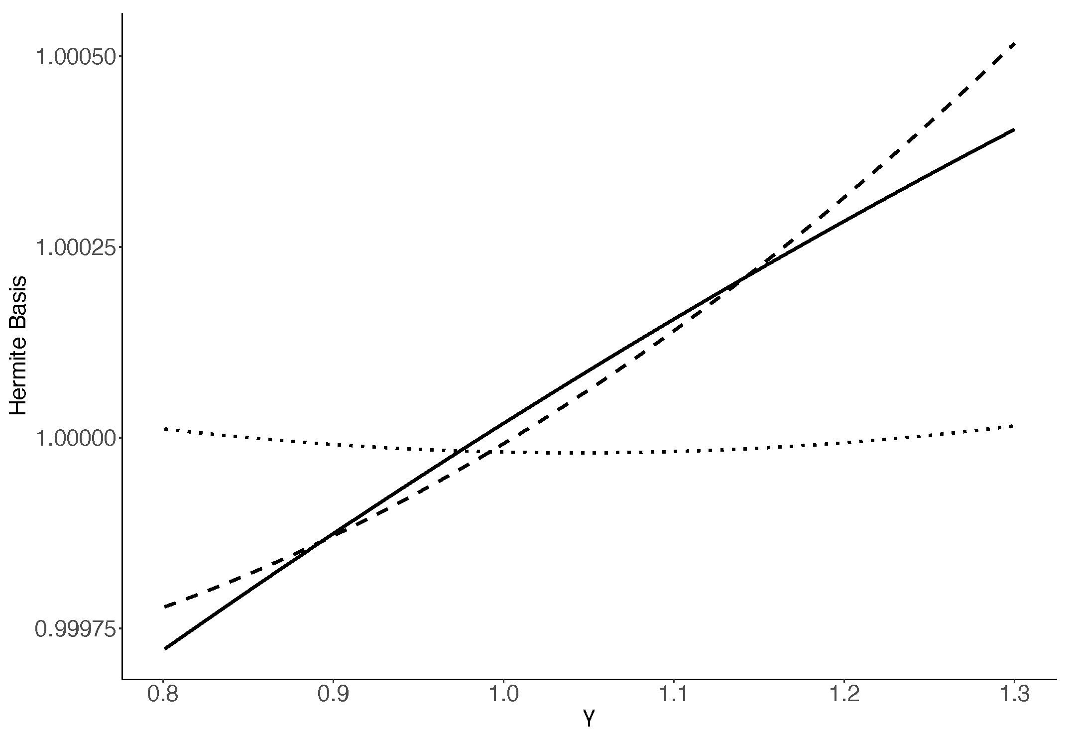
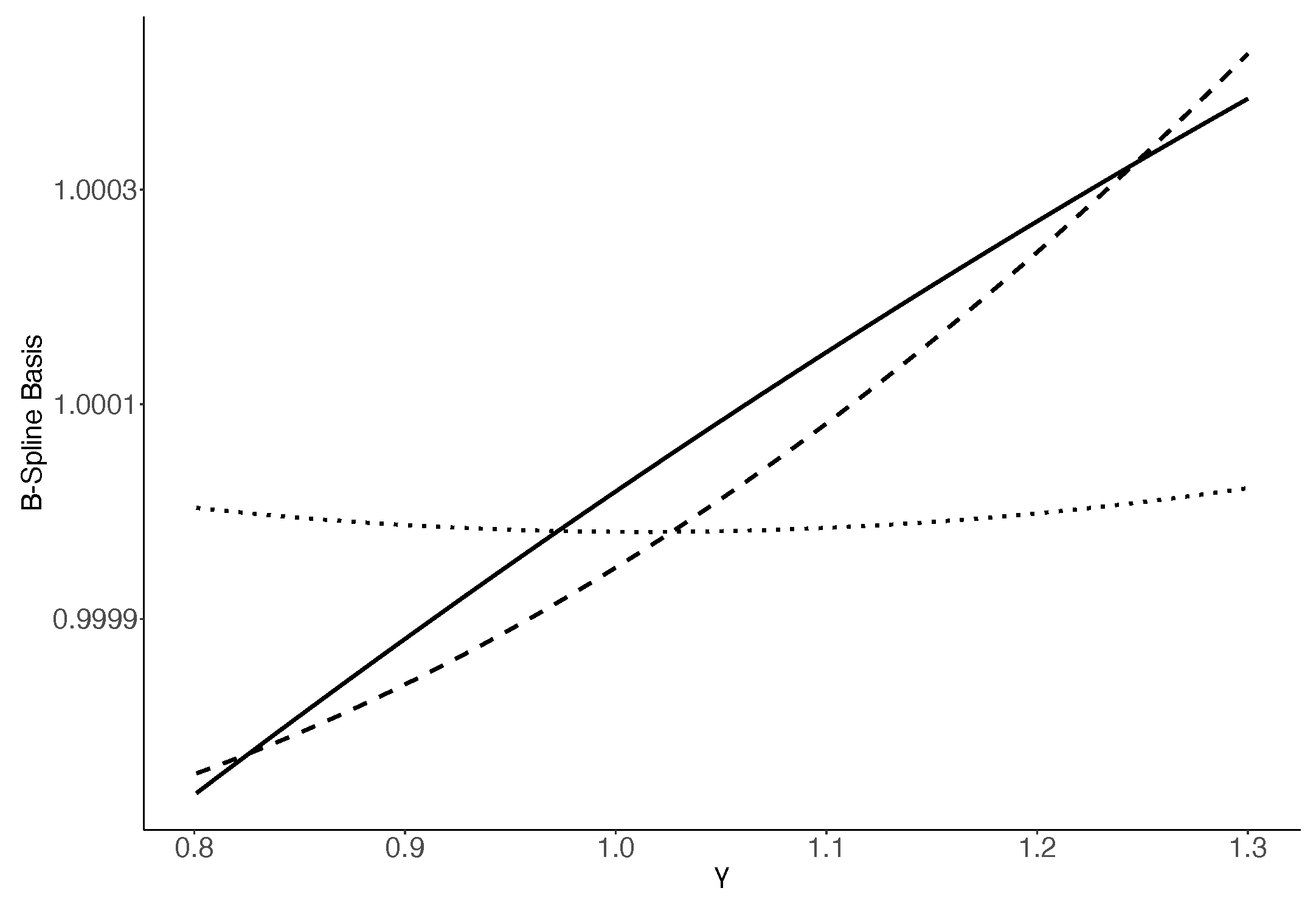
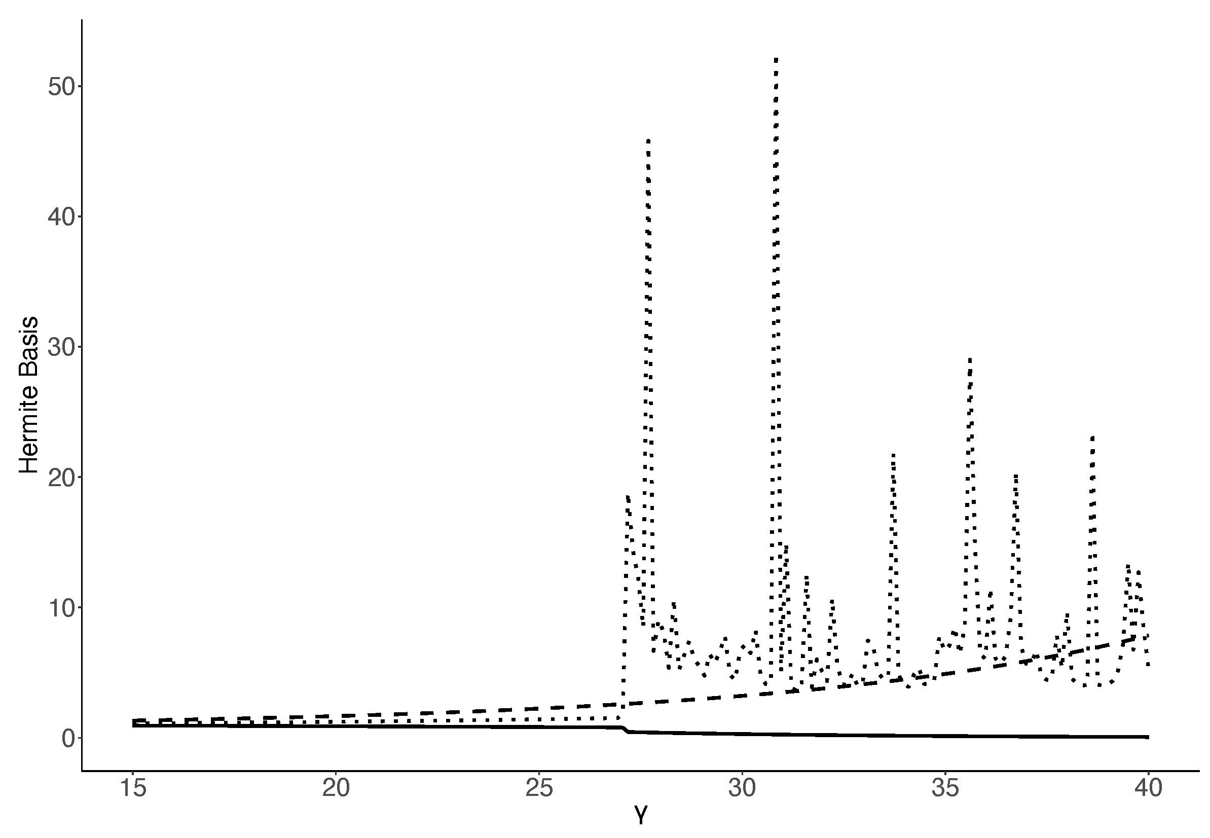
2.2.2. Sieve Estimation Setup

Following Christensen [4] sieve estimation, the infinite-dimensional eigenfunction problem can be solved by a low-dimensional matrix eigenvector problem. Firstly, choose a dictionary of linearly independent basis functions (e.g., hermits, splines, or polynomials) denoted as $b_{k1},\dots ,b_{kk}\in L^2$. Then, there will be a linear subspace spanned by this dictionary $B_k\subset L^2$. One can choose an appropriate dimension k to set up the dictionary. According to Christensen [4]’s study, k will increase when the sample size increases.

To set up the estimation fundamental, let ${\Pi }_k:L^2\to B_k$ be the orthogonal projection onto $B_k$. The eigenfunction problem can be rewritten as follows after a projecting process:

$$\left({\Pi }_{k}M\right){\varphi }_k={\rho }_k{\varphi }_k,$$

(5)

where ${\rho }_k$ is the spectral radius of ${\Pi }_k\mathbb{M}$ and ${\varphi }_k:=\mathcal{X}\to R$ is the correspondent eigenfunction.

The estimation of $\rho ,\varphi$, and ${\varphi }^{*}$ can be approached by solving the following problem:

$${\widehat{\mathbf{M}}}_k{\widehat{c}}_k={\widehat{\rho }}_k\widehat{\mathbf{G}}{\widehat{c}}_k,{\widehat{c}}_k^{{*}^{\prime }}{\widehat{\mathbf{M}}}_k={\widehat{\rho }}_k{\widehat{c}}_k^{{*}^{\prime }}{\widehat{\mathbf{G}}}_k,$$

(6)

where $\widehat{{\rho }_k}$ is the spectral radius of the matrix pair $({\widehat{\mathbf{M}}}_k,{\widehat{\mathbf{G}}}_k)$. ${\widehat{\mathbf{G}}}_k$ and ${\widehat{\mathbf{M}}}_k$ are defined as follows:

$$\widehat{\mathbf{G}}={\displaystyle \frac{1}{n}}\sum _{t=0}^{n-1}{b}^k\left(X_t\right)b^k{\left(X_t\right)}^{\prime };$$

(7)

$$\widehat{\mathbf{M}}={\displaystyle \frac{1}{n}}\sum _{t=0}^{n-1}{b}^k\left(X_t\right)m(X_t,X_{t+1})b^k{\left(X_{t+1}\right)}^{\prime }.$$

(8)

$({\widehat{\rho }}_k,{\widehat{c}}_k,{\widehat{c}}_k^{*})$ can be computed simultaneously using the $qz.dggev$ function in R. Using the values of $({\widehat{c}}_k$,${\widehat{c}}_k^{*})$, $\widehat{\varphi }$ and ${\widehat{\varphi }}^{*}$ can be estimated as:

$$\widehat{\varphi }\left(x\right)=b^k{\left(x\right)}^{\prime }{\widehat{c}}_k,{\widehat{\varphi }}^{*}\left(x\right)=b^k{\left(x\right)}^{\prime }{\widehat{c}}_k^{*},$$

(9)

where $\widehat{{\rho }_k}$ is the spectral radius, ${\widehat{c}}_k$ is its right eigenvector, and ${\widehat{c}}_k^{*}$ is its left eigenvector.

The next step is to derive a solvable formula from the value function expression. Epstein and Zin [1] propose the recursive utility formula to break the connection between the risk-averse parameter and the EIS. Hansen et al. [33] further derive the value function formula by scaling $V\left(X_t\right)$ with $V_t/C_t$:

$$V\left(X_t\right)={\left\{(1-\beta )+\beta \mathbb{E}{[{\left(V\left(X_{t+1}\right)G_{t+1}\right)}^{1-\gamma }\mid X_t]}^{{\displaystyle \frac{1-\theta }{1-\gamma }}}\right\}}^{{\displaystyle \frac{1}{1-\theta }}}.$$

(10)

where $G_{t+1}$ is the per capita consumption growth rate. In this chapter, I use $G_{t+1}=c_{t+1}/c_t$ and $D_{t+1}={\zeta }_{t+1}/{\zeta }_t$ as measurable functions for $(X_t,X_{t+1})$; $X_t=g_t$ or $X_t=(g_t,d_t)$, where $g_t=lg\left(G_t\right)$ and $d_t=lg\left(D_t\right)$.

When the EIS $=1$, (10) can be rewritten as

$$v\left(X_t\right)={\displaystyle \frac{\beta }{1-\gamma }}log\mathbb{E}\left[e^{(1-\gamma )(v\left(X_{t+1}\right)+log{G}_{t+1})}\mid X_t\right],$$

(11)

where $v\left(x\right)=logV\left(x\right)$. The value function and conditional expectation are determined by X.

Using the same reformulation for the recursive problem, the SDF representation can be rewritten as

$$\begin{array}{cc}\hfill {\displaystyle \frac{M_{t+1}}{M_t}}& =\beta G_{t+1}^{-1}{\displaystyle \frac{{\left(V_{t+1}\right)}^{1-\gamma }}{\mathbb{E}\left[{\left(V_{t+1}\right)}^{1-\gamma }\right|X_t]}}\hfill \\ \hfill & =\beta G_{t+1}^{-1}{\displaystyle \frac{{\left(h\left(X_{t+1}\right)\right)}^{\beta }}{\mathbb{T}h\left(X_t\right)}}={\displaystyle \frac{\beta }{\lambda }}{G}_{t+1}^{-\gamma }{\displaystyle \frac{{\left(\chi \left(X_{t+1}\right)\right)}^{\beta }}{\chi \left(X_t\right)}}.\hfill \end{array}$$

(12)

where $h\left(x\right)=e^{{\displaystyle \frac{1-\gamma }{\beta }}v\left(x\right)}$ and the fixed point equation $\mathbb{T}h=h$ come from the Perron–Frobenius problem in Christensen [4]. After these transformation steps, the SDF can be estimated using $\widehat{\chi }$ and $\widehat{\lambda }$. $\widehat{h}\left(x\right)$, $\widehat{\chi }\left(x\right)$, and $\widehat{\lambda }$ can be found by an iteration process. Set $z_1={\widehat{\mathbf{G}}}^{-1}\left({\displaystyle \frac{1}{n}}{\sum }_{t=0}^{n-1}{b}^k\left(X_t\right)\right)$ and apply the iteration method to find $(\widehat{a},\widehat{z})$ with the following conditions (stop iterating when $(a_k,z_k)$ converges to $(\widehat{a},\widehat{z})$):

$$a_k={\displaystyle \frac{z_k}{{\left(z_k^{\prime }\widehat{\mathbf{G}}{z}_k\right)}^{1/2}}},z_{k+1}={\widehat{\mathbf{G}}}^{-1}\mathbf{T}{a}_k.$$

(13)

With $(\widehat{a},\widehat{z})$, $\widehat{h}\left(x\right)$, $\widehat{\chi }\left(x\right)$, and $\widehat{\lambda }$ are obtained as follows:

$$\widehat{h}\left(x\right)={\widehat{\lambda }}^{{\displaystyle \frac{1}{1-\beta }}}{b}^k{\left(x\right)}^{\prime }\widehat{a},\widehat{\chi }\left(x\right)=b^k{\left(x\right)}^{\prime }\widehat{a},\widehat{\lambda }={\left({\widehat{z}}^{\prime }\widehat{\mathbf{G}}\widehat{z}\right)}^{1/2}.$$

(14)

(12) can be reformulated as

$$m(X_t,X_{t+1};(\beta ,\gamma ,{\widehat{\lambda }}_{(\beta ,\gamma )},{\widehat{\chi }}_{(\beta ,\gamma )}))={\displaystyle \frac{\beta }{{\widehat{\lambda }}_{(\beta ,\gamma )}}}{G}_{t+1}^{-\gamma }{\displaystyle \frac{{\left({\widehat{\chi }}_{(\beta ,\gamma )}\left(X_{t+1}\right)\right)}^{\beta }}{{\widehat{\chi }}_{(\beta ,\gamma )}\left(X_t\right)}}.$$

(15)

Then, put the reformulated SDF back to the pricing kernel condition, and the residuals will be expressed as

$$m(X_t,X_{t+1};(\beta ,\gamma ,{\widehat{\lambda }}_{(\beta ,\gamma )},{\widehat{\chi }}_{(\beta ,\gamma )})){\mathbf{R}}_{t+1}-\mathbf{1},$$

where ${\mathbf{R}}_{t+1}$ is the return on asset. The following criterion function is

$$L_n(\beta ,\gamma )={\displaystyle \frac{1}{n}}\sum _{t=0}^{n-1}{\parallel l_n(X_t,\beta ,\gamma )\parallel }^2,$$

(16)

where

$$l_n(x,\beta ,\gamma )=\left({\displaystyle \frac{1}{n}}\sum _{t=0}^{n-1}\left(m(X_t,X_{t+1};(\beta ,\gamma ,{\widehat{\lambda }}_{(\beta ,\gamma )},{\widehat{\chi }}_{(\beta ,\gamma )})){\mathbf{R}}_{t+1}-\mathbf{1}\right)b^k{\left(X_t\right)}^{\prime }\right){\widehat{\mathbf{G}}}^{-1}{b}^k\left(x\right).$$

From (16), we can find that the estimation criterion does not incorporate EIS because the sieve estimation asset pricing model is derived under the maintained assumption of a unit EIS. But empirical evidence indicates that the elasticity of intertemporal substitution (EIS) rarely equals one. This raises an important question: How robust is the sieve asset-pricing model when the EIS deviates from unity? The following section presents a data-generating framework for simulating asset-return series under a non-unit EIS specification to evaluate the model’s robustness and assess the effects of preference misspecification.

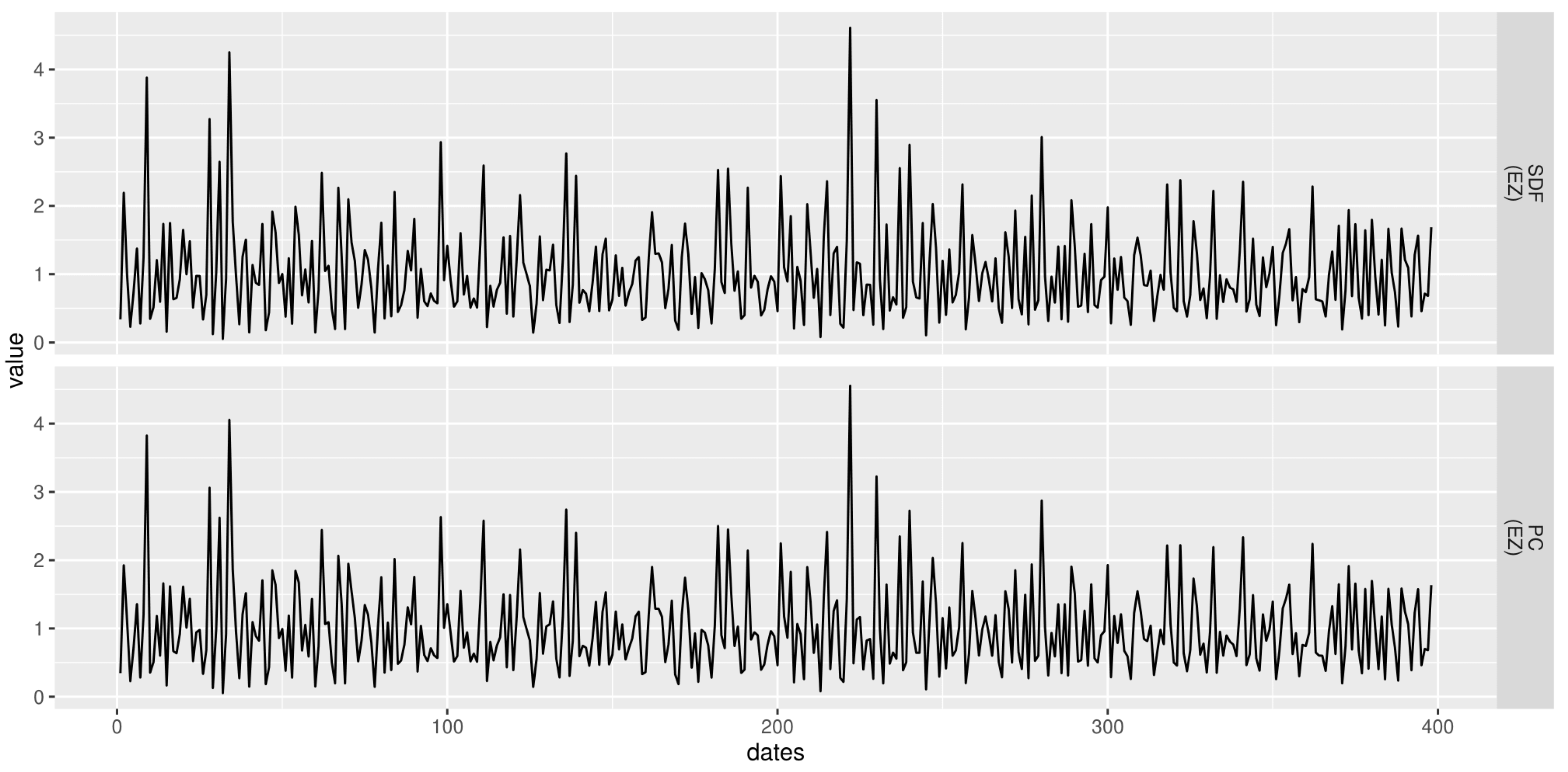
2.2.3. Data-Generating Process

In a consumption-based CAMP model, I draw T observations of consumption growth rates and asset returns by a data-generating process following the method proposed in Tauchen and Hussey [5] and Smith [6]. Smith [6] develops a simulated economy that uses real consumption and dividend series and, under alternative Epstein–Zin preference specifications, generates the corresponding asset returns. By adopting this data-generating framework, I can construct asset-return datasets for a range of preference-parameter configurations.

Following the approximation method in Tauchen and Hussey [5], I construct the consumption and dividend growth rates DGP using finite-state Markov chains. To start this process, I first determine the real aggregate dividend growth and real per capita consumption growth. Tauchen and Hussey [5] calibrate a Markov process to mimic a continuous VAR on those two growth variables. The proposed approximation is set to match the estimate of the log of the annual per capita, real non-durable consumption growth ($g_t=lg(c_t/c_{t-1}$)), the log of the annual S&P 500 aggregate, and real dividend growth ($d_t=lg({\zeta }_t/{\zeta }_{t-1}$)) during the period 1888–1978, which follows a VAR(2) process:

$$\begin{array}{c}\hfill d_t=0.004+0.117d_{t-1}+0.414g_{t-1}+{ϵ}_t^1,\\ \hfill g_t=0.021+0.017d_{t-1}-0.161g_{t-1}+{ϵ}_t^2,\\ \hfill var\left(ϵ\right)=\left[\begin{array}{cc}0.01400& 0.00177\\ 0.00177& 0.00120\end{array}\right],\end{array}$$

(17)

where the Markov approximation is assumed to have jointly normally distributed errors $ϵ=({ϵ}_t^1,{ϵ}_t^2)$ with a covariance matrix as given by $var\left(ϵ\right)$. The parameters of this VAR(2) process are from Kocherlakota [34] using the data from Mehra and Prescott [24].

The Tauchen and Hussey [5] approximation provides a vector of $G_j$($g_j=lg\left(G_j\right)$) and $D_j$($d_j=lg\left(D_j\right)$), $j=1,2,\dots ,S$; a vector of stationary probabilities ${\Pi }_i$, $i=1,2,\dots ,S$; and a set of probability weights ${\pi }_{ij}=Pr\{s_{t+1}=G_j,D_j\mid s_t=G_i,D_i\}$, $i,j=1,2,\dots ,S$. Use $x_{w,t}={\zeta }_{w,t}/{\zeta }_{w,t-1}=G_t$ to denote the growth rate in a dividend paid on the aggregate wealth portfolio and $v_{w,t}=p_{w,t}/{\zeta }_{w,t}$ to denote the price–dividend ratio from the claim on aggregate wealth. Assume S to be the set of all the states and $s_t$ to be the tth state drawn from S. Combining the Euler equation and the simulation design for $R_w$, $R_{sp}$, and $R_f$, which indicate separately the return on a claim whose dividend equals per capita consumption, a claim on the S&P 500 dividend stream, and a claim paying a unit of consumption for sure one period forward, is as follows:

$${\tilde{m}}_{t+1}={\left(\beta {\left({\displaystyle \frac{{\tilde{c}}_{t+1}}{c_t}}\right)}^{-\theta }\right)}^{(1-\gamma )/(1-\theta )}{\tilde{R}}_{w,t+1}^{(1-\gamma )/(1-\theta )-1}.$$

(18)

S equations of $v_{w,i}$ and $v_{w,j}$ can be set up in the following form:

$$v_{w,i}^{(1-\gamma )/(1-\theta )}=\sum _{j=1}^S{\pi }_{ij}\left[{\beta }^{(1-\gamma )/(1-\theta )}{G}_j^{1-\gamma }{(1+v_{w,j})}^{(1-\gamma )/(1-\theta )}\right].$$

(19)

A solution to this system is indicated as $v_w^{*}$, whose value will change corresponding to different values of $\beta$, $\gamma$, and $\theta$. Given a chosen bundle of $\beta$, $\gamma$, and $\theta$, the state returns can be obtained from $v_w^{*}$. Firstly, the return on aggregate wealth over states i and j is given by

$$R_{w,ij}={\displaystyle \frac{1+v_{w,j}^{*}}{v_{w,i}^{*}}}{G}_j.$$

(20)

For a bond paying unity for sure next period, the price in state i is

$${\displaystyle \frac{1}{R_{fi}}}={\beta }^{(1-\gamma )/(1-\theta )}\sum _{j=1}^S{\pi }_{ij}{G}_j^{-\gamma }{\left({\displaystyle \frac{1+v_{w,j}^{*}}{v_{w,i}^{*}}}\right)}^{(\theta -\gamma )/(1-\theta )}.$$

(21)

For the S&P 500 dividend stream, I use a similar system of equations as for the aggregate wealth portfolio, which provides S equations as follows:

$$v_{sp,i}^{(1-\gamma )/(1-\theta )}=\sum _{j=1}^S{\pi }_{ij}\left[{\beta }^{(1-\gamma )/(1-\theta )}{D}_j^{1-\gamma }{(1+v_{w,j})}^{(1-\gamma )/(1-\theta )}\right].$$

(22)

The solution to this equation system is indicated as $v_{sp}^{*}$, and the correspondent state returns are given by

$$R_{sp,ij}={\displaystyle \frac{1+v_{sp,j}^{*}}{v_{sp,i}^{*}}}{D}_j,$$

(23)

where $v_{sp,i}^{*}$ represents the price–dividend ratio of the S&P 500 index in state i. Then, with a random draw of observations, the time series asset return data can be generated according to the state returns.

The next step is to initialize the discount factor $\beta$, relative risk aversion $\gamma$, and intertemporal substitution rate $1/\theta$ to generate simulated asset returns, $R_w$, $R_{sp}$, and $R_f$. I consider several bundles of preference parameters. Guided by the empirical estimates reviewed in Section 2.1.2, I focus on values that are either empirically plausible or deliberately extreme for robustness checks. Specifically, the coefficient of relative risk aversion, $\gamma$, takes the values $0.8$, $5.2$, and 25. The EIS, $\theta$, is set to $0.8$, $5.2$, and 29. I label the bundle $\beta =0.985$ and $(\gamma ,\theta )=(0.8,0.8)$ the plausible bundle, as this combination is well supported by the empirical evidence. To study performance under extreme conditions and to relate to the equity premium puzzle literature, I also examine the settings $(\gamma ,\theta )=(25,29)$ and $(\gamma ,\theta )=(5.2,5.2)$, parameterizations considered by Kandel and Stambaugh [35], Kocherlakota [34], and Christensen [4].

3. Results

3.1. Study with the Generated Dividend and Consumption Growth Rates

In this part, I use the generated data of consumption and dividend growth rates and asset returns to estimate important parameters and change of measure using the sieve asset pricing model. The summarized statistics for consumption and dividend growth rates are shown in

Table 1. Summary of Consumption and Dividend Growth. Mean and standard error estimates from the generated consumption and dividend growth using 500 draws of 400 annual observations.

			Estimates
Variable		Intercept	${\mathit{d}}_{\mathit{t}-\mathbf{1}}$	${\mathit{g}}_{\mathit{t}-\mathbf{1}}$	Var ($ϵ$)	Cov ($ϵ$)
dt	Mean Point Estimate	0.004	0.111	0.416	0.014	0.002
	Standard Error	0.007	0.054	0.186
gt	Mean Point Estimate	0.021	0.017	−0.161	0.001	0.002
	Standard Error	0.002	0.016	0.054

. It lists the information of the Monte Carlo simulation using 500 draws of 400 observations from an annual data-generating process. The dividend growth rate and consumption growth rate are generated following the DGP discussed in Section 2.2.3. The represented mean estimate, variance, and covariance are listed. The Mean Point Estimate of the intercept is close to the population values in (17). The number values in the variance–covariance matrix are close to the ones in the population. The estimated coefficients for dividend and consumption growth rates are also close to their population values. By setting up different values of $\beta$, $\theta$, and $\gamma$ and using the consumption and dividend growth rate data, I can generate multiple economies which can give us different asset pricing data. The summarized statistics of asset returns and the mean equity premium $(R_{sp}-R_f)$ in Monte Carlo simulation are shown in

Table 2. Summary of Asset Returns.

$\mathit{\gamma }$, $\mathit{\theta }$		${\mathit{R}}_{\mathit{w}}$	${\mathit{R}}_{\mathit{s}\mathit{p}}$	${\mathit{R}}_{\mathit{f}}$	Equity Premium
0.8, 0.8	Mean of estimates	0.036	0.038	0.035	0.003
	Std. dev. Of estimates	0.035	0.125	0.004
5.2, 5.2	Mean of estimates	0.114	0.116	0.104	0.012
	Std. dev. Of estimates	0.063	0.136	0.030
25, 29	Mean of estimates	0.268	0.265	0.137	0.128
	Std. dev. Of estimates	0.254	0.262	0.170

. From the replicated data-generating process, the mean estimates of asset returns are increasing when either $\theta$ or $\gamma$ increases. This increasing trend is consistent with Smith [6], while the equity premium is smaller than or close to $0.01$ when $\theta$ and $\gamma$ are small. This result is consistent with Weil [25]. When $(\gamma ,\theta )$ takes the extreme value $(25,29)$, the equity premium is larger than $0.01$. The standard deviations of asset returns with different pairs of $(\gamma ,\theta )$ values are close to Smith [6].

First, we revisit the key decomposition estimation in Christensen [4] using the extreme parameter bundle $(\gamma ,\theta )=(25,29)$ and the estimated left eigenfunction is represented in Figure A1. k is chosen to be eight to coincide the same value of k in Christensen [4] for a similar sample size. $\widehat{\varphi }$ given $g_t$ is shown as an upward curve within a proper range, which is following the fact that the transitory component of the SDF is suggested to be very small. $\widehat{\varphi }$ given $(g_t,d_t)$ is also upward sloping in the middle part of the domain for $g_t$ and $d_t$. Figure A2 shows that the estimated right eigenfunction ${\widehat{\varphi }}^{*}$ has a downward sloping trend which is different from what theories suggest. From what the contour plot shows, the downward sloping trend is evident when $d_t$ and $g_t$ are both small, and when $d_t$ is small and $g_t$ is large. Figure A3 shows the estimated change of measure ($\widehat{\varphi }{\widehat{\varphi }}^{*}\left(x\right)$), which is the Nikodym derivative of $\tilde{Q}$ with respect to Q. $\widehat{\varphi }$ is upward sloping and relatively flat while ${\widehat{\varphi }}^{*}\left(x\right)$ is downward sloping. Therefore, the estimated change of measure is downward sloping based on $x_t$. Given $(g_t,d_t)$, it is estimated to be downward sloping when $d_t$ and $g_t$ are both small, and when $d_t$ is small, $g_t$ is large. All those estimation results closely align with the benchmark model in Christensen [4].

Figure 1 presents the SDF and its permanent component under the recursive utility setup. When the EIS is not one, the estimated permanent component follows the martingale property and is relatively larger than the transitory one. This result indicates that if the permanent component has been ignored then the estimation can hardly be identifiable. The robustness results for the parameter bundles $(\gamma ,\theta )=(0.8,0.8)$ and $(\gamma ,\theta )=(5.2,5.2)$ are reported in

Table A1. Estimates of $\rho ,y$, and $L,$ when $\beta =0.985,\theta =0.8,$ and $\gamma =0.8$.

	${\mathit{X}}_{\mathit{t}}={\mathit{g}}_{\mathit{t}}$	${\mathit{X}}_{\mathit{t}}=({\mathit{g}}_{\mathit{t}},{\mathit{d}}_{\mathit{t}})$	${\mathit{X}}_{\mathit{t}}=({\mathit{g}}_{\mathit{t}},{\mathit{d}}_{\mathit{t}})$
$\widehat{\rho }$	0.9616	0.9633	0.9888	0.9888	0.9889
	(0.9533, 0.9667)	(0.9562, 0.9706)	(0.9876, 0.9898)	(0.9876, 0.9899)	(0.9877, 0.9899)
$\widehat{y}$	0.0391	0.0374	0.0113	0.0112	0.0112
	(0.0339, 0.0477)	(0.0298, 0.0447)	(0.0102, 0.0125)	(0.0102, 0.0125)	(0.0101, 0.0124)
$\widehat{L}$	0.4039	0.1316	0.0002	0.0003	0.0003
	(0.1640, 0.7158)	(−0.1750, 0.1724)	(0.0002, 0.0003)	(0.0002, 0.0003)	(0.0002, 0.0004)
$\widehat{\beta }$	0.9375	0.9492	0.99	0.99	0.99
	(0.9208, 0.9513)	(0.9429, 0.9700)
$\widehat{\gamma }$	33.7604	19.119	0.7	0.8	0.9
	(31.3992, 53.6258)	(8.2750, 24.6641)
$\widehat{\lambda }$	1.426	1.1010	1.0004	1.0002	1.0001
	(1.0347, 1.7873)	(0.7365, 1.1395)	(1.0000, 1.0007)	(1.0001, 1.0005)	(1.0000, 1.0003)

and

Table A2. Estimates of $\rho ,y$, and $L,$ when $\beta =0.985,\theta =5.2$, and $\gamma =5.2$.

	${\mathit{X}}_{\mathit{t}}={\mathit{g}}_{\mathit{t}}$	${\mathit{X}}_{\mathit{t}}=({\mathit{g}}_{\mathit{t}},{\mathit{d}}_{\mathit{t}})$	${\mathit{X}}_{\mathit{t}}=({\mathit{g}}_{\mathit{t}},{\mathit{d}}_{\mathit{t}})$
$\widehat{\rho }$	0.8944	0.8974	0.9912	0.9919	0.9926
	(0.8877, 0.8972)	(0.8928, 0.9021)	(0.9876, 0.9898)	(0.9896, 0.9922)	(0.9900,0.9928)
$\widehat{y}$	0.1116	0.1082	0.0089	0.0081	0.0074
	(0.1085, 0.1190)	(0.1030, 0.1134)	(0.0084, 0.0109)	(0.0078, 0.0104)	(0.0072,0.0100)
$\widehat{L}$	0.154	0.0999	0.0058	0.0091	0.0132
	(−0.0449, 0.2820)	(0.0935, 0.1931)	(0.0030, 0.0050)	(0.0047, 0.0078)	(0.0068,0.0112)
$\widehat{\beta }$	0.8804	0.8857	0.99	0.99	0.99
	(0.8652, 0.8934)	(0.8725, 0.8991)
$\widehat{\gamma }$	19.1893	15.8118	4	5	6
	(13.0482, 31.2515)	(8.3206, 27.8645)
$\widehat{\lambda }$	1.1376	1.0797	0.9993	1.0005	1.0025
	(0.9030, 1.2622)	(0.8705, 1.1592)	(1.0000, 1.0007)	(0.9936, 1.0034)	(0.9934,1.0057)

, respectively, and attest to the model’s stability across different preference specifications

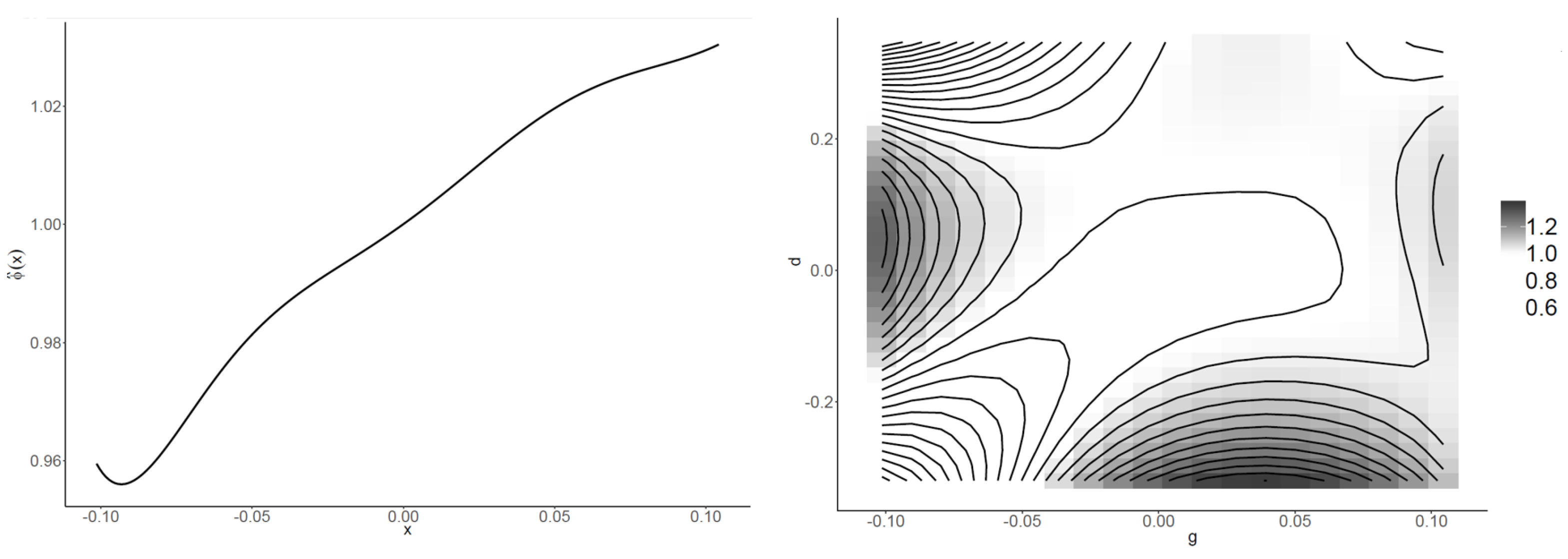
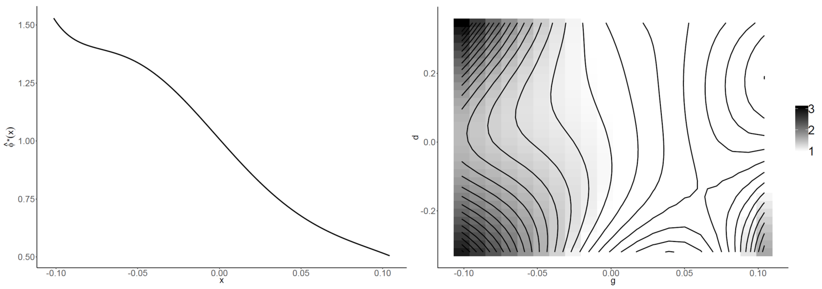
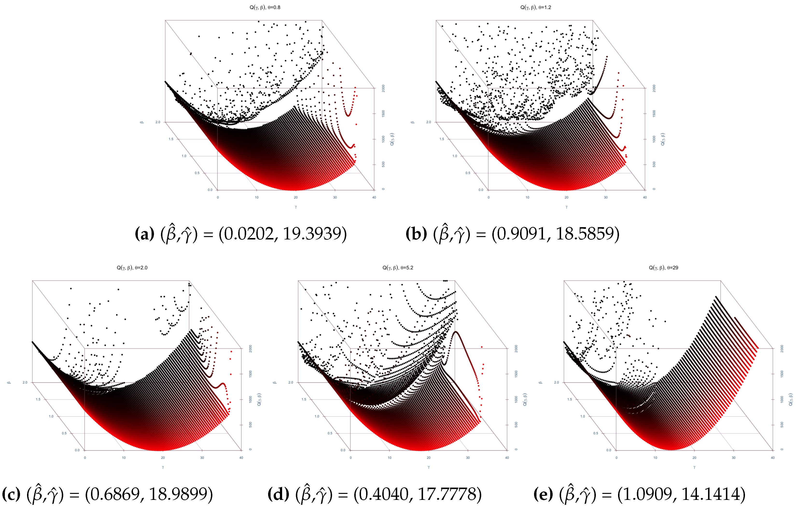
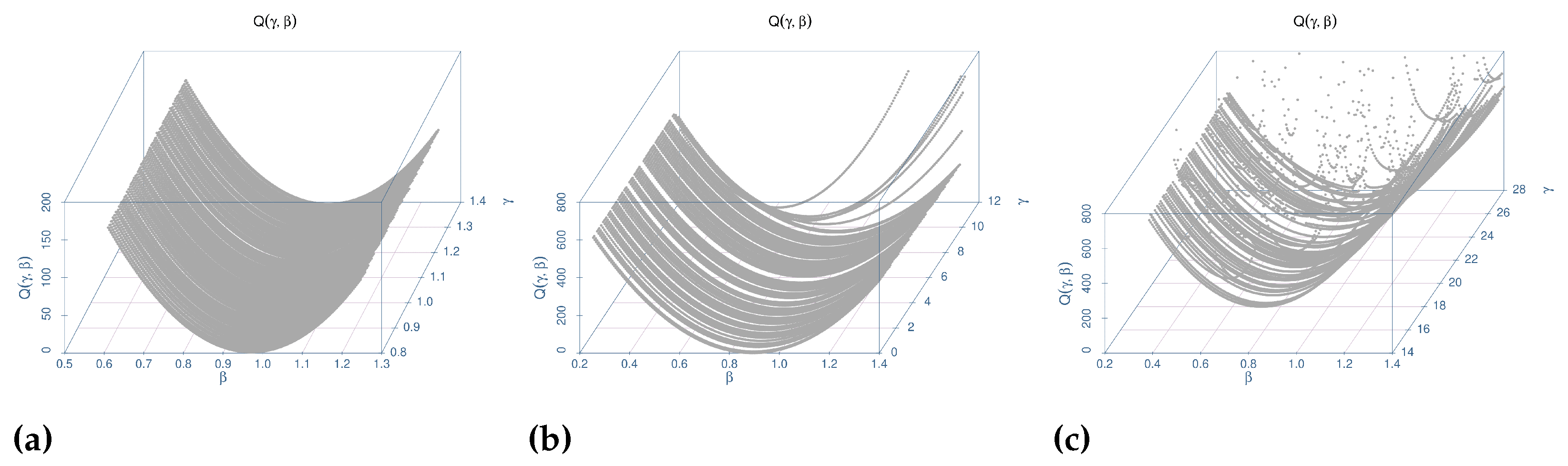
3.2. Estimation Surface Study

In this part, I study the surface of the objective function for sieve estimation to show the performance of the sieve asset pricing model for non-unit EIS cases. Keeping $\beta =0.985$ and $\gamma =0.8$, letting $\theta$ choose non-unit values $0.8$, $1.2$, 2, $5.2$, and 29, I generate different economies’ asset return data according to each bundle of parameters. For each generated economy, compute the value of $Q_{(\gamma ,\beta )}$ and draw the objective function. The objective function is defined as:

$$Q(\beta ,\gamma )=\left({\displaystyle \frac{1}{n}}\sum _{t=0}^{n-1}\left(m(X_t,X_{t+1};(\beta ,\gamma ,\theta ,{\lambda }_{(\beta ,\gamma ,\theta )},{\chi }_{(\beta ,\gamma ,\theta )})){\mathbf{R}}_{t+1}-\mathbf{1}\right)b^k{\left(X_t\right)}^{\prime }\right){\widehat{\mathbf{G}}}^{-1}{b}^k\left(x\right),$$

(24)

where $X_t=g_t$, $t=1,2,\dots ,400$.

Figure 2 shows the estimation surface for $\widehat{\gamma }$ and $\widehat{\beta }$ across different economies corresponding to different bundles of parameters. Panels (a–c) depict the estimation surface for plausible EIS values, while panels (d,e) illustrate the surface for more extreme EIS values. For plausible values of parameters, the estimation surfaces are concave and stable. Model stability deteriorates as $\theta$ becomes increasingly extreme, yet the surface retains its concave shape even at very high $\theta$. This result supports the overall robustness of [4]’s work. Although the true risk-aversion parameter is $\gamma =0.8$, the estimates cluster around $\widehat{\gamma }\approx 20$, indicating a substantial upward bias. The comparison plots also reveal a systematic shift when only the EIS input changes while $\gamma$ and $\beta$ are held constant: when the true value of the EIS increases, the estimated $\gamma$ declines noticeably. This key robustness result indicates that, under the model’s unit EIS restriction, data that actually contain signals of a high EIS lead to distorted estimates, with the information that should be attributed to the EIS instead being absorbed by the risk-aversion parameter and time discount factor. Additionally, the distortion in $\gamma$ is monotonic because of the intuitive relationship between $\gamma$ and $EIS$, and the distorted $\gamma$ estimations show a monotone trend: the farther the true EIS departs from unity, the more of its signal is absorbed by $\gamma$, widening the gap between the estimated $\widehat{\gamma }$ and the baseline value of roughly 20. Noticeably, this trend is also observed in experiments with large $\gamma$ values when all other parameters are held as in the previous experiment. The estimation surface for $\beta$ is concave and relatively flat, remaining stable for plausible EIS values. However, it becomes unstable as the EIS increases beyond that range.

To reinforce the robustness analysis, I expand the study to a denser grid of parameter values. The previous experiment examined only five discrete bundles, but the next step varies each parameter in small increments across a wider range. Figure 3 presents the surface for $\widehat{\beta }$ when $\gamma$ is fixed at its data-generating value. The surface is plotted for $\theta =0.8,5.2$, and 29, with $\gamma$ taking 100 evenly spaced values within the intervals $[0.8,1.4]$, $[0,12]$, and $[14,28]$, respectively. Each value of $\gamma$ in these intervals defines a distinct parameter bundle for generating the asset-return data, and each curve in the figure shows the objective function as $\beta$ varies with $\gamma$ held at its data-generating value. In most cases, the surface remains concave, attaining its minimum close to the true $\beta$. Instability becomes apparent only when $\gamma$ exceeds approximately 9.5. Relative to the surfaces obtained for $\widehat{\gamma }$, the estimation of $\widehat{\beta }$ exhibits greater robustness, evidenced by consistently stable concavity and markedly smaller bias.

The procedure for constructing the estimation surface for $\widehat{\gamma }$ mirrors that for $\widehat{\beta }$, except that $\beta$ is varied while $\gamma$ separate surface line is plotted. Let $\beta$ take 100 grid points in the intervals $[0.7,1.4]$, $[0.2,1.4]$, and $[0.7,1.4]$, corresponding to $(\gamma ,\theta )$ bundles of $(0.8,0.8)$, $(5.2,5.2)$, and $(25,29)$, respectively. For each $(\gamma ,\theta )$ bundle, $\beta$ is first varied over a 100-point grid, and for each $\beta$ the objective function is calculated as $\gamma$ moves across 100 grid points within its designated interval. The $\gamma$ intervals $(0,2)$, $(0,12)$, and $(15,40)$ align with the corresponding $\theta$ values. The separate surface plot for $\widehat{\gamma }$ is shown in Figure 4. Unlike the estimation surface for $\widehat{\beta }$, the surface for $\widehat{\gamma }$ is non-concave and increases with $\gamma$ in the lower range. Because of this non-concavity, the optimization routine is highly sensitive to its initial starting value. Consequently, the algorithm often converges to a local, rather than global, minimum for $\widehat{\gamma }$. This feature explains why the bias of $\widehat{\gamma }$ diminishes as the true $\gamma$ approaches the initial value. This instability helps explain why Christensen [4] consistently receives extremely large estimates of $\widehat{\gamma }$.

To investigate why the estimation of $\widehat{\gamma }$ lacks robustness, I decompose the objective function and examine each component, looking for insights that may generalize to a wider class of asset pricing models. I begin by recalling the formula for the generalized residuals:

$$m(X_t,X_{t+1};(\beta ,\gamma ,\theta ,{\widehat{\lambda }}_{(\beta ,\gamma ,\theta )},{\widehat{\chi }}_{(\beta ,\gamma ,\theta )})){\mathbf{R}}_{t+1}-\mathbf{1},$$

$$m(X_t,X_{t+1};(\beta ,\gamma ,\theta ,{\widehat{\lambda }}_{(\beta ,\gamma ,\theta )},{\widehat{\chi }}_{(\beta ,\gamma ,\theta )}))={\displaystyle \frac{\beta }{{\widehat{\lambda }}_{(\beta ,\gamma ,\theta )}}}{G}_{t+1}^{-\gamma }{\displaystyle \frac{{\left({\widehat{\chi }}_{(\beta ,\gamma ,\theta )}\left(X_{t+1}\right)\right)}^{\beta }}{{\widehat{\chi }}_{(\beta ,\gamma ,\theta )}\left(X_t\right)}}.$$

There are three components in this SDF expression. By allowing $\gamma$ to vary over the range $0.8$ to 10, I trace how each component responds to changes in risk aversio. In Figure 5, I show their values or mean values for both the Hermite and B-Spline Basis function cases, since both $G_t^{-\gamma }$ and ${\displaystyle \frac{{\left({\widehat{\chi }}_{(\beta ,\gamma ,\theta )}\left(X_{t+1}\right)\right)}^{\beta }}{{\widehat{\chi }}_{(\beta ,\gamma ,\theta )}\left(X_t\right)}}$ are vectors. Here, I only show the mean points of all time periods values when $\gamma$ is varying. ${\widehat{\lambda }}_{(\beta ,\gamma )}^{-1}$ is not monotone—first increasing then decreasing. ${\displaystyle \frac{{\left({\widehat{\chi }}_{(\beta ,\gamma ,\theta )}\left(X_{t+1}\right)\right)}^{\beta }}{{\widehat{\chi }}_{(\beta ,\gamma ,\theta )}\left(X_t\right)}}$ and $G_t^{-\gamma }$ both have an upward trend; especially, $G_t^{-\gamma }$ has a dominating increasing trend. This explanation is the main reason why the objective function is particularly sensitive in $\gamma$. Similar results for cases when $(\gamma ,\theta )=(0.8,0.8),(25,29)$ are shown in Figure A4, Figure A5, Figure A6 and Figure A7. Since the $G_t^{-\gamma }$ part is an exponential function and consequentially ${\displaystyle \frac{{\left({\widehat{\chi }}_{(\beta ,\gamma ,\theta )}\left(X_{t+1}\right)\right)}^{\beta }}{{\widehat{\chi }}_{(\beta ,\gamma ,\theta )}\left(X_t\right)}}$ is increasing in $\gamma$ rapidly. It can be concluded that the factor leading to the failure of estimating $\gamma$ is at least in part, from a structural limitation of consumption-based models with the $G_t^{-\gamma }$ term. Using aggregate consumption data already restricts information. This exponential term amplifies even minor measurement errors, thereby exacerbating robustness problems.

4. Discussion

4.1. The Efficiency of the Robustness Framework

I contribute a fresh methodological perspective to asset pricing research. Instead of proposing a new preference specification or an altered economic mechanism, the method scrutinizes a central model for sensitivity and robustness study according to a critical preference parameter assumption. This complements the foundational works of Epstein–Zin and Bansal–Yaron by operating in the reverse direction: rather than altering assumptions to fix model shortcomings, it varies the environment to test the robustness of a cutting-edge estimation method under the original assumptions. The approach questions the trust I can place in the estimated parameters of standard asset pricing models when preferences in reality might differ from what was assumed. This robustness study provides a deeper understanding of the Perron–Frobenius sieve estimation’s reliability in the context of Epstein–Zin type models, all while staying within the framework of the original model. It thereby bridges the gap between classic model-centric innovations and modern estimation techniques, highlighting how a well-established model behaves under subtle shifts in preference parameters without overhauling its core.

4.2. The Insights of Christensen 2017 Robustness Study

The robustness analysis reveals that the Christensen [4] sieve estimation framework remains largely stable in its core inference when the elasticity of intertemporal substitution (EIS) deviates from unity. In this robustness analysis, using a data-generating process with a non-unit EIS, the estimation of the time discount factor ($\beta$) proves robust. The sieve method accurately recovers $\beta$ even as the true EIS departs from one, indicating that the long-run discounting behavior of the model is identified reliably by the available moment conditions. In contrast, the estimation of the risk aversion coefficient ($\gamma$) is markedly more sensitive to EIS misspecification. The deviations in the EIS from unity lead to noticeable shifts or bias in the estimated $\gamma$, reflecting a less stable identification. This divergence underscores a limitation: the model’s ability to pin down agents’ attitude toward risk through $\gamma$ is fragile when intertemporal substitution behavior is not as originally assumed.

Several structural features help explain why the time discount factor is estimated with greater stability than the risk aversion coefficient. The time discount factor mainly influences intertemporal consumption–savings decisions in a way that affects aggregate consumption growth and the level of the risk-free rate. These features of the data remain relatively observable and unaffected even if consumers’ EIS deviates from 1, as long as households still optimize intertemporally. In contrast, the risk aversion parameter governs the curvature of utility and affects how strongly consumers dislike consumption volatility and how large the equity premium is given the consumption process. When the model assumes EIS $=1$, it effectively imposes a specific substitution effect that, if untrue, can distort the inferred relationship between consumption risk and asset returns. In the robustness tests, the model’s fixed structure conflated the effects of risk aversion and intertemporal substitution. For instance, an economy with the EIS $>1$ might produce data that mimic the effects of lower risk aversion from the model’s perspective since consumers appear to smooth consumption less. As Christensen [4] is unable to adjust the EIS, the author may then incorrectly attribute some of that behavior to the risk aversion parameter. This leads to biased risk aversion estimates or a flatter estimation objective surface in the direction of $\gamma$, making it difficult to identify the true value. The objective function surface analysis illustrates that the estimated objective has a well-defined minimum in the $\beta$ dimension, indicating a steep curvature that yields a unique optimum for $\beta$. In the $\gamma$ dimension, however, the surface is comparatively flatter and more irregular when data are generated with higher EIS values. This increased flatness suggests that a range of $\gamma$ values can nearly equally satisfy the Euler equations when the EIS is misspecified, making the true $\gamma$ harder to pinpoint. Such behavior indicates that the data do not provide a strong unique signal for risk aversion once the model’s assumption is misaligned with actual consumer behavior.

4.3. Implications for Broader Asset Pricing Models

The above findings carry important implications for asset pricing models beyond the specific Christensen [4] sieve framework. In empirical asset pricing, it is common to estimate or calibrate model parameters under certain assumptions, and the results highlight what can happen if the true values violate those assumptions. A positive message is that some parameters may be robust to moderate misspecification. This suggests that features like the effective discount rate or long-run growth rate of the stochastic discount factor can be inferred reliably from data even if some preference parameters are misspecified. The experiment indicates that the parameter recovery for time preference is robust and implies that certain fundamental aspects of an asset pricing model are identifiable and trustworthy.

However, my results also indicate a cautionary tale. When a model is estimated on data that are inconsistent with its own assumptions, estimated parameters can become unreliable. The difficulty in recovering the risk aversion coefficient in the robustness test is a stark example of how a seemingly sound estimation can break down if the data violate key model conditions. In a broader sense, this suggests that misspecification in preferences or functional form can lead to a false sense of confidence in estimated parameters. An empirical researcher might estimate a structurally plausible-looking value for risk aversion using a misspecified model, not realizing that the estimate is largely driven by the model’s constraints rather than the data’s true signal. The findings echo the general principle in econometrics that identification requires correct model specification: when the actual data-generating process lies outside the model’s assumed family, some parameters, especially those governing nonlinearities or higher-order moments, may not be identifiable or can only be recovered by pushing them to extreme values.

4.3.1. The Revealed Absorption Effect and Justification

When the Perron–Frobenius sieve estimator fixes the EIS at unity, feeding the model data from an economy with the EIS $\ne 1$ forces the model to attribute any resulting discrepancies from the EIS to risk aversion and time discount factors. I summarize this effect as the “Absorption Effect”, which describes when imposing the unit EIS assumption, the misspecified intertemporal substitution behavior is absorbed by the estimated risk-aversion parameter and time discount factors, distorting their identification. Uncovering this absorption effect is therefore empirically and theoretically important. It highlights that what might appear as evidence of changes in risk aversion or time discount factors may in fact be an artifact of a misspecified EIS.

In particular, when the true EIS differs from unity, an actual EIS deviating from one tends to be offset by an under- or over-estimated coefficient of relative risk aversion in a unit-EIS estimation. Because under a unit-EIS specification, the model must “pretend” that the agent is more or less risk-averse to match observed asset returns. The further the true EIS lies from unity, the more pronounced this distortion becomes. Given this sensitivity, researchers can adopt a preestimation step to know the true values of the EIS to justify their estimates. First, one estimates the EIS using the empirical data without constraining them to one. In the second step, for the unit EIS model, the estimated risk aversion is then interpreted as an upper or lower bound depending on the EIS finding. For instance, if the estimated EIS from the first step is found to be less than one, the unit EIS model estimated risk aversion is likely understated. In sum, the unit-EIS absorption effect means that a misspecified EIS can disguise itself as distorted risk aversion, and recognizing this, analysts first pin down the EIS and then adjust their risk aversion estimates accordingly. By acknowledging the misspecification from the assumption, one avoids attributing all asset pricing puzzles solely to risk aversion. Such context confirms that the often puzzlingly high-risk aversion estimates under unit EIS are largely an artifact of misspecification.

4.3.2. Connection to Asset Pricing Models

Firstly, the findings help explain why the traditional consumption CAPM with log utility (EIS = 1) struggled to jointly match the low risk-free rate and high equity premium without implausible high-risk aversion. The standard CCAPM effectively assumes a unitary link between intertemporal substitution and risk aversion, so a deviation in the true EIS means the model is calibrated or estimated with the wrong curvature. The robustness results caution that in such cases, the risk aversion parameter will adjust in bias-prone ways. If the actual EIS is lower or higher than one, forcing a unit EIS model to fit the data can lead to distorted $\gamma$ estimates, echoing early empirical findings of unstable or divergent parameter estimates in consumption Euler equations. The analysis underscores that models like the CCAPM must be cautious in interpreting recovered preference parameters, as a stable $\beta$ may mask a misspecified $\gamma$ when the EIS assumption is wrong. More importantly, the components analysis reveals that the consumption component constitutes a large share of the objective function, causing the optimization procedure to be heavily influenced by variations in the consumption component. Using aggregated consumption data, an estimation that is disproportionately influenced by the consumption component rarely captures the true underlying signals.

Secondly, this robustness exercise, which effectively operates in an Epstein–Zin-like setting, confirms both the promise and the challenge of such models. The promise is that the discount factor is recoverable even under complex preference configurations, which is a reassuring result for long-horizon pricing kernels. The challenge, however, is that the risk aversion parameter may not be precisely identified even when allowed to vary freely. The results show that it is hard to recover in finite samples when consumption dynamics or instrument information are limited. This outcome aligns with known difficulties in estimating recursive utility models. Empirical studies have produced widely varying estimates of the EIS and risk aversion across different specifications, highlighting near-identification problems in separating the two forces. My study makes this concrete by showing that if the modeler assumes the wrong EIS, the estimated attitude toward risk can shift significantly without devastating the fit. I find that some asset pricing moments can be matched by tweaking $\gamma$ to compensate for a misspecified EIS. This insight adds nuance to the interpretation of Epstein–Zin model estimations: a good model fit does not guarantee that each underlying preference parameter is correctly identified, especially if one of them (the EIS) is miscalibrated.

Thirdly, long-run risk frameworks rely on an extreme EIS in conjunction with significant risk aversion to generate sizable risk premia and volatility in asset prices. In these models, an EIS that departs substantially from unity magnifies the impact of persistent consumption growth shocks on asset valuations, thereby allowing moderate $\gamma$ values to produce a large equity premium. My robustness analysis provides a cautionary perspective: if the true EIS in the data is not as high as assumed, the model’s calibration of $\gamma$ might silently absorb the discrepancy. I find that $\beta$, which in long-run risk calibrations mostly influences the risk-free rate level, would remain identifiable, but an assumed EIS mismatch would make inferred risk aversion less reliable. This is consistent with the mechanics of long-run risk models. A misspecified EIS alters how strongly agents price long-run consumption risks, and the model may require an artificially higher or lower $\gamma$ to fit the observed asset returns in compensation. Thus, the robustness study underscores a key point: preference parameter recovery can be fragile. Though the recursive utility method is powerful, researchers should interpret the estimated parameters with caution.

5. Conclusions

In conclusion, my proposed robustness design is efficient and helps uncover and analyze the nature of preference information and reveal how these preferences may be misspecified. My investigation demonstrates that, on one hand, the core insights of the original study prove replicable under the EIS $\ne 1$: the nonparametric sieve method still identifies a dominant permanent component in the stochastic discount factor, validating the long-run risk decomposition even in alternative preference environments, and is able to explain the spread between equity and bond returns evidenced in my results. These findings attest to the overall robustness of the Christensen’s eigenfunction approach to SDF estimation. On the other hand, my results uncover the robustness in time discount factor recovery and a fragility in risk aversion parameter recovery. The time discount factor is estimated with remarkable stability across different true EIS values, suggesting that discounting over time is captured reliably. In contrast, the risk aversion coefficient is sensitive and prone to misidentification. When the true EIS differs from the model’s unit value, the estimated risk aversion surface changes sharply and tends to become flatter when the EIS is bigger. The risk aversion parameter effectively absorbs the misspecification in EIS preferences. This absorption effect means that a model can mask substantial errors in interpreting risk premia, with the unit EIS assumption causing the model to attribute too much or too little curvature to the utility function. The implications for broader asset pricing models are immediate, and the findings suggest that researchers must be careful about hidden assumption violations. The findings broaden the credibility of Christensen’s framework by charting a path to ensure that long-run risk estimations do not come at the expense of sound economic identification and bridge the gap between elegant theory and reliable empirical application.

References

1. Epstein, L.G.; Zin, S.E. Substitution, Risk Aversion, and the Temporal Behavior of Consumption and Asset Returns: A Theoretical Framework. Econometrica 1989, 57, 937–969. [Google Scholar] [CrossRef]
2. Bansal, R.; Yaron, A. Risks for the Long Run: A Potential Resolution of Asset Pricing Puzzles. J. Financ. 2004, 59, 1481–1509. [Google Scholar] [CrossRef]
3. Hansen, L.P.; Scheinkman, J.A. Long-Term Risk: An Operator Approach. Econometrica 2009, 77, 177–234. [Google Scholar]
4. Christensen, T.M. Nonparametric Stochastic Discount Factor Decomposition. Econometrica 2017, 85, 1501–1536. [Google Scholar] [CrossRef]
5. Tauchen, G.; Hussey, R. Quadrature-Based Methods for Obtaining Approximate Solutions to Nonlinear Asset Pricing Models. Econometrica 1991, 59, 371–396. [Google Scholar] [CrossRef]
6. Smith, D.C. Finite sample properties of tests of the Epstein-Zin asset pricing model. J. Econom. 1999, 93, 113–148. [Google Scholar] [CrossRef]
7. Moskowitz, T.J.; Vissing-Jorgensen, A. The Returns to Entrepreneurial Investment: A Private Equity Premium Puzzle? Am. Econ. Rev. 2002, 92, 745–778. [Google Scholar] [CrossRef]
8. Campbell, J.Y.; Viceira, L.M. Consumption and Portfolio Decisions when Expected Returns are Time Varying. Q. J. Econ. 1999, 114, 433–495. [Google Scholar] [CrossRef]
9. Browning, M.; Crossley, T.F. The Life-Cycle Model of Consumption and Saving. J. Econ. Perspect. 2001, 15, 3–22. [Google Scholar] [CrossRef]
10. Campbell, J.Y. Consumption-based asset pricing. In Handbook of the Economics of Finance; Elsevier: Amsterdam, The Netherlands, 2003; Volume 1, Part 2; pp. 803–887. [Google Scholar]
11. Hall, R.E. Intertemporal substitution in consumption. J. Political Econ. 1988, 96, 339–357. [Google Scholar] [CrossRef]
12. Runkle, D.E. Liquidity constraints and the permanent-income hypothesis: Evidence from panel data. J. Monet. Econ. 1991, 27, 73–98. [Google Scholar] [CrossRef]
13. Breeden, D.T. An intertemporal asset pricing model with stochastic consumption and investment opportunities. J. Financ. Econ. 1979, 7, 265–296. [Google Scholar] [CrossRef]
14. Ferson, W.E.; Constantinides, G.M. Habit persistence and durability in aggregate consumption: Empirical tests. J. Financ. Econ. 1991, 29, 199–240. [Google Scholar] [CrossRef]
15. Hansen, L.P.; Singleton, K.J. Generalized Instrumental Variables Estimation of Nonlinear Rational Expectations Models. Econometrica 1982, 50, 1269–1286. [Google Scholar] [CrossRef]
16. Campbell, J.Y.; Mankiw, N.G. Consumption, income, and interest rates: Reinterpreting the time series evidence. Nber Macroecon. Annu. 1989, 4, 185–216. [Google Scholar] [CrossRef]
17. Attanasio, O.P.; Weber, G. Consumption growth, the interest rate and aggregation. Rev. Econ. Stud. 1993, 60, 631–649. [Google Scholar] [CrossRef]
18. Attanasio, O.P.; Weber, G. Is consumption growth consistent with intertemporal optimization? Evidence from the consumer expenditure survey. J. Political Econ. 1995, 103, 1121–1157. [Google Scholar] [CrossRef]
19. Vissing-Jørgensen, A. Limited asset market participation and the elasticity of intertemporal substitution. J. Political Econ. 2002, 110, 825–853. [Google Scholar] [CrossRef]
20. Vissing-Jørgensen, A.; Attanasio, O.P. Stock-market participation, intertemporal substitution, and risk-aversion. Am. Econ. Rev. 2003, 93, 383–391. [Google Scholar] [CrossRef]
21. Lucas, R.E. Asset Prices in an Exchange Economy. Econometrica 1978, 46, 1429–1445. [Google Scholar] [CrossRef]
22. Kydland, F.E.; Prescott, E.C. Time to build and aggregate fluctuations. Econometrica 1982, 50, 1345–1370. [Google Scholar] [CrossRef]
23. King, R.G.; Plosser, C.I.; Rebelo, S.T. Production, growth and business cycles: I. The basic neoclassical model. J. Monet. Econ. 1988, 21, 195–232. [Google Scholar] [CrossRef]
24. Mehra, R.; Prescott, E.C. The equity premium: A puzzle. J. Monet. Econ. 1985, 15, 145–161. [Google Scholar] [CrossRef]
25. Weil, P. The equity premium puzzle and the risk-free rate puzzle. J. Monet. Econ. 1989, 24, 401–421. [Google Scholar] [CrossRef]
26. Hansen, L.P.; Sargent, T.J. Robustness; Princeton University Press: Princeton, NJ, USA, 2008. [Google Scholar]
27. Giuliano, P.; Turnovsky, S.J. Intertemporal substitution, risk aversion, and economic performance in a stochastically growing open economy. J. Int. Money Financ. 2003, 22, 529–556. [Google Scholar] [CrossRef]
28. Hansen, L.P.; Sargent, T.J. Robust control and model uncertainty. Am. Econ. Rev. 2001, 91, 60–66. [Google Scholar] [CrossRef]
29. Lucas, R.E. Supply-Side Economics: An Analytical Review. Oxf. Econ. Pap. 1990, 42, 293–316. [Google Scholar] [CrossRef]
30. Jones, L.; Manuelli, R.; Siu, H. Growth and Business Cycles; Working Paper 7633; National Bureau of Economic Research: Cambridge, MA, USA, 2000. [Google Scholar] [CrossRef]
31. Cont, R.; Hansen, L.P.; Renault, E. Pricing Kernels; Wiley: Chichester, UK, 2010. [Google Scholar]
32. Alvarez, F.; Jermann, U.J. Using Asset Prices to Measure the Persistence of the Marginal Utility of Wealth. Econometrica 2005, 73, 1977–2016. [Google Scholar] [CrossRef]
33. Hansen, L.P.; Heaton, J.C.; Li, N. Consumption Strikes Back? Measuring Long Run Risk. J. Political Econ. 2008, 116, 260–302. [Google Scholar] [CrossRef]
34. Kocherlakota, N. On tests of representative consumer asset pricing models. J. Monet. Econ. 1990, 26, 285–304. [Google Scholar] [CrossRef]
35. Kandel, S.; Stambaugh, R.F. On the Predictability of Stock Returns: An Asset-Allocation Perspective. J. Financ. 1996, 51, 385–424. [Google Scholar]
Figure 1. The SDF Decomposition with Non Unit EIS Simulation.
Mathematics 13 01593 g001
Figure 2. Estimation surfaces for  β ^  and  γ ^  under a data-generating process with  γ = 0.8  and  β = 0.985  for six values of  θ : (a θ = 0.8 , (b θ = 1.2 , (c θ = 2.0 , (d θ = 5.2 , and (e θ = 29.0 .
Mathematics 13 01593 g002
Figure 3. Separate estimation surfaces for  β ^  under a data-generating process with the true value  β = 0.985  and  γ ( 0.8 , 1.3 ) θ = 0.8  in (a),  θ = 5.2  in (b), and  θ = 29  in (c).
Mathematics 13 01593 g003
Figure 4. Separate surface study for  γ ^ θ = 0.8  and  β [ 0.7 , 1.4 ]  in (a),  θ = 5.2  and  β [ 0.2 , 1.4 ]  in (b), and  θ = 29  and  β [ 0.7 , 1.4 ]  in (c).
Mathematics 13 01593 g004
Figure 5. λ ^ ( β , γ ) 1  (line), mean point for  G t γ  (dashed line) and  ( χ ^ ( β , γ , θ ) ( X t + 1 ) ) β χ ^ ( β , γ , θ ) ( X t )  (dotted line),  θ = 5.2 .
Mathematics 13 01593 g005