Path Planning Methods for Four-Way Shuttles in Dynamic Environments Based on A* and CBS Algorithms

Abstract

In the four-way shuttle system, the efficiency of path planning directly affects the overall effectiveness of logistics and warehousing operations. Traditional path planning methods for multiple four-way shuttles do not take into account the fact that the map status will change as the inbound and outbound tasks are completed. To address this issue, a path planning algorithm for dynamic environments based on an improved Conflict-Based Search (CBS) mechanism is proposed. Firstly, by introducing turning constraints and a node expansion strategy, the A* algorithm is improved, reducing the number of turns and optimizing the node expansion process. Secondly, based on the improved A* algorithm, a path planning algorithm for dynamic environments based on CBS is designed. This algorithm adopts the inbound/outbound task priority strategy and the nearby-task priority strategy to resolve conflicts. It effectively manages the changes in the map status by establishing and maintaining a “ChangeList” and revises the path set of the four-way shuttles. Based on the layout of the intelligent vertical warehouse with four-way shuttles of a certain enterprise, simulation experiments were carried out using a rasterized map. The algorithm was compared with the DCBS-PFM and RRT-A algorithms, verifying the effectiveness and superiority of the algorithm.

1. Introduction

The automated storage system with four-way shuttles is a densely packed storage system that has been booming in recent years. With its many remarkable advantages, it is deeply integrated into various aspects of the modern logistics system.

In the field of e-commerce warehousing, in the face of the need for rapid processing of a large number of orders, four-way shuttles can operate stably even under high-intensity operations due to their strong robustness, ensuring the accurate storage and retrieval of goods. In cold chain logistics, their good adaptability to low-temperature environments effectively guarantees the storage and circulation quality of fresh products, pharmaceuticals, and other items. Moreover, because this system has a very high space utilization rate, it can greatly increase storage capacity within limited warehouse space, meeting the warehousing needs of cities with tight land resources. In terms of the efficiency of inbound and outbound operations, four-way shuttles perform excellently, being able to quickly complete the handling of goods and significantly enhancing the overall rhythm of logistics operations.

As the core handling units of the automated storage system with four-way shuttles, four-way shuttles have the characteristic of flexible movement in main passages and storage lanes. Their operational efficiency has a decisive impact on the overall efficiency of goods inbound and outbound operations of the system. In the scenario of multiple four-way shuttles working collaboratively, path planning faces many complex challenges.

The warehousing environment is significantly dynamic. Factors such as the real-time adjustment of the goods storage layout and random changes in the operation status of equipment all pose stringent requirements for the dynamic adaptability of path planning. At the same time, when multiple shuttles are operating in parallel, it is necessary to achieve a reasonable arrangement of the operation trajectories of the vehicles under the constraints of limited space and time resources to avoid path conflicts and congestion. In addition, due to the diversity of the operation tasks of each four-way shuttle and the differences in task priorities, how to establish an efficient task allocation and collaborative scheduling mechanism to ensure the overall smoothness and efficiency of the operations of multiple shuttles is also a key issue that urgently needs to be solved in the path planning process.

At present, in the field of path planning for storage four-way shuttles, a large number of research achievements have emerged. Borovinšek M et al. [1] took the minimization of the average throughput time, power consumption, and total investment cost of the shuttle vehicle system as the objective function, carried out multi-objective optimization for the design of the shuttle vehicle system, and solved it with the NSGA-II genetic algorithm. Koenig et al. [2] proposed the Lifelong Planning A* algorithm (LPA), which reuses the search results to achieve efficient search and can quickly respond to environmental changes. Manny Shankar et al. [3] proposed a path planning method that combines the artificial potential field method and the particle swarm optimization algorithm, which takes less time than the pure particle swarm optimization algorithm. Harshal S. Dewang et al. [4] proposed a path planning method for mobile robots based on the Adaptive Particle Swarm Optimization (APSO) algorithm, which has a good obstacle avoidance effect and a short time to reach the target. Chaymaa Lamini et al. [5] used the Genetic Algorithm (GA) to solve the path planning problem in a static environment, and the improved algorithm has a better effect. Shiwei Lin et al. [6] improved the particle swarm optimization algorithm with the help of the Simulated Annealing (SA) algorithm, and the hybrid PSO-SA algorithm has better performance. Jing designed an improved A* obstacle avoidance algorithm based on real-time information in reference [7]. Guo et al. [8] proposed the TTE method and verified the real-time information sharing mechanism. Aline Sandip et al. [9] proposed the Control Based A* (CBA*) path planning algorithm and the improved DCBA* algorithm to make it more flexible and robust.

The above-mentioned studies mostly take a single handling device as the research object, providing research references for solving multi-objective optimization problems and improving the efficiency of path planning. However, these studies are all conducted in static environments, focusing on enhancing the path planning ability and algorithm efficiency of a single shuttle vehicle. They do not take into account the impact of storage location occupation and the passability of the roadway during inbound and outbound operations when multiple tasks are being executed.

In their study on solving the conflicts in the multi-four-way shuttle system, Eren C et al. [10] proposed a multi-agent path planning method based on a bilateral negotiation strategy. Compared with the advanced centralized method, in a large search space and high density, it can find a conflict-free path solution with a higher success rate, and the path cost difference is small. Wei et al. [11] proposed a method based on an altruistic strategy. When there is a conflict, the robot adjusts its local path first and sends adjustment information to surrounding robots to prevent collisions. Pianpak et al. [12] proposed the ros-dmapf algorithm based on a distributed structure, which is implemented by multiple sub-solvers through the question-answer set programming. Experiments show that it has obvious performance advantages over algorithms such as WHA*. K.J.C. Fransen et al. [13] proposed a dynamic path planning method suitable for grid systems and simulated four practical problems under two AGV densities by dynamically updating the graphical representation of vertex weights. LEE et al. [14] constructed a storage detection system based on the Cyber-Physical system, used the shortest path algorithm to plan the path of the shuttle vehicle, and used the time window method to detect and adjust conflicts, ultimately achieving conflict-free scheduling. Felipe Garcia Lopez et al. [15] adopted a collaborative trajectory optimization method for the path intersection of multiple devices, obtained a smooth collision avoidance path, and solved the difficult problem of smooth collision avoidance path planning for multiple devices at close range. Jinyu Cao [16] conducted research on path planning in dynamic environments based on reinforcement learning. He proposed a pedestrian perception enhancement algorithm and improved the SAC algorithm. By designing a multi-step proxy reward function and using distributed soft policy iteration, he optimized the path decision-making process. Experiments have verified that these methods effectively improve the path planning performance of mobile robots. Fuqin D et al. [17] designed a distributed deep reinforcement learning path planning method named DCAMAPF based on the actor-critic deep reinforcement learning framework. Through the request and response communication mechanism and the local attention mechanism, this method enables robots to plan paths collaboratively. Compared with methods such as D*Lite, this method significantly reduces the blocking rate and the occupation of computing cache in both discrete and centralized initialization environments. Yu, L et al. [18] proposed the G2-rMAPPO method based on hierarchical reinforcement learning. By integrating the global guided path with the rMAPPO algorithm, this method is used to handle the dynamic path planning of multiple AGVs. Additionally, a dense reward function is designed, which enables AGVs to effectively avoid obstacles in dynamic environments and improves the efficiency of path planning.

In conclusion, some scholars have conducted relevant research on the path planning of four-way shuttles and the resolution of multi-agent conflicts. Regarding four-way shuttles, most of the research focuses on improving the path planning efficiency of single or multiple devices in static environments. Bionic heuristic algorithms are often selected and then integrated with and improve upon other algorithms.

For the issues of resolving multi-agent conflicts and path planning in dynamic environments, the methods mainly fall into two categories: distributed methods and centralized methods. Through various algorithm innovations, such as the improved A* algorithm, collaborative trajectory optimization, algorithms based on time windows and repulsive force fields, etc., and the formulation of diverse strategies, scholars have successfully addressed many problems faced by agents in path planning, such as collisions, deadlocks, and low efficiency.

However, most of these studies focus on AGVs and robots, and there are relatively few studies on four-way shuttle systems. In a four-way shuttle system, inbound and outbound tasks will change the status of storage locations and affect the passability of storage lanes. This study will take a single layer of the four-way shuttle system as the research object and investigate the path planning problem when multiple four-way shuttles operate simultaneously.

In the research of path planning, the A* algorithm integrates the efficient characteristics of the Breadth-First Search (BFS) and the greedy algorithm. It draws on the Dijkstra algorithm to accurately calculate the distances among the current position, the starting position, and the target position, and then determines the shortest path of the node. At the same time, it uses a heuristic function to guide the search direction. On the premise of ensuring the acquisition of the global optimal solution, it significantly improves the search efficiency. The A* algorithm has outstanding advantages in static path planning and provides an efficient solution for complex path searching.

The CBS algorithm has remarkable advantages in multi-vehicle path planning and has been widely recognized [19]. This paper focuses on the path planning of multiple four-way shuttles in a dynamic warehouse environment. The dynamic changes and the multi-vehicle cooperation requirements in this scenario pose extremely high demands on the efficiency, accuracy, and real-time adaptability of the algorithm. The excellent performance of the A* algorithm in static path planning makes it suitable for constructing the basic framework of the path planning for four-way shuttles. The CBS algorithm, on the other hand, can effectively solve the problems of multi-vehicle path conflicts and coordination. Based on this, this paper deeply integrates the A* algorithm with the CBS algorithm, aiming to take advantage of their complementary strengths to achieve accurate and efficient path planning for multiple four-way shuttles in a dynamic environment and to provide assistance for the development of research and applications in this field.

To achieve this research goal, the following chapters are arranged in a systematic manner. In Section 2, the main components of the four-way shuttle storage system will be introduced, which provides a fundamental understanding of the research object. In Section 3, based on the working characteristics of the four-way shuttle system and according to the mode of the four-way shuttle’s compound operation, a mathematical model will be established with the objective of minimizing the time for the four-way shuttle to complete the operation task. This model serves as the basis for subsequent algorithm design. In Section 4, an improvement method for the A* algorithm will be proposed, aiming to enhance its performance in the context of this research. In Section 5, based on the improved A* algorithm, a path planning algorithm for dynamic environments based on the CBS will be designed. Finally, in Section 6, according to the layout of the four-way shuttle system of an enterprise, a simulation experiment will be designed to verify the superiority of the improved A* algorithm and the effectiveness of the path planning algorithm for dynamic environments based on the CBS. Through these step-by-step research processes, we expect to contribute to the in-depth study of path planning in multi-vehicle dynamic storage systems.

2. Overview of System

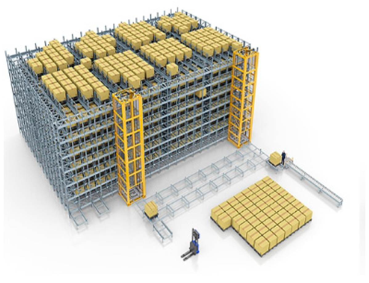
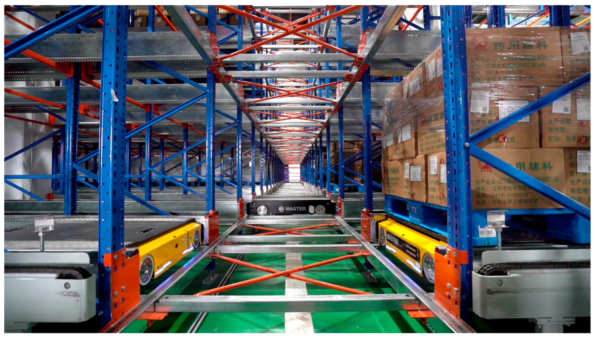
Figure 1 shows a schematic diagram of a four-way shuttle vertical warehouse. The four-way shuttle vertical warehouse is an efficient and flexible automated storage system. Its main hardware components include four-way shuttles, elevators, and racks. The four-way shuttle is the core execution device of the system, responsible for the storage, retrieval, and handling of goods, as shown in Figure 2. Equipped with two pairs of vertical drive wheels, the four-way shuttle can move in four directions. It is also equipped with various sensors (such as lidar, cameras, and ultrasonic sensors) for environmental perception, and can precisely execute handling tasks in combination with the motion control system. 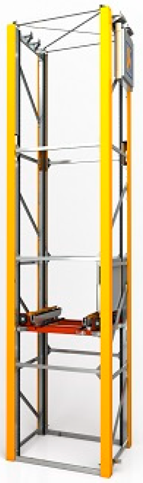As shown in Figure 3, the elevator achieves vertical handling through a cargo platform. The four-way shuttle can enter the cargo platform for handling operations and can also move with the elevator for inter-layer operations. The four-way shuttle rack (as shown in Figure 4) is the main storage device of the system. It adopts a modular design and has high scalability. The rack is composed of columns and beams, and rails are laid between storage locations, forming the driving path for the four-way shuttle to move horizontally.

The software of the four-way shuttle system is mainly the warehouse management system (WMS), which integrates path planning algorithms to solve problems such as multi-vehicle collaboration and task scheduling, ensuring the efficient operation of the warehouse. Compared with the stacker storage system, the four-way shuttle system has a higher storage density and supports the simultaneous operation of multiple four-way shuttles, enabling rapid storage and retrieval, reducing the waiting time for goods, and thus improving the efficiency of inbound and outbound operations. In addition, the four-way shuttle system has good flexibility. It can increase or decrease the number of four-way shuttles according to requirements, adapt to future development, and can flexibly adapt to different warehouse layouts to optimize space utilization. The four-way shuttle system also has real-time monitoring and scheduling capabilities, which can dynamically adjust storage and retrieval strategies, quickly respond to inventory changes and market demands, and improve storage efficiency. The above characteristics make the four-way shuttle system an efficient solution for warehouse expansion and layout changes, meeting the flexibility requirements of modern logistics.

3. System Modeling

Based on the characteristics of the four-way shuttle system, the research in this paper is conducted based on the following assumptions:

• The scene map is represented by a raster graph. Each four-way shuttle in the system has the same model and performance, and the size of one four-way shuttle just occupies one raster.
• Time is represented in a discrete manner. Each four-way shuttle can only move one raster or stay in place within each unit of time. The acceleration of the four-way shuttle is regarded as infinite, and it takes one unit of time to pick and place goods and change directions.
• The four-way shuttle adopts the operation mode of composite tasks. One four-way shuttle can receive multiple composite tasks, but these tasks need to be completed in sequence. Subsequent tasks cannot be executed before all operations of the previous composite task are completed.
• Only the inbound and outbound tasks on a single-layer plane are considered, and the inbound and outbound locations of goods are known. The situation where the target goods in the warehouse need to be relocated during storage and retrieval is not considered.

When the system starts to operate, at t = 0, the WMS evenly distributes all composite tasks to all four-way shuttles at one time. It is assumed that the initial position of all four-way shuttles is at the elevator of the first inbound task. A composite task is composed of one inbound task bound to one outbound task. The four-way shuttle completes the inbound operation, the empty running operation, and the outbound operation in sequence according to the task order. The process of a composite operation is as follows:

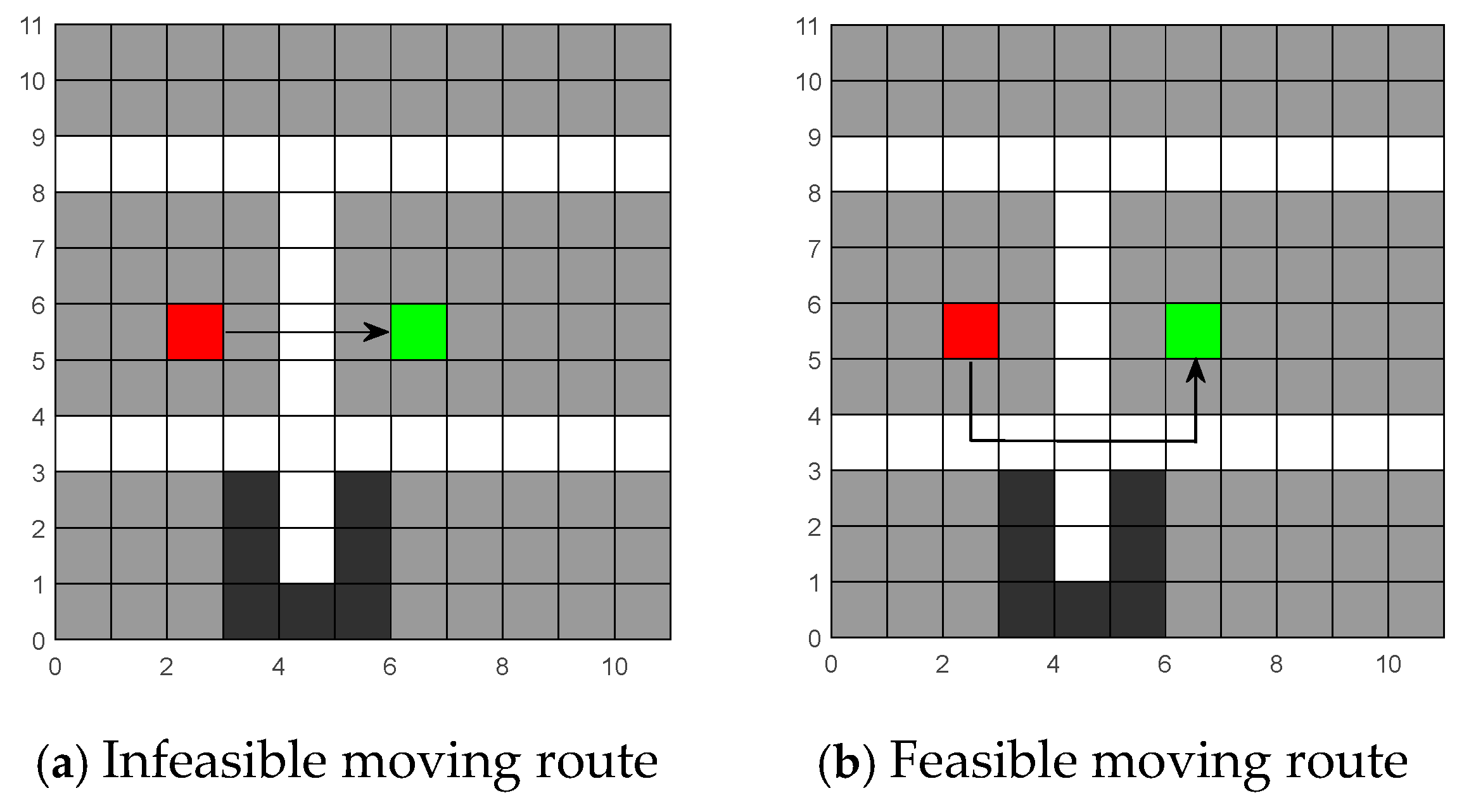
• Inbound operation: The four-way shuttle retrieves the pallet from the elevator docking port. Subsequently, it traverses through the main aisle and sub-aisles, reaching the entrance of the roadway corresponding to the target storage location. After entering the roadway, it arrives at the target storage location and deposits the pallet. If the roadways in columns of this layer are unoccupied and obstacle-free, the four-way shuttle can utilize these roadways as sub-aisles for longitudinal movement.
• Unloaded operation: Upon completion of the inbound operation, the four-way shuttle enters an unloaded state. Based on the location of the goods specified in the outbound task of this composite task, a path from the termination point of the inbound task to the initiation point of the outbound task must be planned. Since the four-way shuttle is not carrying any cargo at this stage, it can pass beneath the storage locations. All roadways can serve as sub-aisles for longitudinal movement.
• Outbound operation: The four-way shuttle picks up the pallet from the outbound storage location and moves to the roadway entrance. Then, it transports the pallet through the main aisle and sub-aisles to the target elevator docking port. Once the unloading process is finished, this composite task concludes. If there are unoccupied and obstacle-free roadways on this layer, the four-way shuttle can employ these roadways as sub-aisles for longitudinal movement.

When, among multiple composite tasks assigned by the warehouse management system (WMS), the elevator for the inbound task of a composite task is in a different position from the elevator for the outbound task of the previous composite task, an empty-running operation is required, and the four-way shuttle is commanded to move to the position of the elevator for the next inbound task.

Now, the representations of the constants, variables, etc. mentioned in the mathematical modeling stage are listed separately here for reference, as shown in

Table 1. Explanation of symbols.

Symbols	The Meaning of the Symbol
a	The operation number executed by the four-way shuttle, where 1 ≤ a ≤ Ni and a ∈ N*
B	The set of obstacle coordinates, generated after initializing the map
C	The cost value for the four-way shuttle to complete all tasks
c	The cost value for the four-way shuttle to execute a certain task
Da	he coordinates of the end point of the a-th operation
Ei	The number of no-load operations to be inserted for the four-way shuttle i
I	The set of numbers of four-way shuttles
$i$	The number of any four-way shuttle, where i ∈ I
$j$	The number of any four-way shuttle, where $j$∈ I and $j$≠ $i$
Li(t)	The location of the four-way shuttle i at time t
Map	The grid map containing information about the number of rows and columns
m	The number of four-way shuttles, where m ∈ N*
Ni	The number of composite tasks assigned to the four-way shuttle i
$P$	The path set of the multi-four-way shuttle system
Pi	The path set of the i-th four-way shuttle, including the coordinate position at each moment
Pi(t)	The position of the four-way shuttle i at time t
Sa	The coordinates of the starting point of the a-th operation
t	Discrete unit time, representing a certain moment
Ti	The task sequence executed by the four-way shuttle i
Wa	The start-end information of the a-th operation of the four-way shuttle
x	Along the row direction of the current layer
y	Along the column direction of the current layer

.

Based on the above assumptions, the path planning problem for multiple four-way shuttles can be described as follows: In the raster map Map, there is a set of obstacle coordinates B, and there are m four-way shuttles, denoted as I = {1, 2, 3, …, m}. The four-way shuttle i needs to execute N_i composite tasks, and E_i empty-running operations need to be inserted between the composite tasks. The task sequence is T_i = {W₁, W₂, W₃, …, W_3Ni+Ei}. The execution of the nth operation W_a by the four-way shuttle i can be expressed as W_a = {S_a, D_a}, where S_a and D_a represent the starting position and the end position of the nth operation respectively. The path of the four-way shuttle i can be expressed as P_i, which records the position of the four-way shuttle i in the map Map at each unit of time. L_i(t) represents the position of the four-way shuttle i at time t, expressed in coordinates (x, y). c(a) represents the cost value of the four-way shuttle executing the task W_a, and C(i) represents the cost value of the four-way shuttle i after executing all tasks, which can be expressed as follows:

$$c\left(a\right)=t_{Da}-t_{Sa}$$

(1)

$$C\left(\mathrm{i}\right)={\sum }_{a=1}^{3N_i+E_i}c\left(a\right)$$

(2)

In the formula, $t_{Sa}$ represents the start time of task a for the four-way shuttle, and $t_{Da}$ represents the end time of task a. For the path planning problem of multiple four-way shuttles, the optimization objective of the mathematical model is to minimize the total task completion time of all four-way shuttles:

$$\min f={\sum }_{i=1}^{m}C\left(i\right)$$

(3)

s.t.

$$L_i\left(t\right)\in Map$$

(4)

$$B\cap P_i\left(t\right)=\varnothing$$

(5)

$$\left|x_i^t-x_i^{t+1}\right|+\left|y_i^t-y_i^{t+1}\right|\le 1$$

(6)

$$P_i\left(t\right)\ne P_j\left(t\right),i\ne j$$

(7)

$$P_i\left(t\right)\ne P_j\left(t+1\right)\wedge P_i\left(t+1\right)\ne P_j\left(t\right),i\ne j$$

(8)

$$\forall i\in \left\{1,2,3,\dots ,m\right\}$$

(9)

$$\forall t\in \left\{0,1,2,3,\dots \right\}$$

(10)

Among the constraint conditions, Equation (4) indicates that the coordinate points of the path of the four-way shuttle must be within the map Map. Equation (5) shows that the path of the four-way shuttle cannot overlap with the obstacle points on the map. Equation (6) represents the movement constraints of the four-way shuttle, which can only move one raster horizontally or vertically per unit of time, or stay in place. Among them, $\left(x_i^t,y_i^{t+1}\right)$ and $\left(x_i^t,y_i^{t+1}\right)$ represent the coordinate positions of the four-way shuttle i at time t and (t + 1). Equations (7) and (8) indicate that the four-way shuttles cannot occupy one raster simultaneously and cannot exchange positions, respectively. Equations (9) and (10) represent the value range of the numbers of the four-way shuttles and the value range of the discrete time series.

By solving the above mathematical model, a conflict-free path set will be obtained, denoted as P:

$$P=\left\{P_1,P_2,P_3,\cdots P_m\right\}$$

(11)

In this paper, a combination of the improved A* algorithm and the CBS algorithm will be adopted to solve this path planning problem. Subsequently, the influence of map state changes on the path will be considered, and a path planning method for dynamic environments will be proposed.

4. Design of the Improved A* Algorithm

4.1. The Basic Principle of the A* Algorithm

The core idea of the A* algorithm is to evaluate the cost of each state or node through a heuristic function and select the search path based on this cost. It starts from the initial node, expands nodes step-by-step, and at each step, selects the node with the minimum cost for expansion until the target node is found.

The A* algorithm uses a cost function to measure the shortest path from the current node to the target node. The goal is to find a shortest path from the starting point to the ending point by minimizing the cost value. The cost function is expressed as follows:

$$f\left(n\right)=g\left(n\right)+h\left(n\right)$$

(12)

where $f\left(n\right)$ is the total estimated cost of the current node. $g\left(n\right)$ is the cost of the path that the current node has already traversed. $h\left(n\right)$ is the heuristic estimated distance from the current node to the target node. Usually, the Euclidean distance, Manhattan distance, etc., are used as the heuristic functions.

$$h\left(n\right)=\sqrt{{\left(x_n-x_g\right)}^2+{\left(y_n-y_g\right)}^2}$$

(13)

$$h\left(n\right)=\left|x_n-x_G\right|+\left|y_n-y_G\right|$$

(14)

In the formulas, $\left(x_n,y_n\right)$ and $\left(x_G,y_G\right)$ represent the coordinates of the current node n and the target node G. Due to the motion characteristics of the four-way shuttle, which moves in four directions on the track and the expansion direction of nodes is also only four without the ability to move diagonally, it is more reasonable to use the Manhattan distance to represent the heuristic function $h\left(n\right)$.

The main process of the A* algorithm is as follows (Algorithm 1):

Algorithm 1: Main process of the A* algorithm

Step 1: Create a map ‘Map’, determine the initial node S and the target node G. Initialize an OPEN List to store the nodes to be evaluated, and put the starting point into the OPEN List. Then, establish a CLOSE List to store the nodes that have been evaluated, so as to avoid repeated evaluation. The CLOSE List is initially empty.

Step 2: Select the node with the minimum cost value $f\left(n\right)$ from the OPEN List and mark this node as the current node. If this node is the target node G, the search is completed and the path is found. Go to Step 5. If it is not the target node, go to Step 3.

Step 3: For each adjacent node of the current node, perform the following steps:

(1) If the adjacent node is in the CLOSE List, skip this node.

(2) If the adjacent node is not in the OPEN List, calculate its $f\left(n\right)$, $g\left(n\right)$, and $h\left(n\right)$ values, and add it to the OPEN List.

(3) If the adjacent node is already in the OPEN List, but the $g\left(n\right)$ value of the current path is smaller, update the cost value of this node and update its parent node.

Step 4: After the current node is processed, move it to the CLOSE List. Return to Step 2.

Step 5: Starting from the target node, trace back the parent node of each node until reaching the starting point to obtain the final shortest path.

4.2. Improvement of the Steering Strategy

The traditional A* algorithm mainly focuses on the total cost of the path while ignoring the smoothness of the path, especially the number of turns in the path, as shown in Figure 5. Two routes pass through the same number of grids from the starting point to the ending point, but the number of turns differs significantly. When considering the cost of the four-way shuttle’s direction change, the more turns there are, the longer the time consumed. To improve this, this study introduces a steering strategy to reduce the number of turns in the path.

In this strategy, a direction-changing penalty is introduced for each expanded node, and the new actual cost function is as follows:

$$g^{\prime }\left(n+1\right)=g\left(n\right)+c+Punish$$

(15)

In the formula, $g\left(n\right)$ is the actual cost of the current node, c is the cost required to move from the current node to the next node, and Punish is the cost of direction change, whose value depends on whether the four-way shuttle changes direction at this node. Here, the judgment of direction change is defined. Let the current node be $\left(x_n,y_n\right)$, its parent node be $\left(x_{n-1},y_{n-1}\right)$, and the expanded child node be $\left(x_{n+1},y_{n+1}\right)$. Then, two vectors and the formula for judging a turn can be obtained, which are expressed as follows:

$$v_1=\left(x_n-x_{n-1},y_n-y_{n-1}\right)$$

(16)

$$v_2=\left(x_{n+1}-x_n,y_{n+1}-y_n\right)$$

(17)

$$v_1·v_2=\left(x_n-x_{n-1}\right)\left(x_{n+1}-x_n\right)+\left(y_n-y_{n-1}\right)\left(y_{n+1}-y_n\right)$$

(18)

If the dot product of the two vectors in Equation (18) is equal to 0, it indicates that the two vectors are perpendicular, meaning that the path has changed direction vertically. In this case, Punish = 1, which means the direction-changing time is one unit of time. The value of Punish is expressed as follows:

$$Punish=\left\{\begin{array}{c}1 { v}_1\cdot v_2=0\\ 0 v_1·v_2\ne 0\end{array}\right.$$

(19)

The value of the heuristic function h(n) affects the final result of the A* algorithm. The improvement of the heuristic function in this paper is as follows:

• When the expanded node and the target node are on the same straight line in the same roadway, there is at least 0 turn, and the value of the heuristic function is as follows:

  $$h^{\prime }\left(n\right)=h\left(n\right)$$

  (20)
• When the expanded node and the target node are on the same straight line in the same roadway, but there are obstacles between the expanded node and the target node, there are at least 3 turns, and the value of the heuristic function is as follows:

  $$h^{\prime }\left(n\right)=h\left(n\right)+3\cdot Punish$$

  (21)
• When the expanded node and the target node are not on the same straight line in the same roadway, there is at least 1 turn, and the value of the heuristic function is as follows:

  $$h^{\prime }\left(n\right)=h\left(n\right)+Punish$$

  (22)

Through these improvements, it is possible to effectively reduce the number of turns in the A* algorithm, thereby optimizing the smoothness of the path and improving the quality of path planning.

4.3. Direction Constraint of Expanded Nodes

Figure 6 is a schematic diagram of the movement route of the four-way shuttle. Since the storage roadways of the four-way shuttle system are longitudinally arranged, the four-way shuttle cannot move left or right within the roadways. Therefore, it cannot directly move to the target point in the way shown in Figure 6a, but can only move in the way shown in Figure 6b. Consequently, it is necessary to introduce the direction constraint of expanded nodes.

Since the four-way shuttle can only select four-direction expanded nodes when moving in the main channel, and can only choose the upward and downward directions in the remaining channels. To determine whether the current node searched by the A* algorithm is located in the main channel, a direction matrix is introduced, and the coordinates of the main channel are identified. The specific representation is as follows:

$$\mathrm{M}=\left[\begin{array}{ccccccc}1& 1& 1& \cdots & 1& 1& 1\\ 1& 1& 1& \cdots & 1& 1& 1\\ 0& 0& 0& \cdots & 0& 0& 0\\ 1& 1& 1& \cdots & 1& 1& 1\\ 1& 1& 1& \cdots & 1& 1& 1\\ 1& 1& 1& \cdots & 1& 1& 1\\ 1& 1& 1& \cdots & 1& 1& 1\\ 0& 0& 0& \cdots & 0& 0& 0\\ 1& 1& 1& \cdots & 1& 1& 1\\ 1& 1& 1& \cdots & 1& 1& 1\\ 1& 1& 1& \cdots & 1& 1& 1\end{array}\right]$$

(23)

In this matrix, the positions occupied by 1 correspond to the coordinates of the rack grids and sub-channels. When the A* algorithm searches for expanded nodes, if the position in the direction matrix corresponding to the coordinates of the current node is 1, only the grids in the upward and downward directions can be selected as expanded nodes. Correspondingly, the positions occupied by 0 in the matrix represent the coordinates of the main channel. If the position in the direction matrix corresponding to the coordinates of the current node is 0, the grids in the upward, downward, left, and right directions can be selected as expanded nodes. The actual cost value corrected by the direction matrix is as follows:

$$g^{″}\left(n+1\right)=g^{\prime }\left(n+1\right)+\left|x_{n+1}-x_n\right|\cdot \left(M\left(x_{n+1},y_{n+1}\right)+M\left(x_n,y_n\right)\right)\cdot R$$

(24)

In the formula, $x_{n+1}$ represents the x-coordinate value of the expanded node, $x_n$ represents the x-coordinate value of the current node, and R is infinity, indicating that the four-way shuttle cannot expand nodes across sub-channels.

5. Optimization of the CBS Algorithm Based on the A* Algorithm

5.1. Basic Principle of the Conflict-Based Search Algorithm

The Conflict-Based Search (CBS) algorithm, as an efficient multi-agent path planning method, aims to find conflict-free paths for multiple agents through two key stages: high-level conflict search and low-level path planning.

In the low-level path planning stage, classic single-agent path planning algorithms such as the A* algorithm are used to plan paths for each agent separately. During this process, the existence of other agents is not considered. Instead, a path from the starting point to the end point is planned based only on the agent’s own starting and target positions.

The high-level conflict search stage focuses on resolving conflicts generated in the low-level path planning. It is achieved by constructing a constraint tree. Initially, each agent obtains a preliminary path through the low-level path planning algorithm. Then, the algorithm comprehensively checks the paths of all agents to identify existing conflicts. These conflicts usually occur when two or more agents are at the same position at the same time or use the same path edge at the same time.

After a conflict is detected, the algorithm decomposes it into specific constraints, mainly including time constraints and space constraints. These constraints are applied to the paths of the conflicting agents respectively. For example, if two agents will meet at the same position at a certain time, a constraint of “not being at this position at this time” will be added to one of the agents.

For agents affected by the constraints, their paths are re-planned in the low-level path planning according to the new constraints. This process still uses the single-agent path planning algorithm, but the newly added constraints are fully considered to avoid previously detected conflicts.

After each application of constraints and re-planning of paths, a new node is generated in the constraint tree. The algorithm continuously checks whether there are still conflicts in the new paths. If there are conflicts, the process of conflict decomposition, constraint application, and path update is repeated until a conflict-free path solution that meets all constraints is found.

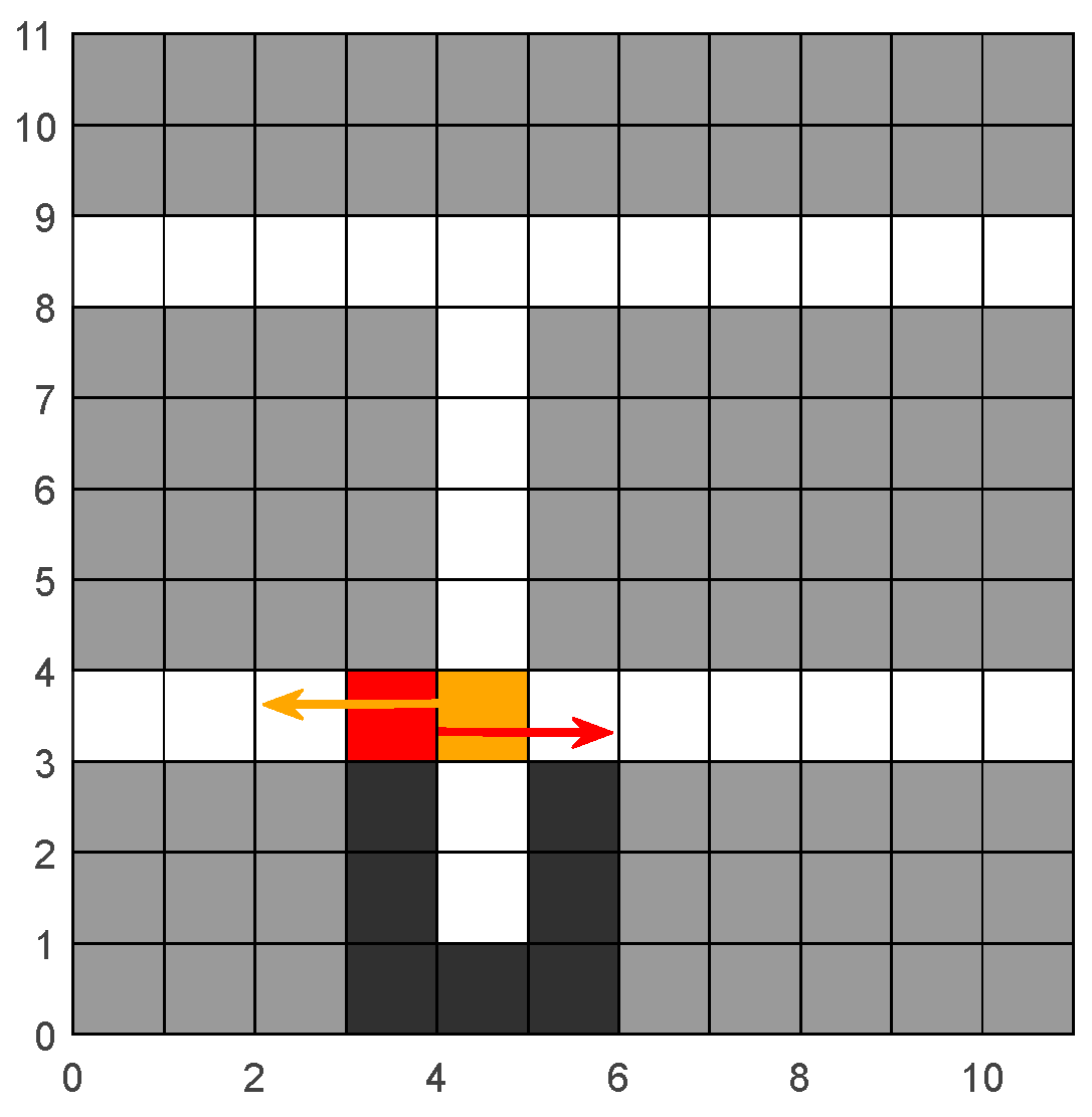
5.2. Conflict Avoidance Strategy

In the problem of path planning for multiple four-way shuttles, the design of conflict avoidance strategies is an important part of ensuring the efficient operation of the system. During the task execution process of four-way shuttles, position conflicts or path conflicts often occur, and at this time, reasonable avoidance strategies must be adopted to solve these problems. This paper proposes two effective conflict avoidance strategies: the priority strategy for inbound and outbound tasks and the priority strategy for nearby tasks. These two strategies can optimize the conflict resolution process in different scenarios and improve the overall efficiency of the system.

5.2.1. The Priority Strategy for Inbound and Outbound Tasks

The core idea of the inbound and outbound task priority strategy is to determine the priority of four-way shuttles based on the types of tasks they are performing, mainly the impact of tasks on the storage location status. Since inbound tasks will occupy storage locations upon completion, they are given priority. For idle-load tasks, as an outbound task will start right after an idle-load task is finished, and the status of the storage location changes at the moment when the four-way shuttle picks up the goods, four-way shuttles performing idle-load tasks also have priority. The main process of the inbound and outbound task priority strategy algorithm is shown in Algorithm 2.

When a conflict occurs between two four-way shuttles, assume that the set of conflicts is “conflicts”, which includes specific conflict instances such as “conflict1” and “conflict2”. Each instance contains the time when the conflict occurs, the location of the conflict, and the numbers of the conflicting four-way shuttles. For each “conflict”, obtain the numbers of the two four-way shuttles involved, denoted as “FS1” and “FS2”. Use the function “DeterminePriority” to determine whether they have priority. This function first checks if they are performing tasks related to changes in the storage location status. If an idle-load task is detected, it further checks the validity of the inbound and outbound tasks before and after this idle-load task (whether the starting point and the ending point are the same) to determine if it is an idle-load task between two compound tasks. If not, it is given priority. After being judged by the function “DeterminePriority”, the priority statuses of FS1 and FS2 are denoted as “priority1” and “priority2” respectively.

Compare the priorities of the two conflicting four-way shuttles. If only one shuttle has priority, the other needs to give way. In the pseudo-code, if “priority1 > priority2”, apply constraints to FS2 using the function “ApplyConstraint(FS2, conflict)” and re-plan the path of FS2 using the A* algorithm. Conversely, if “priority2 > priority1”, apply constraints to FS1 using the function “ApplyConstraint(FS1, conflict)” and re-plan the path of FS1. If neither of the two four-way shuttles is involved in changes to the storage location status, or if both are performing inbound tasks or idle-load tasks, the nearby-task priority strategy is executed.

The advantage of this strategy is that it can flexibly determine the conflict priority according to the nature of tasks. Especially in situations where optimal utilization of storage location resources needs to be ensured, by prioritizing tasks that affect the storage location status, it effectively avoids the waste of storage location resources.

Algorithm 2: Main function of the priority strategy for inbound and outbound tasks

Input: Map, conflict set conflicts = {conflict1, conflict2…}, path set P of four-way shuttle

Output: A set of conflict-free paths P

Initialization: FS1, FS2 1:  for each conflict in conflicts do 2:   FS1 = conflict.shuttle1 3:   FS2 = conflict.shuttle2 4:   priority1 = DeterminePriority(FS1) 5:   priority2 = DeterminePriority(FS2) 6:   if priority1 > priority2 then 7:     ApplyConstraint(FS2, conflict) 8:     shuttle2.path = AStar(FS2, GetConstraints(FS2)) 9:   else if priority2 > priority1 then 10:    ApplyConstraint(FS1, conflict) 11:    shuttle1.path = AStar(FS1, GetConstraints(FS1)) 12:  else 13:    NearbyTaskPriorityStrategy(FS1, FS2, conflict) 14:  end if 15:  end for 16:  return P

5.2.2. The Priority Strategy for Nearby Tasks

The nearby task priority strategy determines the priority in case of conflicts based on the distance between the four-way shuttle and the target location. When a conflict is detected, calculate the Manhattan distances between the two conflicting four-way shuttles and their respective targets. The shuttle with a shorter distance is given a higher priority. Apply constraints to the other four-way shuttle and re-plan its path to make it give way to the shuttle with higher priority. The pseudo-code of the nearby task priority strategy algorithm is shown in Algorithm 3.

First, use the “CalculateDistance” function to calculate the Manhattan distances between FS1, FS2 and their respective targets, and obtain “distance1” and “distance2”. Compare these two distance values. If “distance1” is less than “distance2”, it means FS1 is closer to its target. At this time, give FS1 a higher priority. In the pseudo-code, this is reflected in applying the constraint related to the conflict “conflict” to FS2 using the function “ApplyConstraint(FS2, conflict)”, and then re-planning the path of FS2 using the A* algorithm according to the constraints of FS2. Otherwise, apply the constraint “ApplyConstraint(FS1, conflict)” to FS1 and re-plan the path of FS1.

The underlying assumption of this strategy is that a four-way shuttle closer to its target is usually near the end of its task. If its progress is delayed, it may lead to an overall delay in the task, which in turn affects the system’s efficiency. Therefore, prioritizing the four-way shuttle closer to the target can ensure that the task is completed on time and reduce unnecessary time consumption.

Algorithm 3: Algorithm of the priority strategy for nearby tasks

Input: Map, FS1, FS2, conflict, PFS1, PFS2

Output: A set of conflict-free paths

Initialization: distance1, distance2 1:   distance1 = CalculateDistance(FS1.path, FS1.currentTask.end) 2:   distance2 = CalculateDistance(FS2.path, FS2.currentTask.end) 3:   if distance1 < distance2 then 4:    ApplyConstraint(FS2, conflict) 5:    FS2.path = AStar(FS2, GetConstraints(FS2)) 6:   else 7:    ApplyConstraint(FS1, conflict) 8:    FS1.path = AStar(FS1, GetConstraints(FS1)) 9:   end if 10:  return PFS1, PFS2

In conclusion, the priority strategy for inbound and outbound tasks and the priority strategy for nearby tasks respectively provide different conflict resolution solutions from two perspectives: the impact of tasks on the status of storage locations and the physical distance between tasks and their targets. The former optimizes the use of resources by giving priority to tasks that affect the status of storage locations, while the latter reduces system delays by prioritizing the completion of tasks that are closer to their targets. By flexibly selecting these two strategies in practical applications, the scheduling efficiency and resource utilization rate of the multi-four-way shuttle system can be effectively improved.

5.3. Global Planning of CBS Based on the Dynamic Environment

In this study, the execution of inbound and outbound tasks will lead to changes in the situation of storage locations within the warehouse. There are specifically the following two situations:

• After the inbound task is completed, the roadway that was originally unoccupied by goods is occupied. A four-way shuttle carrying goods can no longer use this roadway as a sub-channel for movement.
• After the outbound task starts, the roadway that was originally occupied by only one storage location is released from occupation. There are no goods in this roadway, and a four-way shuttle carrying goods can use this roadway as a sub-channel for movement.

These two situations will cause the originally planned path to no longer be the optimal path. To solve this problem, this paper proposes a global planning of CBS based on the dynamic environment, and the basic principles are as follows:

Step 1: Combine the known task set into composite tasks in the form of inbound tasks, empty-running tasks, and outbound tasks, and evenly distribute them to all four-way shuttles. If the end position of the previous composite task of a four-way shuttle is different from the start position of the next composite task, add an empty-running task to move to the start position of the next composite task.

Step 2: Initialize the map and plan the path, and import two rasterized maps:

• Import the information of the positions where goods are already stored in the warehouse and the obstacles into the rasterized map. When inbound and outbound tasks occur, the A* algorithm calls this map to plan the path for the four-way shuttle.
• Only import the information of the obstacles in the warehouse into the rasterized map. When an empty-running task occurs, the A* algorithm calls this map to plan the path for the four-way shuttle.

Step 3: Establish a ChangeList. This list records, in ascending order of time points, the types of inbound and outbound tasks completed by all four-way shuttles, the time points when the map changes occur, the corresponding coordinates, and the numbers of the four-way shuttles.

Step 4: Conflict detection. Conduct conflict detection according to the path of each obtained four-way shuttle. Check whether there are situations of position exchange (Figure 7) or simultaneous occupation of one raster (Figure 8) on the path. Record the obtained first conflict position, time point, and the number of the four-way shuttle, and proceed to Step 5. If no conflict is detected, proceed to Step 8.

Step 5: Compare the conflict time with the time recorded in the first set of data in the ChangeList. If the conflict time is less than the time in the list, it indicates that the conflict occurred before the map state changed. At this time, check whether the number of the four-way shuttle recorded in the first set of the list is the same as that of the four-way shuttle involved in the conflict. If it is, proceed to Step 6; if not, proceed to Step 7. If the conflict time is greater than the time in the list, proceed to Step 9.

Step 6: Adopt the priority strategy for inbound and outbound tasks. Add constraints to the non-priority four-way shuttle for avoidance and use the A* algorithm to replan the path to resolve the conflict. Return to Step 4.

Step 7: Adopt the priority strategy for nearby tasks. Assign priority to the four-way shuttle closer to the destination. Add constraints to the other four-way shuttle for avoidance and use the A* algorithm to replan the path. Then, return to Step 4.

Step 8: Check if the ChangeList is empty. If it is empty, it means that the map state has been fully changed and there are no conflicts in the paths of the four-way shuttles. The algorithm ends, and a conflict-free path solution set is obtained. If it is not empty, proceed to Step 9.

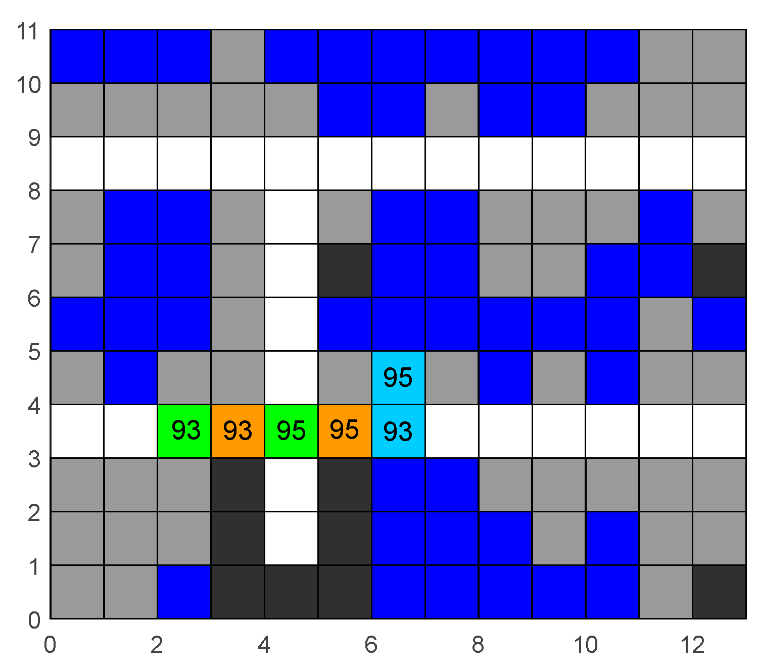
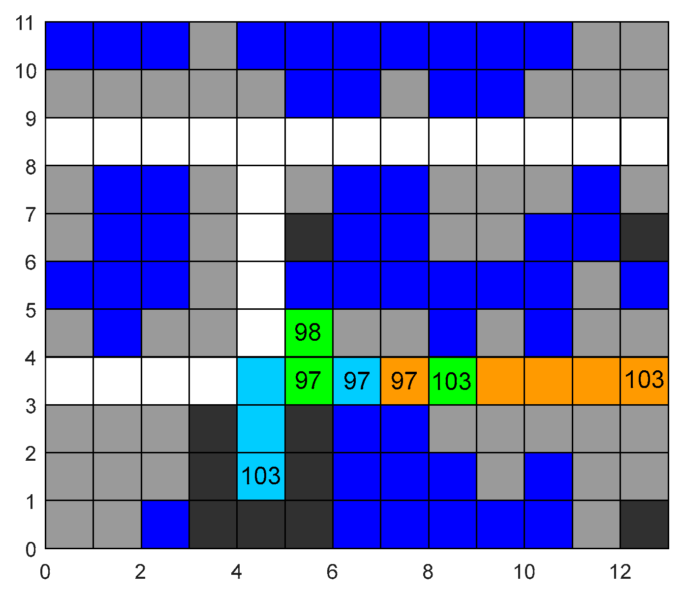
Step 9: Update the map and replan the paths. According to the task type and coordinates in the first set of data in the ChangeList, modify the distribution state of obstacles on the map. Due to the change in the occupancy of storage locations in the warehouse, replan the path for each four-way shuttle. Specifically, the four-way shuttle that causes the map change by completing a task replans the path for subsequent tasks using the new map, while the path before this task remains unchanged. For other four-way shuttles, take the position at the time point when the map changes as the starting point, and replan the path to complete the current task and subsequent tasks. Update the completion time points of subsequent tasks in the ChangeList and then delete the first set of data in the ChangeList and return to Step 4.

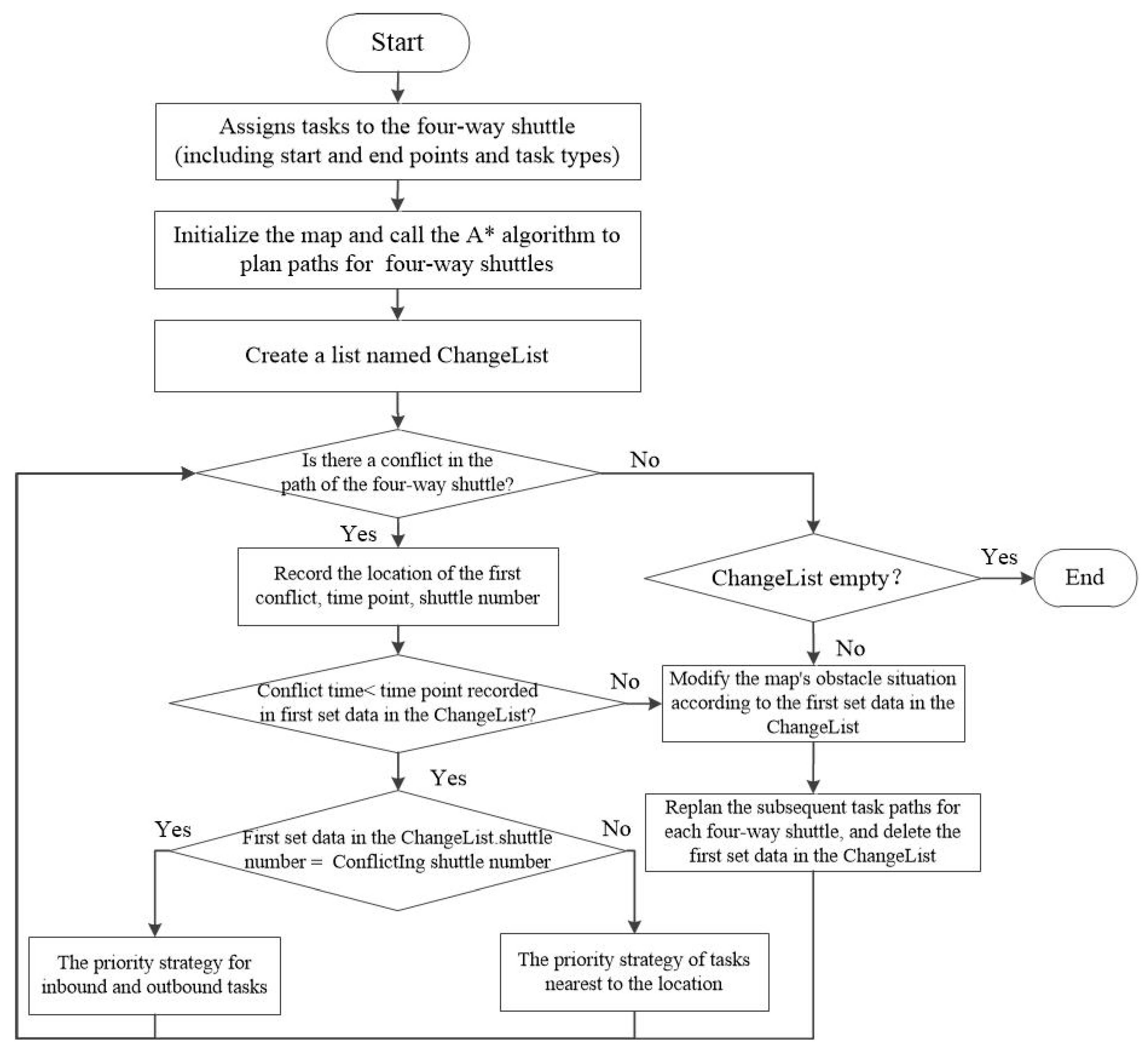
Figure 9 shows the flowchart of the global planning algorithm of CBS based on the dynamic environment.

6. Simulation Experiment

6.1. Parameter Settings for the Simulation Experiment

To deeply explore the effectiveness of this algorithm in path searching, this study conducts experimental analysis based on the layout of the four-way shuttle vertical warehouse of an enterprise. Matlab 2016b software is selected as the main simulation and data analysis platform. With its powerful matrix operation capabilities, rich function libraries, and convenient visualization tools, Matlab software provides efficient support for the simulation of complex algorithms and data processing.

In terms of hardware tools, a high-performance computer device is relied on to run Matlab software. This computer is equipped with an Intel Xeon E5 processor, has 32 GB of running memory and a 512 GB solid-state drive, ensuring the efficient and stable operation of large-scale data operations and complex model construction during the simulation experiment.

In this experiment, using the image processing and matrix operation functions of Matlab, an 11-row × 25-column environmental model of the four-way garage is constructed through the grid method. In the constructed environmental model, it includes three elevators and three four-way shuttles. The initial storage situation in the warehouse is shown in Figure 10. In the figure, the blue grids represent occupied storage locations, the gray grids represent idle storage lanes, the black grids represent fixed obstacles, and the white grids represent the main passageways for the four-way shuttles. At the same time, to simulate the actual operation scenario, two composite tasks are generated, and the task allocation of the four-way shuttles is shown in

Table 2. Basic experimental settings.

Number	Four-Way Shuttle-1	Four-Way Shuttle-2	Four-Way Shuttle-3	Task Type
1	(5,2)→(10,6)	(15,11)→(6,10)	(24,2)→(18,1)	Inbound
2	(10,6)→(4,7)	(6,10)→(10,2)	(18,1)→(12,1)	Empty
3	(4,7)→(5,2)	(10,2)→(15,11)	(12,1)→(24,2)	Outbound
4	(5,2)→(5,2)	(15,11)→(8,11)	(24,2)→(11,11)	Inbound
5	(5,2)→(15,11)	(8,11)→(2,1)	(11,11)→(12,6)	Empty
6	(15,11)→(15,11)	(2,1)→(15,11)	(12,6)→(5,2)	Outbound
7	(15,11)→(3,1)			Inbound
8	(3,1)→(13,6)			Empty
9	(13,6)→(24,2)			Outbound

.

Initially, each of the three four-way shuttles was assigned six tasks, including two inbound tasks, two empty-running tasks, and two outbound tasks. Since the end position of the first composite task of the No. 1 four-way shuttle was different from the starting position of the second composite task, an empty-running task was added to move the No. 1 four-way shuttle. Specifically, an empty-running composite task was inserted, as shown by task numbers 4–6 of the No. 1 four-way shuttle in Table 2.

6.2. Verification of the Improved A* Algorithm

In reference [20], the Manhattan distance of A was weighted in the form of a weighting coefficient to increase the influence of the abscissa for turning. This algorithm is denoted as IA*-1. To verify the effectiveness of the improvement of the cost function in the improved A* algorithm proposed in this paper (hereinafter referred to as IA*), five sets of tasks with initial positions and end positions were randomly generated based on the initial storage location state in Figure 10. The computational effects of the traditional A* algorithm, IA*, and IA*-1 were compared through experiments. The three algorithms were run respectively to solve the generated task data. The experimental results are shown in

Table 3. Comparison table of the improved A* algorithm.

Number	Task Points	A*		IA*		IA*-1
		Cost	Nodes	Cost	Nodes	Cost	Nodes
1	(22,1)→(5,11)	31	98	29	89	29	104
2	(2,1)→(15,11)	27	91	25	84	25	97
3	(5,2)→(18,8)	25	88	23	75	23	91
4	(9,10)→(20,5)	21	85	19	66	19	88
5	(21,6)→(3,10)	30	93	30	87	30	98

and Figure 11.

In Figure 11, the starting and ending points of the four-way shuttle are (22,1) and (5,11) respectively. When using the A* algorithm to solve for the path, the four-way shuttle makes 4 turns, the path length is 27, and when the turning cost is 1, the total cost value of the path is 31, with the number of expanded nodes being 98. When using the IA* algorithm for solving, the number of turns is 2, the total cost value of the path is 29, and the number of expanded nodes is 89. Compared with the traditional A* algorithm, the computational efficiency and path optimization results of IA* are significantly improved.

Table 3 shows the optimization results of different algorithms. From the perspective of considering the cost value of turns, the path optimization results obtained by the IA* algorithm and IA*-1 are consistent, and both are superior to the traditional A* algorithm. However, in terms of the number of nodes, IA* has the least number of expanded nodes, followed by the traditional A* algorithm and the IA*-1 algorithm. This indicates that after the improvement of the heuristic function in IA*, more heuristic information is provided, which helps to accelerate the search efficiency. After the heuristic function of the IA*-1 algorithm is weighted, the heuristic information is reduced, and more nodes need to be expanded to meet the path search requirements. In summary, IA* has better search efficiency and path search ability, and is suitable as a basic algorithm for the path planning research of multiple four-way shuttles.

6.3. Analysis of the Simulation Results

Input the tasks in Section 6.1 into the algorithm model. The paths and task durations for each four-way shuttle to complete the tasks are shown in

Table 4. Experimental results of four-way shuttle (No. 1).

Number	Path of Four-Way Shuttle	Path Length	Stop Times	Task Duration	Time Node
1	(5,2)→(5,4)→(10,4)→(10,6)	9	4	13	13
2	(10,6)→(10,8)→(4,8)→(4,7)	11	2	13	26
3	(4,7)→(4,4)→(5,4)→(5,2)	6	4	10	36
4	(5,2)	0	0	0	36
5	(5,2)→(5,4)→(15,4)→(15,8)→(15,11)	20	4	24	60
6	(15,11)	0	0	0	60
7	(15,11)→(15,9)→(4,9)→(4,4)→(3,4)→(3,1)	22	6	28	88
8	(3,1)→(3,4)→(13,6)	15	2	17	105
9	(13,6)→(13,4)→(24,4)→(24,2)	15	4	19	124

,

Table 5. Experimental results of four-way shuttle (No. 2).

Number	Path of Four-Way Shuttle	Path Length	Stop Times	Task Duration	Time Node
1	(15,11)→(15,9)→(6,9)→(6,10)	12	4	16	16
2	(6,10)→(6,8)→(6,9)→(10,9)→(10,2)	14	5	19	35
3	(10,2)→(10,4)→(15,4)→(15,11)	14	4	18	53
4	(15,11)→(15,9)→(8,9)→(8,11)	11	4	15	68
5	(8,11)→(8,4)→(2,4)→(2,1)	16	2	18	86
6	(2,1)→(2,4)→(6,4)→(6,5)→(6,4)→(15,4)→(15,11)	25	7	32	118

and

Table 6. Experimental results of Four-way shuttle (No. 3).

Number	Path of Four-Way Shuttle	Path Length	Stop Times	Task Duration	Time Node
1	(24,2)→(24,4)→(18,4)→(18,1)	11	4	15	15
2	(18,1)→(18,4)→(12,4)→(12,1)	12	2	14	29
3	(12,1)→(12,4)→(24,4)→(24,2)	17	4	21	50
4	(24,2)→(24,9)→(11,9)→(11,11)	22	4	26	76
5	(11,11)→(11,9)→(12,9)→(12,6)	6	2	8	84
6	(12,6)→(7,4)→(7,5)→(7,4)→(5,4)→(5,2)	13	6	19	103

. Here, the path length refers to the number of grids passed from the starting point to the ending point. The number of stops includes the times when the four-way shuttle lifts and lowers the goods, stays in place to avoid obstacles, and changes directions, with each stop consuming 1 unit of time. The task duration is the unit time consumed to complete a task, and the time node is the cumulative global time after completing a certain task. At the end of the experiment, the final time t = 124, and the final storage location state is shown in Figure 12.

6.4. Analysis of the Algorithm’s Effectiveness

This section will analyze the influence of the CBS global planning in the dynamic environment on the path selection of each four-way shuttle during a specific period in the experimental process of the parameters in Section 6.1. The main scenarios include the impact of the changes in the roadway status caused by inbound and outbound operations on the path, the priority strategy for inbound and outbound operations, and the influence of the priority strategy of tasks in the vicinity on the paths of the four-way shuttles.

6.4.1. Influence of Roadway State Changes on Path Planning

According to Task 1 of the No. 1 four-way shuttle in Table 4, the inbound operation is completed at t = 13, and the storage location at coordinates (10,6) is occupied. Referring to the initial state of the warehouse in Figure 10, after this time point, the roadway with x = 10 and y = 5–8 will no longer be an empty roadway. Subsequently, the loaded four-way shuttles will not choose this roadway as a sub-channel for longitudinal movement.

The specific manifestations can be referred to in Figure 13 and Figure 14. In this figure and the figures in the subsequent text, the orange grids represent the path of the No. 1 four-way shuttle, the green grids represent the path of the No. 2 four-way shuttle, and the light blue grids represent the path of the No. 3 four-way shuttle. According to the path of Task 3 of the four-way shuttle in Table 5, from t = 36 to 53, the No. 2 four-way shuttle executes the outbound Task No. 3, and the path is (10,2)→(10,4)→(15,4)→(15,11). The CBS global planning algorithm based on the dynamic environment updates the obstacle map after the inbound and outbound operations are completed, so that the coordinate (10,6) is occupied, and the subsequent path is re-planned. The original path of the No. 2 four-way shuttle from (10,2) to (10,9) (Figure 13) becomes unavailable, realizing the path update.

Similarly, if an empty roadway is created after the completion of an outbound task, the loaded four-way shuttle can use it as a sub-channel for movement. As shown in Tasks No. 2 and 3 in Table 4, after the no-load task ends at t = 26, the outbound task starts at t = 27. The four-way shuttle carries the outbound pallet. After t = 27, the storage location (4, 7) is released. Referring to the initial state of the warehouse in Figure 10, the roadway with x = 4 and y = 5–8 will become an empty roadway. The results of the specific path updates due to the map changes are shown in Figure 14 and Figure 15. From t = 69 to 86, the No. 1 four-way shuttle is executing the inbound Task No. 7, and the No. 2 four-way shuttle is executing the no-load Task No. 5.

The path without considering the dynamic environment is shown in Figure 15. The No. 1 four-way shuttle selects the sub-channel for longitudinal movement, and the path is (10,9)→(5,9)→(5,4)→(3,4)→(3,2). The CBS global planning based on the dynamic environment removes the goods at (4,7), making the roadway with x = 4 and y = 5–8 passable, as shown in Figure 16. Since the turning cost is added to the A* algorithm, when expanding nodes, the feasible nodes that do not require turning will be preferentially selected. Therefore, when the No. 1 four-way shuttle is at the position (5,9), both the paths in Figure 15 and Figure 16 are passable and have the same cost. The A* algorithm will preferentially select the path shown in Figure 16, which does not require turning at this node.

6.4.2. The Influence of the Priority Strategy on Path Planning

To intuitively demonstrate the effects of the inbound-outbound priority strategy and the nearby-task priority strategy on the path planning of four-way shuttles, take the map states during the time periods of t = 89–92, t = 93–95, and t = 96–103 as examples.

When t = 89–92, as shown in Figure 17, the No. 1 four-way shuttle is performing the no-load Task No. 8, and the No. 2 four-way shuttle is performing the outbound Task No. 6. At t = 92, the No. 1 four-way shuttle changes direction and needs to stay at (3,4) for one unit of time. At this time, if there is no interference, the position of the No. 2 four-way shuttle should also be (3,4), resulting in a conflict where the positions of the No. 1 and No. 2 four-way shuttles overlap. According to the inbound-outbound priority strategy, the No. 1 four-way shuttle is performing a no-load task. After the no-load task is completed, the outbound task will start, which will cause a change in the storage location state. So, it is the four-way shuttle about to cause a storage location change, and it is given the path priority. Constraints are imposed on the underlying A* algorithm of the No. 2 four-way shuttle, so that the No. 2 four-way shuttle cannot choose (3,4) as an extended path at t = 92. The No. 2 four-way shuttle stays in place for one unit of time.

Similarly, as shown in Figure 18, from t = 93–95, the No. 3 four-way shuttle is performing the outbound Task No. 6. Without interference, its position should be (6,4) at t = 94. When t = 95, it will exchange positions with the No. 1 four-way shuttle, resulting in a conflict. Since the No. 1 four-way shuttle has priority, the No. 3 four-way shuttle performs avoidance.

When t = 96, the positions of each four-way shuttle are shown in Figure 19. At the next moment, the No. 1 four-way shuttle will move to (8,4). Without interference, both the No. 2 and No. 3 four-way shuttles will move to (7,4), and at this time, their positions will overlap, and a conflict will occur. Since both the No. 2 and No. 3 four-way shuttles are performing outbound tasks at this moment, they do not meet the conditions for the priority four-way shuttle in the inbound-outbound priority strategy. Therefore, the nearby-task priority strategy is invoked here. The target position of the No. 2 four-way shuttle is (15,11), and the target position of the No. 3 four-way shuttle is (5,2). The No. 3 four-way shuttle is closer to its target, so it has priority.

The paths after resolving the conflict based on priority are shown in Figure 20. When t = 97, the No. 2 four-way shuttle changes direction, the No. 3 four-way shuttle moves to (7,4), and the No. 1 four-way shuttle moves in the direction of (13,4). When t = 98, the No. 2 four-way shuttle moves to (6,5) to perform avoidance, and the No. 3 four-way shuttle moves to (6,4). During the time period from t = 98 to 103, no conflict occurs. The path of the No. 2 four-way shuttle is (6,5)→(6,4)→(9,4). The path of the No. 3 four-way shuttle is (6,4)→(5,4)→(5,2).

6.4.3. Analysis of the Algorithm’s Scalability

In order to comprehensively evaluate the scalability and practical application potential of the algorithm proposed in this paper in complex dynamic environments, this paper systematically increases the number of four-way shuttles and the scale of tasks. The proposed algorithm is then subjected to a multi-dimensional comparative analysis with the classic path planning algorithms, namely the D* Lite algorithm and the RRT algorithm, to deeply explore the performance change trends of different algorithms under different scales.

In reference [21], the time dimension and turning cost were introduced into the nodes of the D* Lite algorithm, and the improved algorithm was integrated into the CBS to propose the DCBS algorithm. Furthermore, by adding the real-time repulsive force of adjacent agents, the DCBS-PFM algorithm was proposed to achieve conflict avoidance in dynamic environments. Reference [22] proposed a hybrid method that combines the Artificial Potential Field (APF) method and the RRT path planning algorithm (hereinafter referred to as RRT-A). The weight factor of this hybrid method is determined according to the layout of the current obstacles.

To analyze the performance of the algorithms, an experiment was conducted using the initial map in Figure 10. For each four-way shuttle, three composite tasks were randomly generated and executed. By changing the number of four-way shuttles in the system, the performance of the dynamic environment path planning algorithm based on A* and CBS proposed in this paper (hereinafter referred to as IA*-CBS) was compared with that of DCBS-PFM and RRT-A. During the experiment, it was assumed that the initial position of the four-way shuttles was at the elevator. When the number of four-way shuttles was greater than three, in order to simulate the scenario of multi-batch task issuance in actual warehouses and avoid instantaneous traffic congestion caused by the concentrated start of vehicles, three four-way shuttles were first allowed to start working, and five unit times later, the remaining four-way shuttles were allowed to start working. The results of the algorithm performance indicators for different numbers of four-way shuttles are shown in

Table 7. The algorithm performance under different numbers of four-way shuttles.

Number of Four-Way Shuttles	Algorithm	Average Calculation Time	Average Task Completion Time	Average Number of Conflicts	Average Number of Direction Changes
3	IA*-CBS	45.6 s	172.4 s	14.5	69.4
	DCBS-PFM	34.1 s	177.3 s	15.2	72.1
	RRT-A	43.7 s	182.6 s	14.7	76.2
4	IA*-CBS	62.8 s	185.8 s	19.3	96.4
	DCBS-PFM	46.3 s	190.4 s	26.1	97.3
	RRT-A	65.2 s	197.2 s	24.5	100.2
5	IA*-CBS	97.4 s	190.6 s	29.7	142.6
	DCBS-PFM	63.6 s	194.9 s	34.2	146.5
	RRT-A	96.2 s	199.3 s	31.6	149.1

. For the experimental results under each number of four-way shuttles, the average value was taken after 10 experiments. In the table, the average task completion time refers to the average value of the end times when the system completed all tasks in each experiment, which reflects the length of the planned path. The average number of conflicts is the average value of the number of times the algorithm resolves conflicts in each experiment, which reflects the ability and efficiency of the algorithm in handling conflicts during multi-agent path planning. The lower this value is, the more effectively the algorithm can coordinate the driving paths of multiple four-way shuttles during path planning, reducing the collisions or intersection conflicts between vehicles. The average number of direction changes is the average value of the total number of direction changes of all four-way shuttles in each experiment, which reflects the smoothness of the path.

The experimental results indicate that the IA*-CBS algorithm demonstrates certain advantages in multi-dimensional performance. In terms of the average task completion time, as the number of four-way shuttles increases from 3 to 5, the task completion time of the IA*-CBS algorithm remains at a relatively low level. For instance, when the number of four-way shuttles is 5, the average task completion time of the IA*-CBS algorithm is 190.6 s, which is more efficient compared to 194.9 s of the DCBS-PFM algorithm and 199.3 s of the RRT-A algorithm. This suggests that the IA*-CBS algorithm can plan paths with better lengths and effectively improve the operation efficiency of multiple vehicles.

Regarding the average number of conflicts, the IA*-CBS algorithm also shows certain competitiveness. When the number of four-way shuttles is 3, the average number of conflicts of the IA*-CBS algorithm is 14.5 times, lower than 15.2 times of the DCBS-PFM algorithm and 14.7 times of the RRT-A algorithm. When the number of vehicles increases to 5, the number of conflicts of the IA*-CBS algorithm is 29.7 times, slightly lower than those of the other two algorithms. This indicates that the IA*-CBS algorithm has a certain effect in coordinating the driving paths of four-way shuttles and reducing vehicle conflicts.

Moreover, the paths planned by the IA*-CBS algorithm exhibit good smoothness. Under different numbers of four-way shuttles, its average number of direction changes is lower than those of the DCBS-PFM and RRT-A algorithms, which helps to reduce the energy consumption and mechanical wear of four-way shuttles during operation.

However, there is room for improvement in the computational efficiency of the IA*-CBS algorithm. Since it needs to continuously conduct conflict searches and path re-planning, as the number of four-way shuttles gradually increases, its computational time also increases significantly. Further optimization of the algorithm’s efficiency is required to enhance its practicality.

6.4.4. Summary of Algorithm Analysis

Based on the above experimental results, the IA* algorithm with the steering strategy and node expansion direction constraints has stronger path planning capabilities and higher computational efficiency compared to the traditional A* algorithm and the IA*-1 algorithm.

Using IA* as the underlying algorithm, the CBS algorithm is improved. By analyzing the paths of the four-way shuttles during the time periods of t = 36–53 and t = 69–86 in the simulation results and comparing them with the paths planned without using the map update strategy, the effectiveness of the map update method in the CBS global planning algorithm based on the dynamic environment is verified. By analyzing the paths of each four-way shuttle during the time period of t = 89–103, the implementation effects of the inbound-outbound priority strategy and the nearby-task priority strategy are demonstrated, and the effectiveness of the obstacle-avoidance function for multiple four-way shuttles in the CBS global planning algorithm based on the dynamic environment is verified.

In the comparative experiments with the DCBS-PFM and RRT-A algorithms, the IA*-CBS algorithm demonstrated excellent performance. It features a relatively short average task completion time, enabling efficient path planning; a lower average number of conflicts, indicating good vehicle coordination ability; and a low average number of direction changes, suggesting good path smoothness. Although there is still room for optimization in terms of computational efficiency, overall, it shows reliable performance in multiple dimensions and has strong application potential.

7. Conclusions

To address the multi-vehicle path planning problem in a four-way shuttle storage system within a dynamic environment, considering the map state changes caused by the inbound and outbound operations of four-way shuttles, a CBS global planning algorithm based on the dynamic environment is proposed. This algorithm improves the CBS obstacle-avoidance algorithm based on the A* algorithm. By adding direction constraints for expanding nodes and turning costs, the path search ability and computational efficiency of the A* algorithm are enhanced. A ChangeList is introduced to record the task type, time point, coordinates, and the number of the four-way shuttle for each task when the map state changes. By updating the ChangeList, the paths of other four-way shuttles after the map state change are re-planned, enabling the paths of four-way shuttles to be updated according to environmental changes.

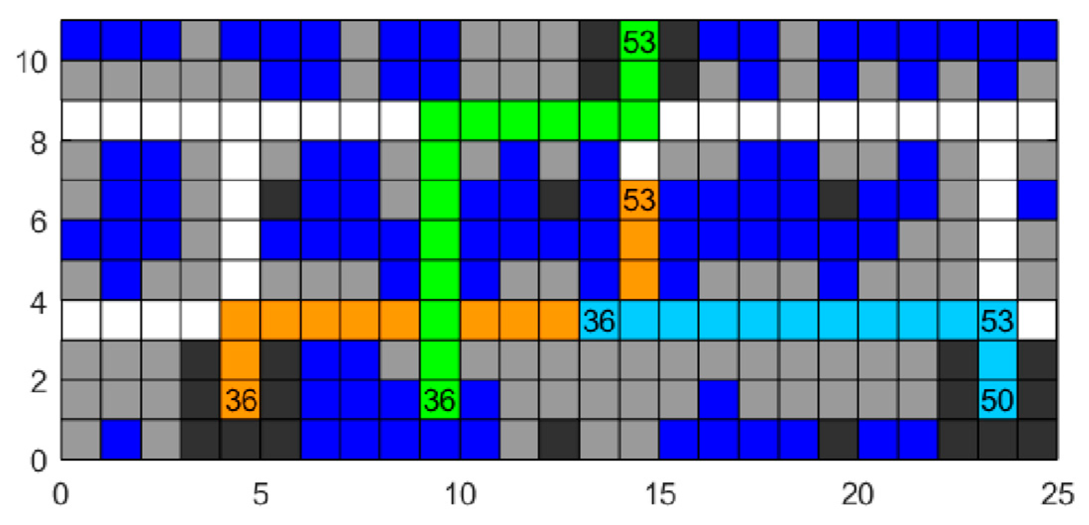
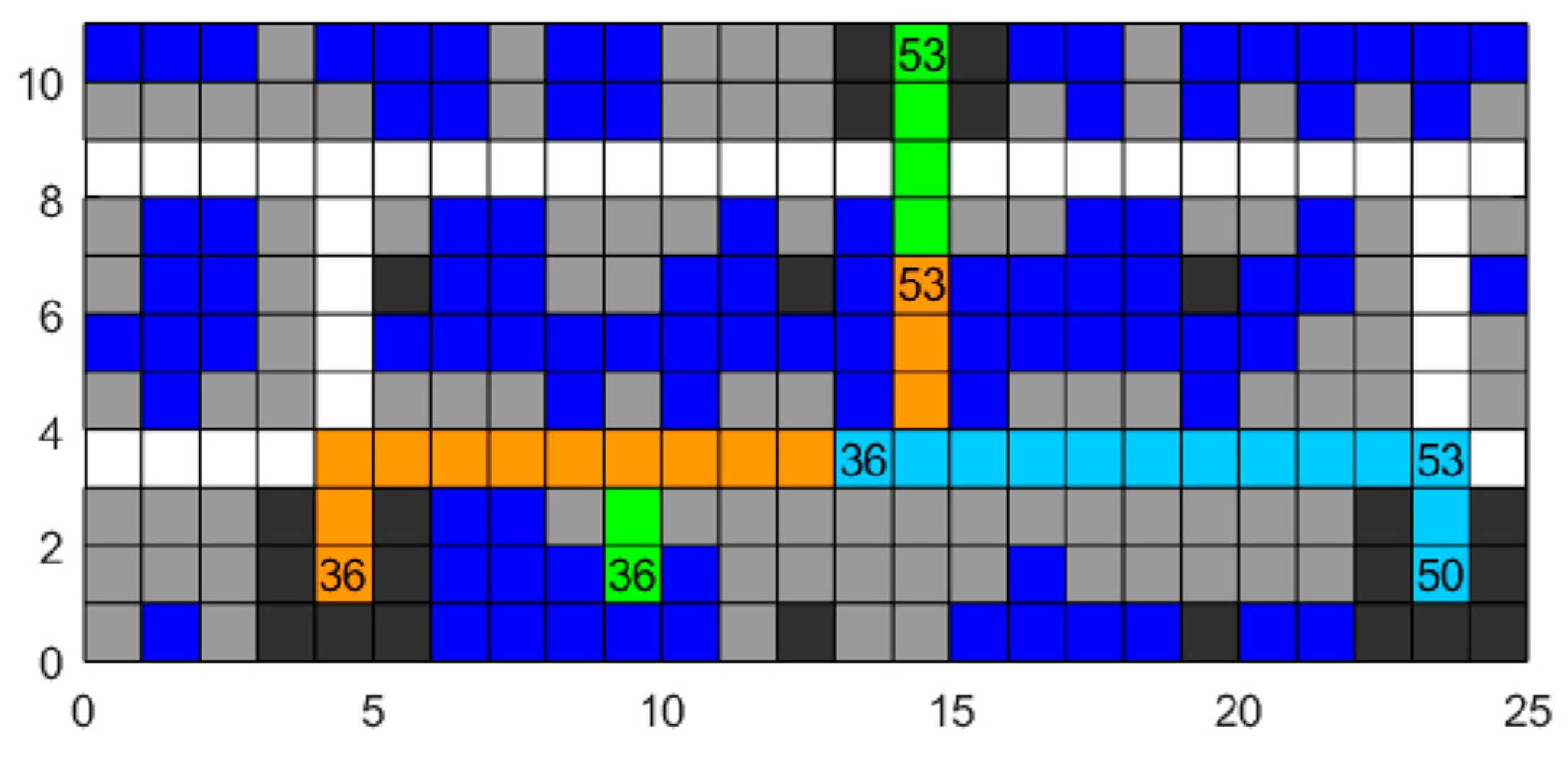
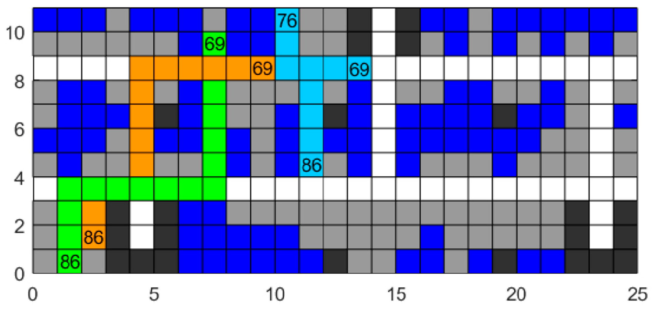
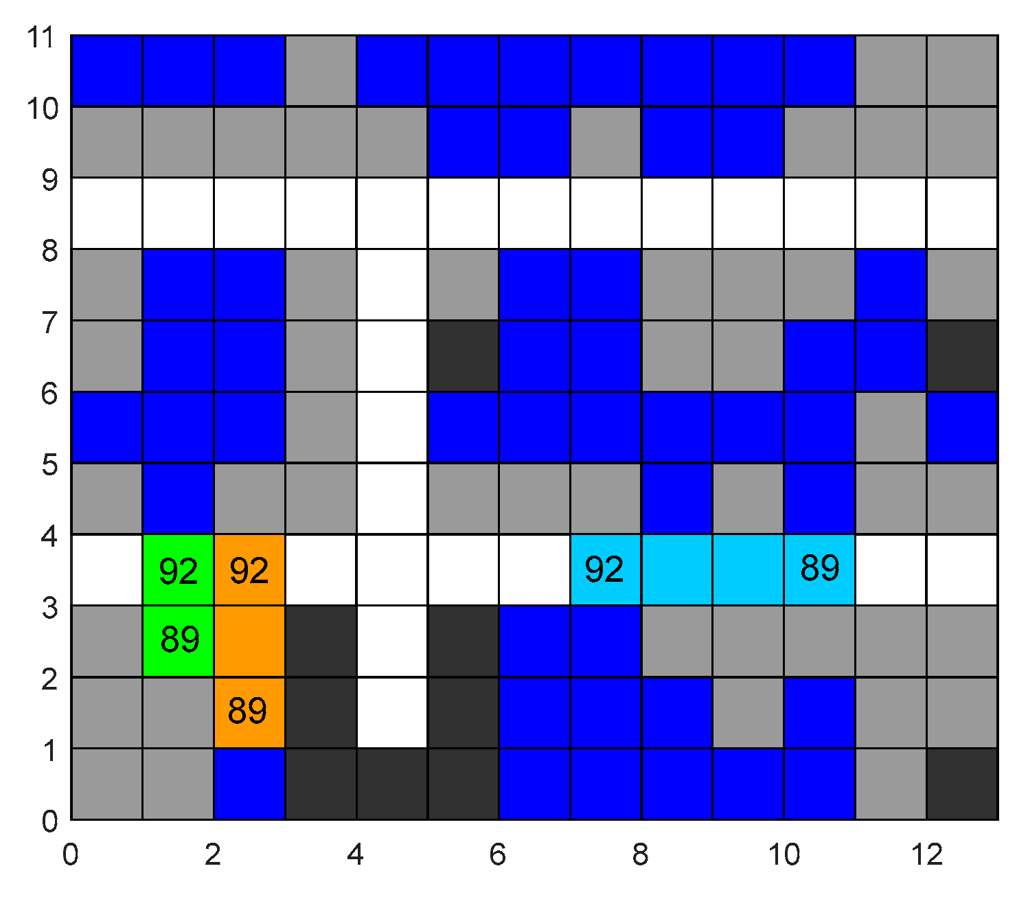
In terms of conflict resolution, the inbound-outbound task priority strategy and the nearby-task priority strategy are incorporated into the CBS algorithm, resulting in a set of conflict-free paths that take into account both dynamic map changes and obstacle avoidance for multiple four-way shuttles. By referencing the layout of a four-way shuttle warehouse of a certain company and conducting simulation analysis, a conflict-free path set is obtained when three four-way shuttles operate simultaneously, each with two sets of composite tasks. The effectiveness of the algorithm is verified by analyzing the path status of four-way shuttles during specific time periods.

In the comparative experiments with algorithms such as DCBS-PFM and RRT-A, the IA*-CBS algorithm proposed in this paper demonstrated excellent performance. It performed outstandingly in key indicators such as the average task completion time, the average number of conflicts, and the average number of direction changes. It is capable of efficiently planning paths, effectively reducing vehicle conflicts, and decreasing vehicle energy consumption, which reflects its strong competitiveness and practical application potential.

This study did not consider the acceleration and deceleration issues of four-way shuttles, as well as the collaborative scheduling problems with elevators. To conform to the actual operation situation of the system, further research can incorporate more rigorous equipment parameters into the calculation of equipment path costs, such as acceleration and deceleration rates, direction change time, pallet lifting time, etc., and conduct scheduling research on the entire four-way shuttle system in combination with the connection between the elevators and the four-way shuttles. At the same time, considering that there is still room for optimization in the computational efficiency of the current algorithm, it is necessary to further explore optimization strategies to improve the algorithm’s operation efficiency, so as to better meet the practical needs of the actual warehouse system.

References

1. Borovinsek, M.; Ekren, B.Y.; Burinskiene, A.; Lerher, T. Multi-objective Optimisation Model of Shuttle-based Storage and Retrieval System. Transport 2017, 32, 120–137. [Google Scholar] [CrossRef]
2. Koenig, S.; Likhachev, M.; Furcy, D. Lifelong planning A∗. Artif. Intell. 2004, 155, 93–146. [Google Scholar] [CrossRef]
3. Shankar, M.; Sushnigdha, G. A Hybrid Path planning approach combining Artificial Potential Field and Particle Swarm Optimization for Mobile Robot. IFAC-PapersOnLine 2022, 55, 242–247. [Google Scholar] [CrossRef]
4. Dewang, H.S.; Mohanty, P.K.; Kundu, S. A Robust Path Planning for Mobile Robot Using Smart Particle Swarm Optimization. Procedia Comput. Sci. 2018, 133, 290–297. [Google Scholar] [CrossRef]
5. Lamini, C.; Benhlima, S.; Elbekri, A. Genetic Algorithm Based Approach for Autonomous Mobile Robot Path Planning. Procedia Comput. Sci. 2018, 127, 180–189. [Google Scholar] [CrossRef]
6. Lin, S.; Liu, A.; Wang, J.; Kong, X. An intelligence-based hybrid PSO-SA for mobile robot path planning in warehouse. J. Comput. Sci. 2023, 67, 101938. [Google Scholar] [CrossRef]
7. Zhang, J.; Zhang, F.; Liu, Z.; Li, Y. Efficient Path Planning Method of USV for Intelligent Target Search. J. Geovisualization Spat. Analysis 2019, 3, 13. [Google Scholar] [CrossRef]
8. Guo, C.; Li, D.M.; Zhang, G.L.; Zhai, M.L. Real-Time Path Planning in Urban Area via VANET-Assisted Traffic Information Sharing. IEEE Trans. Veh. Technol. 2018, 67, 5635–5649. [Google Scholar] [CrossRef]
9. Aine, S.; Sujit, P.B. Integrating planning and control for efficient Path planning in the presence of environmental disturbances. In Proceedings of the 26th International Conference on Automated Planning and Scheduling, ICAPS 2016, London, UK, 12–17 June 2016. [Google Scholar] [CrossRef]
10. Eran, C.; Keskin, M.O.; Cantürk, F.; Aydogan, R. A Decentralized Token-Based Negotiation Approach for Multi-Agent Path Finding. In Proceedings of the 18th European Conference on Multi-Agent Systems (EUMAS), Virtual Event, 28–29 June 2021. [Google Scholar] [CrossRef]
11. Wei, C.Y.; Hindriks, K.V.; Jonker, C.M. Altruistic coordination for multi-robot cooperative pathfinding. Appl. Intell. 2016, 44, 269–281. [Google Scholar] [CrossRef]
12. Pianpak, P.; Son, T.C. DMAPF: A Decentralized and Distributed Solver for Multi-Agent Path Finding Problem with Obstacles. In Proceedings of the 37th International Conference on Logic Programming (ICLP), Porto, Portugal, 20–27 September 2021. [Google Scholar] [CrossRef]
13. Fransen, K.J.C.; van Eekelen, J.A.W.M.; Pogromsky, A.; Boon, M.A.A.; Adan, I.J.B.F. A dynamic path planning approach for dense, large, grid-based automated guided vehicle systems. Comput. Oper. Res. 2020, 123, 105046. [Google Scholar] [CrossRef]
14. Lee, C.K.M.; Lin, B.B.; Ng, K.K.H.; Lv, Y.Q.; Tai, W.C. Smart robotic mobile fulfillment system with dynamic conflict-free strategies considering cyber-physical integration. Adv. Eng. Inform. 2019, 42, 100998. [Google Scholar] [CrossRef]
15. Lopez, F.G.; Abbenseth, J.; Henkel, C.; Dorr, S. A predictive online path planning and optimization approach for cooperative mobile service robot navigation in industrial applications. In Proceedings of the 2017 European Conference on Mobile Robots (ECMR), Paris, France, 6–8 September 2017. [Google Scholar] [CrossRef]
16. Cao, J. Researches on Robot Path Planning Method Based on Deep Reinforcement Learning in Dynamic Environment. Master’s Thesis, Zhejiang University, Hangzhou, China, 2024. [Google Scholar] [CrossRef]
17. Deng, F.; Guan, H.; Tan, C.; Fu, L.; Wang, H.; Lin, T.; Zhang, J. Multi-robot reinforcement learning path planning method based on request-response communication mechanism and local attention mechanism. J. Comput. Appl. 2024, 44, 432–438. [Google Scholar]
18. Yu, L.; Wang, Y.; Sheng, Z.; Xu, P.; He, Z.; Du, H. Path Planning for Multi-AGV Systems Based on Globally Guided Reinforcement Learning Approach. In Proceedings of the 2024 IEEE International Conference on Unmanned Systems (ICUS), Nanjing, China, 18–20 October 2024. [Google Scholar] [CrossRef]
19. Li, J.Y.; Rum, W.; Koenig, S. EECBS: A Bounded-Suboptimal Search for Multi-Agent Path Finding. In Proceedings of the 35th AAAI Conference on Artificial Intelligence/33rd Conference on Innovative Applications of Artificial Intelligence/11th Symposium on Educational Advances in Artificial Intelligence, ELECTR NETWORK, Virtual, 2–9 February 2021. [Google Scholar]
20. Wu, T. Four-way Shuttle System Configuration and Route Optimization. Master’s Thesis, Jilin University, Changchun, China, 2021. [Google Scholar] [CrossRef]
21. Wang, X. Real-Time Multi-Agent Path Planning in Dynamic Environments with Conflict-Based Search. Master’s Thesis, Qingdao University of Science and Technology, Qingdao, China, 2024. [Google Scholar] [CrossRef]
22. Lee, C.-C.; Song, K.-T. Path Re-Planning Design of a Cobot in a Dynamic Environment Based on Current Obstacle Configuration. IEEE Robot. Autom. Lett. 2023, 8, 1183–1190. [Google Scholar] [CrossRef]
Figure 1. Image of four-way shuttle storage system.
Mathematics 13 01588 g001
Figure 2. Image of four-way shuttle.
Mathematics 13 01588 g002
Figure 3. Image of elevator.
Mathematics 13 01588 g003
Figure 4. Image of four-way shuttle racks.
Mathematics 13 01588 g004
Figure 5. Paths with different turning times.
Mathematics 13 01588 g005
Figure 6. Four-way shuttle moving route.
Mathematics 13 01588 g006
Figure 7. Conflict of position exchange.
Mathematics 13 01588 g007
Figure 8. Conflict of occupying consent grid.
Mathematics 13 01588 g008
Figure 9. Flowchart of CBS global planning algorithm based on dynamic environment.
Mathematics 13 01588 g009
Figure 10. Initial location status of Four-way shuttle system.
Mathematics 13 01588 g010
Figure 11. Comparison diagram of the A* algorithm and the IA* algorithm.
Mathematics 13 01588 g011
Figure 12. The status of the storage location at the end of the experiment.
Mathematics 13 01588 g012
Figure 13. Four-way shuttle trajectory without updated: t = 36–53.
Mathematics 13 01588 g013
Figure 14. Four-way shuttle trajectory after updating: t = 36–53.
Mathematics 13 01588 g014
Figure 15. Four-way shuttle trajectory without updated: t = 69–86.
Mathematics 13 01588 g015
Figure 16. Four-way shuttle trajectory after updating: t = 69–86.
Mathematics 13 01588 g016
Figure 17. Four-way shuttle trajectory: t = 89–92.
Mathematics 13 01588 g017
Figure 18. Four-way shuttle trajectory: t = 93–95.
Mathematics 13 01588 g018
Figure 19. Four-way shuttle trajectory: t = 96.
Mathematics 13 01588 g019
Figure 20. Four-way shuttle trajectory: t = 97–103.
Mathematics 13 01588 g020