Sliding Mode Control Method Based on a Fuzzy Logic System for ROVs with Predefined-Time Convergence and Stability

Abstract

This paper presents a predefined-time control approach to address slow convergence and instability in the orbit control of remotely operated vehicles (ROVs). The proposed method introduces tunable predefined-time stability (PTS), allowing precise adjustment of the system’s stability time through configurable parameters, thereby enhancing controller adaptability. A control input system ensures PTS is developed, while a fuzzy logic system (FLS) is employed to estimate unstructured uncertainties and disturbances. This integration improves robustness, reduces chattering, and eliminates singularities, making the approach well suited for systems with incomplete or unknown model data. Comprehensive simulations validate the effectiveness of the proposed method, demonstrating superior performance compared to existing control strategies and highlighting its potential for advanced ROV applications.

1. Introduction

The ocean, especially its deep-sea regions, holds an abundance of biological and mineral resources. Sustainable exploration, development, and utilization of these resources are vital for advancing societal progress and ensuring long-term environmental sustainability. ROVs, which are unmanned underwater systems, operate through cables connecting them to a surface control station. These cables facilitate real-time transmission of control commands and data collection. Due to their capability for live data feedback and seamless switching between automated and manual control modes, ROVs are often preferred over autonomous underwater vehicles (AUVs) for certain underwater tasks [1].

Developing a robust controller for ROVs is a complex task due to the presence of model uncertainties and unpredictable external forces. The dynamics of an ROV are characterized by strong nonlinearity and coupling, with hydrodynamic parameters typically derived from simulations or experimental tests, which often fail to capture real-world conditions accurately [2]. Moreover, ROVs operating in ocean environments must contend with external influences such as waves and currents, adding further unpredictability to their behavior. These challenges limit the capabilities of conventional linear control techniques, making them inadequate for delivering the precise motion control required for stable and responsive ROV operations [3].

In recent years, a variety of control strategies have been implemented to enhance the performance of ROVs, including PID control [4], a hierarchical control scheme [5], sliding mode control (SMC) [6], and adaptive control [7]. While these methods have been effective to some extent, they commonly rely on asymptotic Lyapunov stability analysis to address the trajectory tracking problem, implying that the tracking error only approaches zero as time approaches infinity. However, in practical applications, achieving a rapid and stable response is crucial for effective ROV trajectory tracking. This underscores the importance of developing control systems capable of ensuring finite-time convergence for ROVs, enabling faster and more reliable operation.

With the growing advancements in finite-time control theory [8,9], numerous finite-time controllers have been developed and implemented for nonlinear systems such as nonlinear multiagent systems [10], nonstrict-feedback nonlinear systems [11], and the control of underwater robots. For instance, a study on a finite-time tracking control method for AUVs without velocity state measurements was presented in [12]. In [13], an adaptive sliding mode strategy was employed for the guidance and control of an underwater hexapod robot. Similarly, Ref. [14] addressed a formation control problem for a swarm of AUVs with nonlinear dynamic uncertainties and environmental disturbances. Based on the leaderless consensus framework, a distributed finite-time event-triggered formation control method was proposed for AUVs, considering collision avoidance. Although these finite-time control methods effectively reduce system errors to zero within a finite time, their performance is significantly influenced by the system’s initial state. When the initial state deviates substantially from the equilibrium point, the convergence time increases markedly. To address this limitation, fixed-time control strategies were introduced for nonlinear systems [15,16,17] including AUVs [18,19], which ensure that convergence time is independent of the system’s initial state. However, these methods come with their own challenges. Specifically, estimating the convergence time requires complex calculations involving multiple control parameters that cannot be directly adjusted by the designer. Any modifications to these parameters may significantly alter the controller’s convergence performance, complicating the rational allocation of convergence time.

To overcome these challenges, a more advanced concept, known as the predefined-time control strategy, has been developed [20,21,22]. This innovative approach enables designers to specify the convergence time as a preset parameter, ensuring that the system achieves convergence within a predefined duration. Moreover, it provides the flexibility to fine-tune the convergence time, offering enhanced control performance and practicality in various applications.

Recent studies have explored predefined-time methods for controlling nonlinear systems, such as underwater robots [23,24] and rigid spacecraft [25], highlighting their ability to adjust convergence time through tunable time parameters. However, these methods face challenges, including complex designs and overly conservative convergence time estimates, often leading to suboptimal performance. For instance, Ref. [23] proposed a predefined-time nonsingular fast terminal sliding mode control for ROV trajectory tracking, focusing solely on the reaching phase while neglecting predefined-time convergence of the sliding motion phase and failing to address chattering. Similarly, Ref. [24] introduced a predefined-time stability control using a conventional sliding mode surface, which does not guarantee predefined-time stability.

One of the primary challenges affecting the operational performance of ROVs is the presence of unknown components, which is further complicated by external factors such as waves and currents that influence their dynamics. To address system uncertainties and ensure convergence in dynamic environments, researchers have developed nonlinear observers and advanced localization techniques. For example, Ref. [26] proposes an innovative observer-based localization scheme that leverages parallel robot kinematics, making it particularly suitable for systems operating in GPS-denied environments. Similarly, Ref. [27] presents a finite-time sliding mode control framework specifically designed for underwater vehicles in 3D space, effectively addressing both robustness and convergence speed. In addition, advanced learning techniques, including fuzzy logic systems (FLSs) [28,29,30,31] and neural networks [9,16,32], have been proposed to further enhance adaptability and estimation capabilities. Iterative learning methods have proven effective in nonlinear systems, enhancing adaptability and overall performance. For instance, Ref. [33] developed an adaptive fuzzy-based finite-time control strategy for chaotic systems, specifically designed to handle full-state constraints and unmodeled dynamics. Adaptive neural networks have been specifically designed for ROV applications, allowing them to learn from their environment and improve responses over time [34]. Additionally, adaptive fuzzy logic systems (AFLSs) integrate human insights into ROV dynamics, enhancing the accuracy of FLS and enabling real-time adaptation to changing conditions [1,19]. The emergence of adaptive fixed-time fuzzy logic controllers combines the benefits of fixed-time convergence with the flexibility and robustness of FLS, leading to improved control strategies for managing the complexities of ROV operations in unpredictable marine environments.

Building on this analysis, this paper proposes a predefined-time control strategy aimed at enhancing trajectory tracking for ROVs, with the following key contributions:

• A novel approach is introduced in predefined-time control design, making it more practical and efficient. This method ensures precise tunability of the system states’ convergence time, effectively addressing the challenges associated with fixed-time designs.
• The proposed predefined-time control method is based on an advanced terminal sliding mode control (TSMC) framework, ensuring nonsingular and fast convergence. The controller dynamically adjusts the dominant convergence term based on configurable parameters. Consequently, the actual convergence time closely aligns with the predefined target, significantly improving the accuracy and reliability of convergence time adjustments.
• This study also introduces an AFLS that enhances system performance by improving robustness, reducing chattering, and eliminating singularities. The AFLS effectively estimates unstructured model uncertainties and compounded disturbances, seamlessly integrating these factors into the control framework.
• A rigorous stability analysis of the proposed strategy is conducted, demonstrating its tunability in achieving predefined convergence times. Extensive comparative simulation experiments validate the effectiveness and superiority of the proposed control scheme, showcasing its ability to provide fast, stable, and precise trajectory tracking for ROVs.

The remainder of this paper is organized as follows: Section 2 introduces the foundational theories of predefined-time convergence and presents the proposed lemma along with its proof. Section 3 outlines the ROV dynamic model. Section 4 details the design process of the proposed method, providing rigorous evidence of its tunable convergence time and stability. Section 5 evaluates the proposed controller through two simulation examples. Finally, Section 6 concludes the paper.

2. Preliminaries and Problem Formulation

For $i=1,2,\dots ,n$ and vectors $\mathbf{x}={[x_1,\dots ,x_n]}^T\in {\mathbb{R}}^n$ and $\mathbf{a}={[a_1,\dots ,a_n]}^T\in {\mathbb{R}}^n$ with $a_i>0$, we define ${\left[\mathbf{x}\right]}^{\mathbf{a}}=[|x_1{|}^{a_1}\mathrm{sign}\left(x_1\right),\dots ,|x_n{{|}^{a_n}\mathrm{sign}\left(x_n\right)]}^T$, $|{x_i}^{a_i}|=|x_i{|}^{a_i}\mathrm{sign}\left(x_i\right)$, ${\left[\mathbf{x}\right]}^{{\alpha }_1}=[|x_1{|}^{{\alpha }_1}\mathrm{sign}\left(x_1\right),\dots ,|x_n{{|}^{{\alpha }_1}\mathrm{sign}\left(x_n\right)]}^T$, and $\mathit{\varphi }=\mathrm{diag}({\varphi }_1,\dots ,{\varphi }_n)$ denotes the diagonal matrix, while $\parallel ·\parallel$ represents the Euclidean norm. Additionally, ${\parallel ·\parallel }_F$ represents the Frobenius norm.

Definitions and Lemmas

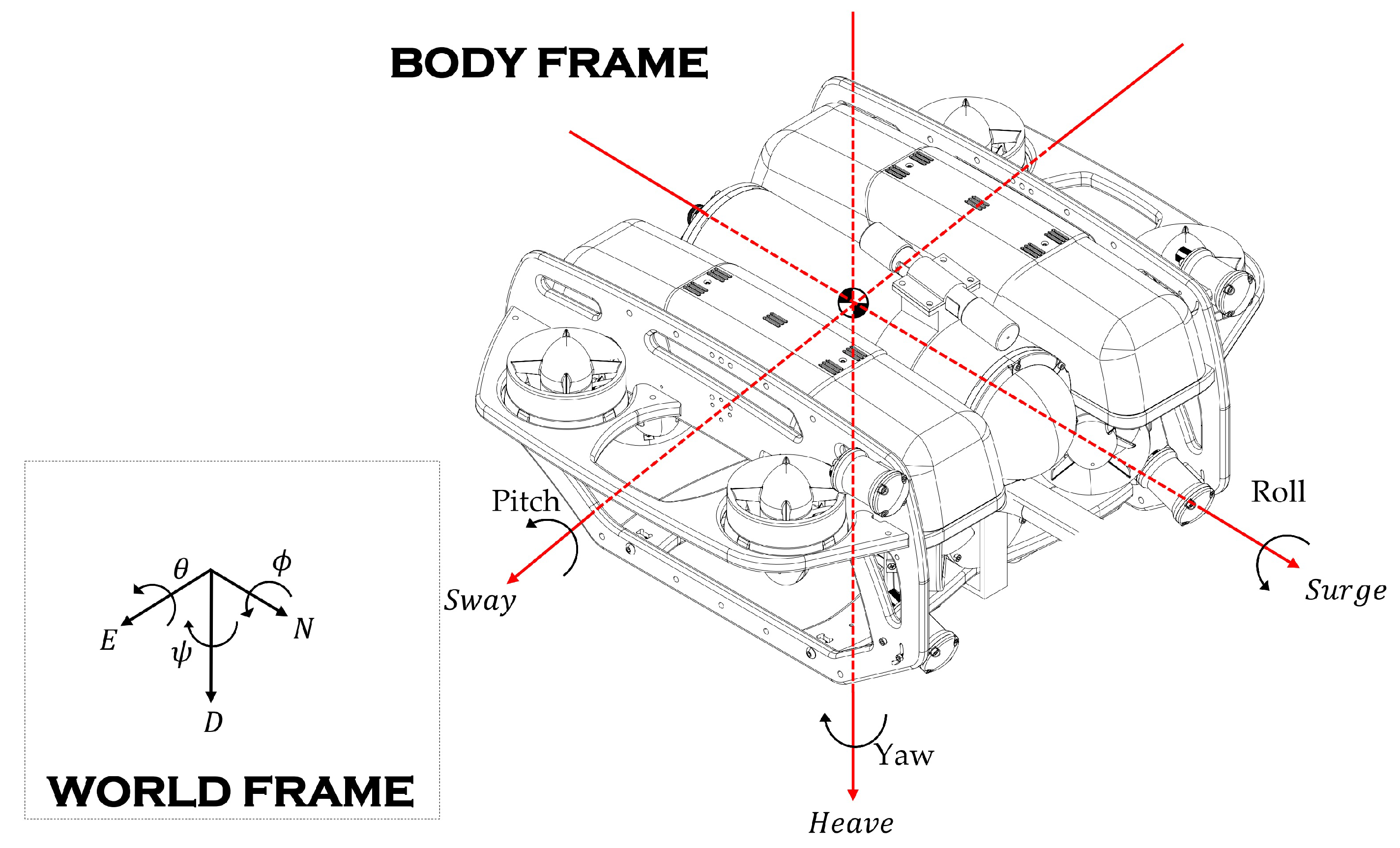
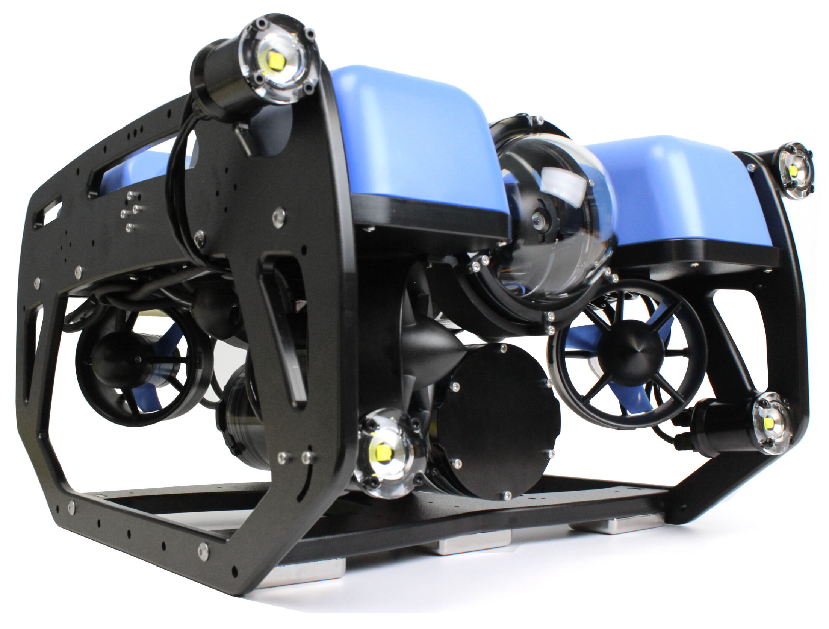
Let us examine the following system:

$$\dot{x}=f\left(x\right),x\left(0\right)=x_0,$$

(1)

where $f:{\mathbb{R}}^n\to {\mathbb{R}}^n$ is a nonlinear function that is continuous, with the condition $f\left(0\right)=0$. The variable $x\in \mathbb{R}$ indicates the system’s states.

Definition 1

([35]). Consider the equilibrium point of the system defined in Equation (1). If this equilibrium point can be stabilized in a finite amount of time and there exists a continuous-time function $T(x_0,\mu ):{\mathbb{R}}^n\to \mathbb{R}$ such that $T(x_0,\mu )\le T_c$ for every $x_0\in {\mathbb{R}}^n$, then the point is referred to as tunably predefined-time stable for the system in (1). Here, $T_c$ denotes a specified time, and μ is a parameter that can be adjusted.

Lemma 1.

Consider a positive definite function $V\left(x\right)$ associated with the system described by Equation (1), defined over a set U where $U_0\subseteq U$ and $x\in U_0\setminus \left\{0\right\}$. Assume that $V\left(x\right)$ fulfills the following condition:

$$\dot{V}\le -{\displaystyle \frac{2\pi \Im }{T_c}}\left({\sigma }_{1}V+{\sigma }_2{V}^{{\displaystyle \frac{3-\alpha }{2}}}+{\sigma }_3{V}^{{\displaystyle \frac{1+\alpha }{2}}}\right),$$

(2)

where $0<\alpha <1$, $T_c>0$ is a specified time, ${\sigma }_1,{\sigma }_2,{\sigma }_3>0$ are constants that satisfy ${\sigma }_1^2\le 4{\sigma }_2{\sigma }_3$, and $\Im ={\displaystyle \frac{1}{(1-\alpha )\sqrt{4{\sigma }_2{\sigma }_3-{\sigma }_1^2}}}$. Under these conditions, the system in Equation (1) is considered tunably predefined-time stable, with $T_c$ serving as the predefined time.

Proof. 

Equation (2) can be express as follows:

$$dV\le -{\displaystyle \frac{2\pi \Im }{T_c}}{V}^{{\displaystyle \frac{\alpha +1}{2}}}\left({\sigma }_1{V}^{{\displaystyle \frac{1-\alpha }{2}}}+{\sigma }_2{V}^{1-\alpha }+{\sigma }_3\right)dt.$$

(3)

Rewrite Equation (3) as follows:

$$\begin{array}{cc}\hfill -{\displaystyle \frac{\pi \Im }{T_c}}dt& \ge {\displaystyle \frac{dV}{2V^{\frac{\alpha +1}{2}}\left({\sigma }_1{V}^{\frac{1-\alpha }{2}}+{\sigma }_2{V}^{1-\alpha }+{\sigma }_3\right)}}\hfill \\ \hfill & \ge {\displaystyle \frac{1}{1-\alpha }}{\displaystyle \frac{d{V}^{\frac{1-\alpha }{2}}}{\left({\sigma }_1{V}^{\frac{1-\alpha }{2}}+{\sigma }_2{V}^{1-\alpha }+{\sigma }_3\right)}}\hfill \end{array}.$$

(4)

Let $T^{*}$ denote the time at which the system stabilizes, such that $V\left(T^{*}\right)=0$ and $V\left(0\right)=V_0>0$.

By integrating from 0 to $T^{*}$, the following expression can be derived:

$$-{\displaystyle \frac{\pi \Im }{T_c}}{\displaystyle \underset{0}{\overset{T^{*}}{\int }}}dt\ge {\displaystyle \frac{1}{1-\alpha }}{\displaystyle \underset{V\left(0\right)}{\overset{V\left(T^{*}\right)}{\int }}}{\displaystyle \frac{d{V}^{\frac{1-\alpha }{2}}}{\left({\sigma }_1{V}^{\frac{1-\alpha }{2}}+{\sigma }_2{V}^{1-\alpha }+{\sigma }_3\right)}},$$

(5)

then

$${\displaystyle \frac{\pi \Im }{T_c}}{\displaystyle \underset{0}{\overset{T^{*}}{\int }}}dt\le {\displaystyle \frac{1}{1-\alpha }}{\displaystyle \underset{0}{\overset{V_0}{\int }}}{\displaystyle \frac{d{V}^{\frac{1-\alpha }{2}}}{\left({\sigma }_1{V}^{\frac{1-\alpha }{2}}+{\sigma }_2{V}^{1-\alpha }+{\sigma }_3\right)}}.$$

(6)

The solution of Equation (6) leads to the following inequality:

$$\begin{array}{cc}\hfill {\displaystyle \frac{\pi \Im }{T_c}}{T}^{*}& \le {\displaystyle \frac{2}{(1-\alpha )\sqrt{4{\sigma }_2{\sigma }_3-{\sigma }_1^2}}}\left(\mathrm{atan}\left({\displaystyle \frac{2{\sigma }_2{V}_0+{\sigma }_1}{\sqrt{4{\sigma }_2{\sigma }_3-{\sigma }_1^2}}}\right)-\mathrm{atan}\left({\displaystyle \frac{{\sigma }_1}{\sqrt{4{\sigma }_2{\sigma }_3-{\sigma }_1^2}}}\right)\right)\hfill \\ \hfill & \le 2\Im \mathrm{atan}\left({\displaystyle \frac{2{\sigma }_2{V}_0\sqrt{4{\sigma }_2{\sigma }_3-{\sigma }_1^2}}{(4{\sigma }_2{\sigma }_3+2{\sigma }_2{V}_0{\sigma }_1)}}\right).\hfill \end{array}$$

(7)

Since $\mathrm{atan}\left({\displaystyle \frac{2{\sigma }_2{V}_0\sqrt{4{\sigma }_2{\sigma }_3-{\sigma }_1^2}}{(4{\sigma }_2{\sigma }_3+2{\sigma }_2{V}_0{\sigma }_1)}}\right)\in (0,{\displaystyle \frac{\pi }{2}})$, and it is monotonically increasing, its maximum possible value is ${\displaystyle \frac{\pi }{2}}$. Thus, we obtain the final bound:

$$\begin{array}{cc}\hfill T^{*}& \le T_c.\hfill \end{array}$$

(8)

Thus, according to Definition 1 and Equation (8), Equation (1) is considered tunably predefined-time stable, where $T_c$ represents the predefined time.    □

3. Modeling of ROV

ROV Dynamic Model

The ROV operates with six degrees of freedom underwater, comprising three axes of translational movement and three axes of rotational motion. Figure 1 illustrates the reference and world frames, showing all degrees of freedom associated with the ROV. For the simplification of calculations, the motion parameters of the ROV are summarized in

Table 1. Motion and force parameters of the underwater vehicle.

Motion Parameters				Force Parameters
Motion	Parameter	Velocity	Parameter	Force Type	Parameter
Surge	x	Surge Velocity	u	Surge Force	X
Sway	y	Sway Velocity	v	Sway Force	Y
Heave	z	Heave Velocity	w	Heave Force	Z
Roll	$\varphi$	Roll Velocity	p	Roll Moment	K
Pitch	$\theta$	Pitch Velocity	q	Pitch Moment	M
Yaw	$\psi$	Yaw Velocity	r	Yaw Moment	N

. The kinematic equation governing its motion is expressed as follows:

$$\dot{\mathit{\eta }}=\mathit{J}\left(\mathit{\eta }\right)\mathit{v}.$$

(9)

The pose of the ROV is represented by $\mathit{\eta }={\left[\begin{array}{cccccc}x& y& z& \varphi & \theta & \psi \end{array}\right]}^T\in {\mathbb{R}}^{6\times 1}$, where ${\mathit{\eta }}_1={\left[\begin{array}{ccc}x& y& z\end{array}\right]}^T$ is the global position and ${\mathit{\eta }}_2={\left[\begin{array}{ccc}\varphi & \theta & \psi \end{array}\right]}^T$ consists of the Euler angles, both expressed in the Earth-fixed frame. In the body-fixed frame, the velocity vector is $\mathit{v}={\left[\begin{array}{cccccc}\mathrm{u}& \mathrm{v}& \mathrm{w}& \mathrm{p}& \mathrm{q}& \mathrm{r}\end{array}\right]}^T\in {\mathbb{R}}^{6\times 1}$, with ${\mathit{v}}_1={\left[\begin{array}{ccc}\mathrm{u}& \mathrm{v}& \mathrm{w}\end{array}\right]}^T$ for linear velocities and ${\mathit{v}}_2={\left[\begin{array}{ccc}\mathrm{p}& \mathrm{q}& \mathrm{r}\end{array}\right]}^T$ for angular velocities. The transformation matrix $\mathit{J}\left(\mathit{\eta }\right)$ converts coordinates from the Earth-fixed frame to the body-fixed frame.

The ROV dynamics is expressed as follows [37]:

$$\mathit{M}\dot{\mathit{v}}+\mathit{C}\left(\mathit{v}\right)\mathit{v}+\mathit{D}\left({\mathit{v}}_r\right)+\mathit{H}(\mathit{v},\dot{\mathit{v}},{\mathit{v}}_c,{\dot{\mathit{v}}}_c)=\mathit{\tau }.$$

(10)

Here, $\mathit{H}(\mathit{v},\dot{\mathit{v}},{\mathit{v}}_c,{\dot{\mathit{v}}}_c)$ includes the hydrodynamic forces on the ROV, and $\mathit{D}\left({\mathit{v}}_r\right)$ represents the damping force based on the relative velocity with the fluid. The nominal model of the vehicle dynamics is given by

$${\mathit{M}}_o\dot{\mathit{v}}+{\mathit{C}}_o\left(\mathit{v}\right)\mathit{v}+{\mathit{D}}_o\left({\mathit{v}}_r\right)={\mathit{\tau }}_o.$$

(11)

Equation (10) is rewritten as follows:

$${\mathit{M}}_o\dot{\mathit{v}}+{\mathit{C}}_o\left(\mathit{v}\right)\mathit{v}+{\mathit{D}}_o\left({\mathit{v}}_r\right)+\mathbf{\Delta }(\mathit{v},\dot{\mathit{v}},{\mathit{v}}_c,{\dot{\mathit{v}}}_c)=\mathit{\tau },$$

(12)

where ${\mathit{M}}_o$ is a diagonal matrix, $\mathbf{\Delta }(\mathit{v},\dot{\mathit{v}},{\mathit{v}}_c,{\dot{\mathit{v}}}_c)=\mathbf{\Delta }\mathit{M}\dot{\mathit{v}}+\mathbf{\Delta }\mathit{C}\left(\mathit{v}\right)\mathit{v}+\mathbf{\Delta }\mathit{D}\left({\mathit{v}}_r\right)+\mathit{H}(\mathit{v},\dot{\mathit{v}},{\mathit{v}}_c,{\dot{\mathit{v}}}_c)$ represents the entire uncertainty including model uncertainties and external underwater currents, where $\mathbf{\Delta }\mathit{M}=\mathit{M}-{\mathit{M}}_o$, $\mathbf{\Delta }\mathit{C}\left(\mathit{v}\right)=\mathit{C}\left(\mathit{v}\right)-{\mathit{C}}_o\left(\mathit{v}\right)$, and $\mathbf{\Delta }\mathit{D}\left({\mathit{v}}_r\right)=\mathit{D}\left({\mathit{v}}_r\right)-{\mathit{D}}_o\left({\mathit{v}}_r\right)$.

From Equation (9), we have

$$\begin{array}{cc}\hfill \ddot{\mathit{\eta }}& =\dot{\mathit{J}}\left(\mathit{\eta }\right)\mathit{v}+\mathit{J}\left(\mathit{\eta }\right)\dot{\mathit{v}}\hfill \\ \hfill & =\dot{\mathit{J}}\left(\mathit{\eta }\right)\mathit{v}+\mathit{J}\left(\mathit{\eta }\right)\left({\mathit{M}}_o^{-1}\left(\mathit{\tau }-{\mathit{C}}_o\left(\mathit{v}\right)\mathit{v}-{\mathit{D}}_o\left({\mathit{v}}_r\right)-\mathbf{\Delta }(\mathit{v},\dot{\mathit{v}},{\mathit{v}}_c,{\dot{\mathit{v}}}_c)\right)\right)\hfill \\ \hfill & =\dot{\mathit{J}}\left(\mathit{\eta }\right)\mathit{v}+\mathbf{\Xi }\left(\mathit{\tau }-{\mathit{C}}_o\left(\mathit{v}\right)\mathit{v}-{\mathit{D}}_o\left({\mathit{v}}_r\right)-\mathbf{\Delta }(\mathit{v},\dot{\mathit{v}},{\mathit{v}}_c,{\dot{\mathit{v}}}_c)\right),\hfill \end{array}$$

(13)

with $\mathbf{\Xi }=\mathit{J}\left(\mathit{\eta }\right){\mathit{M}}_o^{-1}$.

Remark 1.

The expressions for $\mathit{J}$ and $\mathit{M}$ have been thoroughly presented in earlier works [36,37,38], but were not restated in this paper. To ensure clarity and avoid redundancy, we opted not to replicate the full expressions. Instead, we have included appropriate references to these sources, guiding interested readers to the complete formulations of $\mathit{J}$, $\mathit{M}$, and related terms such as $\mathit{C}$, $\mathit{D}$, and $\mathit{H}$. This approach maintains the clarity and conciseness of the paper, while providing full access to the relevant material through citations.

Assumption 1.

The uncertainties in the ROV system and the external disturbances are time-dependent and bounded. From [1], there exists a positive constant δ that bounds the term $\mathbf{\Delta }(\mathit{v},\dot{\mathit{v}},{\mathit{v}}_c,{\dot{\mathit{v}}}_c)$ as follows:

$$\parallel \mathbf{\Delta }(\mathit{v},\dot{\mathit{v}},{\mathit{v}}_c,{\dot{\mathit{v}}}_c)\parallel \le \delta .$$

(14)

Notably, the damping effect on the ROV arises from various forces exerted by the surrounding water, which change as the ROV moves. Accurately modeling hydrodynamic damping is challenging due to the dynamic and often unpredictable nature of the marine environment. Nevertheless, since the disturbances affecting the ROV are bounded and time-varying with a limited rate of change, Assumption 1 is justified.

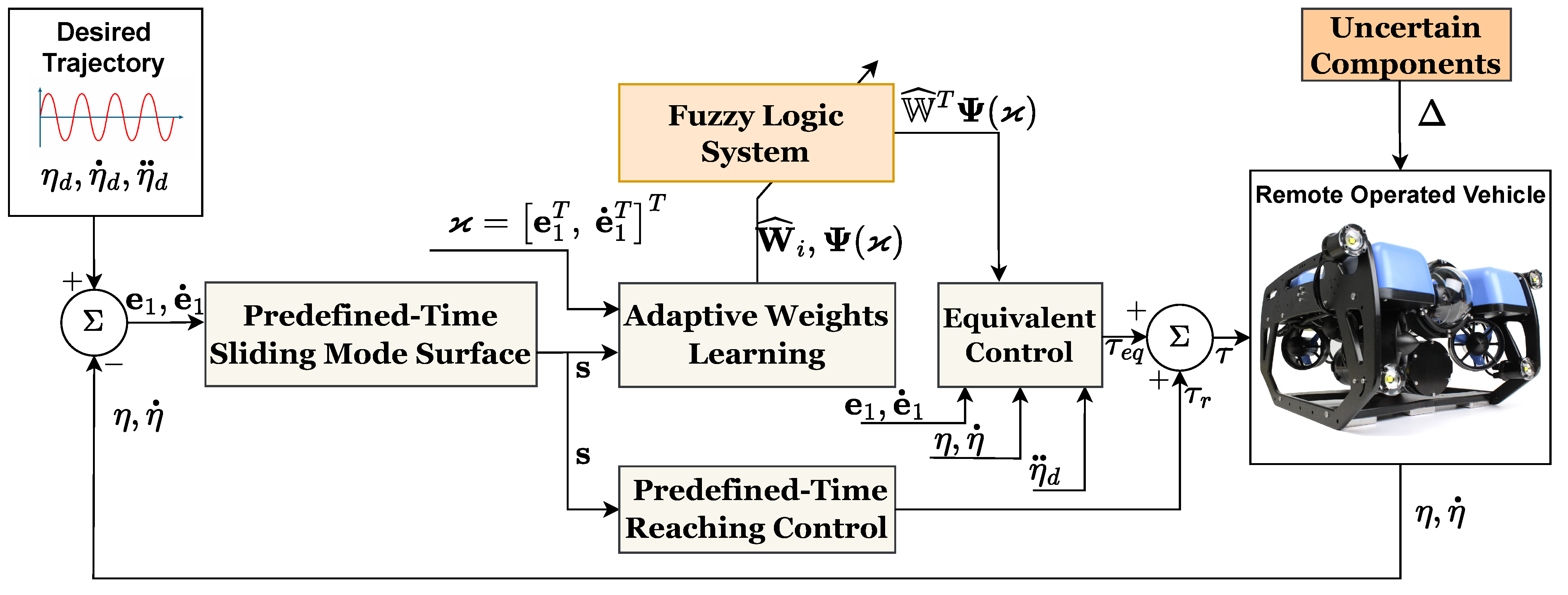
4. Synthesis of Control Design

This section presents a predefined-time control method designed to estimate system convergence in relation to predefined parameters, ensuring predefined-time performance that encompasses both convergence and stability for ROVs in the presence of uncertain factors. An analysis of the stability and convergence characteristics of this method is also included.

4.1. Formulation of Sliding Mode Surface

The Earth-fixed coordinate errors are defined as follows:

$${\mathbf{e}}_1=\mathit{\eta }-{\mathit{\eta }}_d,$$

(15)

where ${\mathbf{e}}_1={[e_{1i},\dots ,e_{1n}]}^T\in {\mathbb{R}}^{n\times 1}$, and ${\mathit{\eta }}_d\in {\mathbb{R}}^{6\times 1}$ denotes the reference Earth-fixed coordinate.

Based on Equation (15), its first and second derivatives with respect to time are given by

$$\begin{array}{c}\hfill \left\{\begin{array}{cc}\hfill {\dot{\mathbf{e}}}_1& =\dot{\mathit{\eta }}-{\dot{\mathit{\eta }}}_d,\hfill \\ \hfill {\ddot{\mathbf{e}}}_1& =\dot{\mathit{J}}\left(\mathit{\eta }\right)\mathit{v}+\mathbf{\Xi }\left(\mathit{\tau }-{\mathit{C}}_o\left(\mathit{v}\right)\mathit{v}-{\mathit{D}}_o\left({\mathit{v}}_r\right)-\mathbf{\Delta }(\mathit{v},\dot{\mathit{v}},{\mathit{v}}_c,{\dot{\mathit{v}}}_c)\right)-{\ddot{\mathit{\eta }}}_d.\hfill \end{array}\right.\end{array}$$

(16)

Based on the proposal in Lemma 1, the sliding mode (SM) surface is formulated as follows:

$$\mathbf{s}={\dot{\mathbf{e}}}_1+{\displaystyle \frac{\pi \Im }{T_{cs}}}\left({\sigma }_{11}{\mathbf{e}}_1+{\sigma }_{21}{\left[{\mathbf{e}}_1\right]}^{2-\alpha }+{\sigma }_{31}{\left[{\mathbf{e}}_1\right]}^{\alpha }\right),$$

(17)

where ${\sigma }_{11}={\sigma }_1$, ${\sigma }_{21}={\displaystyle \frac{{\sigma }_2}{n^{\frac{\alpha -1}{2}}}}$, and ${\sigma }_{31}={\sigma }_3$. The terms ${\sigma }_1,{\sigma }_2,{\sigma }_3$, and ℑ are defined as in Lemma 1. Here, $T_{cs}>0$, and $\mathbf{s}={[s_i,\dots ,s_n]}^T\in {\mathbb{R}}^{n\times 1}$.

Upon reaching the SM surface defined by Equation (17), we have $s_i=0$. Therefore, Equation (17) can be expressed as follows:

$${\dot{\mathbf{e}}}_{1i}=-{\displaystyle \frac{\pi \Im }{T_{cs}}}\left({\sigma }_{11}{\mathbf{e}}_1+{\sigma }_{21}{\left[{\mathbf{e}}_1\right]}^{2-\alpha }+{\sigma }_{31}{\left[{\mathbf{e}}_1\right]}^{\alpha }\right).$$

(18)

Taking the derivative of Equation (17) with respect to time yields

$$\dot{\mathbf{s}}={\ddot{\mathbf{e}}}_1+\mathbf{P}({\mathbf{e}}_1,{\dot{\mathbf{e}}}_1)+\mathbf{Q}({\mathbf{e}}_1,{\dot{\mathbf{e}}}_1),$$

(19)

where $\mathbf{P}({\mathbf{e}}_1,{\dot{\mathbf{e}}}_1)={\displaystyle \frac{\pi \Im }{T_{cs}}}\left({\sigma }_{11}{\dot{\mathbf{e}}}_1+{\sigma }_{21}(2-\alpha ){|{\mathbf{e}}_1|}^{1-\alpha }{\dot{\mathbf{e}}}_1\right)$ and $\mathbf{Q}({\mathbf{e}}_1,{\dot{\mathbf{e}}}_1)={\displaystyle \frac{\pi \Im }{T_{cs}}}{\sigma }_{31}\alpha {|{\mathbf{e}}_1|}^{\alpha -1}{\dot{\mathbf{e}}}_1$.

While incorporating Equation (16), Equation (19) yields

$$\begin{array}{cc}\hfill \dot{\mathbf{s}}& =\dot{\mathit{J}}\left(\mathit{\eta }\right)\mathit{v}+\mathbf{\Xi }\left(\mathit{\tau }-{\mathit{C}}_o\left(\mathit{v}\right)\mathit{v}-{\mathit{D}}_o\left({\mathit{v}}_r\right)-\mathbf{\Delta }(\mathit{v},\dot{\mathit{v}},{\mathit{v}}_c,{\dot{\mathit{v}}}_c)\right)-{\ddot{\mathit{\eta }}}_d+\mathbf{Q}({\mathbf{e}}_1,{\dot{\mathbf{e}}}_1)+\mathbf{P}({\mathbf{e}}_1,{\dot{\mathbf{e}}}_1)\hfill \end{array}.$$

(20)

Theorem 1.

The designed SM surface in Equation (17) guarantees predefined-time convergence of the Earth-fixed coordinate errors within a specified time $T_{cs}$.

Proof. 

Constructing a positive Lyapunov function as follows:

$$V_1={\mathbf{e}}_1^T{\mathbf{e}}_1.$$

(21)

Taking the derivative of Equation (21) while using Equation (18), we obtain

$$\begin{array}{cc}\hfill {\dot{V}}_1& =2{\mathbf{e}}_1{\dot{\mathbf{e}}}_1\hfill \\ \hfill & =-{\displaystyle \frac{2\pi \Im }{T_{cs}}}\left({\sigma }_{11}{\displaystyle \sum _{i=1}^n}{e}_{1i}^2+{\sigma }_{21}{\displaystyle \sum _{i=1}^n}|e_{1i}{|}^{3-\alpha }+{\sigma }_{31}{\displaystyle \sum _{i=1}^n}{|e_{1i}|}^{1+\alpha }\right)\hfill \\ \hfill & \le -{\displaystyle \frac{2\pi \Im }{T_{cs}}}\left({\sigma }_1{\left({\displaystyle \sum _{i=1}^n}{e}_{1i}\right)}^2+{\sigma }_2{\left({\left({\displaystyle \sum _{i=1}^n}{e}_{1i}\right)}^2\right)}^{{\displaystyle \frac{3-\alpha }{2}}}+{\sigma }_3{\left({\left({\displaystyle \sum _{i=1}^n}{e}_{1i}\right)}^2\right)}^{{\displaystyle \frac{1+\alpha }{2}}}\right)\hfill \\ \hfill & \le -{\displaystyle \frac{2\pi \Im }{T_{cs}}}\left({\sigma }_1{V}_1+{\sigma }_2{V}_1^{{\displaystyle \frac{3-\alpha }{2}}}+{\sigma }_3{V}_1^{{\displaystyle \frac{1+\alpha }{2}}}\right)\hfill \end{array}.$$

(22)

Referring to Lemma 1, it is guaranteed that the tracking error $e_{1i}=0$ will be achieved within a predetermined time interval denoted as $T_{cs}$.    □

4.2. FLS Approximation

Examining Equation (20), we observe the term $|{\mathbf{e}}_1{|}^{\alpha -1}{\dot{\mathbf{e}}}_1$ in $\mathbf{Q}({\mathbf{e}}_1,{\dot{\mathbf{e}}}_1)$, which can become unbounded if $e_{1i}=0$ and ${\dot{e}}_{1i}\ne 0$, leading to a singularity issue in the control input. This singularity complicates real-world applications. Additionally, the dependency on the term $\mathbf{\Delta }$ poses challenges for control design. To address this, we express the sum $\mathbf{\Xi }\mathbf{\Delta }+\mathbf{Q}({\mathbf{e}}_1,{\dot{\mathbf{e}}}_1)$ as an AFLS. The FLS is described as follows:

An FLS [39] employs a collection of rules known as IF-THEN rules to establish a relationship between a set of input variables, denoted by $\mathit{\varkappa }={({\varkappa }_i,\dots ,{\varkappa }_n)}^T\in {\mathbb{R}}^n$, and an output variable $z\in \mathbb{R}$. Each rule, indexed by j, takes the following form:

Rule j: If ${\varkappa }_1$ is $R_1^j$ and … and ${\varkappa }_n$ is $R_n^j$ then z is $Q^j$,

• where $R_1^j$, $R_2^j$, …, $R_n^j$ and $Q^j$ represent fuzzy sets. The fuzzy output, when utilizing a singleton fuzzifier, is determined as follows:

$$z={\displaystyle \frac{{\sum }_{j=1}^k{\mathrm{w}}_j\left({\prod }_{i=1}^n{\Phi }_{R_i^j}\left({\varkappa }_i\right)\right)}{{\sum }_{j=1}^k\left({\prod }_{i=1}^n{\Phi }_{R_i^j}\left({\varkappa }_j\right)\right)}}={\mathbf{W}}^T\mathbf{\Psi }\left(\mathit{\varkappa }\right),$$

(23)

where k is the total number of rules employed. Here, ${\Phi }_{R_i^j}\left({\varkappa }_i\right)$ represents the membership function of the $i\mathrm{th}$ input variable ${\varkappa }_i$. For $j=1,\dots ,k$, the vector $\mathbf{W}={[{\mathrm{w}}_j,\dots ,{\mathrm{w}}_k]}^T$ comprises weight components that require adjustment during training. Additionally, $\mathbf{\Psi }\left(\mathit{\varkappa }\right)={[g_j\left(\mathit{\varkappa }\right),\dots ,g_k\left(\mathit{\varkappa }\right)]}^T$ denotes a fuzzy basis vector, where each element $g_j\left(\mathit{\varkappa }\right)$ is expressed as follows:

$$g_j\left(\mathrm{u}\right)={\displaystyle \frac{{\prod }_{i=1}^n{\Phi }_{R_i^j}\left({\varkappa }_i\right)}{{\sum }_{j=1}^k\left({\prod }_{i=1}^n{\Phi }_{R_i^j}\left({\varkappa }_i\right)\right)}}.$$

(24)

Lemma 2

([40]). Suppose there is a continuous function $f\left(\mathit{\varkappa }\right)$ defined on a compact set ${\rm Y}\subset {\mathbb{R}}^{n\times 1}$. It is possible to approximate this function $f\left(\mathit{\varkappa }\right)$ using an FLS, denoted as ${\mathbf{W}}^T\mathbf{\Psi }\left(\mathit{\varkappa }\right)$, such that

$$\underset{\mathbf{u}\in {\rm Y}}{sup}\left|f\left(\mathit{\varkappa }\right)-{\mathbf{W}}^T\mathbf{\Psi }\left(\mathit{\varkappa }\right)\right|\le \phi .$$

(25)

Here, φ is a positive constant. The basis function vector $\mathbf{\Psi }\left(\mathit{\varkappa }\right)$ is defined as $\mathbf{\Psi }\left(\mathit{\varkappa }\right)={[g_j\left(\mathit{\varkappa }\right),\dots ,g_k\left(\mathit{\varkappa }\right)]}^T{\displaystyle \frac{1}{{\sum }_{j=1}^k{g}_j\left(\mathit{\varkappa }\right)}}$, where $\mathbf{W}={[{\mathrm{w}}_j,\dots ,{\mathrm{w}}_k]}^T$ is the ideal constant weight vector, with $k>1$. Each $g_j\left(\mathit{\varkappa }\right)$ is selected as Gaussian functions with the form $g_j\left(\mathit{\varkappa }\right)=exp\left({\displaystyle \frac{-{(\mathit{\varkappa }-{\mathbf{\nu }}_j)}^T(\mathit{\varkappa }-{\mathbf{\nu }}_j)}{{\varsigma }_j^2}}\right)$. Here, ${\varsigma }_j$ denotes the width of the Gaussian function, and ${\mathbf{\nu }}_j={[{\nu }_{ji},\dots ,{\nu }_{jn}]}^T$ represents the center vector.

According to the mentioned FLS’s properties, we can infer that $\parallel \mathbf{\Psi }\left(\mathit{\varkappa }\right)\parallel \le \sqrt{k}$.

Based on the described FLS, the sum $\mathbf{\Xi }\mathbf{\Delta }+\mathbf{Q}({\mathbf{e}}_1,{\dot{\mathbf{e}}}_1)$ is represented as ${\mathbb{W}}^T\mathbf{\Psi }\left(\mathit{\varkappa }\right)+\mathit{\phi }$, where $\mathbb{W}=[{\mathbf{W}}_i,\dots ,{\mathbf{W}}_n]\in {\mathbb{R}}^{k\times n}$ and $\mathit{\phi }=[{\phi }_i,\dots ,{\phi }_n]\in {\mathbb{R}}^{n\times 1}$. Thus, Equation (20) simplifies to

$$\begin{array}{cc}\hfill \dot{\mathbf{s}}& =\dot{\mathit{J}}\left(\mathit{\eta }\right)\mathit{v}+{\mathbb{W}}^T\mathbf{\Psi }\left(\mathit{\varkappa }\right)+\mathit{\phi }+\mathbf{\Xi }\left(\mathit{\tau }-{\mathit{C}}_o\left(\mathit{v}\right)\mathit{v}-{\mathit{D}}_o\left({\mathit{v}}_r\right)\right)-{\ddot{\mathit{\eta }}}_d+\mathbf{P}({\mathbf{e}}_1,{\dot{\mathbf{e}}}_1).\hfill \end{array}$$

(26)

4.3. Formulation of Controller and Its Stability Proof

Drawing upon Equation (26), we formulate the controller as follows:

$$\begin{array}{cc}\hfill \mathit{\tau }& =\mathbf{\Xi }({\mathit{\tau }}_{eq}-{\mathit{\tau }}_r),\hspace{1em}\hspace{1em}\hspace{1em}\hspace{1em}\hspace{1em}\hspace{1em}\hspace{1em}\hspace{1em}\hspace{1em}\hspace{1em}\hspace{1em}\hspace{1em}\hspace{1em}\hspace{1em}\hspace{1em}\hspace{1em}\hspace{1em}\hspace{1em}\hfill \end{array}$$

(27a)

$$\begin{array}{cc}\hfill {\mathit{\tau }}_{eq}& ={\mathit{C}}_o\left(\mathit{v}\right)\mathit{v}+{\mathit{D}}_o\left({\mathit{v}}_r\right)+{\mathbf{\Xi }}^{-1}\left({\ddot{\mathit{\eta }}}_d-\dot{\mathit{J}}\left(\mathit{\eta }\right)\mathit{v}-{\widehat{\mathbb{W}}}^T\mathbf{\Psi }\left(\mathit{\varkappa }\right)-\mathbf{P}({\mathbf{e}}_1,{\dot{\mathbf{e}}}_1)\right),\hfill \end{array}$$

(27b)

$$\begin{array}{cc}\hfill {\mathit{\tau }}_r& ={\displaystyle \frac{\pi \Im }{T_{cr}}}\left({\sigma }_{12}\mathbf{s}+{\sigma }_{22}{\left[\mathbf{s}\right]}^{2-\alpha }+{\sigma }_{32}{\left[\mathbf{s}\right]}^{\alpha }\right)+(\overline{\mathit{\phi }}+\mathit{\chi })\mathrm{sign}\left(\mathbf{s}\right).\hspace{1em}\hspace{1em}\hspace{1em}\hfill \end{array}$$

(27c)

where ${\sigma }_{12}={\sigma }_1$, ${\sigma }_{22}={\displaystyle \frac{{\sigma }_2}{n^{\frac{\alpha -1}{2}}}}$, ${\sigma }_{32}={\sigma }_3$, ${\overline{\phi }}_i>0$, and ${\chi }_i>0$. The terms ${\sigma }_1,{\sigma }_2,{\sigma }_3$, and ℑ are defined as in Lemma 1.

Let the adaptive rule be given by ${\dot{\widehat{\mathbf{W}}}}_i=-{\gamma }_i{s}_i\mathbf{\Psi }\left(\mathit{\varkappa }\right)$, where ${\gamma }_i>0$.

Remark 2.

The use of switching signals, such as $(\overline{\mathit{\phi }}+\mathit{\chi })\mathrm{sign}\left(\mathbf{s}\right)$, may induce undesirable chattering, which could potentially affect the system’s stability and actuator performance. To mitigate this, we have employed a continuous AFLS to approximate and compensate for the system’s uncertainties, including dynamic uncertainties and external disturbances. As a result, the discontinuous control component is only used to compensate for the residual approximation error of the AFLS. This allows the sliding gain to remain sufficiently small, effectively reducing the chattering effect while preserving robust control performance.

Remark 3.

Although the proposed control scheme employs fuzzy approximators, adaptive learning rules, and nonlinear gain structures to enhance robustness and tracking performance, it is recognized that these features introduce additional computational complexity. However, with the recent advancements in embedded hardware technologies—such as high-performance microcontrollers, DSPs, and embedded GPUs—the real-time implementation of such intelligent control strategies has become feasible. Platforms like the NVIDIA Jetson series, STM32 microcontrollers with FPU support, and TI C2000 processors provide sufficient computational resources to support the real-time operation of the proposed method, even under the hardware constraints typically encountered in underwater vehicles.

The control design overview is briefly described in Figure 2.

Theorem 2.

For the ROV dynamic model (10) with uncertain components, if the SM manifold is defined as Equation (17), the control law is given by Equation (27), and the updating law is properly designed, then all signals of the control system are bounded.

Proof. 

Applying the control input (27) to Equation (26), we achieve

$$\dot{\mathbf{s}}={\tilde{\mathbb{W}}}^T\mathbf{\Psi }\left(\mathit{\varkappa }\right)+\mathit{\phi }-{\mathit{\tau }}_r.$$

(28)

The Lyapunov function $V_2={\mathbf{s}}^T\mathbf{s}+{\displaystyle \sum _{i=1}^n}{\tilde{\mathbf{W}}}_i^T{\gamma }_i^{-1}{\tilde{\mathbf{W}}}_i$ is utilized with ${\tilde{\mathbf{W}}}_i={\mathbf{W}}_i-{\widehat{\mathbf{W}}}_i$, where ${\tilde{\mathbf{W}}}_i$ is the $i$th estimation error matrix of the weight. The time derivative of the Lyapunov function is expressed as follows:

$${\dot{V}}_2=2{\mathbf{s}}^T\dot{\mathbf{s}}+2{\displaystyle \sum _{i=1}^n}{\tilde{\mathbf{W}}}_i^T{\gamma }_i^{-1}{\dot{\widehat{\mathbf{W}}}}_i,$$

(29)

where $\dot{\mathbf{s}}={\tilde{\mathbb{W}}}^T\mathbf{\Psi }\left(\mathit{\varkappa }\right)+\mathit{\phi }-{\mathit{\tau }}_r$ and $\tilde{\mathbb{W}}=\mathbb{W}-\widehat{\mathbb{W}}$. Therefore,

$$\begin{array}{cc}\hfill {\dot{V}}_2& =2{\mathbf{s}}^T\left({\tilde{\mathbb{W}}}^T\mathbf{\Psi }\left(\mathit{\varkappa }\right)+\mathit{\phi }-{\mathit{\tau }}_r\right)+2{\displaystyle \sum _{i=1}^n}{\tilde{\mathbf{W}}}_i^T{\gamma }_i^{-1}{\dot{\widehat{\mathbf{W}}}}_i\hfill \\ \hfill & =2{\mathbf{s}}^T\left({\tilde{\mathbb{W}}}^T\mathbf{\Psi }\left(\mathit{\varkappa }\right)+\mathit{\phi }-(\overline{\mathit{\phi }}+\mathit{\chi })\mathrm{sign}\left(\mathbf{s}\right)\right)-{\displaystyle \frac{2\pi \Im }{T_{cr}}}\left({\sigma }_{12}{\displaystyle \sum _{i=1}^n}{s}_i^2+{\sigma }_{22}{\displaystyle \sum _{i=1}^n}|s_i{|}^{3-\alpha }+{\sigma }_{32}{\displaystyle \sum _{i=1}^n}{|s_i|}^{1+\alpha }\right)\hfill \\ \hfill & +2{\displaystyle \sum _{i=1}^n}{\tilde{\mathbf{W}}}_i^T{\gamma }_i^{-1}{\dot{\widehat{\mathbf{W}}}}_i\hfill \\ \hfill & \le -2\mathit{\chi }\parallel \mathbf{s}\parallel -{\displaystyle \frac{2\pi \Im }{T_{cr}}}\left({\sigma }_1{\left({\displaystyle \sum _{i=1}^n}{s}_i\right)}^2+{\sigma }_2{\left({\left({\displaystyle \sum _{i=1}^n}{s}_i\right)}^2\right)}^{{\displaystyle \frac{3-\alpha }{2}}}+{\sigma }_3{\left({\left({\displaystyle \sum _{i=1}^n}{s}_i\right)}^2\right)}^{{\displaystyle \frac{1+\alpha }{2}}}\right)\hfill \\ \hfill & +2{\displaystyle \sum _{i=1}^n}{\tilde{\mathbf{W}}}_i^T\left({\displaystyle \frac{1}{\gamma }}{\dot{\widehat{\mathbf{W}}}}_i+s_i\mathbf{\Psi }\left(\mathit{\varkappa }\right)\right)\hfill \end{array}.$$

(30)

With the designed adaptive rule, Equation (30) becomes

$$\begin{array}{cc}\hfill {\dot{V}}_2& \le -2\mathit{\chi }\parallel \mathbf{s}\parallel -{\displaystyle \frac{2\pi \Im }{T_{cr}}}\left({\sigma }_1{\left({\displaystyle \sum _{i=1}^n}{s}_i\right)}^2+{\sigma }_2{\left({\left({\displaystyle \sum _{i=1}^n}{s}_i\right)}^2\right)}^{{\displaystyle \frac{3-\alpha }{2}}}+{\sigma }_3{\left({\left({\displaystyle \sum _{i=1}^n}{s}_i\right)}^2\right)}^{{\displaystyle \frac{1+\alpha }{2}}}\right)\hfill \\ \hfill & \le 0.\hfill \end{array}$$

(31)

Inequality (31) indicates that both $\mathbf{s}$ and $\tilde{\mathbb{W}}$ are bounded. From Equation (17), it follows that both ${\mathbf{e}}_1$ and ${\dot{\mathbf{e}}}_1$ are also bounded. The boundedness of $\mathit{\eta }$ and $\dot{\mathit{\eta }}$ can be inferred from the boundedness of ${\mathit{\eta }}_d$ and ${\dot{\mathit{\eta }}}_d$. Consequently, all signals in Equation (28) are bounded, ensuring that $\dot{\mathbf{s}}$ is bounded as well. Thus, all signals in the control system are bounded. However, it is not essential for the sliding mode manifold $\mathbf{s}$ to approach zero within a predefined time. Therefore, we present the next theorem to ensure that the sliding mode manifold $\mathbf{s}$ converges to zero within the specified time frame.

Theorem 3.

For the dynamic model described in Equation (26), which includes the modeling error $\mathit{\phi }$ and the approximation error ${\tilde{\mathbb{W}}}^T\mathbf{\Psi }\left(\mathit{\varkappa }\right)$, applying the control law presented in Equation (27) while selecting the design parameter ${\chi }_i$ in Equation (27c) such that $\parallel {\tilde{\mathbb{W}}}^T{\mathbf{\Psi }\left(\mathit{\varkappa }\right)\parallel }_F\le {\chi }_i$ ensures that both $\mathbf{s}$ and ${\mathbf{e}}_1$ achieve predetermined-time convergence and stability.

The proposed formulation defines $\Lambda$ as follows:

$$\Lambda =2\mathit{\chi }\parallel \mathbf{s}\parallel +{\displaystyle \frac{2\pi \Im }{T_{cr}}}\left({\sigma }_1{\left({\displaystyle \sum _{i=1}^n}{s}_i\right)}^2+{\sigma }_2{\left({\left({\displaystyle \sum _{i=1}^n}{s}_i\right)}^2\right)}^{{\displaystyle \frac{3-\alpha }{2}}}+{\sigma }_3{\left({\left({\displaystyle \sum _{i=1}^n}{s}_i\right)}^2\right)}^{{\displaystyle \frac{1+\alpha }{2}}}\right)\le -{\dot{V}}_2.$$

Integrating $\Lambda$ over time yields the following inequality:

$${\displaystyle \underset{0}{\overset{t}{\int }}}\Lambda \left(t\right)dt\le V_2\left(0\right)-V_2\left(t\right)=V_2(\mathbf{s}\left(0\right),\tilde{\mathbf{W}})-V_2(\mathbf{s}\left(t\right),\tilde{\mathbf{W}}).$$

(32)

Here, $V_2(\mathbf{s}\left(0\right),\tilde{\mathbf{W}})$ represents the initial value of $V_2$, and $V_2(\mathbf{s}\left(t\right),\tilde{\mathbf{W}})$ is its value at time t.

As $V_2(\mathbf{s}\left(t\right),\tilde{\mathbf{W}})$ remains both bounded and continuously decreasing, it guarantees that $\mathbf{s}$ and each ${\tilde{\mathbf{W}}}_i$ ($i=1,\dots ,n$) do not diverge over time.

Furthermore, since $\mathbf{s}$ depends on both ${\mathbf{e}}_1$ and ${\dot{\mathbf{e}}}_1$, its boundedness directly ensures that the trajectory tracking error remains constrained.

To establish the predefined-time stability of the system, we define a Lyapunov function as $V_3={\mathbf{s}}^T\mathbf{s}$. Differentiating this function with respect to time yields

$$\begin{array}{cc}\hfill {\dot{V}}_3& =2{\mathbf{s}}^T\left({\tilde{\mathbb{W}}}^T\mathbf{\Psi }\left(\mathit{\varkappa }\right)+\mathit{\phi }-(\overline{\mathit{\phi }}+\mathit{\chi })\mathrm{sign}\left(\mathbf{s}\right)\right)-{\displaystyle \frac{2\pi \Im }{T_{cr}}}\left({\sigma }_{12}{\displaystyle \sum _{i=1}^n}{s}_i^2+{\sigma }_{22}{\displaystyle \sum _{i=1}^n}|s_i{|}^{3-\alpha }+{\sigma }_{32}{\displaystyle \sum _{i=1}^n}{|s_i|}^{1+\alpha }\right).\hfill \end{array}$$

(33)

Simplifying, we have

$$\begin{array}{cc}\hfill {\dot{V}}_3& \le 2{\mathbf{s}}^T{\tilde{\mathbb{W}}}^T\mathbf{\Psi }\left(\mathit{\varkappa }\right)-2\mathit{\chi }\parallel \mathbf{s}\parallel -{\displaystyle \frac{2\pi \Im }{T_{cr}}}\left({\sigma }_1{\left({\displaystyle \sum _{i=1}^n}{s}_i\right)}^2+{\sigma }_2{\left({\left({\displaystyle \sum _{i=1}^n}{s}_i\right)}^2\right)}^{{\displaystyle \frac{3-\alpha }{2}}}+{\sigma }_3{\left({\left({\displaystyle \sum _{i=1}^n}{s}_i\right)}^2\right)}^{{\displaystyle \frac{1+\alpha }{2}}}\right),\hfill \end{array}$$

(34)

which further simplifies to

$${\dot{V}}_3\le -{\displaystyle \frac{2\pi \Im }{T_{cr}}}\left({\sigma }_1{V}_3+{\sigma }_2{V}_3^{{\displaystyle \frac{3-\alpha }{2}}}+{\sigma }_3{V}_3^{{\displaystyle \frac{1+\alpha }{2}}}\right).$$

(35)

It is well known that the Gaussian function $g_j\left(\mathit{\varkappa }\right)$ is constrained within the range $0<g_j\left(\mathit{\varkappa }\right)\le 1$, thus $\parallel \mathbf{\Psi }\left(\mathit{\varkappa }\right)\parallel \le \sqrt{k}$.

Using the properties of the Frobenius norm,

$${∥{\tilde{\mathbb{W}}}^T\mathbf{\Psi }\left(\mathit{\varkappa }\right)∥}_F\le {∥{\tilde{\mathbb{W}}}^T∥}_F∥\mathbf{\Psi }\left(\mathit{\varkappa }\right)∥.$$

(36)

From Theorem 2 and the above, ${∥{\tilde{\mathbb{W}}}^T\mathbf{\Psi }\left(\mathit{\varkappa }\right)∥}_F$ is bounded. Therefore,

$${\dot{V}}_3\le -{\displaystyle \frac{2\pi \Im }{T_{cr}}}\left({\sigma }_1{V}_3+{\sigma }_2{V}_3^{{\displaystyle \frac{3-\alpha }{2}}}+{\sigma }_3{V}_3^{{\displaystyle \frac{1+\alpha }{2}}}\right).$$

(37)

Referring to Lemma 1, it is ensured that both $\mathbf{s}$ and ${\mathbf{e}}_1$ achieve convergence and stability within the predetermined time $T_{cr}$.    □

5. Simulations

5.1. Configuration of the Testing System

The dynamics of the ROV are shaped by several factors, including the inertia mass and added mass models, Coriolis and centripetal forces, gravitational and buoyancy forces, damping forces, the thruster model, and the Euler transformation model. Each subsystem is represented by detailed simulation models. The ROV’s governing differential equations are solved using the ODE5 function, which implements a fixed-step method with a relative tolerance of 0.001. All simulations were carried out using MATLAB 2021b/SIMULINK, a robust platform for modeling, simulating, and analyzing dynamic systems.

Simulations play a crucial role in evaluating key performance metrics that determine the controller’s efficiency, including convergence rate, tracking accuracy, and robustness. Additionally, they enable a detailed comparison of tracking error accuracy, chattering mitigation, and robustness against uncertainties between the proposed approach (M4) and established methods such as SMC, fixed-time, and predefined-time control. Specifically, the methods in [23,36,41] are denoted as M1, M2, and M3, respectively. This comprehensive analysis highlights the proposed controller’s potential to significantly enhance trajectory tracking in ROVs, providing valuable insights into its advantages over conventional control strategies.

In M1 [36], the SM surface is designed as $\mathbf{s}={\kappa }_{10}{\mathbf{e}}_1+{\dot{\mathbf{e}}}_1$, where ${\kappa }_{10}$ is a positive constant. Accordingly, the control law of M1 is designed as follows:

$$\mathit{\tau }={\mathit{C}}_o\left(\mathit{v}\right)\mathit{v}+{\mathit{D}}_o\left({\mathit{v}}_r\right)+{\mathbf{M}}_o{\mathit{J}}^{-1}\left(\mathit{\eta }\right)\left(-\dot{\mathit{J}}\left(\mathit{\eta }\right)\mathit{v}+{\ddot{\mathit{\eta }}}_d+c{\dot{\mathbf{e}}}_1+{\kappa }_{11}\mathbf{s}+{\kappa }_{12}\mathrm{sign}\left(\mathbf{s}\right)\right)$$

(38)

where ${\kappa }_{11}$ and ${\kappa }_{12}$ are positive constants.

In M2 [41], the SM surface is designed as $\mathbf{s}={\mathbf{e}}_1+{\displaystyle \frac{1}{{\omega }_2}}|{\mathbf{e}}_1{|}^{p_{21}}\mathrm{sign}\left({\mathbf{e}}_1\right)+{\displaystyle \frac{1}{{\beta }_2}}{|{\dot{\mathbf{e}}}_1|}^{q_{21}}\mathrm{sign}\left({\dot{\mathbf{e}}}_1\right)$, where $p_{21}>1$, $0<q_{21}<1$, and ${\kappa }_{21}$, ${\kappa }_{22}$, ${\omega }_2$, and ${\beta }_2$ are positive constants. Accordingly, the control law for M2 is designed as

$$\begin{array}{cc}\hfill \mathit{\tau }=& {\mathit{M}}_o{\mathit{J}}^{-1}\left(\mathit{\eta }\right)(-\dot{\mathit{J}}\left(\mathit{\eta }\right)\mathit{v}+{\displaystyle \frac{{\beta }_2}{q_{21}}}{|{\dot{\mathbf{e}}}_1|}^{1-q_{21}}({\kappa }_{21}\mathbf{s}+{\kappa }_{22}\mathrm{sign}\left(\mathbf{s}\right)\hfill \\ \hfill & +{\dot{\mathbf{e}}}_1+{\displaystyle \frac{p_{21}}{{\omega }_2}}{|{\mathbf{e}}_1|}^{p_{21}-1}{\dot{\mathbf{e}}}_1)+{\ddot{\mathit{\eta }}}_d)+{\mathit{C}}_o\left(\mathit{v}\right)\mathit{v}+{\mathit{D}}_o\left({\mathit{v}}_r\right).\hfill \end{array}$$

(39)

In M3 [23], the SM surface is designed as $\mathbf{s}={\mathbf{e}}_1+{\displaystyle \frac{1}{{\omega }_3}}|{\mathbf{e}}_1{|}^{p_1}\mathrm{sign}\left({\mathbf{e}}_1\right)+{\displaystyle \frac{1}{{\beta }_3}}{|{\dot{\mathbf{e}}}_1|}^{q_1}\mathrm{sign}\left({\dot{\mathbf{e}}}_1\right)$, where $p_1>1$, $0<q_1<1$, $q_2>1$, $0<p_2<1$, and ${\kappa }_{31}$, ${\kappa }_{32}$, ${\omega }_3$, and ${\beta }_3$ are positive constants. Accordingly, the control law of M3 is expressed as follows:

$$\begin{array}{cc}\hfill \mathit{\tau }=& {\mathit{M}}_o{\mathit{J}}^{-1}\left(\mathit{\eta }\right)(-\dot{\mathit{J}}\left(\mathit{\eta }\right)\mathit{v}+{\displaystyle \frac{{\beta }_3}{q_{31}}}{|{\dot{\mathbf{e}}}_1|}^{1-q_{31}}({\displaystyle \frac{C_v}{T_c}}\left({\displaystyle \frac{{\kappa }_{31}}{2^{p_{32}}}}{\mathbf{s}}^{2p_{32}-1}+{\displaystyle \frac{{\kappa }_{32}}{2^{q_{32}}}}{\mathbf{s}}^{2q_{32}-1}\right)\mathrm{sign}\left(\mathbf{s}\right)\hfill \\ \hfill & +{\dot{\mathbf{e}}}_1+{\displaystyle \frac{p_{31}}{{\omega }_3}}{|{\mathbf{e}}_1|}^{p_{31}-1}{\dot{\mathbf{e}}}_1)+{\ddot{\mathit{\eta }}}_d)+{\mathit{C}}_o\left(\mathit{v}\right)\mathit{v}+{\mathit{D}}_o\left({\mathit{v}}_r\right),\hfill \end{array}$$

(40)

where

$$C_v=\left\{\begin{array}{cc}{\displaystyle \frac{1}{{\kappa }_{32}^{\frac{1}{q_{32}}}}\frac{1}{1-q_{32}}{\kappa }_{32}^{\frac{1-q_{32}}{q_{32}}},}\hfill & 0<V\left(x\right)<1\hfill \\ {\displaystyle \frac{1}{{\kappa }_{31}^{\frac{1}{p_{32}}}}\frac{2^{p_{3}2-1}}{1-p_{32}}{\kappa }_{31}^{\frac{1-p_{32}}{p_{32}}},}\hfill & V\left(x\right)>1.\hfill \end{array}\right.$$

To evaluate the controller’s effectiveness on the ROV model, the BlueROV2 platform, as shown in Figure 3 [36], is utilized, with its parameters presented in

Table 2. System parameters for the dynamic modeling of BlueROV2.

Parameter	Value (Units)	Parameter	Value (Units)	Parameter	Value (Units)
m	$11.5$ kg	W	$112.8$ N	B	$114.8$ N
$I_x$	$0.16$ kg·m2	$I_y$	$0.16$ kg·m2	$I_z$	$0.16$ kg·m2
${\mathrm{K}}_{\mathrm{p}}$	$-0.07$ Ns/rad	${\mathrm{M}}_{\mathrm{q}}$	$-0.07$ Ns/rad	${\mathrm{N}}_{\mathrm{r}}$	$-0.07$ Ns/rad
${\dot{\mathrm{K}}}_{\mathrm{p}}$	$-0.12$ kg·m2/rad	${\dot{\mathrm{M}}}_{\mathrm{q}}$	$-0.12$ kg·m2/rad	${\dot{\mathrm{N}}}_{\mathrm{r}}$	$-0.12$ kg·m2/rad
${\mathrm{K}}_{\mathrm{p}}+{\mathrm{K}}_{|\mathrm{p}|\mathrm{p}}|\mathrm{p}|$	$-1.55$ Ns2/rad2	${\mathrm{M}}_{\mathrm{q}}+{\mathrm{M}}_{|\mathrm{q}|\mathrm{q}}|\mathrm{q}|$	$-1.55$ Ns2/rad2	${\mathrm{N}}_{\mathrm{r}}+{\mathrm{N}}_{|\mathrm{r}|\mathrm{r}}|\mathrm{r}|$	$-1.55$ Ns2/rad2
${\mathrm{X}}_{\mathrm{u}}$	$-4.03$ Ns/m	${\mathrm{Y}}_{\mathrm{v}}$	$-6.22$ Ns/m	${\mathrm{Z}}_{\mathrm{w}}$	$-5.18$ Ns/m
${\dot{\mathrm{X}}}_{\mathrm{u}}$	$-5.5$ kg	${\dot{\mathrm{Y}}}_{\mathrm{v}}$	$-12.7$ kg	${\dot{\mathrm{Z}}}_{\mathrm{w}}$	$-14.57$ kg
${\mathrm{X}}_{\mathrm{u}}+{\mathrm{X}}_{|\mathrm{u}|\mathrm{u}}|\mathrm{u}|$	$-18.18$ Ns2/m2	${\mathrm{Y}}_{\mathrm{v}}+{\mathrm{Y}}_{|\mathrm{v}|\mathrm{v}}|\mathrm{v}|$	$-21.66$ Ns2/m2	${\mathrm{Z}}_{\mathrm{w}}+{\mathrm{Z}}_{|\mathrm{w}|\mathrm{w}}|\mathrm{w}|$	$-36.99$ Ns2/m2

. Additionally, the table includes the added mass and hydrodynamic coefficients.

To maintain consistency across the simulation experiments, all tests were conducted using the same target trajectory for the ROV, as presented in

Table 3. Parameters of the control algorithms and desired trajectory of the ROV.

Control Method	Category	Notation	Value
M1	Parameters	${\kappa }_{10},{\kappa }_{11},{\kappa }_{12}$	$2,2,1.5$
M2	Parameters	${\omega }_2,{\beta }_2,p_{21},q_{21},{\kappa }_{21},{\kappa }_{22}$	$3,3,1.5,0.8,2,1.5$
M3	Parameters	${\omega }_3,{\beta }_3,p_{31},q_{31},{\kappa }_{31},{\kappa }_{32}$	$3,3,1.5,0.8,1,1$
		$p_{32},q_{32}$	$0.9,1.8$
M4	Parameters	${\sigma }_1,{\sigma }_2,{\sigma }_3,\alpha ,{\chi }_i,{\overline{\phi }}_i,{\gamma }_i$	$1,1,1,0.8,0.0005,0.0005,1.6$
	Membership Functions	${\Phi }_{R_i^1},{\Phi }_{R_i^2},{\Phi }_{R_i^3}$	$exp\left[-{\left({\displaystyle \frac{u_i+\frac{\pi }{6}}{\frac{\pi }{24}}}\right)}^2\right],exp\left[-{\left({\displaystyle \frac{u_i+\frac{\pi }{12}}{\frac{\pi }{24}}}\right)}^2\right],exp\left[-{\left({\displaystyle \frac{u_i}{\frac{\pi }{24}}}\right)}^2\right]$
		${\Phi }_{R_i^4},{\Phi }_{R_i^5}$	$exp\left[-{\left({\displaystyle \frac{u_i-\frac{\pi }{12}}{\frac{\pi }{24}}}\right)}^2\right],exp\left[-{\left({\displaystyle \frac{u_i-\frac{\pi }{6}}{\frac{\pi }{24}}}\right)}^2\right]$
–	Desired Trajectory	$x_d,y_d,z_d,{\varphi }_d,{\theta }_d,{\psi }_d$	$5cos\left(0.05t\right)+5,5sin\left(0.05t\right),0.1t,0,0,-{\displaystyle \frac{2\pi }{100}}t$

. For a fair and objective performance comparison, the control parameters for M1–M3 were carefully selected through extensive tuning based on their original designs. The tuning process involved trial-and-error simulations combined with evaluations of convergence speed, steady-state error, and control effort. Furthermore, all tuning was performed under identical simulation settings, using the same ROV system and initial conditions as those applied for the proposed method. The control parameters for all four methods are summarized in Table 3.

In M4, the AFLS processes input signals that include position tracking errors and their derivatives, represented as $\mathit{\varkappa }={\left[{\mathbf{e}}_1^T,{\mathbf{e}}_2^T\right]}^T\in {\mathbb{R}}^{2n\times 1}$. The design employs five symmetric Gaussian membership functions, labeled $j=1$ to $j=5$, with their parameters finely tuned through a systematic trial-and-error optimization process.

Remark 4.

The learning rate ${\gamma }_i$ affects the adaptation speed of the fuzzy weights. A smaller ${\gamma }_i$ yields slower but more stable convergence, while a larger ${\gamma }_i$ accelerates learning at the risk of increased sensitivity to noise and potential chattering. Importantly, ${\gamma }_i$ influences the fuzzy approximator’s learning speed but does not affect the predefined-time stability guarantees established in Theorem 3. For practical tuning, ${\gamma }_i$ should balance adaptation speed and robustness, starting from moderate values and adjusted based on system performance.

To demonstrate predefined-time convergence, stability adaptability, and precision under the proposed strategy, the numerical simulations were conducted to assess various aspects of the control approach. The experiments are organized into two examples, each designed to assess various aspects of the control approach.

Example 1.

The analysis is conducted with the initial states ${\mathit{\eta }}_0=[1,-1,6,0.5,0.5,0.5]$, utilizing various predefined-time parameters as follows: $T_c=4\mathit{s},T_c=5\mathit{s},T_c=6\mathit{s},T_c=7\mathit{s},T_c=8\mathit{s},\mathit{and}{T}_c=9\mathit{s}$. This example focuses on evaluating the predefined-time convergence of the proposed approach. The simulation time is set to $10\mathit{s}$.

Example 2.

The tracking performance of the ROV is evaluated under four different controller configurations, with the predefined-time parameter set to $T_c=5\mathit{s}$ for M3 and M4. The initial states are given as ${\mathit{\eta }}_0=[-1,1,3,0,0,0.4]$, and the simulation time is established at $70\mathit{s}$.

Tracking performance is defined by the ROV’s ability to follow the desired trajectory and is quantitatively assessed by measuring the three-dimensional position error during path tracking. In this analysis, the root-mean-square method (RMSM) quantifies the tracking error, facilitating the comparative evaluation of control methodologies in terms of precision and stability. The RMSM formula is given by $E_{x,y,z,\varphi ,\theta ,\psi }=\sqrt{{\displaystyle \frac{1}{J}}{\sum }_{i=1}^J{\left({\eta }_{di}-{\eta }_i\right)}^2}$, where J is the total number of samples. The root-mean-square errors (RMSEs) for each degree of freedom (DOF) (x, y, z, and $\varphi$, $\theta$, $\psi$) are denoted as $E_x$, $E_y$, $E_z$, $E_{\varphi }$, $E_{\theta }$, and $E_{\psi }$, respectively. In this formula, ${\left[{\eta }_i\right]}^T$ represents the vector of actual values (including positions and orientations) at time index i, while ${\left[{\eta }_{di}\right]}^T$ represents the vector of desired values.

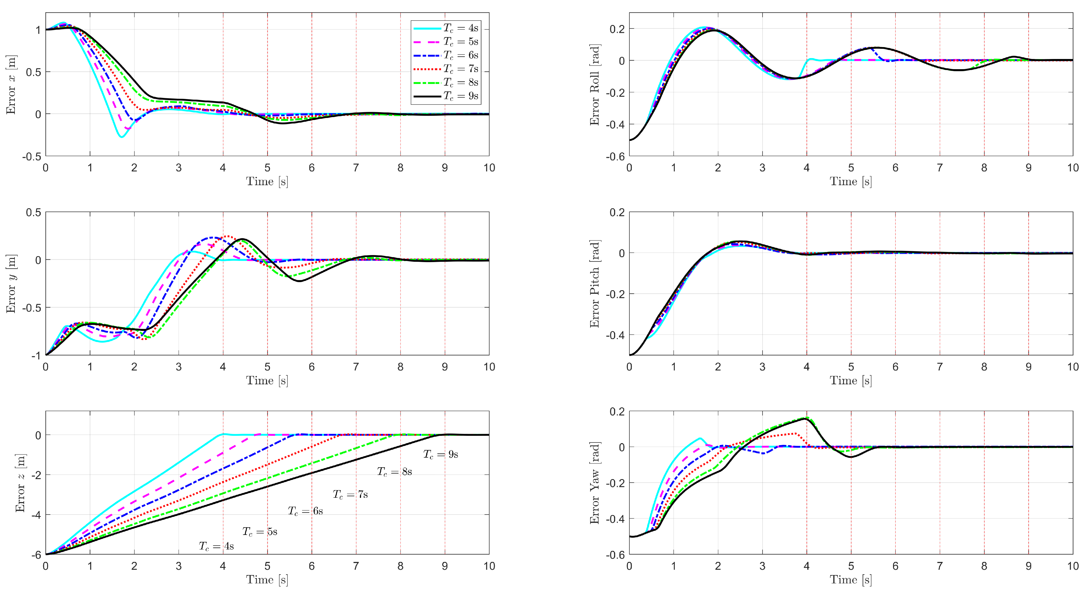
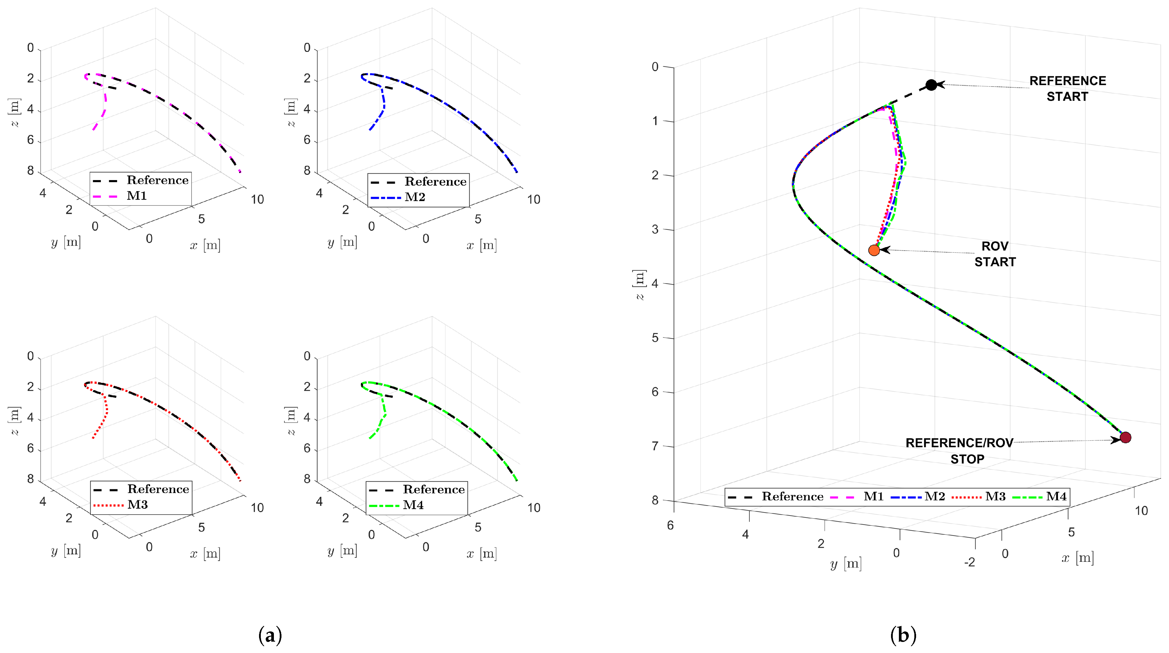
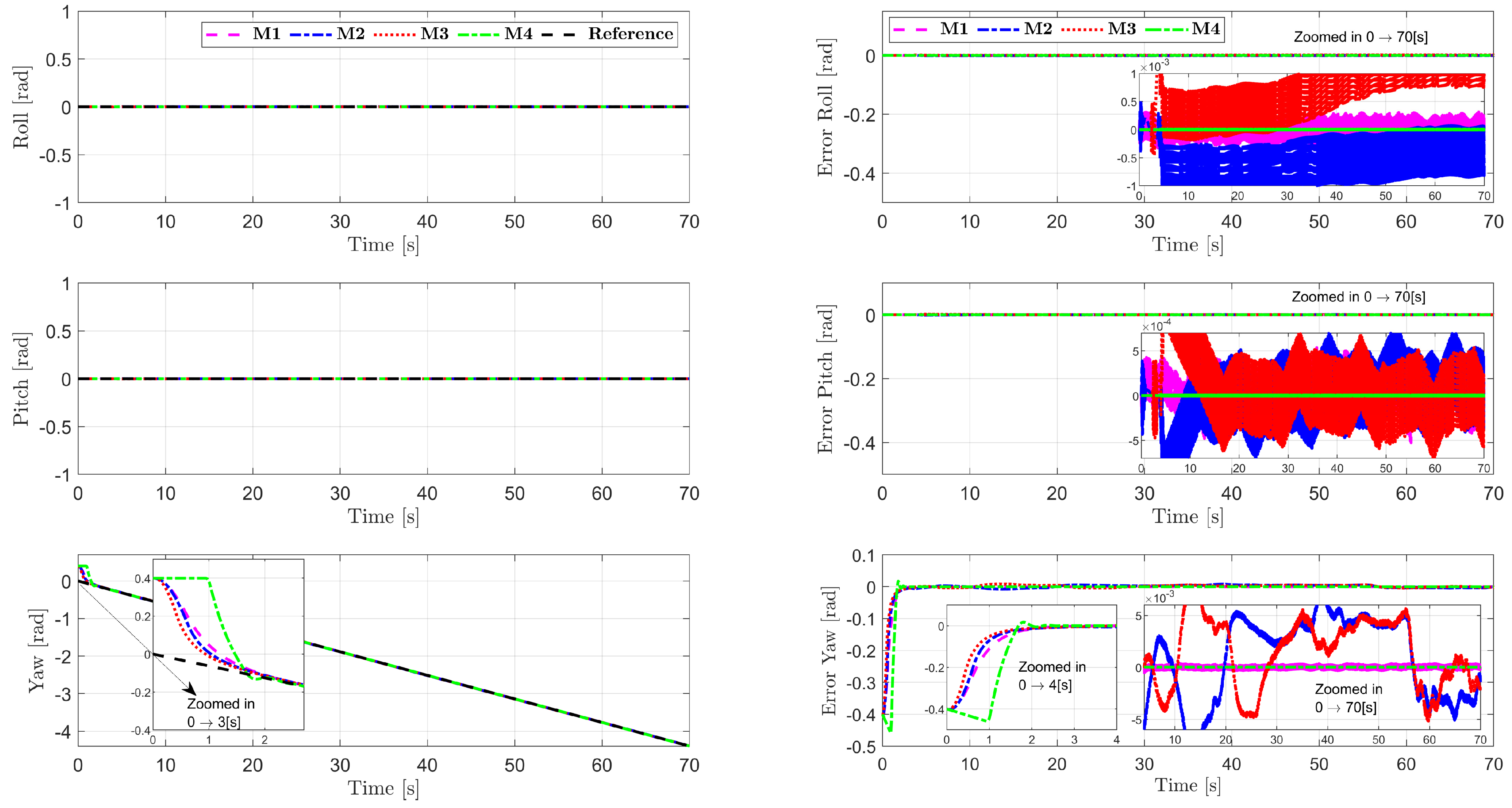
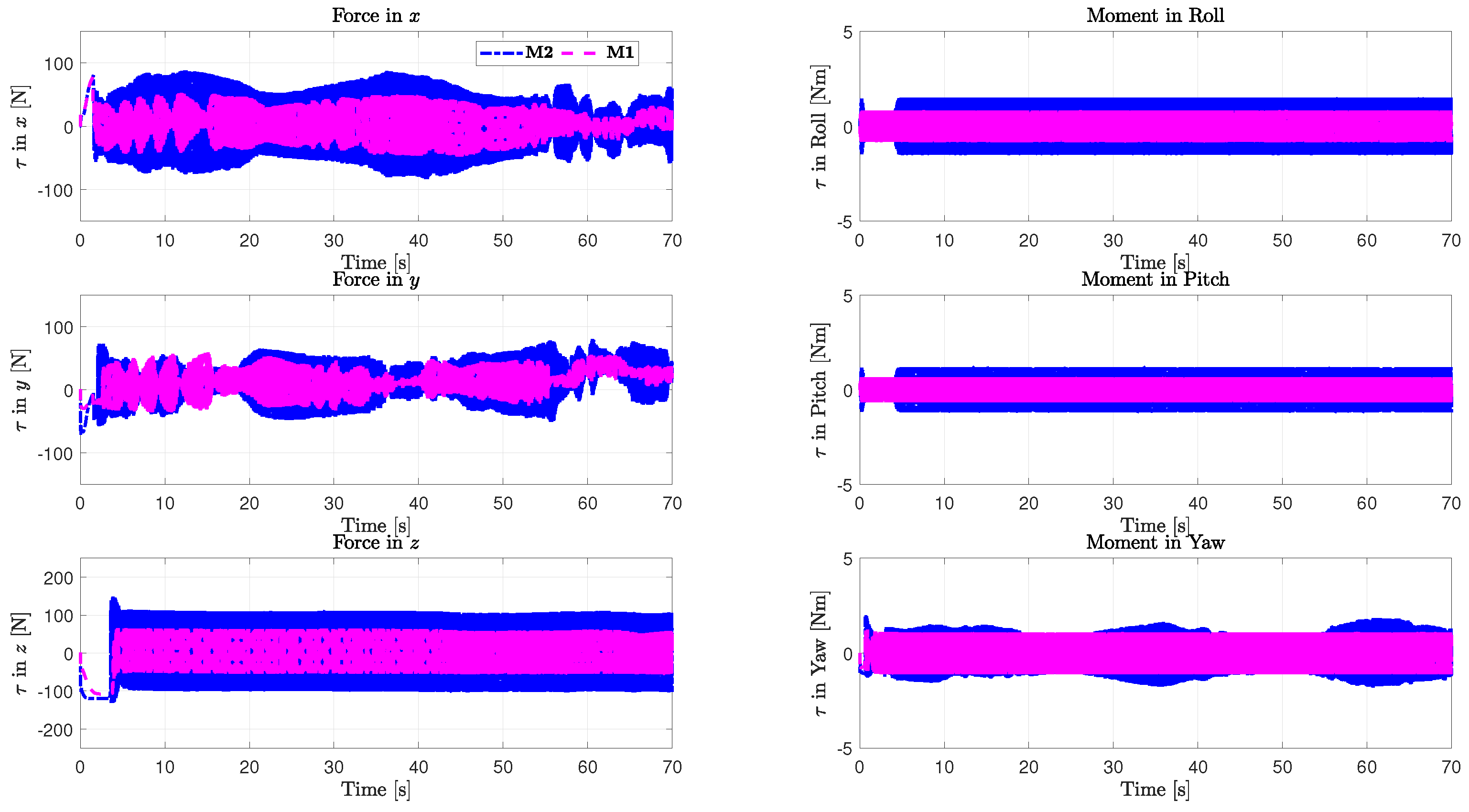
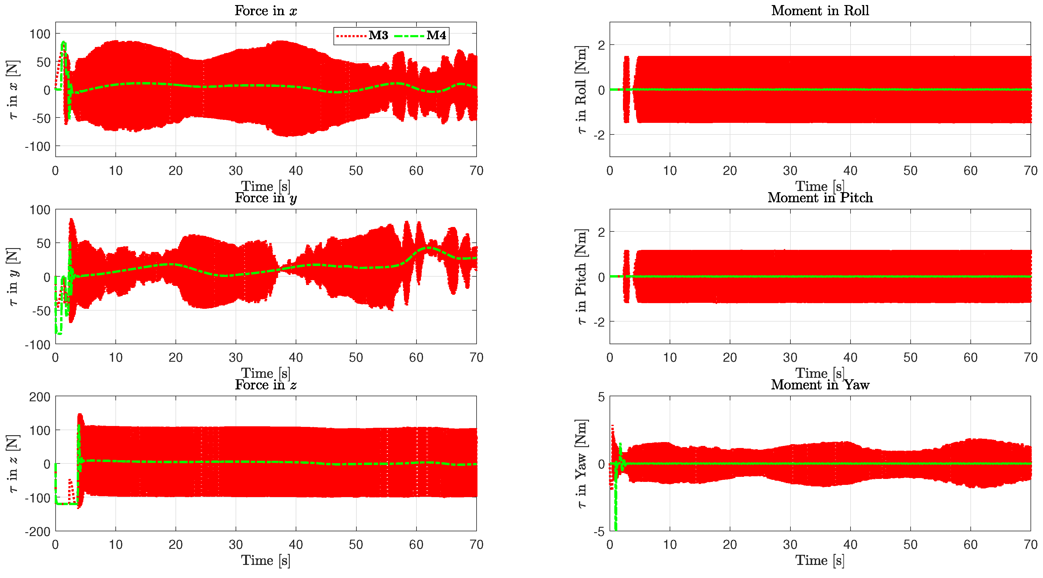
5.2. Analysis of Example 1

By analyzing Figure 4, we observe that the actual convergence time of the ROV at each DOF dynamically varies with the predefined-time parameter $T_c$, and it closely follows the predefined value. For instance, to achieve the desired depth of 6 m along the z-axis at different predefined-time points $T_c$, the proposed controller consistently meets the target. Similarly, for the other joints, the controller achieves the desired position within or near the given time interval $T_c$. In summary, the actual convergence time of the proposed M4 is directly influenced by the predefined-time parameter $T_c$, thereby demonstrating the predefined-time adjustability of M4.

5.3. Analysis of Example 2

The three-dimensional trajectory tracking of the ROV for various DOFs under the influence of the four controllers is illustrated in Figure 5. We observe that all four controllers can effectively manipulate the ROV to achieve the desired trajectory. The comparison of RMSE with the reference trajectory is shown in Figure 6.

Figure 7 presents the comparison of position tracking and position error for each DOF. Additionally, the comparison of orientation tracking and orientation error for each DOF is illustrated in Figure 8.

Firstly, we conduct a comparison between the two predefined-time methods, M4 and M3. We analyze the convergence of states under these two methods and observe that when the predefined-time parameter of M4 is set to $T_c=4\mathrm{s}$, the tracking errors for each DOF of the ROV converge to near zero in approximately 4 s, as shown in Figure 7 and Figure 8. The actual convergence time closely matches the predefined-time parameter $T_c$. Furthermore, after convergence, the system error remains within a very small range, as indicated in Figure 6 and

Table 4. RMSEs via four control algorithms.

Method	${\mathit{E}}_{\mathit{x}}$	${\mathit{E}}_{\mathit{y}}$	${\mathit{E}}_{\mathit{z}}$	${\mathit{E}}_{\mathit{\varphi }}$	${\mathit{E}}_{\mathit{\theta }}$	${\mathit{E}}_{\mathit{\psi }}$
M1	$1.8044\times {10}^{-2}$	$7.157\times {10}^{-3}$	$1.6382\times {10}^{-2}$	$1.768\times {10}^{-4}$	$2.190\times {10}^{-4}$	$1.777\times {10}^{-4}$
M2	$2.0615\times {10}^{-2}$	$8.193\times {10}^{-3}$	$5.789\times {10}^{-3}$	$6.606\times {10}^{-4}$	$3.716\times {10}^{-4}$	$4.1323\times {10}^{-3}$
M3	$2.0732\times {10}^{-2}$	$8.4705\times {10}^{-3}$	$7.021\times {10}^{-3}$	$8.923\times {10}^{-4}$	$4.26\times {10}^{-4}$	$3.6398\times {10}^{-3}$
M4	$1.5701\times {10}^{-2}$	$6.8222\times {10}^{-3}$	$1.1052\times {10}^{-3}$	$4.7\times {10}^{-6}$	$4.5\times {10}^{-6}$	$3.25\times {10}^{-5}$

. These results verify the stability and predefined-time convergence of the proposed M4.

In contrast, M3 does not guarantee convergence within the predefined time $T_c$, particularly for DOF z, where the convergence time is approximately 5 to 6 s. This issue arises from the control design in M3, which ensures predefined-time convergence only during the reaching phase while still employing a fixed-time sliding surface. Consequently, M3 has a longer actual convergence time than the predefined-time parameter.

Next, we compare the simulation results of the four control strategies, as illustrated in Figure 5, Figure 6, Figure 7 and Figure 8 and Table 4.

By examining the simulation outcomes presented in Figure 5, Figure 6, Figure 7 and Figure 8 and Table 4, several key observations can be made. As shown in the zoomed-in sections of Figure 7 and Figure 8, controller M4 ensures system convergence within a predefined time frame for all DOFs. This is attributed to the advantages of the predefined-time sliding surface, the predefined-time reaching law, and the designed FLS. The actual convergence time closely matches the predefined value, enabling precise system tuning.

In this case, M3 does not guarantee convergence within the predefined time $T_c$, particularly for DOF z, where the convergence time is approximately 5 to 6 s, as mentioned above. In general, M1 has the slowest convergence time due to its reliance on a sliding mode approach, resulting in an actual convergence time that exceeds the desired value, especially for DOF z. It requires around 6 s for DOF z to achieve satisfactory tracking performance. M2 demonstrates a better convergence time than M1, but it is still slower than both M3 and M4, requiring around 5 s for DOF z to attain satisfactory tracking performance.

The comparison of RMSE values in Table 4 across the four control methods demonstrates that M4 consistently outperforms the other methods, achieving significant accuracy improvements. Specifically, M4 reduces errors by 12.98% to 24.27% in $E_x$ and 4.68% to 19.46% in $E_y$. More notably, in $E_z$, M4 shows substantial improvements ranging from 80.91% to 93.25%, while for rotational errors $E_{\varphi }$, $E_{\theta }$, and $E_{\psi }$, it achieves remarkable reductions of 97.34% to 99.47%, indicating a significant enhancement in stability and precision.

From the comparison of the tracking trajectories and tracking errors at each DOF in Figure 7 and Figure 8, we observe that M4 not only achieves the desired convergence time but also maintains the smallest tracking errors, as clearly seen in the zoomed-in parts of Figure 7 and Figure 8, which focus on the interval from 4s to 70s. This includes both position and orientation errors throughout the ROV’s operating time. Additionally, M4 demonstrates greater robustness compared to the three remaining methods, as the AFLS effectively estimates the entire range of uncertainties, including dynamic uncertainties and external disturbances. Meanwhile, in an attempt to cope with uncertain components, the other three methods rely on large robust values, which result in significant chattering. These results highlight that M4 is the most effective among the four methods, particularly in minimizing errors in both position and orientation, making it a superior choice for precise control applications.

Figure 9 and Figure 10 show the control inputs, including forces and moments, for the different controllers. Notably, a shorter convergence time is typically associated with higher energy consumption. In particular, for M1, M2, and M3, achieving a shorter convergence time while maintaining satisfactory control performance requires larger robust gains in their control laws. Consequently, their control inputs exhibit significant chattering and consume more energy. It is also important to note that, due to the physical limitations of the devices, the values of the control inputs are always constrained and saturated. Therefore, even if the robust gains are increased, the hardware system may not be able to meet the requirements. Looking at Figure 10, we observe that the control inputs of M4 do not oscillate; they are much smoother compared to the other methods.

In conclusion, the proposed controller M4 outperforms controllers M1, M2, and M3 in terms of convergence accuracy, control effort reduction, and chattering minimization. Additionally, it successfully maintains predefined-time convergence, offering improved stability and robustness in system performance.

6. Conclusions

This paper presents a novel predefined-time control method for ROVs, established on a newly derived inequality condition for predefined-time stability. The proposed SM surface and controller ensure nonsingularity and rapid convergence within a predefined time. Furthermore, the integration of an FLS enhances robustness against uncertainties, ensuring that the tracking error converges within a precisely adjustable time frame, independent of the system’s initial conditions.

Rigorous theoretical analysis and comparative simulations validate the effectiveness of the proposed approach. The results demonstrate superior predefined-time convergence, improved tracking accuracy, enhanced control stability, and reduced chattering. These findings underscore the potential of the proposed method for advanced ROV applications, particularly in environments demanding high precision and robustness.

While the proposed controller guarantees predefined-time convergence and demonstrates strong robustness in simulations, real-world implementation may encounter practical challenges such as sensor noise, thruster saturation, and actuator delays, which could affect closed-loop performance. Although experimental validation has not yet been conducted due to the current lack of access to a physical ROV platform, future efforts will focus on hardware-in-the-loop simulations and water-tank experiments to comprehensively assess and validate the proposed control strategy under realistic conditions.

References

1. Chin, C.S.; Lin, W.P. Robust genetic algorithm and fuzzy inference mechanism embedded in a sliding-mode controller for an uncertain underwater robot. IEEE/ASME Trans. Mechatronics 2018, 23, 655–666. [Google Scholar] [CrossRef]
2. Fossen, T.I. Mathematical models of ships and underwater vehicles. In Encyclopedia of Systems and Control; Springer: Berlin/Heidelberg, Germany, 2021; pp. 1185–1191. [Google Scholar]
3. Fossen, T.I. Marine Control Systems: Guidance, Navigation and Control of Ships, Rigs and Underwater Vehicles; Springer: Berlin/Heidelberg, Germany, 2002; ISBN 82 92356 00 2. Available online: www.marinecybernetics.com (accessed on 3 April 2025).
4. Soylu, S.; Proctor, A.A.; Podhorodeski, R.P.; Bradley, C.; Buckham, B.J. Precise trajectory control for an inspection class ROV. Ocean. Eng. 2016, 111, 508–523. [Google Scholar] [CrossRef]
5. Long, C.; Hu, M.; Qin, X.; Bian, Y. Hierarchical trajectory tracking control for ROVs subject to disturbances and parametric uncertainties. Ocean. Eng. 2022, 266, 112733. [Google Scholar] [CrossRef]
6. Huang, B.; Yang, Q. Double-loop sliding mode controller with a novel switching term for the trajectory tracking of work-class ROVs. Ocean. Eng. 2019, 178, 80–94. [Google Scholar] [CrossRef]
7. Wang, Z.; Liu, Y.; Guan, Z.; Zhang, Y. An adaptive sliding mode motion control method of remote operated vehicle. IEEE Access 2021, 9, 22447–22454. [Google Scholar] [CrossRef]
8. Truong, T.N.; Vo, A.T.; Kang, H.J.; Van, M. A Novel Active Fault-Tolerant Tracking Control for Robot Manipulators with Finite-Time Stability. Sensors 2021, 21, 8101. [Google Scholar] [CrossRef]
9. Truong, T.N.; Vo, A.T.; Kang, H.J. An Adaptive Terminal Sliding Mode Control Scheme via Neural Network Approach for Path-following Control of Uncertain Nonlinear Systems. Int. J. Control Autom. Syst. 2022, 20, 2081–2096. [Google Scholar] [CrossRef]
10. Li, Y.; Li, Y.X.; Tong, S. Event-based finite-time control for nonlinear multiagent systems with asymptotic tracking. IEEE Trans. Autom. Control 2022, 68, 3790–3797. [Google Scholar] [CrossRef]
11. Lin, F.; Xue, G.; Li, S.; Liu, H.; Pan, Y.; Cao, J. Finite-time sliding mode fault-tolerant neural network control for nonstrict-feedback nonlinear systems. Nonlinear Dyn. 2023, 111, 17205–17227. [Google Scholar] [CrossRef]
12. Yan, J.; Guo, Z.; Yang, X.; Luo, X.; Guan, X. Finite-time tracking control of autonomous underwater vehicle without velocity measurements. IEEE Trans. Syst. Man Cybern. Syst. 2021, 52, 6759–6773. [Google Scholar] [CrossRef]
13. Gong, Q.; Zhang, W.; Su, Y.; Yang, H. Guidance and Control of Underwater Hexapod Robot Based on Adaptive Sliding Mode Strategy. J. Bionic Eng. 2024, 22, 118–132. [Google Scholar] [CrossRef]
14. Meng, C.; Zhang, W.; Du, X. Finite-time extended state observer based collision-free leaderless formation control of multiple AUVs via event-triggered control. Ocean. Eng. 2023, 268, 113605. [Google Scholar] [CrossRef]
15. Vo, A.T.; Truong, T.N.; Kang, H.J.; Van, M. A Robust Observer-Based Control Strategy for n-DOF Uncertain Robot Manipulators with Fixed-Time Stability. Sensors 2021, 21, 7084. [Google Scholar] [CrossRef]
16. Vo, A.T.; Truong, T.N.; Kang, H.J.; Le, T.D. A fixed-time sliding mode control for uncertain magnetic levitation systems with prescribed performance and anti-saturation input. Eng. Appl. Artif. Intell. 2024, 133, 108373. [Google Scholar] [CrossRef]
17. Truong, T.N.; Vo, A.T.; Kang, H.J. A Novel Time Delay Nonsingular Fast Terminal Sliding Mode Control for Robot Manipulators with Input Saturation. Mathematics 2024, 13, 119. [Google Scholar] [CrossRef]
18. Close, J.; Van, M.; McIlvanna, S. PID-Fixed Time Sliding Mode Control for Trajectory Tracking of AUVs under Disturbance. IFAC-PapersOnLine 2024, 58, 281–286. [Google Scholar] [CrossRef]
19. Van, M.; Sun, Y.; Mcllvanna, S.; Nguyen, M.N.; Zocco, F.; Liu, Z. Control of Multiple AUV Systems with Input Saturations using Distributed Fixed-Time Consensus Fuzzy Control. IEEE Trans. Fuzzy Syst. 2024, 32, 3142–3153. [Google Scholar] [CrossRef]
20. Xia, K.; Li, X.; Li, K.; Zou, Y. Distributed predefined-time control for cooperative tracking of multiple quadrotor UAVs. IEEE/CAA J. Autom. Sin. 2024, 11, 2179–2181. [Google Scholar] [CrossRef]
21. Ma, J.; Zhang, H.; Zhang, J.; Guo, X. Predefined-Time Control for Multi-Agent Systems With Input Saturation: An Improved Dynamic Surface Control Scheme. IEEE Trans. Autom. Sci. Eng. 2024, 22, 3661–3670. [Google Scholar] [CrossRef]
22. Cui, D.; Chadli, M.; Xiang, Z. Fuzzy fault-tolerant predefined-time control for switched systems: A singularity-free method. IEEE Trans. Fuzzy Syst. 2023, 32, 1223–1232. [Google Scholar] [CrossRef]
23. Yu, G.; Li, Z.; Liu, H.; Zhu, Q. Predefined time nonsingular fast terminal sliding mode control for trajectory tracking of ROVs. IEEE Access 2022, 10, 107864–107876. [Google Scholar] [CrossRef]
24. Lin, L.; Zheng, J.; Zhu, P.; Yang, D. Predefined-time stability control method based on Lyapunov function. J. Huazhong Univ. Sci. Technol. (Nat. Sci. Ed.) 2022. [Google Scholar]
25. Wang, Y.; Chen, M.; Song, Y. Terminal Sliding-Mode Control of Uncertain Robotic Manipulator System with Predefined Convergence Time. Complexity 2021, 2021, 9991989. [Google Scholar] [CrossRef]
26. Garraffa, G.; Sferlazza, A.; D’Ippolito, F.; Alonge, F. Localization based on parallel robots kinematics as an alternative to trilateration. IEEE Trans. Ind. Electron. 2021, 69, 999–1010. [Google Scholar] [CrossRef]
27. Keymasi Khalaji, A.; Bahrami, S. Finite-time sliding mode control of underwater vehicles in 3D space. Trans. Inst. Meas. Control 2022, 44, 3215–3228. [Google Scholar] [CrossRef]
28. Mokhtare, Z.; Vu, M.T.; Mobayen, S.; Fekih, A. Design of an LMI-based fuzzy fast terminal sliding mode control approach for uncertain MIMO systems. Mathematics 2022, 10, 1236. [Google Scholar] [CrossRef]
29. Robot, S.P. Optimized Fuzzy Enhanced Robust Control Design for Stewart Parallel Robot. Mathematics 2022, 10, 1917. [Google Scholar] [CrossRef]
30. Nguyen, N.H.A.; Kim, S.H. Non-PDC-based local stabilization conditions of discrete-time nonhomogeneous fuzzy Markov jump systems with dynamic event-triggered mechanism. ISA Trans. 2025, 161, 166–177. [Google Scholar] [CrossRef]
31. Nguyen, N.H.A.; Kim, S.H. Admissibility and event-triggered dissipative observer-based stabilization of discrete-time TS fuzzy singular systems via fuzzy Lyapunov functions. Nonlinear Dyn. 2024, 112, 17257–17272. [Google Scholar] [CrossRef]
32. Truong, T.N.; Vo, A.T.; Kang, H.J. Neural network-based sliding mode controllers applied to robot manipulators: A review. Neurocomputing 2023, 562, 126896. [Google Scholar] [CrossRef]
33. Zhang, X.; Yang, X.; Huang, C.; Cao, J.; Liu, H. Adaptive fuzzy finite-time PID backstepping control for chaotic systems with full states constraints and unmodeled dynamics. Inf. Sci. 2024, 661, 120148. [Google Scholar] [CrossRef]
34. Bagheri, A.; Karimi, T.; Amanifard, N. Tracking performance control of a cable communicated underwater vehicle using adaptive neural network controllers. Appl. Soft Comput. 2010, 10, 908–918. [Google Scholar] [CrossRef]
35. Jia, C.; Liu, X.; Xu, J. Predefined-Time Nonsingular Sliding Mode Control and Its Application to Nonlinear Systems. IEEE Trans. Ind. Inform. 2023, 20, 5829–5837. [Google Scholar] [CrossRef]
36. von Benzon, M.; Sørensen, F.F.; Uth, E.; Jouffroy, J.; Liniger, J.; Pedersen, S. An open-source benchmark simulator: Control of a bluerov2 underwater robot. J. Mar. Sci. Eng. 2022, 10, 1898. [Google Scholar] [CrossRef]
37. Fossen, T.I.; Johansen, T.A. A survey of control allocation methods for ships and underwater vehicles. In Proceedings of the 2006 14th Mediterranean Conference on Control and Automation, Ancona, Italy, 28–30 June 2006; pp. 1–6. [Google Scholar]
38. Fossen, T. Handbook of Marine Craft Hydrodynamics and Motion Control; Wiley: Hoboken, NJ, USA, 2021. [Google Scholar]
39. Xiao, W.; Ma, H.; Zhou, L.; Li, H. Adaptive Fuzzy Fixed-Time Formation-Containment Control for Euler-Lagrange Systems. IEEE Trans. Fuzzy Syst. 2023, 31, 3700–3709. [Google Scholar] [CrossRef]
40. Labiod, S.; Boucherit, M.S.; Guerra, T.M. Adaptive fuzzy control of a class of MIMO nonlinear systems. Fuzzy Sets Syst. 2005, 151, 59–77. [Google Scholar] [CrossRef]
41. Ali, N.; Tawiah, I.; Zhang, W. Finite-time extended state observer based nonsingular fast terminal sliding mode control of autonomous underwater vehicles. Ocean. Eng. 2020, 218, 108179. [Google Scholar] [CrossRef]
Figure 1. Illustration of the reference and world frames showing all degrees of freedom associated with the ROV [36].
Mathematics 13 01573 g001
Figure 2. Control system diagram.
Mathematics 13 01573 g002
Figure 3. BlueRov2 platform [36].
Mathematics 13 01573 g003
Figure 4. Analysis of the actual convergence of tracking error corresponding to various predefined-time parameters T c for each DOF.
Mathematics 13 01573 g004
Figure 5. Three-dimensional trajectory tracking of the ROV for various DOFs. (a) Separate method vs. the desired trajectory. (b) All four methods vs. the desired trajectory.
Mathematics 13 01573 g005
Figure 6. Comparison of RMSE values with the reference trajectory among different control methods.
Mathematics 13 01573 g006
Figure 7. Comparison of position tracking and position error for each DOF.
Mathematics 13 01573 g007
Figure 8. Comparison of orientation tracking and orientation error for each DOF.
Mathematics 13 01573 g008
Figure 9. Comparison of control forces and moments for each DOF between M1 and M2.
Mathematics 13 01573 g009
Figure 10. Comparison of control forces and moments for each DOF between M3 and M4.
Mathematics 13 01573 g010