Existence of Solution to Nonlinear Third-Order Differential Equation and Iterative Method Utilization via Graph-Based Contraction

Abstract

A new kind of graph-based contraction in a metric space is introduced in this article. We investigate results concerning the best proximity points and fixed points for these contractions, supported by illustrated examples. The practical applicability of our results is demonstrated through particular instances in the setting of integral equations and differential equations. We also describe how a class of third-order boundary value problems satisfying the present contraction can be solved iteratively. To support our findings, we conduct a series of numerical experiments with various third-order boundary value problems.

1. Introduction

A boundary value problem (BVP) in ordinary differential equations (ODEs) consists of an ODE and a set of boundary conditions. BVPs are essential in mathematical modeling and analysis because they describe physical, biological, and engineering processes. These processes are characterized by specific conditions at the boundaries of the domain, which restrict the solution to a differential equation.

Boundary value problems for third-order differential equations find practical applications in numerous physical and engineering problems. For instance, they have been used to model the deflection of a curved beam [1], fluid flow in draining or coating processes [2,3,4], the behavior of a three-layer beam [1], and free convection boundary layer flow near a vertical flat plate embedded in porous media [5,6].

While some BVPs can be solved to obtain exact solutions, complex problems often make it challenging or impossible to find them analytically. In such cases, numerical methods are employed to obtain approximate solutions. Various numerical methods have been applied to find the numerical solutions of third-order BVPs, including the shooting method [7,8], spline method [9,10], Adomian decomposition method [11,12], variational iteration method [13,14], and fixed-point iteration method [15,16,17,18]. However, it is the fixed-point iteration method based on Green’s functions that has been shown in several studies to provide highly accurate approximations of the solutions [15,16,17,18]. In addition, these studies established the existence and uniqueness of the theorems for the solutions.

Consider two non-empty subsets, A and B, within a metric space $(X,d)$. Let T be a mapping from A to $B.$ It is clear that the fixed-point equation $Tx=x$ might not always have a solution. Actually, when A and B are disjoint, there is no solution. While exact solutions are desirable, the complexity of the problem necessitates the exploration of approximate solutions. Specifically, we aim to find points x in A that minimize the distance between x and its image $Tx$. These points of minimal distance are known as the best proximity points of T. A point x in A that satisfies the formula $d(x,Tx)=d(A,B)$, where $d(A,B)$ is the distance between A and B, is formally a best proximity point of T. Note that when T is a self-mapping, the best proximity point coincides with a fixed point of T. Initially introduced by Fan [19], best proximity point theory has been extensively developed and generalized (see, e.g., [20,21,22]).

The advent of metric spaces equipped with directed graphs, a potent instrument in fixed-point theory developed by Jachymski [23], was a major breakthrough in this area. Subsequent research (see, e.g., [24,25,26,27]) has explored various graph-based conditions for fixed-point existence. In 2017, Klanarong and Suantai [28] defined the concept of a G-proximal generalized contraction in such spaces, significantly impacting best proximity point theory and inspiring further research (e.g., [29,30,31]). More recently, Suebcharoen et al. [32] successfully used auxiliary functions to establish fixed-point theorems within the framework of metric spaces with directed graphs, building on the use of these functions for fixed-point theorems in fractional differential equations (as shown by Karapınar et al. [33]). Building upon recent developments in proximity and fixed-point theory, the present work seeks to contribute to the establishment of a more inclusive and flexible framework that relaxes traditional assumptions while maintaining the existence and uniqueness of best proximity points and fixed points. Motivated by the ongoing need for broader applicability and more accessible verification conditions, we introduce the notion of G-proximally connected contractions, a new class of graph-based contractions defined within metric spaces. This concept is intended to generalize several well-known contraction types, including p-proximal contractions [34], G-proximal generalized contractions [28], and Geraghty proximal contractions [30], thereby providing a more unified perspective under significantly weaker assumptions. It is hoped that the proposed framework may simplify certain proof structures and offer a broader and more efficient approach to proximity and fixed-point results. Furthermore, the use of graph-theoretic techniques appears to offer a natural pathway for extending classical contraction principles, potentially suggesting new directions for further research. To demonstrate the potential applicability of the developed concepts, we consider BVPs associated with differential equations, where the combination of Green’s functions and iterative schemes is employed to approximate solutions. It is anticipated that the results obtained herein may offer both theoretical insights and practical tools for addressing complex BVPs, contributing modestly to the ongoing advancement of proximity theory, fixed-point theory, and numerical analysis for differential equations.

The paper is arranged as follows. Section 2 introduces the notion and recalls the definition of G-continuous and G-proximal mappings. Section 3 explores the new G-proximally connected contraction and investigates the existence of best proximity points for this mapping. The fixed-point approach via G-connected contraction is shown in Section 4. Section 5 is related to the application of the presented contraction to ordinary differential equations. The iterative method utilization based on the Green–Picard fixed-point method that satisfies the G-connected contraction is derived. The validity of theoretical results is illustrated by some numerical tests in Section 6. Appropriate third-order boundary value problems are assigned to study the influence of the iterative scheme. Finally, concluding remarks are reported in Section 7.

2. Preliminaries

In graph theory, a directed graph G is defined as a pair $\left(V\right(G),E(G\left)\right)$ where $V\left(G\right)$ is a non-empty set of vertices (or nodes) and $E\left(G\right)$ is a set of ordered pairs of vertices. Now, let X be a non-empty set. It is known that X is said to be endowed with a directed graph $G=\left(V\right(G),E(G\left)\right)$ if

(i)

$V\left(G\right)=X$;

(ii)

For every vertex $x\in X,$ there exists a directed edge $(x,x)$ in $E\left(G\right)$;

(iii)

All elements in $E\left(G\right)$ are distinct (i.e., there are no two identical edges in the graph).

Throughout this article, unless otherwise specified, we assume that

(a)

$X:=(X,d)$ is a metric space endowed with a directed graph $G=\left(V\right(G),E(G\left)\right)$;

(b)

X contains two non-empty closed subsets A and B.

Also, let $A_0$ denote the set of all points a in A such that $d(a,b)=d(A,B)$ for some b in B. Similarly, define $B_0$ as the set of all points b in B such that $d(a,b)=d(A,B)$ for some a in A. Here, $d(A,B)$ denotes the usual infimum distance between the sets A and B, defined as $d(A,B):=inf\left\{d\right(a,b):a\in A,b\in B\}.$

We now collect some definitions regarding self-mappings on X that will be used and mentioned later. The concept of G-continuity was introduced by [23]. In the next section, we will introduce another version of this kind of continuity, which will be referred to as $G_D$-continuity.

Definition 1 

([23]). A mapping $T:X\to X$ is said to be $\mathit{G}$-continuous if for any $x\in X$, there exists a sequence $\left\{x_n\right\}\in X$ with $(x_n,x_{n+1})\in E\left(G\right)$ for each $n\in \mathbb{N},$ such that $T{x}_n\to Tx$ whenever $x_n\to x.$

The following definition forms the basis for our concept of G-proximal connectedness.

Definition 2 

([28]). A mapping $T:A\to B$ is said to be $\mathit{G}$-proximal if

$$(x_1,x_2)\in E\left(G\right)\mathit{and}d(u_1,T{x}_1)=d(u_2,T{x}_2)=d(A,B)\mathit{imply}\mathit{that}(u_1,u_2)\in E\left(G\right)$$

for all $x_1,x_2,u_1,u_2\in A.$

As we will see, this lemma is useful for proving our main theorem when dealing with Cauchy sequences.

Lemma 1 

([35]). Let $\left\{u_n\right\}$ be a sequence in X with its subsequences $\left\{u_{m_k}\right\}$ and $\left\{u_{n_k}\right\}$. Suppose there exists $\epsilon >0$ such that, for every $k\in \mathbb{N}$, there exist integers $m_k$ and $n_k$ satisfying $m_k>n_k>k$, where $n_k$ is the least integer for which

$$d(u_{m_k},u_{n_k})\ge \epsilon \mathit{and}d(u_{m_k},u_{n_k-1})<\epsilon .$$

If ${\displaystyle \underset{n\to \infty }{lim}d(u_{n-1},u_n)=0}$, then the sequences $\left\{d(u_{m_k},u_{n_k})\right\}$ and $\left\{d(u_{m_k+1},u_{n_k+1})\right\}$ converge to ε.

3. Main Results

In this section, we introduce the notion of G-proximally connected contractions and investigate the existence of best proximity points for these functions. We begin by introducing the necessary notations and definitions for our main theorem. For clarity, recall that $X=(X,d)$ denotes a metric space equipped with a directed graph $G=\left(V\right(G),E(G\left)\right)$, and that A and B are two non-empty closed subsets of X.

Definition 3. 

Let $T:X\to X,$ and define

$$D\left(T\right):=\{x\in X:(x,T\left(x\right))\in E(G\left)\right\}.$$

A subset $D\left(T\right)$ of X is said to be image-connected if $Tx\in D\left(T\right)$ whenever $x\in D\left(T\right)$.

Definition 4. 

A mapping $T:X\to X$ is said to be $G_D$-continuous if, for any $x\in X$, there exists a sequence $\left\{x_n\right\}\in X$ with $x_n\in D\left(T\right)$ for each $n\in \mathbb{N},$ such that $T{x}_n\to Tx$ whenever $x_n\to x.$

Definition 5. 

A mapping $T:A\to B$ is said to be G-proximally connected if $x_1\in D\left(T\right)$ and $d(u_1,T{x}_1)=d(A,B)$ imply that $u_1\in D\left(T\right)$ for all $x_1,u_1\in A.$

In the case that $A\cap B\ne ⌀$, it is clear that each G-proximal mapping is a G-proximally connected mapping. We still do not know if G-proximality is always G-proximal connectedness. However, the converse is not true, as shown by an example below.

Example 1. 

The following setting is considered.

(i) 

Let $X:=({\mathbb{R}}^2,d)$ be the Euclidean metric space equipped with the directed graph G where

$$E\left(G\right)=\left\{\right((1,1),(1,-1)),((2,1),(2,-1)),((3,1),(4,1)\left)\right\}.$$

(ii) 

Set $A=\left\{\right(x,1):x=1,2,3,4\}$ and $B=\left\{\right(x,-1):x=1,2,3,4\}$.

(iii) 

Let $T:A\to B$ be a mapping defined by $T(1,1)=(1,-1),$ $T(2,1)=(2,-1),$ $T(3,1)=(4,-1)$ and $T(4,1)=(1,-1).$

Now, it is easy to see that $d(A,B)=2.$ Choose $\left(\right(3,1),(4,1\left)\right)\in E\left(G\right)$ and $u=(\widehat{u},1)$, $v=(\widehat{v},1)\in A.$ Suppose that

$$d(u,T(3,1\left)\right)=d(A,B)=d(v,T(4,1\left)\right).$$

Then,

$$d((\widehat{u},1),(4,-1))=2=d((\widehat{v},1),(1,-1)).$$

It follows that $\widehat{u}=4$ and $\widehat{v}=1$ but $(u,v)=\left(\right(4,1),(1,1\left)\right)\notin E\left(G\right).$ Thus, T is not G-proximal.

Observe that $D\left(T\right)=\left\{(1,1),(2,1)\right\}.$ Furthermore, the following equalities hold:

$$d(u,T(1,1))=d((\widehat{u},1),(1,-1))=d(A,B)=d(v,T(2,1))=d((\widehat{v},1),(2,-1)).$$

Consequently, $\widehat{u}=1$ and $\widehat{v}=2$. Since $(u,T(u\left)\right)=\left(\right(1,1),(1,-1\left)\right)\mathrm{and}(v,T(v\left)\right)=\left(\right(2,1),(2,-1\left)\right)\in E\left(G\right),$ we can conclude that $u,v\in D\left(T\right)$. Therefore, T is G-proximally connected.

We next introduce two useful notations that will be essential for the proof of the main theorem.

(i)

Let $\mathcal{A}\left(X\right)$ be the class of all auxiliary functions $h:X^4\to [0,1]$ satisfying

$$\underset{n\to \infty }{lim}d(x_n,y_n)=0\mathrm{or}\underset{n\to \infty }{lim}d(x_n^{*},y_n^{*})=0\mathrm{whenever}\underset{n\to \infty }{lim}h(x_n,y_n,x_n^{*},y_n^{*})=1$$

(1)

for all sequences $\left\{x_n\right\}$, $\left\{y_n\right\}$, $\left\{x_n^{*}\right\}$, and $\left\{y_n^{*}\right\}$ in X such that $\left\{d(x_n,y_n)\right\}$ and $\left\{d(x_n^{*},y_n^{*})\right\}$ are decreasing.

(ii)

Let $T:A\to B$, for all $x,y\in A$, and define

$$P_T(x,y)=\left\{(u,v)\in X\times X:d(u,Tx)=d(v,Ty)=d(A,B)\mathrm{and}x,y\in D\left(T\right)\right\}.$$

Example 2. 

The following are examples of functions $h\in \mathcal{A}\left(X\right).$

(1) 

$h(u,v,x,y)=\left\{\begin{array}{cc}{\displaystyle 0}\hfill & \mathit{if}x=y,\hfill \\ {\displaystyle \frac{ln(1+d(x,y)+d(u,v\left)\right)}{1+d(x,y)+d(u,v)}}\hfill & \mathit{if}x\ne y.\hfill \end{array}\right.$

(2) 

$h(u,v,x,y)=k$ for $0<k<1.$

(3) 

$h(u,v,x,y)=\left\{\begin{array}{cc}{\displaystyle 0}\hfill & \mathit{if}x=y,\hfill \\ {\displaystyle \frac{ln(1+d(x,y)+|d(x,u)-d(y,v)\left|\right)}{d(x,y)+\left|d\right(x,u)-d(y,v\left)\right|}}\hfill & \mathit{if}x\ne y.\hfill \end{array}\right.$

For a mapping $T:A\to B$, define

$$BestP\left(T\right):=\{x\in X:x\mathrm{is}\mathrm{a}\mathrm{best}\mathrm{proximity}\mathrm{point}\mathrm{of}T\}.$$

We proceed to derive some properties of $P_T(x,y)$ that are straightforward to verify.

Remark 1. 

(1) 

$(x,y)\in P_T(x,y)$ if and only if $x,y\in BestP\left(T\right)\cap D\left(T\right)$.

(2) 

For any sequences $\left\{x_n\right\}$ and $\left\{y_n\right\}$ in A such that ${\displaystyle \underset{n\to \infty }{lim}{x}_n=x}$ and ${\displaystyle \underset{n\to \infty }{lim}{y}_n=y}$, if T is $G_D$-continuous on A and $(x_{n+1},y_{n+1})\in P_T(x_n,y_n)$, then $x,y\in BestP\left(T\right)$.

The following key lemma will be used in the proof of our main result.

Lemma 2. 

Let $T:A\to B$ be a G-proximally connected mapping. If $A\cap D\left(T\right)$ is nonempty and $T\left(A\right)\subseteq B_0$, then there exists a sequence $\left\{x_n\right\}\subset A$ such that $(x_n,x_{n+1})\in P_T(x_{n-1},x_n)$ for all $n\ge 1.$ Moreover, if T is $G_D$-continuous and $x\to x^{*}$ in A, then $x^{*}\in BestP\left(T\right).$

Proof. 

By assumption, there exists $x_0\in A\cap D\left(T\right)$. Since $T{x}_0\in T\left(A\right)\subseteq B_0$, there exists $x_1\in A$ such that $d(x_1,T{x}_0)=d(A,B)$. The G-proximal connectedness of T implies that $x_1$ belongs to $D\left(T\right)$. Since $T{x}_1\in T\left(A\right)\subseteq B_0$, there exists $x_2\in A_0$ such that $d(x_2,T{x}_1)=d(A,B)$. Likewise, by the G-proximal connectedness of T, $x_2\in D\left(T\right)$. Consequently, we have

$$d(x_1,T{x}_0)=d(x_2,T{x}_1)=d(A,B)\mathrm{and}{x}_1,x_2\in D\left(T\right).$$

By iterating this process, we can construct a sequence $\left\{x_n\right\}\subset A$ such that

$$\begin{array}{c}\hfill d(x_n,T{x}_{n-1})=d(x_{n+1},T{x}_n)=d(A,B)\mathrm{and}{x}_n\in D\left(T\right)\mathrm{for}\mathrm{all}n\ge 1.\end{array}$$

(2)

As a consequence,

$$\begin{array}{c}\hfill (x_n,x_{n+1})\in P_T(x_{n-1},x_n)\mathrm{for}\mathrm{all}n\ge 1.\end{array}$$

(3)

Now, let T be $G_D$-continuous and $x\to x^{*}$ in A; from the property (3), we have $T{x}_n\to T{x}^{*}$. Take $n\to \infty$ in Equation (2); thus, $d(x^{*},T{x}^{*})=d(A,B)$. □

Before proceeding to our main result, we define a new class of contractions.

Definition 6. 

A mapping $T:A\to B$ is called a $\mathit{G}$-proximally connected contraction if the following conditions hold:

(1) 

T is G-proximally connected;

(2) 

For all $u,v,x,y\in A$, if $(u,v)\in P_T(x,y)$, then there exists $h\in \mathcal{A}\left(X\right)$ such that

$$d(u,v)\le h(u,v,x,y)M(u,v,x,y)$$

(4)

when ${\displaystyle M(u,v,x,y)=d(x,y)+\left|d\right(x,u)-d(y,v\left)\right|}$.

With the necessary background established, we now present our main theorem.

Theorem 1. 

Let $T:A\to B$ be a mapping satisfying the following conditions:

(i) 

T is a G-proximally connected contraction;

(ii) 

$A\cap D\left(T\right)\ne ⌀$ and $T\left(A\right)\subseteq B_0$;

(iii) 

T is $G_D$-continuous.

Then, $BestP\left(T\right)\ne ⌀$. Moreover, the condition that $(x,y)\in P_T(x,y)$ for all $x,y\in A$ implies the uniqueness of the best proximity point for T.

Proof. 

From the assumption $\left(ii\right)$ and Lemma 2, we can construct a sequence $\left\{x_n\right\}\in A$ such that

$$\begin{array}{c}\hfill d(x_n,T{x}_{n-1})=d(x_{n+1},T{x}_n)=d(A,B)\mathrm{and}{x}_n\in D\left(T\right),\mathrm{for}\mathrm{all}n\ge 1.\end{array}$$

(5)

In other words,

$$\begin{array}{c}\hfill (x_n,x_{n+1})\in P_T(x_{n-1},x_n),\mathrm{for}\mathrm{all}n\ge 1.\end{array}$$

(6)

Next, we want to show that $\left\{x_n\right\}$ is a Cauchy sequence. However, we will first show that

$$\underset{n\to \infty }{lim}d(x_n,x_{n-1})=0.$$

If there exists $n_0\in \mathbb{N}$ such that $x_{n_0}=x_{n_0+1}$, then from the property (6), we have

$$(x_{n_0},x_{n_0+1})\in P_T(x_{n_0},x_{n_0+1}).$$

It follows from Remark 1 that $x_{n_0},x_{n_0+1}\in BestP\left(T\right)$, and this completes the proof.

Now, suppose that $x_n\ne x_{n+1}$ for all $n\in \mathbb{N}$.

From the property (6) and T being a G-proximally connected contraction,

$$\begin{array}{cc}\hfill d(x_n,x_{n+1})& \le h(x_n,x_{n+1},x_{n-1},x_n)M(x_n,x_{n+1},x_{n-1},x_n)\hfill \\ \hfill & \le M(x_n,x_{n+1},x_{n-1},x_n),\mathrm{for}\mathrm{all}n\ge 1\hfill \end{array}$$

(7)

where

$$\begin{array}{c}\hfill M(x_n,x_{n+1},x_{n-1},x_n)=d(x_{n-1},x_n)+|d(x_{n-1},x_n)-d(x_n,x_{n+1})|.\end{array}$$

Suppose for a contradiction that the sequence $\left\{d(x_{n-1},x_n)\right\}$ is not decreasing. Then, there exists $c_0\in \mathbb{N}$ such that $d(x_{c_0},x_{c_0+1})\ge d(x_{c_0-1},x_{c_0}).$ Therefore,

$$\begin{array}{cc}\hfill M(x_{c_0},x_{c_0+1},x_{c_0-1},x_{c_0})& =d(x_{c_0-1},x_{c_0})+|d(x_{c_0-1},x_{c_0})-d(x_{c_0},x_{c_0+1})|\hfill \\ \hfill & =d(x_{c_0-1},x_{c_0})-d(x_{c_0-1},x_{c_0})+d(x_{c_0},x_{c_0+1})\hfill \\ \hfill & =d(x_{c_0},x_{c_0+1}).\hfill \end{array}$$

From the inequality (7) and the above equation,

$$\begin{array}{cc}\hfill d(x_{c_0},x_{c_0+1})& \le h(x_{c_0},x_{c_0+1},x_{c_0-1},x_{c_0})d(x_{c_0},x_{c_0+1})\hfill \\ \hfill & \le d(x_{c_0},x_{c_0+1}).\hfill \end{array}$$

Since $d(x_{c_0},x_{c_0+1})>0,$ $h(x_{c_0},x_{c_0+1},x_{c_0-1},x_{c_0})=1.$ Thus, $d(x_{c_0},x_{c_0+1})=0$ or $d(x_{c_0-1},x_{c_0})=0$ by the property of $h.$ This contradicts the fact that $x_n\ne x_{n+1}$ for all $n\in \mathbb{N}.$ Consequently, the sequence $\left\{d(x_{n-1},x_n)\right\}$ must be decreasing. Then,

$$\underset{n\to \infty }{lim}d(x_n,x_{n-1})=\underset{n\to \infty }{lim}d(x_{n+1},x_n)=r\ge 0\mathrm{for}\mathrm{some}\mathrm{real}\mathrm{number}r.$$

(8)

Since $\left\{d(x_{n-1},x_n)\right\}$ is decreasing,

$$\begin{array}{cc}\hfill M(x_n,x_{n+1},x_{n-1},x_n)& =d(x_{n-1},x_n)+d(x_{n-1},x_n)-d(x_n,x_{n+1})\hfill \\ \hfill & =2d(x_{n-1},x_n)-d(x_n,x_{n+1}).\hfill \end{array}$$

It follows from Equation (8) yields

$$\underset{n\to \infty }{lim}M(x_n,x_{n+1},x_{n-1},x_n)=\underset{n\to \infty }{lim}2d(x_{n-1},x_n)-d(x_n,x_{n+1})=r.$$

Assume that $r\ne 0.$ Taking $n\to \infty$ in the inequality (7) and using Equation (8), we obtain

$$\underset{n\to \infty }{lim}h(x_n,x_{n+1},x_{n-1},x_n)=1.$$

By the definition of function h,

$$\underset{n\to \infty }{lim}d(x_n,x_{n-1})=\underset{n\to \infty }{lim}d(x_{n+1},x_n)=0.$$

(9)

It follows that r must necessarily be equal to $0.$

Now, we are ready to show that $\left\{x_n\right\}$ is a Cauchy sequence. Suppose for a contradiction that it is not. Then, there exists $\epsilon >0$, and subsequences $\left\{x_{m_k}\right\}$ and $\left\{x_{n_k}\right\}$ of $\left\{x_n\right\}$ such that for all $k\in \mathbb{N}$ with $m_k>n_k>k,$

$$\begin{array}{c}\hfill d(x_{m_k},x_{n_k})\ge \epsilon \mathrm{and}d(x_{m_k},x_{n_k-1})<\epsilon .\end{array}$$

(10)

By Lemma 1, we have

$$\begin{array}{c}\hfill \underset{k\to \infty }{lim}d(x_{m_k+1},x_{n_k+1})=\underset{k\to \infty }{lim}d(x_{m_k},x_{n_k})=\epsilon >0.\end{array}$$

(11)

Then, from the property (6),

$$\begin{array}{c}\hfill (x_{n_k+1},x_{m_k+1})\in P_T(x_{n_k},x_{m_k}).\end{array}$$

(12)

It follows from T being a G-proximally connected contraction that

$$\begin{array}{cc}\hfill d(x_{m_k+1},x_{n_k+1})& \le h(x_{m_k+1},x_{n_k+1},x_{m_k},x_{n_k})M(x_{m_k+1},x_{n_k+1},x_{m_k},x_{n_k})\hfill \\ \hfill & \le M(x_{m_k+1},x_{n_k+1},x_{m_k},x_{n_k})\hfill \end{array}$$

(13)

where

$$\begin{array}{c}\hfill M(x_{m_k+1},x_{n_k+1},x_{m_k},x_{n_k})=d(x_{m_k+1},x_{n_k+1})+|d(x_{m_k+1},x_{m_k})-d(x_{n_k+1},x_{n_k})|.\end{array}$$

From Equations (9) and (11),

$$\begin{array}{c}\hfill \underset{k\to \infty }{lim}M(x_{m_k+1},x_{n_k+1},x_{m_k},x_{n_k})=\epsilon >0.\end{array}$$

(14)

Taking $n\to \infty$ in the inequality (13), we have that $h(x_{m_k+1},x_{n_k+1},x_{m_k},x_{n_k})\to 1.$ Then, $d(x_{m_k},x_{n_k})=0=\epsilon$, which is a contradiction. Therefore, $\left\{x_n\right\}$ is a Cauchy sequence as claimed.

Since A is closed, $\left\{x_n\right\}$ converges to some $x^{*}$ in A. It follows from $x_n\in D\left(T\right)$ and the $G_D$-continuity of T that ${\displaystyle \underset{n\to \infty }{lim}T{x}_n=T{x}^{*}.}$ By Lemma 2, we finally obtain that $x^{*}\in A$ is the best proximity point of $T.$

Let $(x^{*},y^{*})\in P_T(x^{*},y^{*})$. Suppose that $x^{*}\ne y^{*}.$ From Definition 6 (ii), there exists a function $h\in \mathcal{A}\left(X\right)$ such that

$$\begin{array}{cc}\hfill 0& <d(x^{*},y^{*})\le h(x^{*},y^{*},x^{*},y^{*})M(x^{*},y^{*},x^{*},y^{*})\hfill \\ \hfill & =h(x^{*},y^{*},x^{*},y^{*})d(x^{*},y^{*})\le d(x^{*},y^{*}).\hfill \end{array}$$

(15)

Then, by the property of h, we have $h(x^{*},y^{*},x^{*},y^{*})=1.$ This implies that $d(x^{*},y^{*})=0$, which is impossible because $x^{*}\ne y^{*}.$ This confirms the uniqueness of the best proximity point of T. □

Example 3. 

The following setting is considered.

(i) 

Let $X:=({\mathbb{R}}^2,d)$ be the Euclidean metric space equipped with the directed graph G where

$$E\left(G\right)=\left\{\right((x,y),(u,v))\in X\times X:x\ge u\}.$$

(ii) 

Set $A=\left\{\left(x,{\displaystyle \frac{1}{3}}\right):1\le x\le 2\right\}$ and $B=\left\{\left(x,{\displaystyle \frac{4}{3}}\right):1\le x\le 2\right\}\bigcup \left\{\left(1,y\right):{\displaystyle \frac{4}{3}}\le y\le 2\right\}$.

(iii) 

Let $T:A\to B$ be a mapping defined by

$$T\left(x,{\displaystyle \frac{1}{3}}\right)=\left(ln(x+1),{\displaystyle \frac{4}{3}}\right),\mathit{for}\mathit{all}\left(x,{\displaystyle \frac{1}{3}}\right)\in A.$$

Clearly, T is $G_D$-continuous and $T\left(A\right)\subseteq B_0$. We begin by showing that T satisfies the condition of the G-proximal connectedness. Let $\left(x,{\displaystyle \frac{1}{3}}\right),\left(u,{\displaystyle \frac{1}{3}}\right)\in A$ and $\left(x,{\displaystyle \frac{1}{3}}\right)\in D\left(T\right).$ Then,

$$\left(\left(x,{\displaystyle \frac{1}{3}}\right),T\left(x,{\displaystyle \frac{1}{3}}\right)\right)=\left(\left(x,{\displaystyle \frac{1}{3}}),(ln(x+1),{\displaystyle \frac{4}{3}}\right)\right)\in E\left(G\right),$$

and so $x\ge ln(x+1).$

Now, let

$$\begin{array}{c}\hfill d\left(\left(u,{\displaystyle \frac{1}{3}}\right),\left(ln(x+1),{\displaystyle \frac{4}{3}}\right)\right)=d(A,B).\end{array}$$

It follows that $u=ln(x+1)$. Since $x\ge ln(x+1)$ and $x\in [1,2]$, $x+1\ge ln(x+1)+1.$ Then, $ln(x+1)\ge ln(ln(x+1)+1),$ and thus $u\ge ln(u+1).$ Thus, $\left(\left(u,{\displaystyle \frac{1}{3}}\right),T\left(u,{\displaystyle \frac{1}{3}}\right)\right)\in E\left(G\right)$, which implies that $\left(u,{\displaystyle \frac{1}{3}}\right)\in D\left(T\right)$. This confirms the G-proximal connectedness of T.

Next, we choose a function $h\in \mathcal{A}\left(X\right)$ defined by

$$h(u,v,x,y)=\left\{\begin{array}{cc}{\displaystyle 0}\hfill & \mathrm{if}x=y;\hfill \\ {\displaystyle \frac{arctan\left(d\right(x,y)+|d(x,u)-d(y,v)\left|\right)}{d(x,y)+\left|d\right(x,u)-d(y,v\left)\right|}}\hfill & \mathrm{if}x\ne y.\hfill \end{array}\right.$$

Let $x,y,u,v\in A$, where

$$\begin{array}{cc}\hfill & x=\left(\widehat{x},{\displaystyle \frac{1}{3}}\right),y=\left(\widehat{y},{\displaystyle \frac{1}{3}}\right),\hfill \\ \hfill & u=\left(\widehat{u},{\displaystyle \frac{1}{3}}\right),v=\left(\widehat{v},{\displaystyle \frac{1}{3}}\right),\hfill \end{array}$$

satisfying $(u,v)\in P_T(x,y)$, that is,

$$d(u,Tx)=d(A,B)=d(v,Ty).$$

It follows that $\widehat{u}=ln(1+\widehat{x}),\widehat{v}=ln(1+\widehat{y})$ and $\widehat{x},\widehat{y}\in [1,2]$. Since $x=\left(\widehat{x},{\displaystyle \frac{1}{3}}\right)$ and $y=\left(\widehat{y},{\displaystyle \frac{1}{3}}\right)\in D\left(T\right)$, $ln(1+\widehat{x})\le \widehat{x}$ and $ln(1+\widehat{y})\le \widehat{y}$. To obtain the inequality (15), the result is trivial if $x=y$ or $u=v$. We assume that $x\ne y$ and $u\ne v$. This implies that $\widehat{x},\widehat{y},\widehat{u}$, and $\widehat{v}$ are all distinct. Consequently, we have the following calculation:

$$\begin{array}{cc}\hfill d(u,v)& =d((\widehat{u},{\displaystyle \frac{1}{3}}),(\widehat{v},{\displaystyle \frac{1}{3}}))\hfill \\ \hfill & =d((ln(\widehat{x}+1),{\displaystyle \frac{4}{3}}),(ln(\widehat{y}+1),{\displaystyle \frac{4}{3}}))\hfill \\ \hfill & =|ln(\widehat{x}+1)-ln(\widehat{y}+1)|\hfill \\ \hfill & =\left|ln\left({\displaystyle \frac{\widehat{x}+1}{\widehat{y}+1}}\right)\right|\hfill \\ \hfill & =\left|ln\left(1+{\displaystyle \frac{\widehat{x}-\widehat{y}}{\widehat{y}+1}}\right)\right|\hfill \\ \hfill & \le ln(1+|\widehat{x}-\widehat{y}\left|\right)\hfill \\ \hfill & \le arctan(1+|\widehat{x}-\widehat{y}\left|\right)\hfill \\ \hfill & \le arctan(1+|\widehat{x}-\widehat{y}|+\left||\widehat{x}-\widehat{u}|-|\widehat{y}-\widehat{v}|\right|)\hfill \\ \hfill & ={\displaystyle \frac{arctan(1+|\widehat{x}-\widehat{y}|+\left||\widehat{x}-\widehat{u}|-|\widehat{y}-\widehat{v}|\right|)}{1+|\widehat{x}-\widehat{y}|+\left||\widehat{x}-\widehat{u}|-|\widehat{y}-\widehat{v}|\right|}}(1+|\widehat{x}-\widehat{y}|+\left||\widehat{x}-\widehat{u}|-|\widehat{y}-\widehat{v}|\right|)\hfill \\ \hfill & =h(u,v,x,y)M(u,v,x,y).\hfill \end{array}$$

Therefore, T is a G-proximally connected contraction. By Theorem 1, $BestP\left(T\right)\ne ⌀$, and $\left({\displaystyle \frac{1}{3}},{\displaystyle \frac{1}{3}}\right)$ is the best proximity point of $T.$

4. Fixed-Point Approach

In this section, we consider a special case of the main theorem by assuming that $A=B=X$. In this particular case, we can derive the corresponding fixed-point result. Subsequently, in the following section, we shall demonstrate the applicability of this derived result within the contexts of integral equations and ordinary differential equations. Note that here, we have the following.

(i)

The G-proximality is equivalent to the condition that T is edge-preserving, where a mapping T is said to be edge-preserving if, for all $(x,y)\in E\left(G\right)$, we have $(Tx,Ty)\in E\left(G\right)$.

(ii)

The set $D\left(T\right)$ is image-connected.

Observe that if T is edge-preserving, then $D\left(T\right)$ is image-connected, but the converse implication does not hold.

Example 4. 

Let $X=\{1,2,3,4\}$ and $T:X\to X$ be a mapping defined by

$$T\left(1\right)=1,T\left(2\right)=2,T\left(3\right)=4,andT\left(4\right)=1.$$

Consider the edge set $E\left(G\right)=\left\{\right(1,1),(2,2),(3,4\left)\right\}$. It follows that $1,2\in D\left(T\right)$ and $D\left(T\right)$ is image-connected. However, $(3,4)\in E\left(G\right)$ but $\left(T\right(3),T(4\left)\right)=(4,1)\notin E\left(G\right).$ This means that T is not edge-preserving.

The previous setting in Section 2 can be reduced as follows:

Definition 7. 

A mapping T is said to be a $\mathit{G}$-connected contraction if the following hold;

(1) 

$D\left(T\right)$ is image-connected;

(2) 

For all $x,y\in X$, if $x,y\in D\left(T\right),$ there exists $h\in \mathcal{A}\left(X\right)$ such that

$$d(Tx,Ty)\le h(Tx,Ty,x,y)M(Tx,Ty,x,y)$$

(16)

when ${\displaystyle M(Tx,Ty,x,y)=d(x,y)+\left|d\right(x,Tx)-d(y,Ty\left)\right|}$

For a mapping $T:X\to X$, let $Fix\left(T\right)$ be the set of all fixed points of $T.$ As can be seen, in this particular case, $Fix\left(T\right)=BestP\left(T\right)$. We now obtain the fixed-point result.

Corollary 1. 

Let T be a contraction G-connected with the $G_D$-continuous. Then,

$$D\left(T\right)\ne ⌀\iff Fix\left(T\right)\ne ⌀.$$

5. Differential Equation and Iterative Method Utilization

We now show an example of applying Corollary 1 to differential equations by converting the original BVP into an integral form with the aid of Green’s function, which provides the goal of the result to the differential equation. Examine the nonhomogeneous third-order differential problem

$$u^{‴}\left(t\right)=q(t,u\left(t\right),u^{\prime }\left(t\right),u^{″}\left(t\right)),\mathrm{for}\mathrm{all}t\in [\alpha ,\beta ],$$

(17)

using $q:[\alpha ,\beta ]\times C^2[\alpha ,\beta ]\to \mathbb{R}$ as a continuous function based on the boundary conditions

$$u\left(\alpha \right)=u^{\prime }\left(\alpha \right)=0\mathrm{and}u\left(\beta \right)=0.$$

(18)

Take a look at the setup below to demonstrate how to apply our fixed-point discovery to differential equations.

(i)

Let $\eta :C^2[\alpha ,\beta ]\to C^2[\alpha ,\beta ]$ be a mapping such that there exists a function $\gamma :{\mathbb{R}}^2\to \mathbb{R}$ that is satisfied; if $\gamma (u,\eta u)\ge 0$, then $\gamma (\eta u,{\eta }^{2}u)\ge 0$ for all $u\in C^2[\alpha ,\beta ]$. Let $\mathrm{\Gamma }$ be the family of functions $\gamma$ satisfying this condition.

(ii)

For $\gamma \in \mathrm{\Gamma }$, define the graph $G_{\gamma }=(V\left(G\right),E\left(G_{\gamma }\right))$, where $E\left(G_{\gamma }\right)$ is specified as

$$E\left(G_{\gamma }\right)=\{(u,v)\in C^2[\alpha ,\beta ]\times C^2[\alpha ,\beta ]:\gamma (u,v)\ge 0\}.$$

Lemma 3. 

For $\gamma \in \mathrm{\Gamma }$, the set $D\left(\eta \right)=\{u\in C^2[\alpha ,\beta ]:(u,\eta u)\in E\left(G_{\gamma }\right)\}$ is image-connected.

For a function $u\in C^3[\alpha ,\beta ]$ to be a solution to the problem (17) with the conditions (18), the following integral problem needs to be met:

$$u\left(t\right)={\int }_{\alpha }^{\beta }\mathbb{G}(t,s)q(s,u\left(s\right),u^{\prime }\left(s\right),u^{″}\left(s\right))ds,$$

(19)

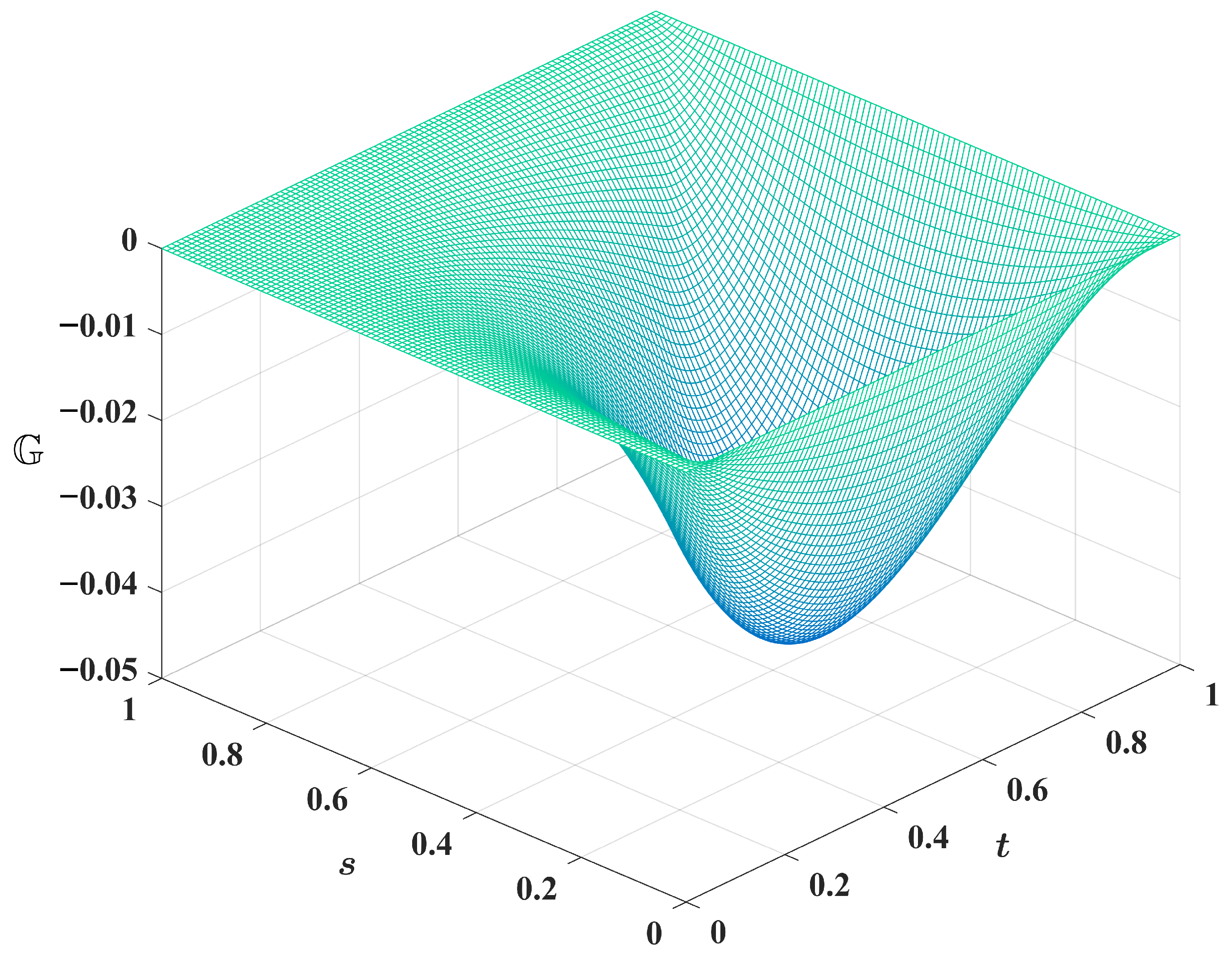
where Green’s function, denoted by $\mathbb{G}(t,s)$, is described as

$$\mathbb{G}(t,s)=\left\{\begin{array}{cc}-{\displaystyle \frac{{(t-\alpha )}^2{(\beta -s)}^2}{2{(\beta -\alpha )}^2}}+{\displaystyle \frac{{(t-s)}^2}{2}}\hfill & \mathrm{if}\alpha \le s\le t\le \beta ,\hfill \\ -{\displaystyle \frac{{(t-\alpha )}^2{(\beta -s)}^2}{2{(\beta -\alpha )}^2}}\hfill & \mathrm{if}\alpha \le t\le s\le \beta .\hfill \end{array}\right.$$

(20)

Figure 1 shows the plot of the function (20) that is involved in the integral issue (19) where $\alpha =0$ and $\beta =1$. The operator $\mathfrak{T}:C^2[\alpha ,\beta ]\to C^3[\alpha ,\beta ]$ is now introduced and defined by the statement

$$\mathfrak{T}u\left(t\right)={\int }_{\alpha }^{\beta }\mathbb{G}(t,s)q(s,u\left(s\right),u^{\prime }\left(s\right),u^{″}\left(s\right))ds.$$

(21)

Determining the fixed points of the operator $\mathfrak{T}$ is therefore the same as resolving the differential equation’s boundary value issue. Stated differently, the process of solving the BVP can be reformulated as locating a fixed point of an operator that is appropriately described.

Lemma 4. 

Equation (20) states that the Green function $\mathbb{G}(t,s)$ meets the following inequalities:

$${\int }_{\alpha }^{\beta }\mid \mathbb{G}(t,s)\mid ds\le {\displaystyle \frac{{(\beta -\alpha )}^3}{3}},{\int }_{\alpha }^{\beta }\mid {\mathbb{G}}_t(t,s)\mid ds\le {\displaystyle \frac{5{(\beta -\alpha )}^2}{6}},$$

and

$${\int }_{\alpha }^{\beta }\mid {\mathbb{G}}_{tt}(t,s)\mid ds\le {\displaystyle \frac{4(\beta -\alpha )}{3}}$$

for $t\in [\alpha ,\beta ]$.

Proof. 

The integral of $\mid \mathbb{G}(t,s)\mid$ should first be expressed as

$$\begin{array}{ccc}\hfill {\int }_{\alpha }^{\beta }\mid \mathbb{G}(t,s)\mid ds& =& {\int }_{\alpha }^t\left|-{\displaystyle \frac{{(t-\alpha )}^2{(\alpha -s)}^2}{2{(\beta -\alpha )}^2}}+{\displaystyle \frac{{(t-s)}^2}{2}}\right|ds+{\int }_t^{\beta }\left|-{\displaystyle \frac{{(t-\alpha )}^2{(\beta -s)}^2}{2{(\beta -\alpha )}^2}}\right|ds\hfill \\ & \le & {\int }_{\alpha }^t\left[{\displaystyle \frac{{(t-\alpha )}^2{(\beta -s)}^2}{2{(\beta -\alpha )}^2}}+{\displaystyle \frac{{(t-s)}^2}{2}}\right]ds+{\int }_t^{\beta }{\displaystyle \frac{{(t-\alpha )}^2{(\beta -s)}^2}{2{(\beta -\alpha )}^2}}ds\hfill \\ & =& -{\displaystyle \frac{{(t-\alpha )}^2{(\beta -t)}^3}{6{(\beta -\alpha )}^2}}+{\displaystyle \frac{{(t-\alpha )}^2{(\beta -\alpha )}^3}{6{(\beta -\alpha )}^2}}+{\displaystyle \frac{{(t-\alpha )}^3}{6}}+{\displaystyle \frac{{(t-\alpha )}^2{(\beta -t)}^3}{6{(\beta -\alpha )}^2}}\hfill \\ & =& {\displaystyle \frac{{(t-\alpha )}^2(\beta -\alpha )}{6}}+{\displaystyle \frac{{(t-\alpha )}^3}{6}}\hfill \\ & \le & {\displaystyle \frac{{(\beta -\alpha )}^2(\beta -\alpha )}{6}}+{\displaystyle \frac{{(\beta -\alpha )}^3}{6}}\hfill \\ & =& {\displaystyle \frac{{(\beta -\alpha )}^3}{3}}.\hfill \end{array}$$

Similarly, we obtain

$$\begin{array}{ccc}\hfill {\int }_{\alpha }^{\beta }\mid {\mathbb{G}}_t(t,s)\mid ds& =& {\int }_{\alpha }^t\left|-{\displaystyle \frac{(t-\alpha ){(\beta -s)}^2}{{(\beta -\alpha )}^2}}+(t-s)\right|ds+{\int }_t^{\beta }\left|-{\displaystyle \frac{(t-\alpha ){(\beta -s)}^2}{{(\beta -\alpha )}^2}}\right|ds\hfill \\ & \le & {\int }_{\alpha }^t\left[{\displaystyle \frac{(t-\alpha ){(\beta -s)}^2}{{(\beta -\alpha )}^2}}+(t-s)\right]ds+{\int }_t^{\beta }{\displaystyle \frac{(t-\alpha ){(\beta -s)}^2}{{(\beta -\alpha )}^2}}ds\hfill \\ & =& -{\displaystyle \frac{(t-\alpha ){(\beta -t)}^3}{3{(\beta -\alpha )}^2}}+{\displaystyle \frac{(t-\alpha ){(\beta -\alpha )}^3}{3{(\beta -\alpha )}^2}}+{\displaystyle \frac{{(t-\alpha )}^2}{2}}+{\displaystyle \frac{(t-\alpha ){(\beta -t)}^3}{3{(\beta -\alpha )}^2}}\hfill \\ & =& {\displaystyle \frac{(t-\alpha )(\beta -\alpha )}{3}}+{\displaystyle \frac{{(t-\alpha )}^2}{2}}\hfill \\ & \le & {\displaystyle \frac{{(\beta -\alpha )}^2}{3}}+{\displaystyle \frac{{(\beta -\alpha )}^2}{2}}\hfill \\ & =& {\displaystyle \frac{5{(\beta -\alpha )}^2}{6}}.\hfill \end{array}$$

Finally, the integral of $\mid {\mathbb{G}}_{tt}(t,s)\mid$ yields

$$\begin{array}{ccc}\hfill {\int }_{\alpha }^{\beta }\mid {\mathbb{G}}_{tt}(t,s)\mid ds& =& {\int }_{\alpha }^t\left|-{\displaystyle \frac{{(\beta -s)}^2}{{(\beta -\alpha )}^2}}+1\right|ds+{\int }_t^{\beta }\left|-{\displaystyle \frac{{(\beta -s)}^2}{{(\beta -\alpha )}^2}}\right|ds\hfill \\ & \le & {\int }_{\alpha }^t\left[{\displaystyle \frac{{(\beta -s)}^2}{{(\beta -\alpha )}^2}}+1\right]ds+{\int }_t^{\beta }{\displaystyle \frac{{(\beta -s)}^2}{{(\beta -\alpha )}^2}}ds\hfill \\ & =& -{\displaystyle \frac{{(\beta -t)}^3}{3{(\beta -\alpha )}^2}}+{\displaystyle \frac{{(\beta -\alpha )}^3}{3{(\beta -\alpha )}^2}}+(t-\alpha )+{\displaystyle \frac{{(\beta -t)}^3}{3{(\beta -\alpha )}^2}}\hfill \\ & =& {\displaystyle \frac{(\beta -\alpha )}{3}}+(t-\alpha )\hfill \\ & \le & {\displaystyle \frac{(\beta -\alpha )}{3}}+(\beta -\alpha )\hfill \\ & =& {\displaystyle \frac{4(\beta -\alpha )}{3}}.\hfill \end{array}$$

This completes the proof. □

Theorem 2. 

Let $\gamma \in \mathrm{\Gamma }$ and suppose there exists a function $u_0\left(t\right)\in C^2[\alpha ,\beta ]$ such that $\gamma (u_0\left(t\right),\mathfrak{T}{u}_0\left(t\right))\ge 0\mathit{for}\mathit{all}t\in [\alpha ,\beta ]$. The derivatives of the continuous function q with respect to u, $u^{\prime }$, and $u^{″}$ are assumed to have boundaries of ${\mathfrak{L}}_1$, ${\mathfrak{L}}_2$, and ${\mathfrak{L}}_3$, respectively. Let

$$\mathfrak{L}:=max\{{\mathfrak{L}}_1,{\mathfrak{L}}_2,{\mathfrak{L}}_3\}$$

and

$$\mathfrak{L}\le {\displaystyle \frac{1}{\xi }}\left({\displaystyle \frac{ln(1+\parallel u-v\parallel +|\parallel u-\mathfrak{T}u\parallel -\parallel v-\mathfrak{T}v\parallel \left|\right)}{\parallel u-v\parallel +|\parallel u-\mathfrak{T}u\parallel -\parallel v-\mathfrak{T}v\parallel |}}\right),$$

where $\xi ={\displaystyle \frac{{(b-a)}^3}{3}}+{\displaystyle \frac{5{(b-a)}^2}{6}}+{\displaystyle \frac{4(b-a)}{3}}$. According to these assumptions, $\mathfrak{T}$ has a fixed point in $C^2[\alpha ,\beta ]$ that a solution to the integral problem (21).

Proof. 

Under these presumptions, $D\left(\mathfrak{T}\right)=\{u\in C^2[\alpha ,\beta ]:(u,\mathfrak{T}u)\in E\left(G_{\gamma }\right)\}\ne ⌀$ and the $G_D$-continuity, we have left to show that $\mathfrak{T}$ is a G-connected contraction. Suppose that ${\displaystyle \parallel u\parallel =\underset{t\in [\alpha ,\beta ]}{max}\left[\right|u\left(t\right)|+|u^{\prime }\left(t\right)|+|u^{″}\left(t\right)\left|\right]}$ is $C^2[\alpha ,\beta ]$’s norm. The definition of $\mathfrak{T}$ can be found in Equation (21). First, observe that since $\mathbb{G}$’s differentiability permits differentiation under the integral sign, $\mathfrak{T}$ does, in fact, map into $C^3[\alpha ,\beta ]$. Therefore,

$${\left(\mathfrak{T}u\right)}^{\prime }\left(t\right)={\int }_{\alpha }^{\beta }{\mathbb{G}}_t(t,s)q(s,u\left(s\right),u^{\prime }\left(s\right),u^{″}\left(s\right))ds,$$

and

$${\left(\mathfrak{T}u\right)}^{″}\left(t\right)={\int }_{\alpha }^{\beta }{\mathbb{G}}_{tt}(t,s)q(s,u\left(s\right),u^{\prime }\left(s\right),u^{″}\left(s\right))ds.$$

The calculation in Lemma 4 yields

$${\int }_{\alpha }^{\beta }\mid \mathbb{G}(t,s)\mid ds\le {\displaystyle \frac{{(\beta -\alpha )}^3}{3}}.$$

Given that $q_u$, $q_{u^{\prime }}$, and $q_{u^{″}}$ are constrained by ${\mathfrak{L}}_1$, ${\mathfrak{L}}_2$, and ${\mathfrak{L}}_3$, respectively, and the mean value theorem is used, we derive

$$\begin{array}{ccc}& & \left|\right(\mathfrak{T}u\left)\right(t)-(\mathfrak{T}v\left)\right(t\left)\right|\hfill \\ & =& \left|{\int }_{\alpha }^{\beta }\mathbb{G}(t,s)[q(s,u\left(s\right),u^{\prime }\left(s\right),u^{″}\left(s\right))-q(s,v\left(s\right),v^{\prime }\left(s\right),v^{″}\left(s\right))]ds\right|\hfill \\ & \le & {\int }_{\alpha }^{\beta }\left|\mathbb{G}(t,s)\right|\left|q(s,u\left(s\right),u^{\prime }\left(s\right),u^{″}\left(s\right))-q(s,v\left(s\right),v^{\prime }\left(s\right),v^{″}\left(s\right))\right|ds\hfill \\ & \le & {\int }_{\alpha }^{\beta }\left|\mathbb{G}(t,s)\right|\left|q_u(u\left(s\right)-v\left(s\right))+q_{u^{\prime }}(u^{\prime }\left(s\right)-v^{\prime }\left(s\right))+q_{u^{″}}(u^{″}\left(s\right)-v^{″}\left(s\right))\right|ds\hfill \\ & \le & \underset{s\in [\alpha ,\beta ]}{max}\left[\right|q_u\left|\right|u\left(s\right)-v\left(s\right)|+|q_{u^{\prime }}\left|\right|u^{\prime }\left(s\right)-v^{\prime }\left(s\right)|+|q_{u^{″}}\left|\right|u^{″}\left(s\right)-v^{″}\left(s\right)\left|\right]{\int }_{\alpha }^{\beta }\left|\mathbb{G}(t,s)\right|ds\hfill \\ & \le & \underset{s\in [\alpha ,\beta ]}{max}[{\mathfrak{L}}_1|u\left(s\right)-v\left(s\right)|+{\mathfrak{L}}_2|u^{\prime }\left(s\right)-v^{\prime }\left(s\right)|+{\mathfrak{L}}_3|u^{″}\left(s\right)-v^{″}\left(s\right)\left|\right]{\int }_{\alpha }^{\beta }\left|\mathbb{G}(t,s)\right|ds\hfill \\ & \le & \mathfrak{L}\underset{s\in [\alpha ,\beta ]}{max}\left[\right|u\left(s\right)-v\left(s\right)|+|u^{\prime }\left(s\right)-v^{\prime }\left(s\right)|+|u^{″}\left(s\right)-v^{″}\left(s\right)\left|\right]{\int }_{\alpha }^{\beta }\left|\mathbb{G}(t,s)\right|ds\hfill \\ & =& \mathfrak{L}\parallel u-v\parallel {\int }_{\alpha }^{\beta }\left|\mathbb{G}(t,s)\right|ds\hfill \\ & \le & {\displaystyle \frac{{(\beta -\alpha )}^3}{3}}\mathfrak{L}\parallel u-v\parallel .\hfill \end{array}$$

(22)

Furthermore,

$${\int }_{\alpha }^{\beta }\mid {\mathbb{G}}_t(t,s)\mid ds\le {\displaystyle \frac{5{(\beta -\alpha )}^2}{6}}$$

(23)

and

$${\int }_{\alpha }^{\beta }\mid {\mathbb{G}}_{tt}(t,s)\mid ds\le {\displaystyle \frac{4(\beta -\alpha )}{3}}.$$

(24)

are provided by the results in Lemma 4. Likewise, by employing inequalities (23) and (24) and the examination of the quantity (22), we arrive at

$$\begin{array}{ccc}\hfill {|\left(\mathfrak{T}u\right)}^{\prime }\left(t\right)-{\left(\mathfrak{T}v\right)}^{\prime }\left(t\right)|& \le & \mathfrak{L}\parallel u-v\parallel {\int }_{\alpha }^{\beta }\mid {\mathbb{G}}_t(t,s)\mid ds\hfill \\ \hfill & \le & {\displaystyle \frac{5{(\beta -\alpha )}^2}{6}}\mathfrak{L}\parallel u-v\parallel \hfill \end{array}$$

(25)

and

$$\begin{array}{ccc}\hfill {|\left(\mathfrak{T}u\right)}^{″}\left(t\right)-{\left(\mathfrak{T}v\right)}^{″}\left(t\right)|& \le & \mathfrak{L}\parallel u-v\parallel {\int }_{\alpha }^{\beta }\mid {\mathbb{G}}_{tt}(t,s)\mid ds\hfill \\ \hfill & \le & {\displaystyle \frac{4(\beta -\alpha )}{3}}\mathfrak{L}\parallel u-v\parallel .\hfill \end{array}$$

(26)

When the hypothesis of the theorem is combined with the left-hand side of inequalities that came before it, (22), (25) and (26), we obtain

$$\begin{array}{ccc}\hfill \parallel \mathfrak{T}u-\mathfrak{T}v\parallel & \le & \left({\displaystyle \frac{{(\beta -\alpha )}^3}{3}}+{\displaystyle \frac{5{(\beta -\alpha )}^2}{6}}+{\displaystyle \frac{4(\beta -\alpha )}{3}}\right)\mathfrak{L}\parallel u-v\parallel \hfill \\ & \le & \left({\displaystyle \frac{ln(1+\mathfrak{M})}{\mathfrak{M}}}\right)\mathfrak{M}\hfill \end{array}$$

where

$$\mathfrak{M}=\parallel u-v\parallel +|\parallel u-\mathfrak{T}u\parallel -\parallel v-\mathfrak{T}v\parallel |.$$

Therefore, $\mathfrak{T}$ is a G-connected contraction from the complete space, $C^2[a,b]$, to $C^3[a,b]\subset C^2[a,b]$. As a result, the desired solution, u, is its fixed point. □

The problem (17) with the conditions (18), which are meant to be solved numerically, is now approached iteratively. The fundamental concept of the suggested plan is to use the well-known Picard fixed-point iterative technique. For this, an integral operator that is stated in terms of the Green’s function corresponding to the linear portion of the problem (17) is meticulously defined. Start by defining the integral operator

$$\mathfrak{P}u={\int }_{\alpha }^{\beta }\mathbb{G}(t,s)u^{‴}\left(s\right)ds.$$

(27)

When $q(s,u\left(s\right),u^{\prime }\left(s\right),u^{″}\left(s\right))$ is added and subtracted from within the integrand using the relation (19), the outcome is

$$\begin{array}{cc}\hfill \mathfrak{P}u& ={\int }_{\alpha }^{\beta }\mathbb{G}(t,s)\left(u^{‴}\left(s\right)-q(s,u\left(s\right),u^{\prime }\left(s\right),u^{″}\left(s\right))+q(s,u\left(s\right),u^{\prime }\left(s\right),u^{″}\left(s\right))\right)ds\hfill \\ \hfill & ={\int }_{\alpha }^{\beta }\mathbb{G}(t,s)\left(u^{‴}\left(s\right)-q(s,u\left(s\right),u^{\prime }\left(s\right),u^{″}\left(s\right))\right)ds\hfill \\ \hfill & +{\int }_{\alpha }^{\beta }\mathbb{G}(t,s)\left(q(s,u\left(s\right),u^{\prime }\left(s\right),u^{″}\left(s\right))\right)ds\hfill \\ \hfill & ={\int }_{\alpha }^{\beta }\mathbb{G}(t,s)\left(u^{‴}\left(s\right)-q(s,u\left(s\right),u^{\prime }\left(s\right),u^{″}\left(s\right))\right)ds+u.\hfill \end{array}$$

(28)

The operator $\mathfrak{P}$ yields

$$u_{n+1}=\mathfrak{P}{u}_n=u_n+{\int }_{\alpha }^{\beta }\mathbb{G}(t,s)(u_n^{‴}\left(s\right)-q(s,u_n\left(s\right),u_n^{\prime }\left(s\right),u_n^{″}\left(s\right)))ds,$$

(29)

when Green–Picard’s fixed-point iteration approximation is applied. Take into consideration the following unique situation:

$$u^{‴}\left(t\right)=q(t,u\left(t\right),u^{\prime }\left(t\right),u^{″}\left(t\right)),\mathrm{for}\mathrm{all}t\in [0,1],$$

(30)

in accordance with the circumstances

$$u\left(0\right)=u^{\prime }\left(0\right)=0\mathrm{and}u\left(1\right)=0.$$

(31)

Subject to the Green’s function, the iterative scheme is expressed as

$$u_{n+1}=\mathfrak{P}{u}_n=u_n+{\int }_0^1{\mathbb{G}}^{*}(t,s)(u_n^{‴}\left(s\right)-q(s,u_n\left(s\right),u_n^{\prime }\left(s\right),u_n^{″}\left(s\right)))ds,$$

(32)

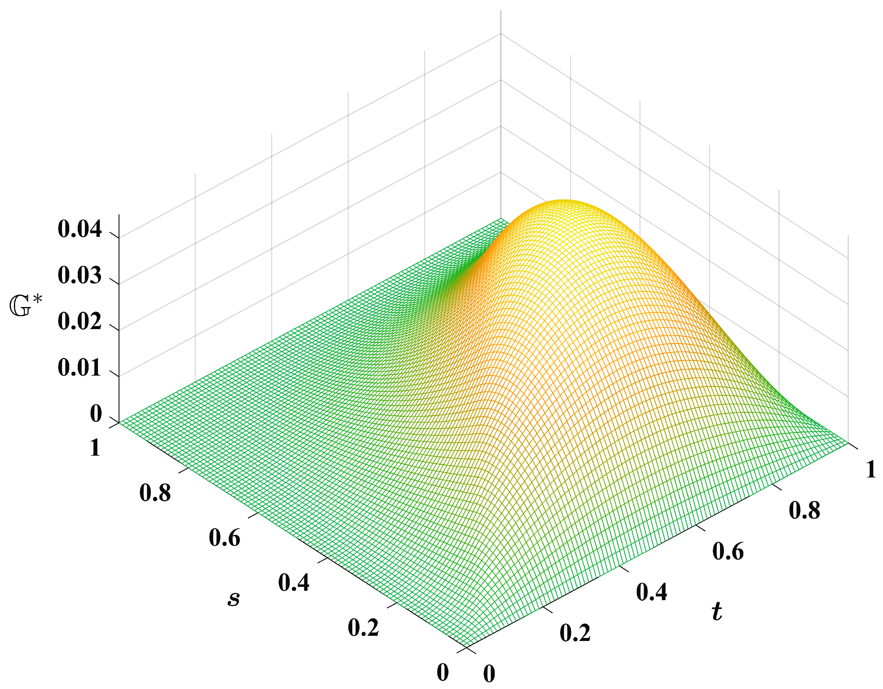
where

$${\mathbb{G}}^{*}(t,s)=\left\{\begin{array}{cc}{\displaystyle \frac{t^2{(1-s)}^2}{2}}-{\displaystyle \frac{{(t-s)}^2}{2}}\hfill & \mathrm{if}0\le s\le t\le 1,\hfill \\ {\displaystyle \frac{t^2{(1-s)}^2}{2}}\hfill & \mathrm{if}0\le t\le s\le 1.\hfill \end{array}\right.$$

(33)

The plot of the function (33) involved in the iterative scheme (32) is given in Figure 2.

To demonstrate the theorem, we will work within the function space $C^2[0,1]$, which allows us to handle the second-order derivatives that appear in the differential equation. To measure the magnitude of functions within this space, we establish the norm

$${\displaystyle \parallel u\parallel =\underset{t\in [0,1]}{max}\left[\right|u\left(t\right)|+|u^{\prime }\left(t\right)|+|u^{″}\left(t\right)\left|\right].}$$

Theorem 3. 

Let $\gamma \in \mathrm{\Gamma }$ and suppose there exists a function $u_0\left(t\right)\in C^2[0,1]$ such that

$\gamma (u_0\left(t\right),\mathfrak{P}{u}_0\left(t\right))\ge 0\mathit{for}\mathit{all}t\in [0,1]$. The derivatives of the continuous function q with respect to u, $u^{\prime }$, and $u^{″}$ are assumed to have boundaries of ${\mathfrak{L}}_1$, ${\mathfrak{L}}_2$, and ${\mathfrak{L}}_3$, respectively. Let

$$\mathfrak{L}:=max\{{\mathfrak{L}}_1,{\mathfrak{L}}_2,{\mathfrak{L}}_3\}$$

and

$$\mathfrak{L}\le {\displaystyle \frac{2}{5}}\left({\displaystyle \frac{ln(1+\parallel u_n-v_n\parallel +|\parallel u_n-\mathfrak{P}{u}_n\parallel -\parallel v_n-\mathfrak{P}{v}_n\parallel \left|\right)}{\parallel u_n-v_n\parallel +|\parallel u_n-\mathfrak{P}{u}_n\parallel -\parallel v_n-\mathfrak{P}{v}_n\parallel |}}\right).$$

According to these assumptions, $\mathfrak{P}$ has a fixed point in $C^2[0,1]$ that is a solution to the iterative (32).

Proof. 

$$\begin{array}{ccc}\hfill \mathfrak{P}{u}_n& =& u_n+{\mathbb{G}}^{*}(t,1)u_n^{″}\left(1\right)-{\mathbb{G}}^{*}(t,0)u_n^{″}\left(0\right)-{\mathbb{G}}_s^{*}(t,1)u_n^{\prime }\left(1\right)+{\mathbb{G}}_s^{*}(t,0)u_n^{\prime }\left(0\right)\hfill \\ & & +{\mathbb{G}}_{ss}^{*}(t,1)u_n\left(1\right)+(t^2-1)u_n\left(t\right)-t^2{u}_n\left(t\right)-{\mathbb{G}}_{ss}^{*}(t,0)u_n\left(0\right)\hfill \\ \hfill & & -{\int }_0^1{\mathbb{G}}^{*}(t,s)q(s,u_n\left(s\right),u_n^{\prime }\left(s\right),u_n^{″}\left(s\right))ds,\hfill \end{array}$$

(34)

is obtained by simplifying the iterative process (32) and carrying out three integrations by parts on the integrand’s initial term, where ${\mathbb{G}}^{*}(t,s)$ is the function provided in Equation (33). The equivalent homogeneous requirements, ${\mathbb{G}}^{*}(t,0)={\mathbb{G}}^{*}(t,1)=0$, are easily shown to be satisfied by ${\mathbb{G}}^{*}(t,s)$. The scheme (35) reduces to

$$\mathfrak{P}{u}_n=-{\mathbb{G}}_s^{*}(t,1)u_n^{\prime }\left(1\right)-{\int }_0^1{\mathbb{G}}^{*}(t,s)q(s,u_n\left(s\right),u_n^{\prime }\left(s\right),u_n^{″}\left(s\right))ds$$

since $u_n$ satisfies the boundaries $u_n\left(0\right)=u_n^{\prime }\left(0\right)=0$ and $u_n\left(1\right)=0$. The value of the function ${\mathbb{G}}^{*}$ presented in Equation (33) indicates that ${\mathbb{G}}_s^{*}(t,1)=0$, which is evident from the previous computations. Given that $q_{u_n}$, $q_{u_n^{\prime }}$, and $q_{u_n^{″}}$ are bounded by ${\mathfrak{L}}_1$, ${\mathfrak{L}}_2$, and ${\mathfrak{L}}_3$, respectively, and the mean value theorem is applied, we come to

$$\begin{array}{ccc}& & |\left(\mathfrak{P}{u}_n\right)\left(t\right)-\left(\mathfrak{P}{v}_n\right)\left(t\right)|\hfill \\ & =& \left|{\int }_0^1{\mathbb{G}}^{*}(t,s)[q(s,u_n\left(s\right),u_n^{\prime }\left(s\right),u_n^{″}\left(s\right))-q(s,v_n\left(s\right),v_n^{\prime }\left(s\right),v_n^{″}\left(s\right))]ds\right|\hfill \\ & \le & {\int }_0^1\left|{\mathbb{G}}^{*}(t,s)\right|\left|q(s,u_n\left(s\right),u_n^{\prime }\left(s\right),u_n^{″}\left(s\right))-q(s,v_n\left(s\right),v_n^{\prime }\left(s\right),v_n^{″}\left(s\right))\right|ds\hfill \\ & \le & {\int }_0^1\left|{\mathbb{G}}^{*}(t,s)\right|\left|q_{u_n}(u_n\left(s\right)-v_n\left(s\right))+q_{u_n^{\prime }}(u_n^{\prime }\left(s\right)-v_n^{\prime }\left(s\right))+q_{u_n^{″}}(u_n^{″}\left(s\right)-v_n^{″}\left(s\right))\right|ds\hfill \\ & \le & \underset{s\in [0,1]}{max}\left[\right|q_{u_n}\left|\right|u_n\left(s\right)-v_n\left(s\right)|+|q_{u_n^{\prime }}\left|\right|u_n^{\prime }\left(s\right)-v_n^{\prime }\left(s\right)|+|q_{u_n^{″}}\left|\right|u_n^{″}\left(s\right)-v_n^{″}\left(s\right)\left|\right]{\int }_0^1\left|{\mathbb{G}}^{*}(t,s)\right|ds\hfill \\ & \le & \underset{s\in [0,1]}{max}[{\mathfrak{L}}_1|u_n\left(s\right)-v_n\left(s\right)|+{\mathfrak{L}}_2|u_n^{\prime }\left(s\right)-v_n^{\prime }\left(s\right)|+{\mathfrak{L}}_3|u_n^{″}\left(s\right)-v_n^{″}\left(s\right)\left|\right]{\int }_0^1\left|{\mathbb{G}}^{*}(t,s)\right|ds\hfill \\ & \le & \mathfrak{L}\underset{s\in [0,1]}{max}\left[\right|u_n\left(s\right)-v_n\left(s\right)|+|u_n^{\prime }\left(s\right)-v_n^{\prime }\left(s\right)|+|u_n^{″}\left(s\right)-v_n^{″}\left(s\right)\left|\right]{\int }_0^1\left|{\mathbb{G}}^{*}(t,s)\right|ds\hfill \\ & =& \mathfrak{L}\parallel u_n-v_n\parallel {\int }_0^1\left|{\mathbb{G}}^{*}(t,s)\right|ds\hfill \\ & \le & {\displaystyle \frac{1}{3}}\mathfrak{L}\parallel u_n-v_n\parallel .\hfill \end{array}$$

(35)

Additionally, the assessments that follow are simple to complete:

$${\int }_0^1\mid {\mathbb{G}}_t^{*}(t,s)\mid ds\le {\displaystyle \frac{5}{6}}$$

(36)

and

$${\int }_0^1\mid {\mathbb{G}}_{tt}^{*}(t,s)\mid ds\le {\displaystyle \frac{4}{3}}.$$

(37)

Similarly, by employing inequalities (36) and (37) and the analysis, the quantity (35) yields

$$\begin{array}{ccc}\hfill |{\left(\mathfrak{P}{u}_n\right)}^{\prime }\left(t\right)-{\left(\mathfrak{P}{v}_n\right)}^{\prime }\left(t\right)|& \le & \mathfrak{L}\parallel u_n-v_n\parallel {\int }_0^1\mid {\mathbb{G}}_t^{*}(t,s)\mid ds\hfill \\ \hfill & \le & {\displaystyle \frac{5}{6}}\mathfrak{L}\parallel u_n-v_n\parallel \hfill \end{array}$$

(38)

and

$$\begin{array}{ccc}\hfill |{\left(\mathfrak{P}{u}_n\right)}^{″}\left(t\right)-{\left(\mathfrak{P}{v}_n\right)}^{″}\left(t\right)|& \le & \mathfrak{L}\parallel u_n-v_n\parallel {\int }_0^1\mid {\mathbb{G}}_{tt}^{*}(t,s)\mid ds\hfill \\ \hfill & \le & {\displaystyle \frac{4}{3}}\mathfrak{L}\parallel u_n-v_n\parallel .\hfill \end{array}$$

(39)

After arranging, we obtain

$$\begin{array}{ccc}\hfill \parallel \mathfrak{P}{u}_n-\mathfrak{P}{v}_n\parallel & \le & \left({\displaystyle \frac{1}{3}}+{\displaystyle \frac{5}{6}}+{\displaystyle \frac{4}{3}}\right)\mathfrak{L}\parallel u_n-v_n\parallel \hfill \end{array}$$

(40)

$$\begin{array}{ccc}& =& {\displaystyle \frac{5}{2}}\mathfrak{L}\parallel u_n-v_n\parallel \hfill \end{array}$$

(41)

$$\begin{array}{ccc}& \le & \left({\displaystyle \frac{ln(1+{\mathfrak{M}}_n)}{{\mathfrak{M}}_n}}\right){\mathfrak{M}}_n\hfill \end{array}$$

(42)

by adding the hypothesis of the theorem to the left-hand side of the preceding inequalities that came before it, (35), (38) and (39), where

$${\mathfrak{M}}_n=\parallel u_n-v_n\parallel +|\parallel u_n-\mathfrak{P}{u}_n\parallel -\parallel v_n-\mathfrak{P}{v}_n\parallel |.$$

Therefore, $\mathfrak{P}$ is a G-connected contraction from $C^2[a,b]$ to $C^3[a,b]\subset C^2[a,b]$. Therefore, it has the desired outcome. □

6. Numerical Examples

Two numerical examples of boundary value issues involving third-order nonlinear differential equations are given in this section. Example 5 considers equations of the form given in Equation (30) with homogeneous boundary conditions specified in Equation (31), while Example 6 examines equations of the form presented in Equation (30) with non-homogeneous boundary conditions. These examples show the efficacy of the suggested iterative strategy and validate the theoretical findings produced. Both instances have known exact solutions. The following metrics are used to assess the accuracy of the present iterative approach:

(1)

Absolute Error (AE):

The definition of the absolute error at any given point t is

$$\begin{array}{c}\hfill \mathrm{AE}\left(n\right)=\left|u_n\left(t\right)-u\left(t\right)\right|,\end{array}$$

where the exact solution is $u\left(t\right)$ and the approximate solution $u_n\left(t\right)$ is derived using the suggested approach. This measure expresses how much the approximate and exact answers differ from one another.

(2)

Mean Absolute Error (MAE):

The mean absolute error over N evaluation points is given by

$$\begin{array}{c}\hfill \mathrm{MAE}={\displaystyle \frac{1}{N}}\sum _{i=1}^N\left|u_n\left(t\right)-u\left(t\right)\right|.\end{array}$$

Numerical simulations are conducted in this study using MATLAB software (Version 2018a).

Example 5. 

Consider the third-order nonlinear differential equation

$$u^{‴}\left(t\right)+3u\left(t\right)u^{″}\left(t\right)-2{\left(u^{\prime }\left(t\right)\right)}^2=6-2t^2,$$

(43)

with the conditions of the boundaries

$$u\left(0\right)=u^{\prime }\left(0\right)=u\left(1\right)=0.$$

(44)

The precise answer to this problem is

$$u\left(t\right)=t^3-t^2.$$

(45)

The following is the definition of the function q:

$$\begin{array}{c}\hfill q(t,u,u^{\prime },u^{″})=-3u\left(t\right)u^{″}\left(t\right)+2{\left(u^{\prime }\left(t\right)\right)}^2+6-2t^2.\end{array}$$

From Equations (32) and (33), the iterative scheme for solving this example is formulated as

$$\begin{array}{cc}\hfill u_{n+1}\left(t\right)& =u_n\left(t\right)\hfill \\ \hfill & +\underset{0}{\overset{t}{\int }}\left[{\displaystyle \frac{t^2{(1-s)}^2}{2}}-{\displaystyle \frac{{(t-s)}^2}{2}}\right]\left[u_n^{‴}\left(s\right)-\left(-3u_n\left(s\right)u_n^{″}\left(s\right)+2{\left(u_n^{\prime }\left(s\right)\right)}^2+6-2s^2\right)\right]ds\hfill \\ \hfill & +\underset{t}{\overset{1}{\int }}\left[{\displaystyle \frac{t{(1-s)}^2}{2}}\right]\left[u_n^{‴}\left(s\right)-\left(-3u_n\left(s\right)u_n^{″}\left(s\right)+2{\left(u_n^{\prime }\left(s\right)\right)}^2+6-2s^2\right)\right]ds.\hfill \end{array}$$

(46)

The initial approximation $u_0\left(t\right)=0$, which satisfies the homogeneous problem $u^{‴}\left(t\right)=0$ and the boundary requirements given in Equation (44), is where we begin implementing the presented iterative technique.

Table 1. Maximum and mean absolute errors for iterations 1 through 5.

Number of Iterations	1	2	3	4	5
Maximum Absolute Error	$1.0731\times {10}^{-2}$	$1.2640\times {10}^{-3}$	$1.4311\times {10}^{-4}$	$1.5687\times {10}^{-5}$	$1.7055\times {10}^{-6}$
MAE	$6.0806\times {10}^{-3}$	$7.0255\times {10}^{-4}$	$7.8489\times {10}^{-5}$	$8.5838\times {10}^{-6}$	$9.3323\times {10}^{-7}$

presents the maximum and mean absolute errors obtained using the iterative scheme described in Equation (46) for iterations 1 through 5 of this BVP. The results demonstrate that both error measures converge to zero as the number of iterations increases. Additionally,

Table 2. Comparison of the exact and approximate solutions at iterations 1 through 5.

t	Exact Solution	Approximate Solution
		$\mathit{n}=\mathbf{1}$	$\mathit{n}=\mathbf{2}$	$\mathit{n}=\mathbf{3}$	$\mathit{n}=\mathbf{4}$	$\mathit{n}=\mathbf{5}$
0	0	0	0	0	0	0
$0.1$	$-0.0090$	$-0.0087$	$-0.0090$	$-0.0090$	$-0.0090$	$-0.0090$
$0.2$	$-0.0320$	$-0.0307$	$-0.0319$	$-0.0320$	$-0.0320$	$-0.0320$
$0.3$	$-0.0630$	$-0.0601$	$-0.0627$	$-0.0630$	$-0.0630$	$-0.0630$
$0.4$	$-0.0960$	$-0.0910$	$-0.0955$	$-0.0959$	$-0.0960$	$-0.0960$
$0.5$	$-0.1250$	$-0.1177$	$-0.1242$	$-0.1249$	$-0.1250$	$-0.1250$
$0.6$	$-0.1440$	$-0.1346$	$-0.1429$	$-0.1439$	$-0.1440$	$-0.1440$
$0.7$	$-0.1470$	$-0.1363$	$-0.1457$	$-0.1469$	$-0.1470$	$-0.1470$
$0.8$	$-0.1280$	$-0.1176$	$-0.1267$	$-0.1279$	$-0.1280$	$-0.1280$
$0.9$	$-0.0810$	$-0.0737$	$-0.0801$	$-0.0809$	$-0.0810$	$-0.0810$
$1.0$	0	0	0	0	0	0

compares the exact and approximate solutions obtained at iterations 1 through 5 for any point x in the interval $[0,1]$, with a step size of 0.1.

Figure 3 shows the comparison of absolute errors at iterations 1 through 5. Additionally, Figure 4 provides a graphical representation of both the exact and approximate solutions at iteration 5. It indicates that approximate solutions are closer to the exact solutions for every point as the number of iterations increases.

Example 6. 

Consider the third-order nonlinear differential equation

$$u^{‴}\left(t\right)-e^{-t}{\left(u^{\prime }\left(t\right)\right)}^2=0,$$

(47)

with the non-homogeneous boundary conditions

$$u\left(0\right)=1,u^{\prime }\left(0\right)=1,\mathit{and}u\left(1\right)=e.$$

(48)

The precise answer to this problem is

$$u\left(t\right)=e^t.$$

(49)

The definition of the function q is as follows:

$$\begin{array}{c}\hfill q(t,u,u^{\prime },u^{″})=e^{-t}{\left(u^{\prime }\left(t\right)\right)}^2.\end{array}$$

The following is the expression for the fixed-point iterative strategy used to estimate the solution of this example:

$$\begin{array}{cc}\hfill u_{n+1}\left(t\right)& =u_n\left(t\right)+\underset{0}{\overset{t}{\int }}\left[{\displaystyle \frac{t^2{(1-s)}^2}{2}}-{\displaystyle \frac{{(t-s)}^2}{2}}\right]\left[u_n^{‴}\left(s\right)-e^{-s}{\left(u_n^{\prime }\left(s\right)\right)}^2\right]ds\hfill \\ \hfill & +\underset{t}{\overset{1}{\int }}\left[{\displaystyle \frac{t^2{(1-s)}^2}{2}}\right]\left[u_n^{‴}\left(s\right)-e^{-s}{\left(u_n^{\prime }\left(s\right)\right)}^2\right]ds,\hfill \end{array}$$

(50)

where the initial iterate $u_0\left(t\right)$ fulfilled the corresponding homogeneous problem $u^{‴}\left(t\right)=0$ and the non-homogeneous boundary requirements (48). Next, we apply the initial approximation, denoted as $u_0\left(t\right)=(e-2)t^2+t+1$; it is simple to observe that the specified initial function $u_0\left(t\right)$ satisfies the criteria of the homogeneous equation.

Table 3. Maximum and mean absolute errors for iterations 1 through 3.

Number of Iterations	1	2	3
Maximum Absolute Error	$2.7319\times {10}^{-3}$	$1.7958\times {10}^{-4}$	$5.5831\times {10}^{-5}$
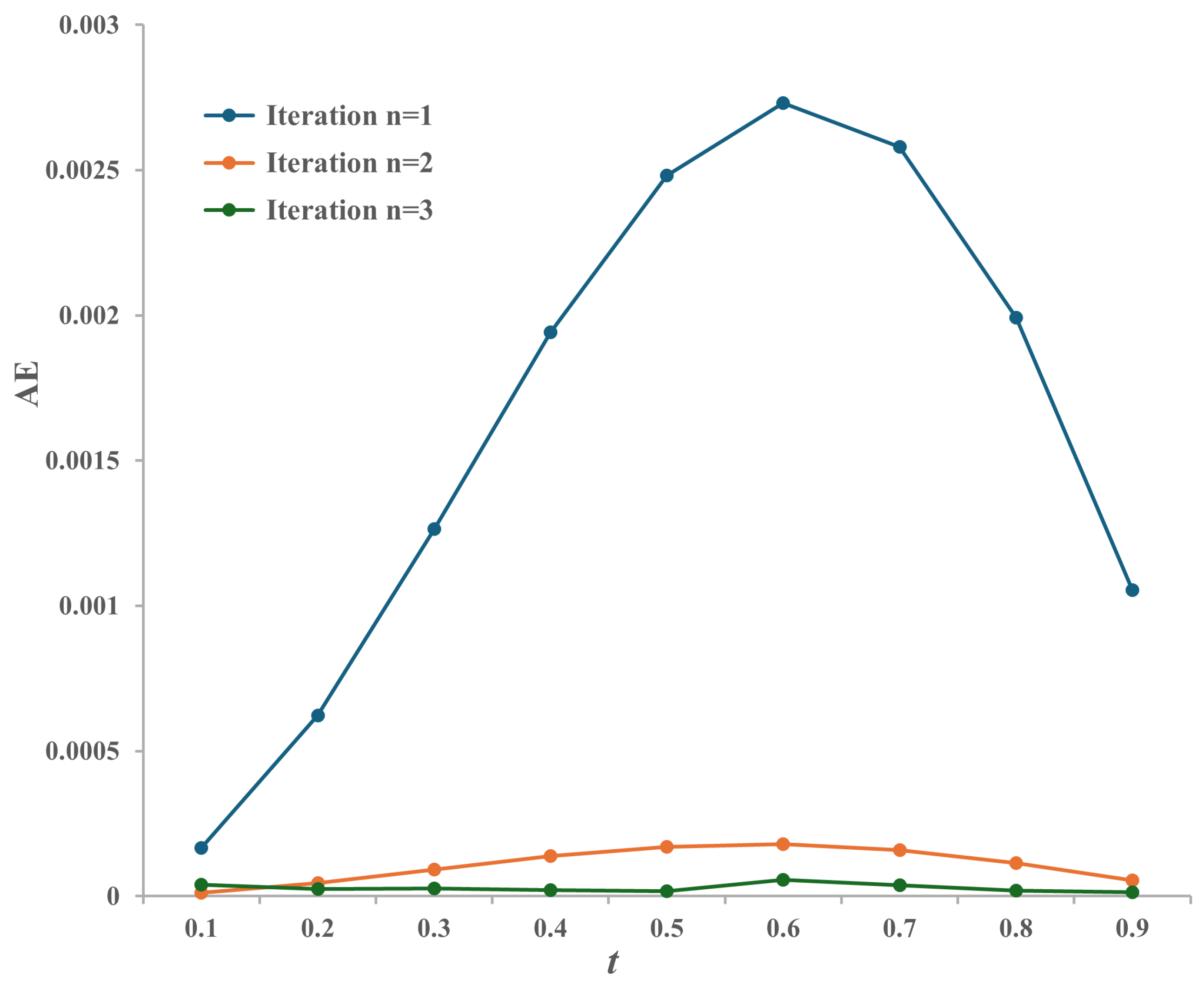
MAE	$1.6482\times {10}^{-3}$	$1.0753\times {10}^{-4}$	$2.8705\times {10}^{-5}$

summarizes the maximum and mean absolute errors computed using the proposed iterative scheme over three iterations for this BVP. The results indicate a consistent decrease in error measures as the number of iterations increases. The exact and approximate answers from iterations 1 through 3 are compared in detail in

Table 4. Comparison of the exact and approximate solutions at iterations 1 through 3.

t	Exact Solution	Approximate Solution
		$\mathit{n}=\mathbf{1}$	$\mathit{n}=\mathbf{2}$	$\mathit{n}=\mathbf{3}$
0	1.0000	1.0000	1.0000	1.0000
0.1	1.1052	1.1050	1.1052	1.1051
0.2	1.2214	1.2208	1.2214	1.2214
0.3	1.3499	1.3486	1.3500	1.3498
0.4	1.4918	1.4899	1.4920	1.4918
0.5	1.6487	1.6462	1.6489	1.6487
0.6	1.8221	1.8194	1.8223	1.8221
0.7	2.0138	2.0112	2.0139	2.0137
0.8	2.2255	2.2235	2.2257	2.2255
0.9	2.4596	2.4585	2.4597	2.4596
1	2.7183	2.7183	2.7183	2.7183

. With a 0.1 step size, it concentrates on locations inside the range [0, 1].

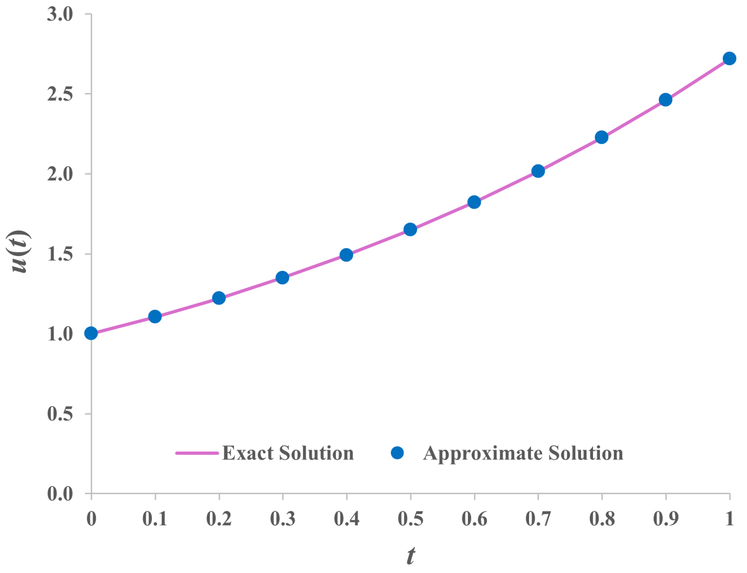
Figure 5 illustrates the absolute errors from iterations 1 to 3. Furthermore, Figure 6 presents the comparison of the exact solution alongside the approximate solution at the iteration 3. The results show that as the iterations progress, the approximate solutions increasingly align with the exact solutions at each point.

The numerical results presented in Table 1, Table 2, Table 3 and Table 4 and illustrated in Figure 3, Figure 4, Figure 5 and Figure 6 provide strong support for the accuracy and convergence of the proposed method. Notably, both the maximum and mean absolute errors consistently decreased with each iteration, demonstrating the method’s reliable convergence behavior. A detailed comparison between the exact and approximate solutions across different iteration levels further confirms the method’s precision. This is particularly clear in Figure 4 and Figure 6, where the approximate solutions closely align with the exact ones by the third and fifth iterations, respectively. These findings suggest that the proposed approach offers a reliable and efficient tool for analyzing and computing solutions to third-order nonlinear differential equations, under both homogeneous and nonhomogeneous boundary conditions. Its strong convergence properties and ability to handle complex, real-world problems underscore its potential for broader application and further development.

7. Conclusions

In this paper, we presented a novel graph-based contraction in a metric space and explored its properties, including results on best proximity points and fixed points, which were indicated with examples. The theoretical framework and its practical applications were explained through a variety of illustrative cases that were presented alongside these results. The practical applicability of these results was displayed through concrete examples in the context of integral and ordinary differential problems. Moreover, we presented the use of an iterative technique, based on the Green–Picard fixed-point method, to solve a class of homogeneous boundary value problems that satisfy the purposed contractions. Finally, the iterative technique was applied to approximate the solution of a nonlinear third-order differential equation. In order to validate our findings, we carried out a series of numerical tests using various nonlinear third-order boundary value problems. The iterative method was demonstrated to be effective, producing accurate approximations of the solution. Given that G-proximally connected contractions extend many contractions in the literature, our results broaden these existing findings and the graph-based approach, which itself provides a generalization of other related results. Future research should investigate more expansive contexts, such as alternative spaces X and diverse classes of mappings.

References

- Greguš, M. Third Order Linear Differential Equations; Mathematics and Its Applications (East European Series); Reidel Publishing: Dordrecht, The Netherlands, 1987; Volume 22. [Google Scholar] [CrossRef]
- Troy, W.C. Solutions of third-order differential equations relevant to draining and coating flows. SIAM J. Math. Anal. 1993, 24, 155–171. [Google Scholar] [CrossRef]
- Bernis, F.; Peletier, L.A. Two problems from draining flows involving third-order right focal boundary value problems. SIAM J. Math. Anal. 1996, 27, 515–527. [Google Scholar] [CrossRef]
- Agarwal, R.P.; O’Regan, D. Singular problems on the infinite intervals modeling phenomena in draining flows. IMA J. Appl. Math. 2001, 66, 621–635. [Google Scholar] [CrossRef]
- Guo, J.S.; Tsai, J.C. The structure of solutions for a third order differential equation in boundary layer theory. Jpn. J. Ind. Appl. Math. 2005, 22, 311–351. [Google Scholar] [CrossRef]
- Tsai, J.C.; Wang, C.A. A note on similarity solutions for boundary layer flows with prescribed heat flux. Math. Methods Appl. Sci. 2007, 30, 1453–1466. [Google Scholar] [CrossRef]
- Oderinu, R.A.; Aregbesola, Y.A.S. Shooting method via Taylor series for solving two point boundary value problem on an infinite interval. Gen. Math. Notes 2014, 24, 74–83. [Google Scholar]
- Alzahrani, K.A.; Alzaid, N.A.; Bakodah, H.O.; Almazmumy, M.H. Computational Approach to Third-Order Nonlinear Boundary Value Problems via Efficient Decomposition Shooting Method. Axioms 2024, 13, 248. [Google Scholar] [CrossRef]
- Caglar, H.N.; Caglar, S.H.; Twizell, E.H. The numerical solution of third-order boundary-value problems with fourth-degree & B-spline functions. Int. J. Comput. Math. 1999, 71, 373–381. [Google Scholar]
- Pandey, P.K. Solving Third-Order Boundary Value Problems with Quartic Splines; SpringerPlus: Berlin/Heidelberg, Germany, 2016; Volume 5, pp. 1–10. [Google Scholar]
- Hasan, Y.Q. The numerical solution of third-order boundary value problems by the modified decomposition method. Adv. Intell. Transp. Syst. 2012, 1, 71–74. [Google Scholar]
- Ejaz, S.T.; Mustafa, G. A subdivision based iterative collocation algorithm for nonlinear third-order boundary value problems. Adv. Math. Phys. 2016, 2016, 5026504. [Google Scholar] [CrossRef]
- He, J.H. Variational iteration method for autonomous ordinary differential systems. Appl. Math. Comput. 2000, 114, 115–123. [Google Scholar] [CrossRef]
- Ahmed, J. Numerical solutions of third-order boundary value problems associated with draining and coating flows. Kyungpook Math. J. 2017, 57, 651–665. [Google Scholar]
- Abushammala, M.; Khuri, S.A.; Sayfy, A. A novel fixed point iteration method for the solution of third order boundary value problems. Appl. Math. Comput. 2015, 271, 131–141. [Google Scholar] [CrossRef]
- Smirnov, S. Green’s function and existence of solutions for a third-order three-point boundary value problem. Math. Model. Anal. 2019, 24, 171–178. [Google Scholar] [CrossRef]
- Akgun, F.A.; Rasulov, Z. A new iteration method for the solution of third-order BVP via Green’s function. Demonstr. Math. 2021, 54, 425–435. [Google Scholar] [CrossRef]
- Okeke, G.A.; Udo, A.V.; Rasulov, Z. A Novel Picard–Ishikawa–Green’s Iterative Scheme for Solving Third-Order Boundary Value Problems. Math. Methods Appl. Sci. 2024, 47, 7255–7269. [Google Scholar] [CrossRef]
- Fan, K. Extensions of Two Fixed Point Theorems of F.E. Browder. Math. Z. 1969, 122, 234–240. [Google Scholar] [CrossRef]
- Reich, S. Approximate Selections, Best Approximations, Fixed Points, and Invariant Sets. J. Math. Anal. Appl. 1978, 62, 104–113. [Google Scholar] [CrossRef]
- Basha, S.S.; Veeramani, P. Best Proximity Pair Theorems for Multifunctions with Open Fibres. J. Approx. Theory 2000, 103, 119–129. [Google Scholar] [CrossRef]
- Basha, S.S. Extensions of Banach’s Contraction Principle. Numer. Funct. Anal. Optim. 2010, 31, 569–576. [Google Scholar] [CrossRef]
- Jachymski, J. The Contraction Principle for Mappings on a Metric Space with a Graph. Proc. Am. Math. Soc. 2008, 136, 1359–1373. [Google Scholar] [CrossRef]
- Wongsaijai, B.; Charoensawan, P.; Suebcharoen, T.; Atiponrat, W. Common Fixed Point Theorems for Auxiliary Functions with Applications in Fractional Differential Equations. Adv. Differ. Equ. 2021, 2021, 503. [Google Scholar] [CrossRef]
- Reich, S.; Zaslavski, A.J. Contractive Mappings on Metric Spaces with Graphs. Mathematics 2021, 9, 2774. [Google Scholar] [CrossRef]
- Jiddah, J.A.; Alansari, M.; Mohammed, O.K.S.; Shagari, M.S.; Bakery, A.A. Fixed Point Results of a New Family of Contractions in Metric Space Endowed with a Graph. J. Math. 2023, 2023, 2534432. [Google Scholar] [CrossRef]
- Chaichana, K.; Poochinapan, K.; Suebcharoen, T.; Charoensawan, P. Applying Theorems on b-Metric Spaces to Differential and Integral Equations Through Connected-Image Contractions. Mathematics 2024, 12, 3955. [Google Scholar] [CrossRef]
- Klanarong, C.; Suantai, S. Best Proximity Point Theorems for G-Proximal Generalized Contractions in Complete Metric Spaces Endowed with Graphs. Thai J. Math. 2017, 15, 261–276. [Google Scholar]
- Chaobankoh, T.; Dangskula, S. Common Best Proximity Points of Some Graph-Theoretical Notions of Dominating Pairs. Results Nonlinear Anal. 2023, 6, 24–33. [Google Scholar]
- Sinsongkham, K.; Atiponrat, W. Best Proximity Coincidence Point Theorem for G-Proximal Generalized Geraghty Auxiliary Function in a Metric Space with Graph G. Thai J. Math. 2022, 20, 993–1002. [Google Scholar]
- Thangthong, C.; Charoensawan, P.; Dangskul, S.; Phudolsitthiphat, N. Common Best Proximity Point Theorems in JS-Metric Spaces Endowed with Graphs. J. Funct. Spaces 2021, 2021, 5524494. [Google Scholar] [CrossRef]
- Teeranush, S.; Watchareepan, A.; Khuanchanok, C. Fixed Point Theorems via Auxiliary Functions with Applications to Two-Term Fractional Differential Equations with Nonlocal Boundary Conditions. AIMS Math. 2023, 8, 7394–7418. [Google Scholar]
- Karapınar, E.; Abdeljawad, T.; Jarad, F. Applying New Fixed Point Theorems on Fractional and Ordinary Differential Equations. Adv. Differ. Equ. 2019, 2019, 421. [Google Scholar] [CrossRef]
- Altun, I.; Aslantas, M.; Sahin, H. Best Proximity Point Results for P-Proximal Contractions. Acta Math. Hung. 2020, 162, 393–402. [Google Scholar] [CrossRef]
- Atiponrat, W.; Khemphet, A.; Chaiwino, W.; Suebcharoen, T.; Charoensawan, P. Common Best Proximity Point Theorems for Generalized Dominating with Graphs and Applications in Differential Equations. Mathematics 2024, 12, 306. [Google Scholar] [CrossRef]