1. Introduction
Differential Evolution (DE) is a simple and effective evolutionary algorithm for solving global optimization problems in continuous space. It has also been adapted for use in discrete, most commonly binary, spaces. The original version was defined for single-objective optimization and was later extended to multi-objective optimization. This line of research, which goes in many directions, highlights the significance of this metaheuristic.
In this paper, we focus our research on DE for single-objective optimization in continuous space. It was introduced in 1996 by Storn and Price. Since then, numerous modifications and improvements have been proposed. This trend continues today and has been especially noticeable in recent years. In the variety of algorithm improvements, it is difficult to determine which one represents a truly significant enhancement. In the paper, we examine the improvements of the DE algorithm that have been published primarily in the past year of algorithm development.
Each year at the Congress on Evolutionary Computation (CEC), a competition for single-objective real parameter numerical optimization is held, in which DE-based algorithms hold a prominent place. In the year 2024, among the six competing algorithms, four were derived from DE. These four are of particular interest to us in this paper. Three algorithms from the recent past are also included in comparison to assess whether 2024 brings significant progress in development.
In the literature, algorithms are compared using different statistical techniques to perform single-problem and multiple-problem analysis. Non-parametric statistical tests are commonly used as they are less restrictive than parametric tests. In this paper, we adapted the same tests and added the Mann–Whitney U-score test, which was used to determine the winners in the most recent CEC 2024 competition. The computation of the U-score in our research slightly differs from that used in CEC 2024, as will be described later in the paper. The paper is organized as follows:
Section 2 provides the necessary background knowledge to understand the main ideas of the paper. This section outlines the basic DE algorithm and briefly describes the statistical tests used in the research. Related work is discussed in
Section 3. The algorithms used for comparison are described in
Section 4, where their main components are highlighted.
The algorithms are complex, with several integrated mechanisms and applied settings. Complete descriptions of them are provided with references to the original papers in which they were defined.
Section 5 outlines the methodology for the comparative analysis. Extensive experiments conducted to evaluate the performance of the comparative algorithms are presented in
Section 6. This section also discusses the obtained results.
Section 7 highlights the most promising mechanisms integrated into the algorithms under research. Finally,
Section 8 summarizes the findings and concludes the paper, offering suggestions for future research directions.
Contributions of the Paper
This paper makes the following contribution:
It describes the recent advances in DE proposed in 2024, focusing on modifications to enhance the algorithm’s effectiveness and efficiency. The algorithms are evaluated across dimensions of 10D, 30D, 50D, and 100D. The improvements are statistically validated using the Wilcoxon signed-rank test, the Friedman test, and the Mann–Whitney U-score test.
2. Preliminary
2.1. Differential Evolution
In this subsection, we review the DE algorithm [
1,
2], as it serves as the core algorithm for the further advancements studied in this paper. An optimization algorithm aims to identify a vector
so as to optimize
.
D is the dimensionality of the function
f. The variables’ domains are defined by their lower and upper bounds:
.
DE is a population-based algorithm where each individual in the population is represented by a vector . denotes the population size, and g represents the generation number. During each generation, DE applies mutation, crossover, and selection operations to each vector (target vector) to generate a trial vector (offspring).
Mutation generates the mutant vector
according to
Indexes
are randomly selected within the range
and they are pairwise different from each other and from index
i.
Crossover generates a new vector
:
is the
j-th evaluation of the uniform random generator number.
is a randomly chosen index.
Selection performs a greedy selection scheme:
The initial population is selected uniformly at random within the specified lower and upper bounds defined for each variable . The algorithm iterates until the termination criterion is satisfied.
Subsequently, in addition to (
1) and (
2), other mutation and crossover strategies were proposed in the studies in [
3,
4,
5]. Although the core DE has significant potential, modifications to its original structure were recognized as necessary to achieve substantial performance improvements.
2.2. Statistical Tests
DE belongs to the stochastic algorithms that can return a different solution in each run, as they use random generators. Therefore, we run the stochastic algorithms several times and statistically compare the obtained results. Based on this, we can then say that a given algorithm is statistically better (or worse) than another algorithm with a certain level of significance.
Statistical tests designed for statistical analyses are classified into two categories: parametric and non-parametric. Parametric tests are based on assumptions that are most probably violated when analyzing the performance of stochastic algorithms based on computational intelligence. For this reason, in this paper, we use several non-parametric tests for pairwise and multiple comparisons.
To infer information about two or more algorithms based on the given results, two hypotheses are formulated: the null hypothesis and the alternative hypothesis . The null hypothesis is a statement of no difference, whereas the alternative hypothesis represents a difference between algorithms. When using a statistical procedure to reject a hypothesis, a significance level is set to determine the threshold at which the hypothesis can be rejected. Instead of predefining a significance level (), the smallest significance level that leads to the rejection of can be calculated. This value, known as the p-value, represents the probability of obtaining a result at least as extreme as the observed one, assuming is true. The p-value provides insight into the strength of the evidence against . The smaller the p-value, the stronger the evidence against . Importantly, it achieves this without relying on a predetermined significance level.
The simple sign test for pairwise comparison assumes that if the two algorithms being compared have equivalent performance, the number of instances where each algorithm outperforms the other would be approximately equal. The Wilcoxon signed-rank test extends this idea by considering not only the number of wins but also the magnitude of differences. Specifically, it ranks the absolute differences in performance for each benchmark function and uses these ranks to determine whether the differences are statistically significant. This test is non-parametric, meaning it does not assume that the performance data follow a normal distribution, which makes it especially suitable for comparing optimization algorithms. This test takes the mean performance from multiple runs for each benchmark function of the two algorithms. Unlike parametric tests, where the null hypothesis assumes the equivalence of means, these tests define the null hypothesis () as the equivalence of medians. The test adds the ranks of the positive and negative differences separately. The smaller of the two rank sums is used to compute the test statistic. If the test finds that the sum of ranks for positive and negative differences is significantly different, the null hypothesis (that the two algorithms have equivalent median performance) is rejected. This suggests that one algorithm consistently outperforms the other.
The Friedman test is a non-parametric test used to detect differences in the performance of multiple algorithms across multiple benchmark functions. It is an alternative to the repeated-measures ANOVA when the assumptions of normality are not met. This makes the Friedman test well-suited for comparing optimization algorithms, whose performance data is often non-normal. In this test, the null hypothesis states that the medians of the different algorithms are equivalent. In contrast, the alternative hypothesis suggests that at least two algorithms have significantly different medians, which means that they differ significantly in performance. To perform the test, each algorithm’s performance is ranked for every benchmark problem: the best-performing algorithm receives rank 1, the second-best receives rank 2, and so on. These ranks are assigned independently for each problem. Once all ranks are assigned, the test calculates the average rank of each algorithm across all problems. The Friedman test statistic is then computed based on these average ranks to assess whether the observed differences are greater than what would be expected by chance. If the result of the Friedman test is statistically significant, a post hoc analysis (e.g., the Nemenyi test) is conducted to determine which specific pairs of algorithms differ. In the Nemenyi test, the critical distance (CD) is calculated. It is a threshold used to determine whether the difference in performance is statistically significant. If the difference between the average ranks of two algorithms exceeds this CD, their performance is considered significantly different.
The Mann–Whitney U-score test, which is also called the Wilcoxon rank-sum test, is another non-parametric statistical test used to compare two algorithms and determine whether one tends to have higher values than the other. Unlike the Wilcoxon signed-rank test, which compares two related or paired samples (e.g., same problems run by both algorithms), the U-score test is designed for independent samples, such as comparing the results of two algorithms across different trials or problem instances without assuming any pairing between results. The test ranks all results from both algorithms together. The smallest value receives rank 1, the next smallest rank 2, and so on, regardless of which algorithm the value came from. Once all values are ranked, the ranks are then separated back into their respective groups (i.e., by algorithm), and the sum of ranks for each algorithm is calculated. The test statistic (U-score) is derived from these rank sums and represents the number of times observations in one group precede observations in the other. A lower U-score value indicates a stronger difference between the two distributions. The test then assesses whether this observed difference in rank sums will likely have occurred by chance under the null hypothesis (), which states that the two algorithms are drawn from the same distribution (i.e., neither consistently performs better).
Readers interested in a more detailed explanation of statistical tests are advised to consult the literature [
6,
7]. Our research focuses on the results at the end of the optimization process, while others also consider the convergence of their results, as it is also a desirable characteristic [
8].
3. Related Works
One of the first DE surveys was published by Neri and Tirronen in 2010 [
9], and another in 2011 by Das and Sugathan [
10]. The first one includes some experimental results obtained with the algorithms available at that time. The second reviews the basic steps of the DE, discusses different modifications defined at that time, and also provides an overview of the engineering applications of the DE. Both surveys stated that DE will remain an active research area in the future. The time that followed confirmed this, as noted by the same authors who published the updated survey 5 years later [
3]. Several years later, Opara and Arabas in [
4] provided a theoretical analysis of DE and discussed the characteristics of DE genetic operators and an overview of the population diversity and dynamics models. In 2020, Bilal et al. [
5] published another survey of the literature on DE, which also provided a bibliometric analysis of DE. Some papers review specific components of DE. DE is very sensitive to its parameter settings; the authors in [
11,
12,
13,
14] reviewed parameter control methods. Piotrowski et al. [
15] analyzed population size settings and adaptation. Parouha and Verma reviewed hybrids with DE [
16]. Ma et al. [
17] made an exhaustive listing of more than 500 nature-inspired meta-heuristic algorithms. They also empirically analyzed 11 newly proposed meta-heuristics with many citations, comparing them against 4 state-of-the-art algorithms, 3 of which were DE-based. Their results show that 10 out of 11 algorithms are less efficient and robust than 4 state-of-the-art algorithms; they are also inferior to them in terms of convergence speed and global search ability. Cited papers show that, over time, DE has evolved in many different directions and remains one of the most promising optimization algorithms. The present paper analyzes the DE algorithms that were proposed very recently. The focus is on their mechanisms and performance.
The algorithms proposed in the literature are very diverse in terms of exploration and exploitation capabilities, so it is important how we evaluate and compare them. In [
6], Derrac et al. give a practical tutorial on the use of statistical tests developed to perform both pairwise and multiple comparisons for multi-problem analysis. Traditionally, algorithms are evaluated using non-parametric statistical tests with the sign test, the Friedman test, the Mann–Whitney test, and both the Wilcoxon signed-rank and rank-sum tests are among the most commonly used. They are based on ordinal results, like the final fitness values of multiple trials. Convergence speed is also an important characteristic of the optimization algorithm. A trial may also terminate upon reaching a predefined target value. In such cases, the outcome is characterized by both the time taken to achieve the target value (if achieved) and the final fitness value. The authors in [
8] propose a way to make existing non-parametric tests to compare both the speed and accuracy of algorithms. They demonstrate trial-based dominance using the Mann–Whitney U-score test to compute U-scores with trial data from multiple algorithms. The authors demonstrate that U-scores are much more effective than traditional ways to rank solutions of algorithms. Non-parametric statistical methods are time-consuming and primarily focus on mean performance measures. To use them, raw results of algorithms are needed for comparison. Goula and Sotiropoulo [
18] propose a multi-criteria decision-making technique to evaluate the performance of algorithms and rank them. Multiple criteria included best, worst, median, mean, and standard deviation of the error values. They employed equal weighting because the true weights of the criteria are generally unknown in practice.
To perform a comparative analysis of algorithms, the selection of problems on which the algorithms are evaluated is crucial [
19]. During the last 20 years, several problem sets were defined. CEC’17 seems to be the most difficult, as it contains a low percentage of unimodal functions (7%), and a high percentage (70%) of hybrid or composition functions.
If we compare our research with related works, we would highlight the following: We conduct an in-depth comparison of the latest DE-based algorithms—particularly those proposed in 2024—and the basic DE algorithm. L-SHADE and jSO were included in the comparison, as they form the core of many improved DE-based algorithms. NL-SHADE-LBC was included as it was one of the best-performing DE-based algorithms in the CEC’22 Competition. The other four are DE-based algorithms from the CEC’24 Competition. The analysis includes a wide range of dimensions, , , , and , and three statistical tests. To the best of our knowledge, such an analysis has not yet been performed.
4. Algorithms in the Comparative Study
In this section, we briefly describe the algorithms under comparison. We expose their main characteristics. Readers interested in detailed descriptions of the algorithms are encouraged to study the given references. All algorithms are based on the original DE.
4.1. L-SHADE
The L-SHADE algorithm was proposed in 2014 [
20]. Its denominator is the SHADE (Success-History based Adaptive DE) algorithm [
21], proposed in 2013, which introduces external archive
A into DE to enrich population diversity. The archive
A saves target vectors if trial vectors improve them. The SHADE algorithm also introduces a history-based adaptation scheme for adjusting
and
. Successful
and
are saved into historical memory by using the weighted Lehmer mean in each generation. The mutant vector is generated using a “DE/currect-to-pbest/1” mutation strategy using the external archive. In 2014, L-SHADE [
20] added a linear population size reduction strategy to balance exploration and exploitation.
4.2. NL-SHADE-LBC
The NL-SHADE-LBC (Non-Linear population size reduction Success-History Adaptive Differential Evolution with Linear Bias Change) algorithm was proposed in 2022 [
22] as an improved variant of the NL-SHADE-RSP [
23] approach, which integrates several key concepts, such as non-linear reduction of population size, rank-based selective pressure in the mutation strategy “DE/currect-to-pbest/1”, automatic tuning of archive usage probability, and a set of rules for regulating the crossover rate. In contrast, NL-SHADE-LBC employs a fixed probability for archive usage and introduces a revised archive update strategy. It also applies a biased parameter adaptation approach using the generalized Lehmer mean for both the scaling factor
F and the crossover rate
. The NL-SHADE-LBC uses a modified bound constraint handling technique. Whenever a mutant vector is generated outside the boundaries, it is generated again, with new parameters. The resampling procedure is repeated up to 100 times. If the new point still lies outside the boundaries, it is then handled using the midpoint target method.
4.3. jSO
jSO was proposed in 2017 [
24]. It significantly improves the performance of basic DE. Its denominator is the L-SHADE algorithm. The iL-SHADE [
25] algorithm modifies its memory update mechanisms using an adjustment rule that depends on the evolution stage. Higher values for
and lower values for
F were propagated at the early stages of evolution with the idea of enriching the population diversity. It also uses a linear increase in greediness factor
p. jSO is based on iL-SHADE. It introduces a new parameter
to the scaling factor
F to the mutation strategy for tuning the exploration and exploitation ability. A smaller factor
is applied during the early stages of the evolutionary process, while a larger factor
is utilized in the later stages. Using a parameter
, jSO adapts a new weighted version of the mutation strategy “DE/currect-to-pbest-w/1”.
4.4. jSOa
The jSOa (jSO with progressive Archive) algorithm was proposed in 2024 [
26]. It proposes a more progressive update of the external archive
A. In the SHADE algorithm, and subsequently in the jSO algorithm, when archive
A reaches a predefined size, space for new individuals is created by removing random individuals. A newly proposed jSOa introduces a more systematic approach for storing outperformed parent individuals in the archive of the jSO algorithm. When the archive reaches its full capacity, its individuals are sorted based on their functional values, dividing the archive into two sections: better and worse individuals. The newly outperformed parent solution is then inserted into the “worse” section, ensuring that better solutions are preserved while the less effective individuals in the archive are refreshed. Notably, the new parent solution can still be inserted into the archive, even if it performs worse than an existing solution already in the archive. Using this approach, 50% of the better individuals in the archive are not replaced. Except for the archive, the other steps of the jSO algorithm remain unchanged in jSOa.
4.5. mLSHADE-RL
The mLSHADE-RL (multi-operator Ensemble LSHADE with Restart and Local Search) algorithm was also proposed in 2024 [
27]. Its core algorithm is L-SHADE, which was extended into the LSHADE-EpSin algorithm with an ensemble approach to adapt the scaling factor using an efficient sinusoidal scheme [
28]. Additionally, LSHADE-EpSin uses a local search method based on Gaussian Walks, which is used in later generations to improve exploitation. In LSHADE-EpSin, a mutation strategy DE/current-to-pbest/1 with an external archive is applied. LSHADE-cnEpSin [
29] is the improved version of LSHADE-EpSin, which uses a practical selection for scaling parameter
F and a covariance matrix learning with Euclidean neighborhoods to optimize the crossover operator. mLSHADE-RL further enhances the LSHADE-cnEpSin algorithm. It integrates three mutation strategies such as “DE/current-topbest-weight/1” with archive, “DE/current-to-pbest/1” without archive, and “DE/current-to-ordpbest-weight/1”. It has been shown that multi-operator DE approaches adaptively emphasize better-performing operators at various stages. mLSHADE-RL [
27] also uses a restart mechanism to overcome the local optima tendency. It consists of two parts: detecting stagnating individuals and enhancing population diversity. Additionally, mLSHADE-RL applies a local search method in the later phase of the evolutionary procedure to enhance the exploitation capability.
4.6. RDE
The RDE (Reconstructured Differential Evolution) algorithm was also proposed in 2024 [
30]. Just like the previously introduced algorithms, RDE can also be understood as improving the L-SHADE algorithm. Like other algorithms, starting with SHADE, it uses an external archive. The research has demonstrated that incorporating multiple mutation strategies is beneficial; however, adding all-new strategies does not necessarily guarantee the best performance. RDE uses a hybridization of two mutation strategies, the “DE/current-to-pbest/1” and “DE/current-to-order-pbest/1” strategies. The allocation of population resources between the two strategies is governed by an adaptive mechanism that considers the average fitness improvement achieved by each strategy. In RDE, parameters
F and
are adapted similarly to how they are in jSO. In LSHADE-RSP, the use of a fitness-based rank pressure was proposed for the first time [
31]. The idea is to correct the probability of different individuals being selected in DE, with rank indicators assigned to each of them. In RDE, the selection strategy from LSHADE-RSP was slightly modified, as it is based on three instead of two terms.
4.7. L-SRTDE
Like the previous three algorithms, L-SRTDE (Linear population size reduction Success RaTe-based Differential Evolution) was also proposed in 2024 [
32]. It focuses on one of the most important parameters of the DE, the scaling factor. L-SRTDE adapts its value based on the success rate, which is defined as the ratio of improved solutions in each generation. The success rate also influences the parameter of the mutation strategy, which determines the number of top solutions from which the randomly chosen one is selected. Another minor modification in L-SRTDE is the usage of repaired crossover rate
. The idea is that instead of using the sampled crossover rate
for crossover, the actual
value is calculated as the number of replaced components divided by the dimensionality
D. All other characteristics of the L-SRTDE algorithm are taken from the L-NTADE algorithm [
33], which introduces the new mutation strategy, called “r-new-to-ptop/n/t”, and significantly alters the selection step.
5. Methodology
The purpose of the analysis is to evaluate the performance of recent DE-based algorithms. To evaluate their contributions, we include two well-established baselines and promising new algorithms. To maintain depth in the analysis without overwhelming complexity, we limited the selection of algorithms to recent CEC (Congress on Evolutionary Computation) competition. In addition to the four DE-based algorithms from CEC’24, the basic DE, L-SHADE, NL-SHADE-LBC, and jSO algorithms were used in comparison. L-SHADE is a denominator of many improved versions of DE. NL-SHADE-LBC ranked second in the CEC 2022 Special Session and Competition on Single-Objective Real-Parameter Numerical Optimization. jSO is incorporated in the comparison, as it ranked in second place in the CEC 2017 Special Session and Competition on Single-Objective Real Parameter Numerical Optimization. jSO is also a highly cited algorithm, as many authors use it as a baseline algorithm for further development.
The selected algorithms were analyzed separately for each problem dimension: 10, 30, 50, and 100. They were run on all test problems a predetermined number of times. The best error value for every evaluations was recorded for each run. The run was finished after a maximum number of function evaluations had been reached. The maximum number of evaluations was determined based on the problem’s dimensionality and is the same for all algorithms.
Having raw results for all algorithms, five statistical measures were calculated: best, worst, median, mean, and standard deviation of the error values. The algorithms were evaluated using the following statistical tests: Wilcoxon signed-ranks test, Friedman test, and Mann–Whitney U-score test. It is important to note that the computation of the U-score in this article differs from the U-score used in the CEC 2024 competition [
8,
34]. In our study, we applied the classic Mann–Whitney U-score test, whereas the U-score in the CEC 2024 competition incorporated the “target-to-reach” value. Convergence speed was also analyzed using convergence plots.
6. Experiments
We conducted experiments in which we empirically evaluated the progress brought by the improvements to the DE algorithm over the past year. We included the following algorithms: basic DE, L-SHADE [
20], NL-SHADE-LBC [
22], jSO [
24], jSOa [
26], mLSHADE-RL [
27], RDE [
30], and L-SRTDE [
32]. For DE, we used the following settings:
,
, and
; these remained fixed during the optimization process. In contrast, other algorithms use a population size reduction mechanism and employ self-adaptive or adaptive mechanisms to control parameters. Each algorithm includes additional parameters specific to its design. We used their default configurations, as described in their original publications, and did not alter any of these parameter settings. Although the authors of the algorithms have published some results, we conducted the runs ourselves in the study based on the publicly available source code of the algorithms. The experiments were performed following the CEC’24 Competition’s [
35] instructions: Experiments with the dimensions
,
,
, and
were performed. Each algorithm was run 25 times for each test function. With 25 runs, it becomes possible to estimate central tendencies (such as the median or mean) and dispersion (such as variance) with reasonable accuracy, while also ensuring that statistical tests (e.g., the Wilcoxon signed-rank test, Mann–Whitney U-score test, and Friedman test) have sufficient power to detect meaningful differences between algorithms. Each run stopped either when the error obtained was less than
or when the maximal number of evaluations
was achieved.
6.1. CEC’24 Benchmark Suite
The CEC’24 Special Session and Competition on Single Objective Real Parameter Numerical Optimization [
35] was based on the CEC’17 benchmark suite, which is a collection of 29 optimization problems that are based on shifted, rotated, non-separable, highly ill-conditioned, and complex functions. The benchmark problems aim to replicate the behavior of real-world problems, which often exhibit complex features that basic optimization algorithms may struggle to capture. The functions are as follows:
Unimodal functions: Bent Cigar function and Zakharov function. Unimodal functions are theoretically the simplest and should present only moderate challenges for well-designed algorithms.
Simple multimodal functions: Rosenbrock’s function, Rastrigin’s function, expanded Scaffer’s F6 function, Lunacek Bi_Rastrigin function, non-continuous Rastrigin’s function, Levy function, and Schwefel’s function. Simple multimodal functions, characterized by multiple optima, are rotated and shifted. However, their fitness landscape often exhibits a relatively regular structure, making them suitable for exploration by various types of algorithms.
Hybrid functions formed as the sum of different basic functions: Each function contributes a varying weighted influence to the overall problem structure across different regions of the search space. Consequently, the fitness landscape of these functions often varies in shape across different areas of the search space.
Composition functions formed as a weighted sum of basic functions plus a bias according to which component optimum is the global one: They are considered the most challenging for optimizers because they extensively combine the characteristics of sub-functions and incorporate hybrid functions as sub-components.
The search range is
. The functions are treated as black-box problems.
Table 1 presents function groups.
6.2. Results
In this subsection, we present experimental results using three metrics for a comparison of algorithms, namely the U-score, the Wilcoxon test, and the Friedman test. The experimental results were obtained on 29 benchmark functions for eight selected algorithms (DE, L-SHADE, NL-SHADE-LBC, jSO, jSOa, mLSHADE-RL, RDE, and L-SRTDE) on four dimensions (10, 30, 50, and 100). The main experimental results are summarized in the rest of this subsection, while additional detailed and collected results are placed in the
Supplementary Materials:
Tables S1–S32 present the best, worst, median, mean, and standard deviation values after maximal number of function evaluations for eight algorithms on 29 benchmark functions. For dimension
, DE solved 9 functions; jSO and mLSHADE-RL each solved 11; NL-SHADE-LBC and L-SHADE solved 12; jSOa solved 13; while RDE and L-SRTDE solved 14 functions. At
, DE solved three functions; NL-SHADE-LBC, L-SHADE, jSO, and jSOa each solved four; mLSHADE-RL and RDE solved five; and L-SRTDE achieved the best performance with eight functions solved. For
, DE solved only two functions; NL-SHADE-LBC managed one; L-SHADE, jSO, jSOa, mLSHADE-RL, and RDE each solved four; and L-SRTDE solved five functions. At the highest dimension,
, DE did not solve any function; NL-SHADE-LBC and L-SRTDE each solved one; L-SHADE, jSO, mLSHADE-RL, and RDE each solved two; and jSOa performed the best with three functions solved.
Convergence speed graphs are depicted in
Figures S1–S16. L-SRTDE demonstrates the best performance, exhibiting the steepest and most consistent convergence curves. RDE also performs competitively, while the remaining algorithms generally take longer to reach lower objective values. DE, on the other hand, shows minimal improvement throughout the runs, maintaining consistently high objective values.
6.2.1. U-Score
Table 2,
Table 3,
Table 4 and
Table 5 show the U-score values for eight algorithms on 29 benchmark functions for dimensions
,
,
, and
, respectively. For each function, the rank of each algorithm is presented after ‘/’. At the bottom of the table, a sum of the U-score values and a sum of ranks, RS, are shown.
Overall U-score values for each dimension are collected in
Table 6. In this table, “Total” indicates a sum of the U-scores values over all dimensions (higher value is better), while “totalRS” summarizes ranks of algorithms (lower value is better). Based on these results, we can see that L-SRTDE has the first rank, followed by RDE, jSOa, jSO, L-SHADE, mLSHADE-RL, NL-SHADE-LBC, and DE.
Table 7 presents the overall ranks of the algorithms for each dimension separately, as well as the cumulative rank across all dimensions, based on the U-score. L-SRTDE holds rank one across all dimensions, while RDE holds rank 2 in all dimensions except for
D = 10. jSO and jSOa alternate between ranks 3 and 4. L-SHADE consistently holds rank five across all dimensions. NL-SHADE-LBC and mLSHADE-RL alternate between ranks 6 and 7. DE consistently holds the lowest rank, which is eight, across all dimensions.
We also analyzed the performance of the algorithms across different function families (see
Table 1). To achieve this, we summed the U-score values of the algorithms for each function family and identified the best-performing algorithm for each function family across different problem dimensions. The obtained results are collected in
Table 8. Unimodal functions are typically easier to solve. For dimension 10, all algorithms perform equally well. In higher dimensions (
D = 50, 100), the best performers are jSOa, jSO, L-SHADE, RDE, and L-SRTDE, which all perform similarly well. DE and NL-SHADE-LBC fall behind significantly as the dimension increases, especially at
D = 50 and 100. The overall winner is jSOa, with the highest cumulative U-score (22,537.5), indicating strong and consistent performance across all dimensions. L-SRTDE, despite leading in many benchmarks, underperforms slightly in this group (17,170.5), mainly due to lower scores at
D = 100. For multimodal functions, L-SRTDE achieves the best results, showing excellent ability to escape local optima and converge effectively. RDE (75,422) also dominates here. DE and NL-SHADE-LBC perform poorly, with much lower totals (22,424 and 39,809, respectively), confirming their difficulty with complex landscapes. jSO, jSOa, and L-SHADE are competitive but consistently fall behind L-SRTDE and RDE in all dimensions. On hybrid functions, L-SRTDE leads significantly (135,343), showing exceptional adaptability. RDE again ranks second (101,431), indicating strong hybrid problem-solving capability. DE and mLSHADE-RL perform weakly (33,028.5 and 43,945.5, respectively), suggesting challenges in handling mixed landscapes. jSO and jSOa improve in higher dimensions but still fall short of L-SRTDE and RDE. Composition functions are the most complex. L-SRTDE (117,833.5) and RDE (113,761) once again show superior performance, likely due to better exploration/exploitation balance. Moderate performers are jSO, jSOa, and L-SHADE with scores between 66,000 to 86,000. DE and NL-SHADE-LBC again show the lowest cumulative scores (41,440 and 64,510).
Based on the U-score tests, we can conclude that L-SRTDE is the most consistently dominant algorithm across all function groups and dimensions, excelling particularly in multimodal, hybrid, and composition functions, which are typically more difficult. RDE is also a strong overall performer, often second to L-SRTDE. jSO and jSOa perform well on unimodal and hybrid functions, but lag in composition problems. DE shows consistently poor performance across all categories, especially as dimensionality increases. NL-SHADE-LBC and mLSHADE-RL are mid-tier at best and struggle with higher-dimensional and complex functions.
6.2.2. U-Score-CEC’24
The obtained results of all eight algorithms were further evaluated using the U-score metric, which was used in CEC’24 [
35]. The metric is referred to as U-scores-CEC’24. The sum of U-scores-CEC’24 and the sum of RS over all dimensions are collected in
Table 9. We can see that the difference between the algorithms based on the U-score-CEC’24 is smaller than with the Mann–Whitney U-score (see, for example, the difference between DE and L-SRTDE). Overall ranks of algorithms based on the U-score-CEC’24 are given in
Table 10. L-SRTDE and RDE once again occupy the top two positions, while DE remains last. The remaining algorithms appear in a slightly different order.
6.2.3. Wilcoxon Signed-Rank Test
The Wilcoxon signed-rank test is used to compare two algorithms, and the number of all pairwise comparisons for eight algorithms per one dimension is
. Altogether, we have 80 comparisons. Usually, we only compare the newly designed algorithm with other algorithms, which reduces the number of comparisons. We chose L-SRTDE to compare it with other algorithms and the summarized results are presented in
Table 11. For each dimension, the comparison is performed, using the Wilcoxon signed-rank test with
, of the L-SRTDE algorithm with other algorithms, and the summarized results are presented as +/≈/−. Sign ‘+’ means that L-SRTDE performs significantly better than the compared algorithm, ‘−’ means that L-SRTDE performs significantly worse than the compared algorithm, while ‘≈’ means that there is no significant difference between the compared algorithms. Detailed results are shown in
Tables S33–S36, while summarized results are collected in
Table 11. The lines labeled ‘Total’ contain the sum of the values for each individual algorithm according to the dimension.
We can see that L-SRTDE performs well but not overwhelmingly better in low-dimensional problems. There is greater performance overlap with competitors. L-SRTDE becomes more clearly superior in . Most differences are now statistically significant, especially against older or less adaptive methods. As the problem dimension increases, L-SRTDE pulls further ahead of its peers, with most comparisons resulting in statistically significant superiority. In a high-dimensional setting , L-SRTDE is consistently and significantly better than all other algorithms, solidifying its position as the best performer.
6.2.4. Friedman Test
From
Table 12,
Table 13,
Table 14 and
Table 15, we can conclude that L-SRTDE consistently ranks first across all dimensions, demonstrating dominance that is not affected by problem dimensionality. RDE secures second place in every case except for
D = 10, where it drops to the penultimate position. jSO and jSOa alternate between third and fourth place, while L-SHADE consistently holds fifth. mLSHADE-RL follows in sixth, with NL-SHADE-LBC in seventh. DE finishes last across all dimensions, confirming that more modern adaptive or hybrid algorithms clearly outperform it.
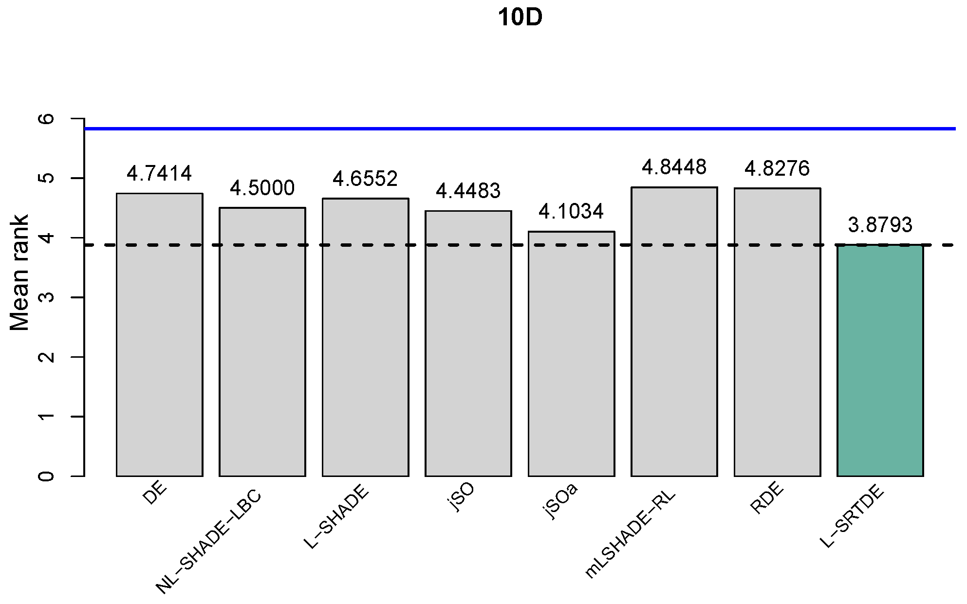
In
Figure 1,
Figure 2,
Figure 3 and
Figure 4, a critical distance indicates that there exists a statistical difference among the two compared algorithms if the difference between their Friedman rank values is smaller than the critical value. We plot a dotted line of the best-obtained algorithm and the blue line to show the critical distance compared to the best-performed algorithm, which is depicted in green.
Figure 1 shows the comparison for
, and we can see that all eight algorithms are below the critical distance from L-SRTDE, which is the best algorithm. This means there are no significant differences between all eight algorithms.
Table 12 tabulates Friedman ranks, shows a performance order in the Rank column, and at the bottom of the table, the
and
p values of the Friedman test are reported. If the
p-value is lower than predefined significance level (
), it indicates that the algorithms have statistically significant differences in performance.
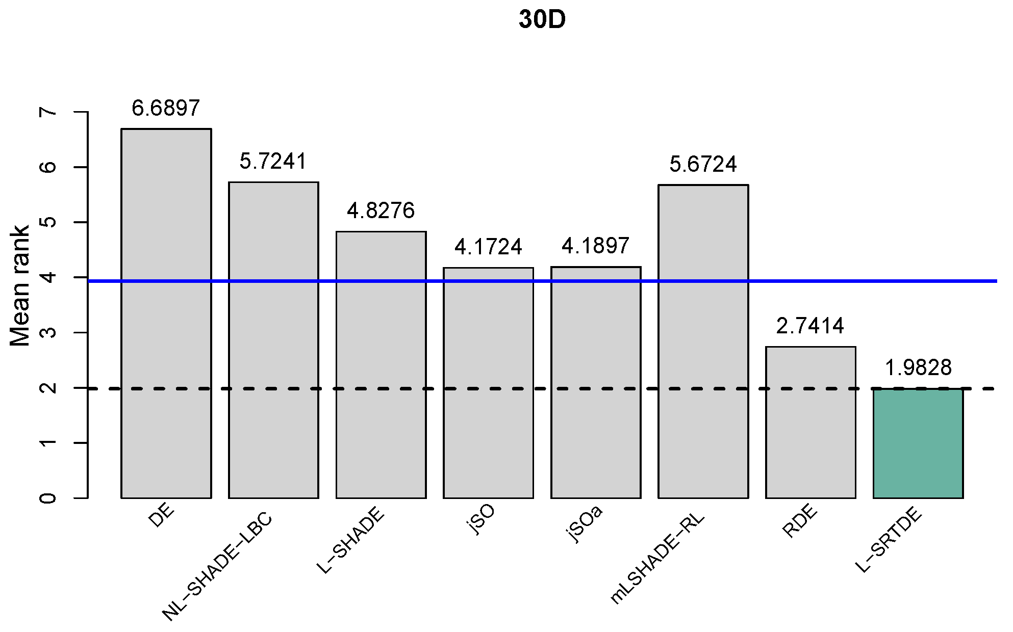
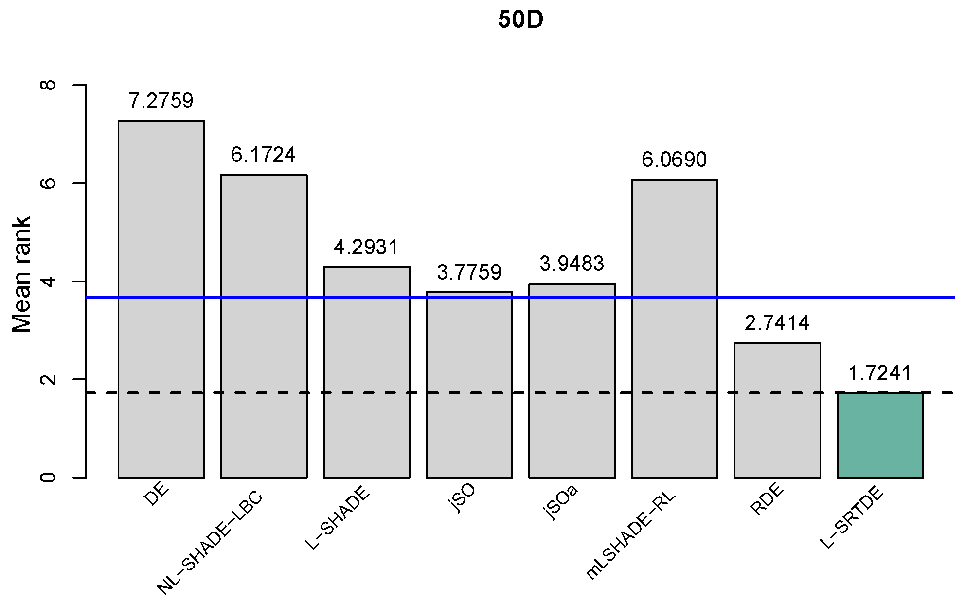
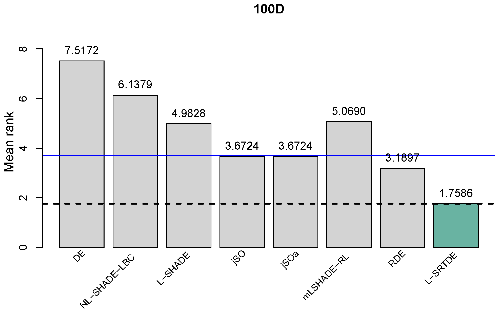
The obtained results for
,
, and
are shown in
Figure 2,
Figure 3 and
Figure 4, respectively. One can see that L-SRTDE is statistically better than DE, L-SHADE, NL-SHADE-LBC, jSO, jSOa, and mLSHADE-RL, while there is no statistical difference between L-SRTDE and RDE. This holds for each dimension of
,
, and
.
On , we can also see that algorithms RDE, jSOa, and jSO are close to the blue line (i.e., critical distance), and RDE is the only one that is slightly below the blue line.
In general, all three tests that were used in the comparison of the eight algorithms report very consistent comparison results for each dimension.
7. Discussion
The classic DE algorithm lacks the sophisticated mechanisms introduced in the algorithms, which were proposed later. While it is generally effective, it struggles with maintaining diversity and balancing exploration and exploitation without additional enhancements. It does not have adaptive mechanisms for F and , leading to suboptimal parameter tuning. It does not have an external archive or hybrid strategies, limiting diversity control. It does not use a restart mechanism, making it prone to premature convergence.
The ranking of the compared algorithms reflects each algorithm’s ability to balance exploration and exploitation, maintain population diversity, and adapt to different stages of evolution. L-SRTDE leads due to its success rate-driven adaptation, refining both mutation and scaling. The repaired crossover rate () refines the crossover mechanism, ensuring more effective variation across dimensions. RDE follows closely, leveraging hybrid strategies and adaptive resource allocation. It combine “DE/current-to-pbest/1” and “DE/current-to-order-pbest/1”. The key improvement is in how resources are allocated between these strategies—an adaptive mechanism evaluates their average fitness improvement and adjusts accordingly. Additionally, RDE incorporates rank pressure-based selection, refining the probability of selecting individuals based on fitness ranks. jSOa stands out for its archive management, ensuring stability. Instead of randomly deleting older solutions, jSOa divides the archive into “better” and “worse” sections based on functional values. This ensures that stronger solutions are preserved while allowing some weaker solutions to be refreshed. This more structured archive update leads to better diversity retention without compromising convergence speed. jSO remains strong, though jSOa refines its archive. mLSHADE-RL’s multi-operator approach seems to be powerful. Non-linear population size reduction strategy combined with linear bias change for both the scaling factor F and the crossover rate improve the efficiency of the NL-SHADE-LBC algorithm. The L-SHADE algorithm, with its robust adaptive mechanism and dynamic population control, serves as the basis for many enhancements to the DE algorithm.
Each of these algorithms offers unique strengths, but L-SRTDE currently represents the most advanced evolutionary strategy in this group of algorithms.
8. Conclusions
In this study, we conducted a comprehensive review of state-of-the-art algorithms based on Differential Evolution (DE) that have been proposed in recent years, including L-SHADE, jSO, jSOa, NL-SHADE-LBC, mLSHADE-RL, RDE, and L-SRTDE, along with classic DE. We examined the key mechanisms incorporated into these algorithms and systematically compared their performance. Specifically, we identified shared and unique mechanisms among the algorithms.
To ensure robust performance evaluation, we employed statistical comparisons, which provide reliable insights into algorithm efficacy. The Wilcoxon signed-rank test was utilized for pairwise comparisons, while the Friedman test was applied for multiple comparisons. Additionally, the Mann–Whitney U-score test was incorporated to enhance the statistical rigor of our analysis. We also performed a cumulative assessment of the eight algorithms and evaluated their performance across different function families, including unimodal, multimodal, hybrid, and composition functions.
The experimental evaluation was conducted on benchmark problems defined for the CEC’24 Special Session and Competition on Single Objective Real Parameter Numerical Optimization. We analyzed problem dimensions of 10, 30, 50, and 100, running all algorithms independently with parameter settings as recommended by the original authors.
The key findings from our experiments indicate that all three statistical tests consistently ranked the algorithms in the following order: L-SRTDE achieved the highest rank, followed by RDE. Next are jSOa and jSO, which alternate between third and fourth positions. LSHADE consistently follows in fifth, succeeded by mLSHADE-RL and NL-SHADE-LBC, with DE ranking last. Notably, a similar ranking was obtained by the method proposed in [
8], which was also employed for algorithm ranking in CEC 2024 [
34]. However, the CEC 2024 competition was performed only at dimension
[
34]. We extend the analysis to a lower dimension (
) and higher dimensions (
and
). The analysis across different function families ranks the algorithms slightly differently at dimension
; however, at
, L-SRTDE remains the best across all function families.
In conclusion, significant progress has been made since the first published Differential Evolution algorithm. The enhanced versions of DE now incorporate a variety of mechanisms, all of which collectively contribute to improved performance.


