1. Introduction
In recent years, deep learning (DL) has significantly impacted various industrial sectors, achieving remarkable success in fields such as image processing and natural language (or audio) processing. Moreover, in relatively less-explored industrial domains like prognostics and health management (PHM), DL has demonstrated promising results. PHM refers to the process of monitoring, analyzing, and predicting the health and performance of equipment and machinery. PHM systems aim to detect potential failures before they occur by assessing the condition of assets through various sensors and data analysis techniques. This helps optimize maintenance schedules, reduce downtime, and extend equipment lifespan. The ultimate goal of PHM is to enhance the reliability and efficiency of industrial operations by predicting failures, improving safety, and minimizing costs associated with unplanned maintenance and repairs. Additionally, synthesizing explanations for machinery experts [
1] and aiding decision-making processes for domain experts [
2] are equally critical.
The economic significance of predictive health monitoring (PHM) has been increasingly recognized across industrial sectors. Recent studies highlight substantial financial benefits, showing that organizations implementing PHM technologies experience significant reductions in maintenance costs and operational downtime [
3].
1.1. Prognostics and Health Management
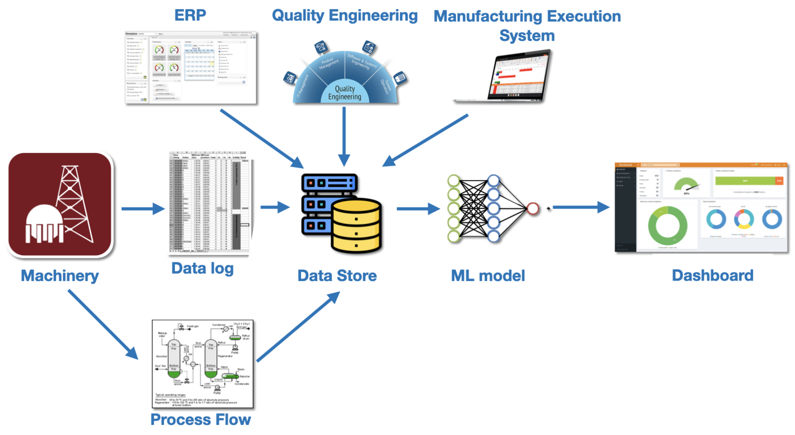
Predictive health monitoring (PHM) systems represent an advanced integration of sensing technologies, data analytics, and machine learning. The diagram in
Figure 1 illustrates the workflow of a PHM system, specifically for predictive maintenance in an industrial setting.
The process begins with industrial machinery as the primary source of operational data, equipped with sensors that continuously monitor performance and health metrics. Raw sensor data—such as temperature, pressure, and vibration levels—are logged and recorded. A process flowchart outlines the machinery’s role within industrial operations, providing insights into interactions and potential failure points. All collected data, including sensor readings and process flow information, are stored in a centralized repository to ensure efficient aggregation and availability for analysis.
The three upper-level components represent industrial support systems. The ERP (enterprise resource planning) system manages core business processes, optimizing inventory, orders, and maintenance using stored data. Quality engineering applies quality management principles, analyzing data to ensure machinery meets standards and implementing improvements. The manufacturing execution system (MES) monitors and controls production in real time, adjusting processes to enhance efficiency and minimize downtime.
The AI core is the ML models which are applied to the stored data to predict future machinery failures before they occur. These models analyze patterns and anomalies in the data to identify potential issues that might lead to equipment failure. The results from the ML models are visualized in a user-friendly dashboard, providing real-time insights into the health and performance of the machinery, highlighting areas that need attention and predicting future maintenance needs. It includes various metrics and KPIs (key performance indicators) that help in decision making.
Data-driven methods have gained popularity for their ability to leverage vast amounts of data from modern sensors and systems (e.g., the Internet of Things). These methods process historical data to identify patterns and detect degradation trends. Various approaches have been explored, including neural networks [
4], deep learning [
5], XAI [
1], and ensemble methods based on decision trees [
6,
7]. Support vector machines (SVMs) have also been applied to RUL in studies such as [
8,
9]. To address uncertainty, Bayesian networks [
10] and fuzzy logic-based systems [
11] have been proposed, enhancing the robustness of RUL predictions.
1.2. Neural Architecture Search
The design of neural architectures is a critical factor in extracting task-relevant features, significantly impacting the performance of the resulting model. Over the course of neural network research, various high-level architectures have been introduced, including feedforward networks (FFNs), convolutional neural networks (CNNs), recurrent neural networks (RNNs), and Transformers, among others. Nevertheless, identifying the optimal hyperparameter configuration—such as the number and types of layers, activation functions, number of neurons, learning rate, and other related parameters—remains a challenging task that requires substantial expertise and iterative fine-tuning.
Neural architecture search (NAS) is an emerging approach in the automated design of neural networks, aiming to systematically identify the optimal network architecture for a specific task. This paradigm explores various network structures to determine which one delivers the best performance, optimizing both accuracy and resource efficiency.
Three key components define NAS. Firstly, at its core is the architecture search space, which encompasses all possible network configurations that can be evaluated for a given problem. Secondly, the evaluation process plays a critical role in determining which architecture best meets the requirements, such as prediction accuracy or computational efficiency. Lastly, to find the optimal architecture, NAS employs optimization methods that guide the search, using techniques such as evolutionary algorithms or reinforcement learning. In this way, NAS enables the automation and substantial improvement of neural network design, reducing the need for manual intervention in selecting parameters and structures.
In machine learning (ML) practices, NAS is typically structured with an outer loop that searches for optimal network hyperparameters and an inner loop that optimizes the model parameters (i.e., the network weights) using those hyperparameters. This work focuses on implementing early-stopping mechanisms within the inner loop to improve efficiency in NAS.
NAS typically requires training and evaluating a large number of candidate models—often in the hundreds—throughout the search process. This makes NAS inherently resource-intensive and time-consuming. For instance, in [
12], Zoph et al. introduce NASNet, which requires 2000 GPU days to perform a search using reinforcement learning, while AmoebaNet-A, presented by Real et al. in [
13], demands 3150 GPU days using evolutionary algorithms. Consequently, developing strategies to reduce the computational resources and time required for NAS is of paramount importance, enabling broader accessibility and greater efficiency in deploying NAS-based methodologies.
NAS faces several computational and methodological challenges. One key challenge is combinatorial complexity, as the architecture search space grows exponentially with the depth and width of the network. This makes finding the optimal architecture increasingly difficult as the design space expands. Another significant hurdle is computational cost, as evaluating multiple architectures requires substantial resources in both time and hardware. Additionally, transferability poses a challenge, as optimal architectures may vary across different domains, meaning that a network architecture effective for one task may not perform as well in another. Finally, interpretability remains a major issue, as understanding why one architecture outperforms another is often not straightforward, making it difficult to gain insights into the factors driving performance differences.
NAS for PHM
While the general principles of NAS are universal, their application in specific domains like prognostics and health management (PHM) requires important adaptations.
Interpretability constraints, reliability requirements, handling of limited or noisy data, and the need for explainability all come into play. The transition from generic NAS to NAS specialized for PHM involves addressing these unique domain-specific constraints. In PHM, ensuring that the system can explain its predictions and operate reliably under uncertain conditions is particularly important. Additionally, the limited availability of clean data in many PHM scenarios adds complexity to the design process, necessitating methods that perform well even with noisy or incomplete information [
14].
While NAS provides a framework for automating model design, accurately estimating the potential performance of a model with minimal computational resources remains a significant challenge. This issue is especially critical in domains like PHM, where both computational efficiency and predictive accuracy are crucial. Our approach aims to develop a learning-curve estimation technique that provides early, reliable insights into the potential performance of a model, thereby minimizing the computational overhead typically associated with traditional NAS methods [
15].
1.3. On Estimating Learning Curves from Initial Data
In the study of neural networks (and ML in general), analyzing the mathematical properties of learning curves is of significant important. These curves, which track the evolution of error or loss during training, provide valuable insights into model convergence and overall behavior.
Key properties of learning curves that offer critical insights into the behavior of DL models and guide more effective training strategies include [
16] the following:
Convergence rate: The speed at which error decreases during training iterations, reflecting the optimization efficiency of the process.
Smoothness: The degree of regularity or stability in learning curves. Smoother curves often indicate more stable and predictable training processes.
Convexity: Whether learning curves exhibit convex behavior, which simplifies analysis and optimization.
Notably, these factors facilitate the study of the initial curvature of learning curves, which may contain predictive information about a model’s final performance [
17]. A steeper initial curvature, representing a rapid decrease in error, could indicate better final performance. Investigating the relationship between initial learning curve curvature and final performance across various neural network architectures and datasets is therefore a promising area of research.
This subsection does not aim to comprehensively address the foundational problem [
16,
17]. Instead, it focuses on leveraging initial behavior (early stopping) to predict future performance and identify the best model. Typical methods for fitting learning curves involve cross-validation or direct parameter tuning to extrapolate performance to unseen dataset sizes. Parametric approaches, such as modeling loss functions with exponential or power-law behaviors, are particularly useful in ML settings where data complexity varies widely [
16]. These approaches form the basis of the practical estimation strategies explored here. We briefly discuss other approaches, along with their advantages and disadvantages, which justify further exploration of alternative solutions.
1.3.1. Extrapolation of Learning Curves
In the ML literature, the term “learning curve” is understood in two different ways. The first, more general, meaning refers to the learning curve as a function of the size of the training set. These types of learning curves have been studied to extrapolate performance from smaller to larger datasets and are not the focus of this paper. The second, more commonly used, meaning refers to the learning curve as a function of the number of training iterations (neural network epochs in this work).
In this paper, we consider the learning curve , where represents the loss function of the model applied to the dataset x with parameters at epoch t.
An intuitive approach to predicting learning curves is based on the method proposed by Domhan et al. [
18], which considers a family of parametric functions to extrapolate the learning curve
f from its initial observations.
In this framework, the curves are modeled as a weighted linear combination of
k basis functions
, each dependent on time
t and parameter vectors
. The central assumption is that the curve being estimated can be modeled as
where
represents the set of all parameters
, and
w denotes the weight vector associated with the parameters used in the basis functions. The prediction process also assumes observational noise around the unknown true value
, modeled as
where a prior is defined for the parameters. Using a gradient-free Markov chain Monte Carlo (MCMC) method, samples from the posterior distribution are obtained to predict future values of the learning curve.
The approach is flexible due to the inclusion of arbitrary parametric functions, allowing it to adapt to various neural network architectures and hyperparameter configurations. However, a key limitation is that the model does not leverage previously evaluated hyperparameter configurations, requiring observation of a significant portion of the learning curve before its predictions become reliable.
A crucial aspect of this methodology is estimating the curvature of the learning curve to predict its future behavior, such as detecting convexity. Using the central limit theorem, the distribution of sample means approaches normality for sufficiently large sample sizes. Therefore, to estimate the curvature,
S independent experiments are performed, generating predictions for large enough epochs
m to reveal reliable trends. This provides a solid foundation for evaluating the progression of the learning curve. For instance, based on Donham’s method, if
is the predicted learning curve
then the curvature of
is
which can provide valuable insights into the evolution of the learning curve. Thus, the curvature depends on the values of
. If the curvature is positive, the curve is convex, which typically indicates that the model is improving its performance at an increasing rate. Conversely, a negative curvature (concave) suggests that the improvement rate is slowing down, often signaling that the model performance is stabilizing.
1.3.2. The Power-Law Hypothesis
Before introducing a new method for NAS and its application in the context of PHM, it is crucial to evaluate whether a parametric approach is appropriate. In particular, by using power-law functions.
The answer is not clear-cut. In some cases, parameterizations of power-law functions can be effective, while in others, they may not be applicable. The question of whether learning curves in PHM can be reliably modeled with power laws or require alternative functional forms is fundamental given the complexity of PHM environments. Let us briefly examine this issue.
Taking the curve as in our case (as a function of epochs), several models exist that use a parametric power law to model the learning curve. For instance, Kadra et al. [
19] model learning curves using a neural network ensemble, with the output being conditioned to follow a power law, and [
20] Tissue et al. model the learning curve using a power law but as a function of epochs and learning rate annealing.
Starting from the hypothesis that the learning curve follows a power law (or a parametric sum of such functions),
the problem can be narrowed to estimating the parameters
. These can be effectively inferred through methods like the Domhan approach, as previously described, or via specialized techniques for power-law detection (cf. [
21]). In [
21], Clauset et al. introduce a statistical method to estimate power-law parameters and conduct goodness-of-fit tests using robust techniques, including the Kolmogorov–Smirnov test, to compare power-law fits with alternative distributions.
The utility of power-law models in PHM has been recognized for their generalization capabilities (for instance, in [
22] Hestness et al. show the power-law relation between DL models’ generalization error and factors such as the amount of training data, model size, and compute resources), though alternative functional forms are often needed to capture intricate learning dynamics [
23]. PHM scenarios frequently involve diverse equipment and operational conditions, leading to learning curves that deviate from power-law behavior. For example, exponential functions effectively model rapid initial error reduction in systems with stable signal-to-noise ratios [
18]. Complex PHM systems may also exhibit phase transitions, requiring hybrid or piecewise models over purely parametric approaches. Selecting functional forms should depend on empirical validation, model evaluation, and domain expertise.
1.3.3. Modeling Learning Curves by Stochastic Processes
An alternative approach to modeling learning curves is to harness their stochastic nature. Specifically, consider a stochastic process
, where
represents the loss at time
t (see [
24]). While stochastic processes are widely used in machine learning (e.g., [
25]), the stochasticity here arises from parameter updates at each epoch. In the expression
, the parameter vector
is defined recursively as
, leading to the relationship
Modeling learning curves as stochastic processes offers several advantages. First, it captures the inherent randomness in the learning process, which is influenced by factors such as weight initialization, the order of training data, and noise in the data. Additionally, it allows for the quantification of uncertainty in predicting the final performance of the model, a crucial aspect for informed decision making. Stochastic modeling also provides access to powerful analytical tools from statistics and probability theory, which can be used to study the properties of learning curves and predict future performance.
It is useful to hypothesize that
follows a classic stochastic diffusion process, expressed as a differential stochastic equation of the form
where
is the drift term, representing the deterministic trend of the learning curve;
is the diffusion coefficient, capturing stochastic variability; and lastly
is a standard Brownian motion. This kind of stochastic differential equations has been extensively studied. For example, Brogat-Motte et al. [
26] present a method for estimating both the drift and diffusion coefficients of continuous, multidimensional, nonlinear stochastic differential equations (SDEs) that are influenced by control inputs.
Our learning-curve estimator
can predict final performance based on
N initial epochs in stochastic terms:
The interest in stochastic modeling lies in the available tools for estimating the learning curve. Using the classical result of Itô [
27], if we model the curve with Equation (
1) and
is twice differentiable in
and differentiable in
t, the change in
is given by
This solution is useful for stochastic modeling of learning curves. For example, using for , we would obtain a stochastic expression for the curvature of .
Integrating both sides of the lemma of Itô, we obtain
Substituting
with Equation (
1) in the second integral term, we obtain
This integral form of the lemma is useful for evaluating at the final time T, based on its initial value and the integral contributions over time. For , as in our case, it provides a detailed estimation.
Despite its benefits, stochastic modeling of learning curves comes with some limitations. One key challenge is complexity: some stochastic models can be intricate and difficult to fit to the available data. Furthermore, these models rely on assumptions about the learning process that may not always be valid, which can affect their accuracy in certain contexts. Lastly, stochastic models require a sufficient amount of data to accurately estimate their parameters, posing a problem in situations where data are limited.
1.4. Bayesian Optimization for Neural Architecture Search
In the optimization process described above, the input to the objective function f consists of the model architecture and training hyperparameters, while the output is the performance of the model trained with the given settings. Bayesian optimization (BO) is particularly effective in scenarios where evaluating f is computationally expensive.
The BO framework provides a probabilistic approach to optimizing expensive-to-evaluate objective functions, especially when the function lacks a known analytical form or is computationally demanding. BO uses a surrogate model, typically a Gaussian process, to approximate the objective function based on prior evaluations. An acquisition function then guides the selection of the next evaluation point, balancing exploration of uncertain regions with exploitation of promising areas. This iterative approach makes BO highly efficient, requiring significantly fewer evaluations compared to brute-force or grid-search methods. BO is widely applied in hyperparameter optimization, NAS, and experimental design. For instance, in [
28], Kandasamy et al. present NASBOT, a BO framework for NAS using a novel distance metric, in the space of neural network architectures.
A typical application of BO in ML involves model selection tasks [
29], where the generalization performance of a statistical model cannot be determined analytically and must instead be evaluated empirically. For example, BO can be used to select the parameter
and the kernel bandwidth
h for SVMs.
Methods based on BO provide a systematic and automated alternative to traditional practices commonly employed in PHM. Typically, human experts inspect learning curves during training to identify and terminate runs with poor hyperparameter settings, thereby accelerating manual hyperparameter optimization. In PHM, learning curves play a central role in evaluating the performance of algorithms with respect to resources such as the number of training examples or iterations [
17]. These curves have a variety of applications, including guiding data acquisition strategies, implementing early-stopping criteria to prevent overfitting, and facilitating model selection processes [
18]. BO enhances these tasks by automating the exploration and optimization of hyperparameters, reducing the need for manual intervention while maintaining efficiency.
1.5. Aim of the Paper
This work focuses on leveraging learning curves to eliminate unpromising models early in the NAS process using BO. Building on prior research [
30], the present work aims to optimize NAS specifically for PHM applications by introducing a novel performance estimation framework. This framework is designed to streamline the NAS process by significantly reducing computational costs while maintaining high-quality model selection.
The core of the proposed approach lies in an intelligent estimator capable of predicting the long-term performance of a model by analyzing only a few initial training and validation epochs. To achieve this, the estimator is built using an extensive dataset comprising 62 predictive maintenance problems, ensuring its robustness and generalization. This estimator is then seamlessly integrated into the BO loop, enabling the process to efficiently prune unpromising candidates and allocate resources to models with higher potential, thereby enhancing the overall efficiency of NAS in PHM tasks.
In our proposed model, prior assumptions about the functional form of the curves are not required. While such assumptions could simplify the problem, they are not necessary within our framework. As a result, our method generalizes beyond purely parametric approaches, making it better suited to environments characterized by heterogeneity, such as in the context of PHM.
1.6. Structure of the Paper
This work is structured as follows.
Section 2 presents some related works, where key developments and methodologies related to the proposed approach are discussed.
Section 3 provides the foundations of Bayesian optimization, offering an introduction to the technique, whereas Section Bayesian Optimization Based on a Gaussian Process elaborates on Bayesian optimization, explaining its integration with Gaussian processes.
In
Section 4, the datasets used in this study are described in detail, focusing on their characteristics and applicability to predictive maintenance tasks.
Section 5 outlines the main approach and methodology developed in this work.
Section 6 details the architectures of the performance estimators used in the study and the training procedure. Finally, the performance of the estimators is assessed and analyzed under different conditions.
In
Section 7, the early-stopping methodology applied during BO-based NAS is discussed. This section defines the metrics used to evaluate the performance of the early-stopping process, presents the results obtained, and compares the approach with different baselines.
Section 8 is devoted to conducting a theoretical analysis of two fundamental aspects of the method. Firstly, the impact of additive and autoregressive noise on learning curves and early-stopping efficiency is investigated. Secondly, the convergence of robust early-stopping methods under noise is analyzed.
Finally,
Section 9 contains a discussion of the results and insights obtained from the experiments and theoretical analysis, and
Section 10 concludes the work, summarizing the findings and suggesting potential directions for future research.
2. Related Work
Building upon the ideas introduced in the Domhan et al. paper [
18] mentioned above, Baker et al. propose a method for enabling early stopping during the training of neural networks by leveraging learning curves [
31]. This method employs an estimator to predict the final performance of a model during its training. If the estimated performance is lower than the best performance observed so far, the training process for that model is terminated prematurely. This early-stopping approach is integrated into the Hyperband optimization algorithm [
32], which is designed to efficiently allocate computational resources during hyperparameter optimization. Furthermore, Klein et al. [
17] explore the use of Bayesian networks for modeling learning curves within the Hyperband framework, enhancing its predictive capabilities during hyperparameter search.
It is important to highlight that the Hyperband algorithm operates as a resource allocation strategy and does not utilize performance data from previous iterations when selecting new configurations to evaluate. Instead, Hyperband accelerates random search by applying an adaptive early-stopping mechanism that dynamically allocates resources—such as training iterations, data samples, or features—based on intermediate performance metrics.
Within the context of Bayesian optimization (BO), various methods have been developed to improve efficiency by incorporating early-stopping mechanisms. These methods aim to halt evaluations of unpromising hyperparameter configurations within the inner loop of the optimization process. A notable example is BOHB [
33], which combines the strengths of Bayesian optimization and Hyperband. BOHB leverages information from previously sampled configurations to guide the search process while retaining the early-stopping strategy of Hyperband to discard unpromising candidates, thereby improving both computational efficiency and solution quality.
Dai et al. [
34] proposed a Bayesian model to estimate the convergence of a model being trained during a Bayesian optimization (BO) iteration. This estimation allowed for the early termination of training, thereby reducing the number of unnecessary training epochs. However, a limitation of this method is that models with limited potential to outperform the current best configuration could still undergo a substantial number of training epochs before being halted.
The field of learning curve prediction and neural architecture search has seen significant developments in recent years, with researchers exploring various approaches to improve computational efficiency and model performance.
Adriaensen et al. [
35] proposed an approach for efficient Bayesian learning curve extrapolation using prior-data-fitted networks. While sharing our goal of improving learning curve prediction, their method focuses primarily on extrapolation techniques, whereas our work emphasizes early stopping in neural architecture search specifically applied in predictive maintenance domains. Their probabilistic modeling approach differs from our more comprehensive framework that studies network hyperparameter information and provides a detailed theoretical analysis of noise in learning processes.
The work by Egele et al. [
36] introduced a provocative method for early discarding of models after just one epoch of training. Their approach is notably simpler compared to our method, focusing on empirical observations rather than a comprehensive theoretical framework. While both works aim to reduce computational costs in hyperparameter optimization, our approach provides a more nuanced estimation process that leverages learning curve characteristics and incorporates domain-specific insights from predictive maintenance. Furthermore, we evaluate the performance of our method using only two observed epochs, making it directly comparable to their approach.
Rakotoarison et al. [
37] developed an in-context freeze–thaw Bayesian optimization technique. Their work shares our interest in Bayesian optimization and computational efficiency, but differs in its primary focus. While they explore a flexible model freezing/unfreezing strategy, our research concentrates on developing a robust performance estimator specifically tailored to learning curve analysis in predictive maintenance contexts.
The foundational work by Klein et al. [
17] on learning curve prediction using Bayesian neural networks laid crucial groundwork in the field. Their pioneering research introduced the idea of using probabilistic models to predict model performance, an approach we extend and refine. Unlike their work, our method incorporates a more sophisticated analysis of noise in learning processes and provides a more comprehensive framework for early stopping in neural architecture search.
Ruhkopf et al. [
38] introduced MASIF, a meta-learning approach for algorithm selection using implicit fidelity information. Although their work shares our interest in meta-learning and algorithm optimization, our research is more specifically focused on learning-curve estimation and early stopping in neural architecture search for predictive maintenance.
Our work distinguishes itself through several key contributions. First, we provide a comprehensive integration of hyperparameter information into the performance estimation process. Second, our approach is specifically tailored to predictive maintenance domains, utilizing a set of 62 different PHM-related datasets. Third, we offer a detailed theoretical analysis of (some models of) noise in learning processes, going beyond previous empirical approaches. Finally, our early-stopping method, based on a sophisticated estimator, provides a more nuanced approach to reducing computational costs in neural architecture search.
3. Background: Gaussian Processes
One approach to studying the learning curve is to model it as a Gaussian process (GP). A GP is a collection of random variables where any finite subset of these variables has a joint distribution that is a multivariate normal distribution. In simpler terms, a Gaussian process defines a distribution over functions, allowing for flexible and non-parametric modeling and predictions for complex data.
Formally, a Gaussian process can be defined as
where
Such that for any finite set of points
, the vector of values
follows a multivariate Gaussian distribution:
where
;
is the covariance matrix, with entries .
Therefore, GPs are characterized by their mean and covariance functions (kernels). As distributions over functions, GPs are highly useful in non-parametric regression, allowing inferences about the behavior of a function without requiring its form to be specified in advance. In machine learning, GPs play a key role in Bayesian optimization (BO), enabling the efficient selection of evaluation points in scenarios where the objective function is costly to compute. By effectively modeling uncertainty, GPs minimize the number of evaluations needed, optimizing both computational resources and time.
Bayesian Optimization Based on a Gaussian Process
Bayesian optimization (BO) is an effective technique for optimizing expensive black-box functions, particularly when evaluations are costly or time-consuming. It is widely used in fields such as machine learning, engineering, and scientific research, especially for tasks like hyperparameter tuning, experimental design, and parameter estimation. BO efficiently balances exploration and exploitation, which is crucial for noisy or multi-modal objective functions. By incorporating prior knowledge through kernel functions, BO is well suited to model complex and unknown landscapes, offering a structured optimization approach with minimal evaluations. While various approaches exist for BO, those based on Gaussian processes (GPs) are the most commonly used in the literature.
Generally, a Bayesian optimization (BO) algorithm operates sequentially: Starting with a Gaussian process (GP) prior for
f at time 0, it incorporates results from previous evaluations at times
to update the posterior for
f. This posterior is then used to construct an acquisition function
, where
measures the value of evaluating
f at
x at time
t (although the function can be independent of epochs). If the goal is to maximize
f, the algorithm selects
as the maximizer of the acquisition function:
Two key elements are necessary for implementing GP-based BO. First, we need a kernel function to quantify the similarity between two points x and in the domain. This kernel is essential for defining the GP, enabling us to reason about the unobserved value when has already been evaluated. Second, we require a method to maximize .
In the context of NAS, the objective function represents the performance of a neural network architecture , where denotes the set of all possible architectures (i.e., the parameter/configuration space). The BO process iteratively searches for the optimal architecture by constructing a probabilistic model of f and using it to guide the search. Formally, the BO process can be described as follows.
Initialization: Begin with an initial set of evaluated architectures , where is the number of initial evaluations.
Probabilistic modeling: Construct a probabilistic model to capture the uncertainty about the objective function f given the observed data . A common choice is a GP.
Acquisition function: Define an acquisition function that quantifies the utility of evaluating a new architecture a, balancing exploration (searching regions with high uncertainty) and exploitation (searching regions with promising performance).
Optimization: Solve the optimization problem to find the next architecture to evaluate. Several optimization techniques, such as gradient-based methods or evolutionary algorithms, can be used.
Evaluation and update: Evaluate the performance of the new architecture and update the dataset .
Iteration: Repeat steps 2–5 until a stopping criterion is met, such as reaching a maximum number of iterations or a target performance level.
Also, local BO has been studied by Wu et al. [
39].
Therefore, the acquisition function guides the search. Common acquisition functions include expected improvement (EI) [
40],
upper confidence bound (UCB)
(which will be used in this paper), and probability of improvement (PI)
.
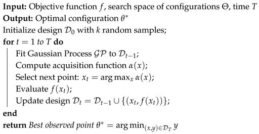
In the case of NAS, the BO algorithm can be formalized as in Algorithm 1.
| Algorithm 1: Bayesian Optimization for Neural Architecture Search |
![Mathematics 13 00555 i001]() |
The BO process is designed with the expectation that as the number of iterations increases it will converge towards the objective with the best value. For example, guiding the method towards minimizing the expected improvement is expected to lead to convergence under the selected strategies (cf. [
41]).
4. Experiments on Predictive Maintenance: Datasets
To illustrate the proposed methodology, a dataset of 61,000 learning curves was generated. This dataset was created using 62 different datasets from multiple tasks in the context of PHM, including failure detection, fault diagnosis, and prognosis. The datasets were obtained using the Python tool
phmd [
42], which facilitates the downloading and loading of each dataset. These datasets were sourced by searching various research repositories, related bibliographies, and the internet. They are public datasets in the context of PHM, covering the years between 2010 and 2022: 10 are provided by NASA [
43,
44,
45,
46,
47,
48,
49,
50,
51,
52], while 8 are offered by the PHM Society through their American, European, and Asian challenges [
53,
54,
55,
56,
57,
58,
59,
60]. Universities worldwide contributed 19 datasets [
61,
62,
63,
64,
65,
66,
67,
68,
69,
70,
71,
72,
73,
74,
75,
76,
77,
78,
79], and 7 more were produced by other research institutions [
80,
81,
82,
83,
84,
85,
86]. One dataset belongs to the Society for Machinery Failure Prevention Technology (MFPT) [
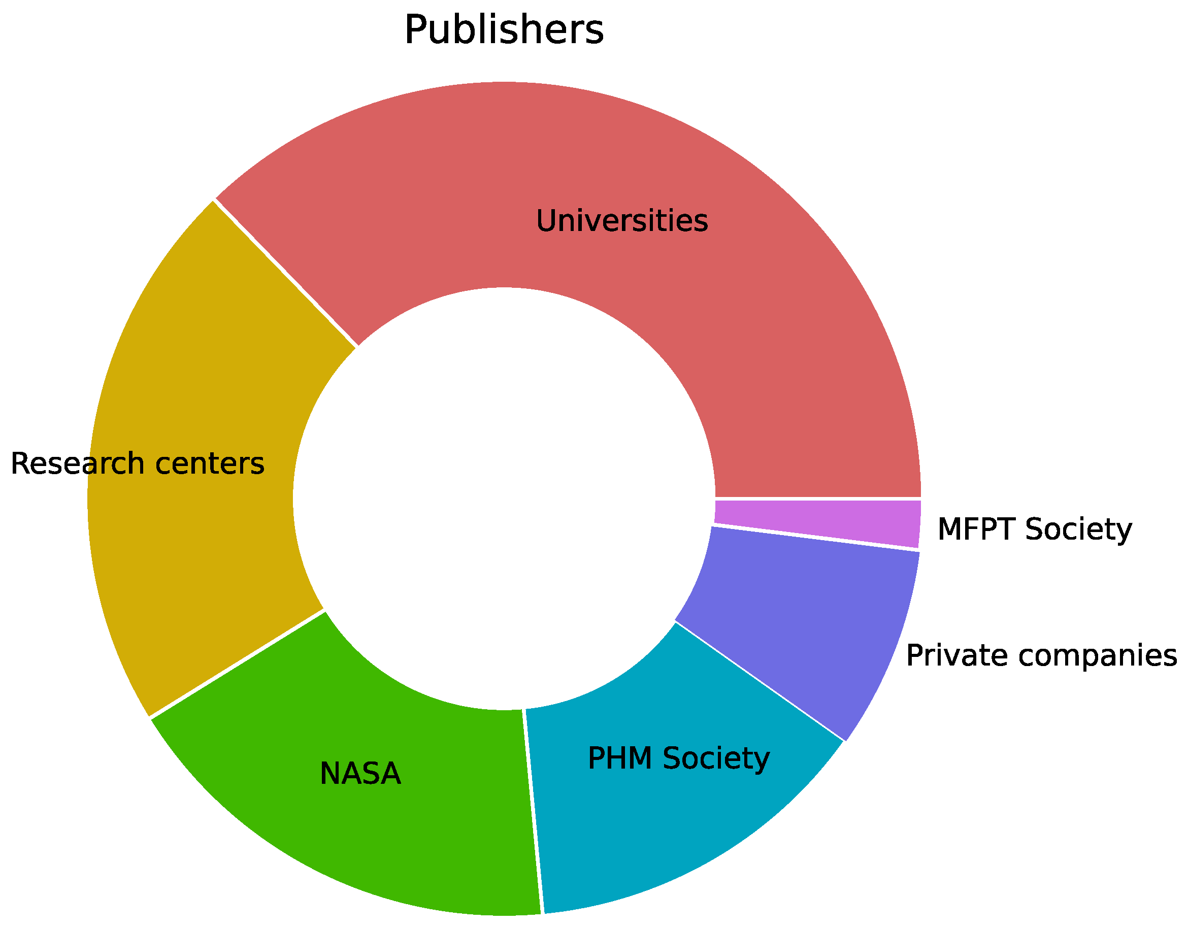
59], and the remaining were published by various companies.
Figure 2 shows the distribution of dataset publishers. Universities, along with research centers, contributed over fifty percent of the datasets. NASA has been treated separately due to its significant contribution to dataset provision over the years. Similarly, the PHM Society, through its annual data challenges, has made a substantial contribution.
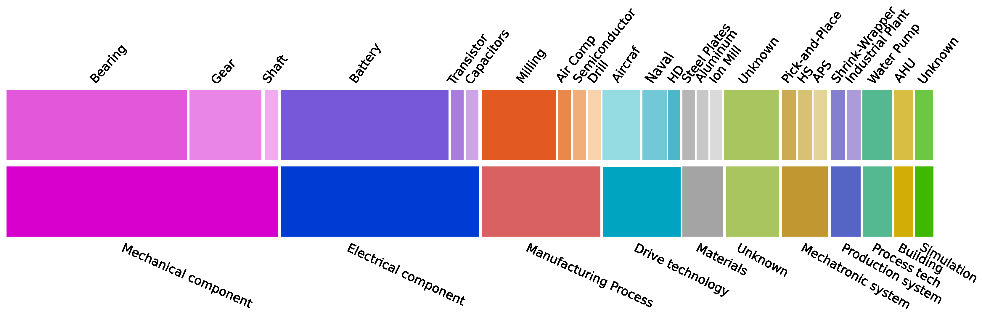
All datasets found were included in the experiment set. The only requirement that a dataset had to meet was that it had to be a time-series dataset. The datasets span multiple engineering domains, systems, and components, such as electrical components, drive technology, mechanical components, and materials, among others.
Regarding the experimental nature of the datasets, the majority of them are categorized under mechanical and electrical component fault diagnosis and prognosis. Within these domains, the analysis of bearings, gears, and batteries predominates.
Figure 3 presents the overall distribution of domains and applications to which each dataset belongs.
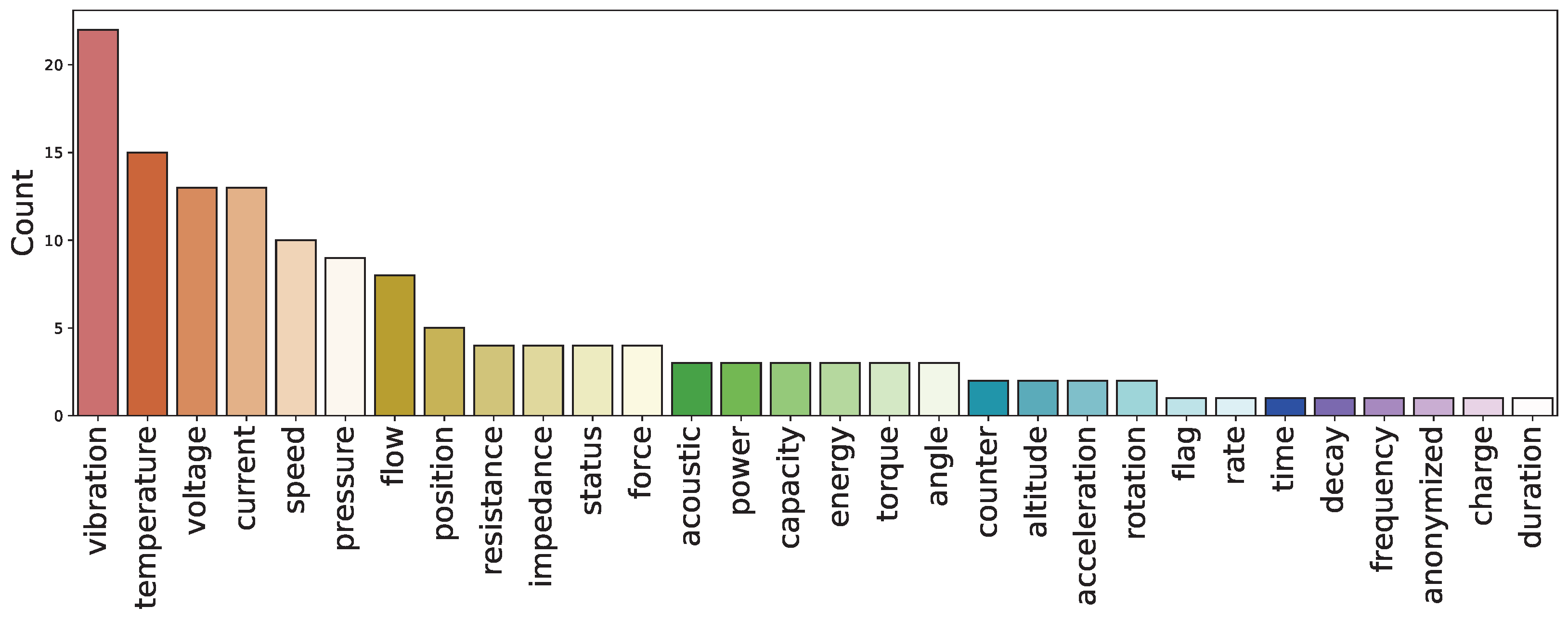
The type of feature present in each dataset has also been categorized, and the distribution is summarized in
Figure 4. As can be observed, there is a high number of vibration features. While generating datasets on mechanical components, accelerometers were used in most cases to measure vibrations; therefore, this kind of feature is very common. Features like temperature, current, and voltage are commonly used in electrical component-based datasets, which are well represented among the datasets gathered.
Figure 5 displays the distribution of modeling tasks and PHM tasks. Regarding the modeling tasks (
Figure 5a), most of the tasks are regression tasks, followed by multiclass classification tasks. Binary classification is less represented and is typically focused on fault detection. Notably, any fault diagnosis task can be converted into a fault detection task by considering the normal or healthy condition as the negative label and the other fault categories as the positive label. In relation to the PHM tasks (
Figure 5b), diagnosis tasks are dominant, followed by prognosis tasks.
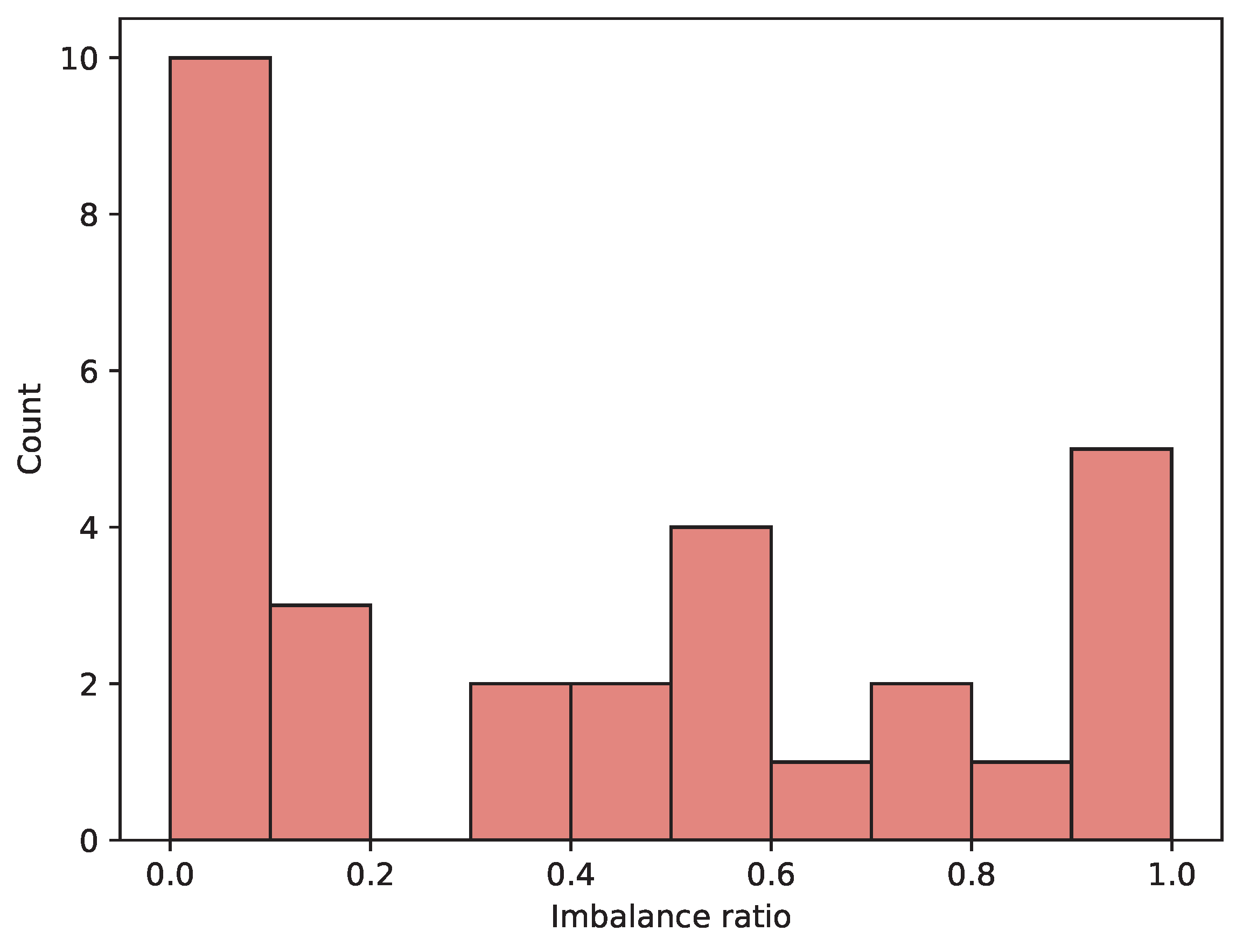
In real-world applications, fault categories are less common than the healthy condition. It is desirable for the set of datasets to be representative of this situation. Therefore, the imbalance ratio of the dataset is an important factor to consider.
Figure 6 shows the distribution of imbalance ratios across the datasets. A considerable number of datasets are imbalanced or very imbalanced, as expected.
For each dataset, neural architecture search (NAS) was performed on four different architectures: Feedforward neural networks (FFNs), deep convolutional networks (DCNs), recurrent neural networks (RNNs), and Transformers.
The NAS process was conducted using Bayesian optimization (BO) implemented using the software published by F. Nogueira [
87]. The Bayesian optimization (BO) algorithm used in our work relies on a Gaussian process (GP) with a radial basis function (RBF) kernel to model the objective function. For selecting the next set of hyperparameters, we employed the upper confidence bound (UCB) acquisition function, with the default hyperparameters
and
. The choice of UCB provides a balance between exploration and exploitation, allowing the algorithm to focus on both areas of high uncertainty and regions where performance is expected to improve.
Each neural architecture search (NAS) run consisted of 100 iterations. The first 20 iterations used random sampling to explore the search space, providing an initial set of diverse observations to seed the GP. Subsequently, the BO process used the UCB acquisition function to guide the search for optimal hyperparameter configurations.
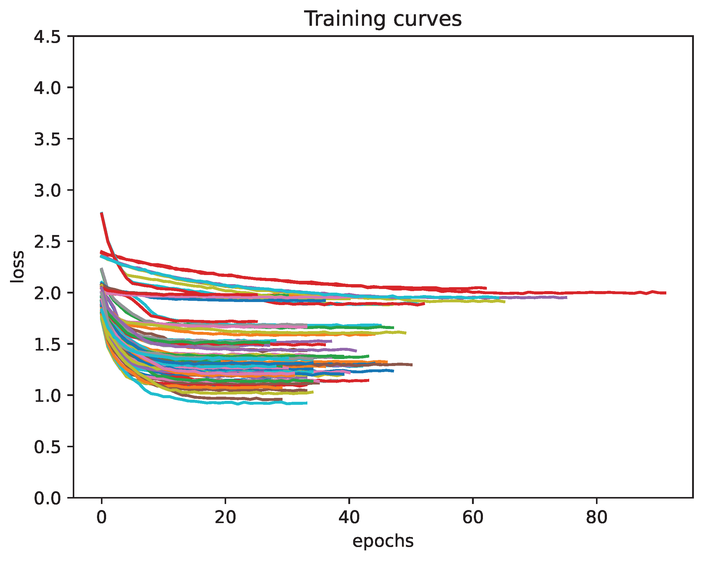
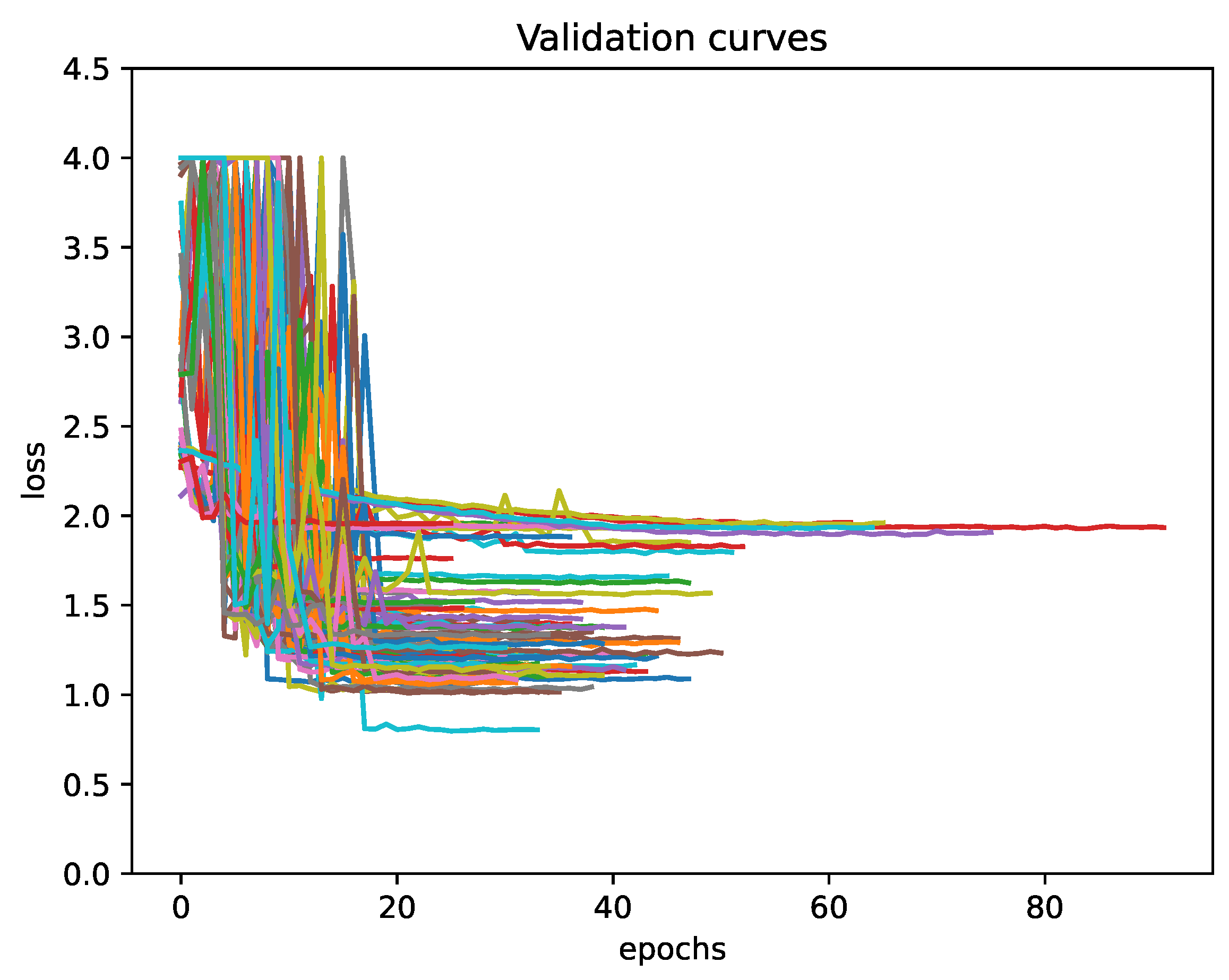
Figure 7 presents a sample of the learning curves generated from the dataset.
5. Overall Description of the Proposal
Our proposal is based on two main components: a learning-curve estimator (
Section 6) and a BO process for NAS that uses the aforementioned estimator for early stopping (
Section 7). Let us briefly describe these elements.
- Learning-curve estimator:
The goal is to develop a model capable of predicting the final performance of a DL model based solely on the first epochs of its training and validation curves. Two versions of the estimator are proposed: An estimator based only on the learning curves, and an estimator conditioned on the hyperparameters of the neural network architecture.
- Integration into BO for NAS:
The learning-curve estimator is used to accelerate the BO process in the search for optimal neural network architectures for PHM tasks. When the estimator predicts that the performance of a model will be significantly worse than the best model found so far, the training of that model is stopped, thus saving computational resources.
The model is trained and evaluated using a dataset of 61,000 learning curves generated from 62 different datasets in the context of PHM, as described in
Section 4.
6. Performance Estimators
The proposed methodology centers on a model designed to estimate the final validation performance of a neural network. This estimation allows for the application of an early-stopping strategy during NAS, improving efficiency and reducing computational costs by halting training early based on predicted performance.
To construct the estimator, the initial step involves selecting a specific machine learning model. The process uses the first N observed points of training and validation performance extracted from the learning curves. These points provide a basis for analyzing and predicting trends by working on pairs of curves: .
The training set to build such a model is composed of a set of former training and validation performances and their corresponding targets. Using the notation
:
where
M is the number of samples in the dataset.
Note that the number of training epochs for each model could be different (see
Figure 7). The variation is due to the models being trained using an early-stopping criterion. This is quite different from other works, where the number of epochs is always the same.
In a second modeling stage, it is studied how the information of the hyperparameters impacts the learning-curve estimator. Thus, the hyperparameters will be included as part of the estimator.
Since the dataset contains various types of architectures and only a general learning-curve estimator is trained, the hyperparameter vector is paired with a one-hot vector that determines whether each hyperparameter is set for that network. Thus, the training set collecting such information for this kind of estimator is of the form
A first approximation to approach the estimation could be to start from
Thus, the approach proposed by Domhan could be applicable. However, as previously mentioned, parameter estimation using MCMC can be computationally expensive, and the most appropriate parametric family (especially in the context of PHM) is unclear. An alternative, which we aim to demonstrate in this paper, is to use a neural network-based model, trained on the available data, to compute
. The architecture of the network is outlined below.
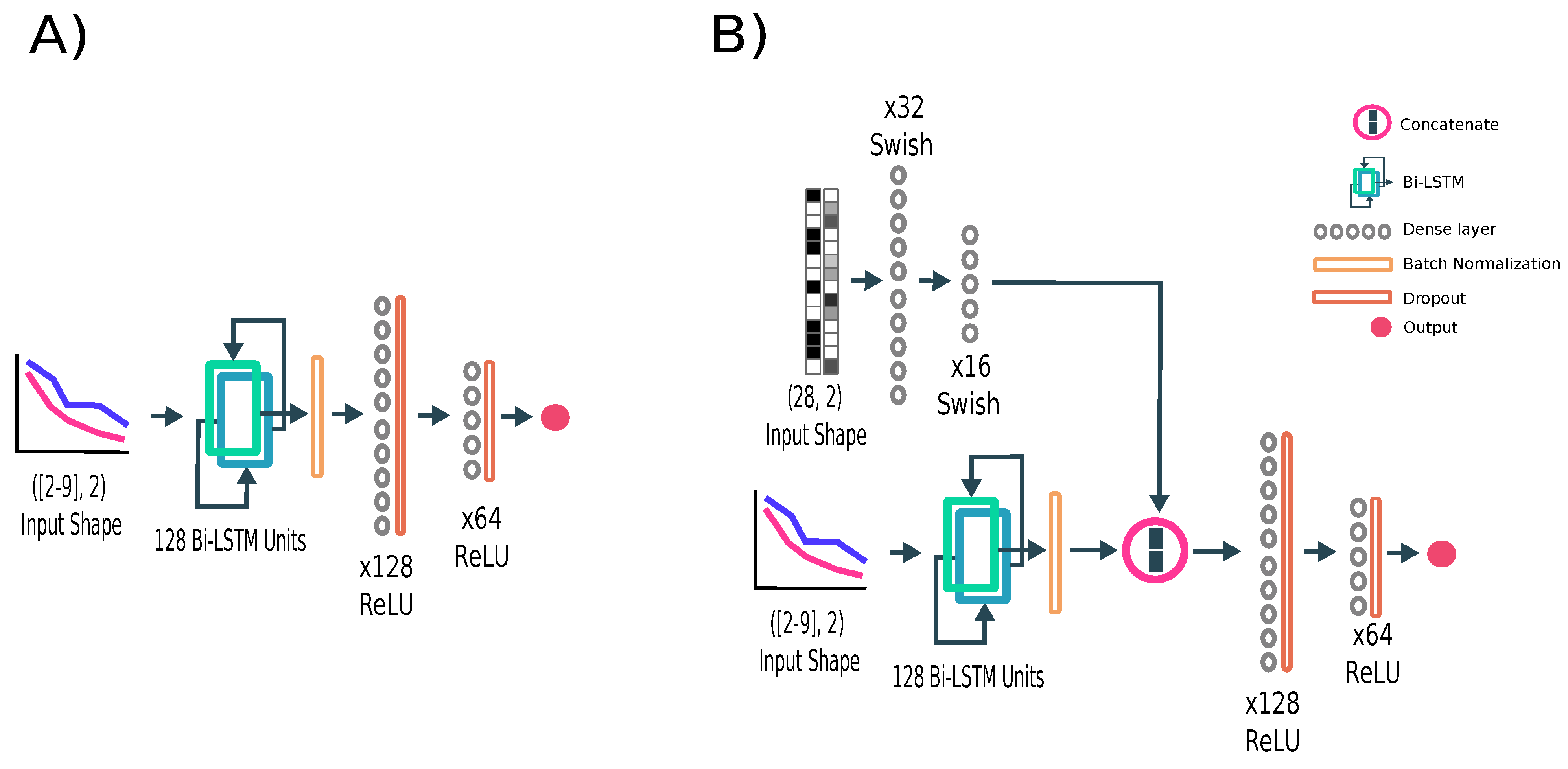
6.1. Performance Estimator Architectures
The selected architecture for the final performance estimator is the LSTM, chosen for its excellent performance in processing and modeling time-series data, effectively capturing both past and future dependencies. The architecture begins with LSTM cells consisting of 128 units. Following these, two fully connected layers with 128 and 64 neurons, respectively, are added, each utilizing ReLU as the activation function. To improve training stability and convergence, batch normalization is applied immediately after the LSTM cells.
The input to the model corresponds to training and validation performance curves, with a variable shape ranging from 2 to 9 observed epochs. The complete architecture is illustrated in
Figure 8.
To analyze the impact of network hyperparameters on the learning process, a conditioned network was designed. The hyperparameters define the architecture of the network responsible for generating the learning curve. Given that the dataset includes different types of networks (FFN, CNN, RNN, and Transformer), certain hyperparameters are not applicable across all architectures (see
Table 1).
To address this, a one-hot vector mask was introduced to indicate the relevance of each of the 28 hyperparameters for a specific network type. Both the hyperparameter vector and the mask, each with dimensions
, are processed through two fully connected layers containing 32 and 16 neurons, respectively. These layers utilize the Swish activation function, defined as
(see
Figure 8B).
The output from the final fully connected layer is concatenated with the output of the Bi-LSTM cells. This combined representation is then passed to the two final dense layers of the network. Detailed summaries of the architectures selected are provided in
Table A1.
6.2. Training Procedure and Estimator Performance
The performance estimators were designed to predict the final validation loss of a network, with the choice of loss function depending on the nature of the task. For regression tasks, the mean squared error (MSE) was used, while classification tasks relied on cross-entropy loss.
The hyperparameters of the performance estimator network to be optimized include the number of LSTM layers, the size of the LSTM cells, the bidirectionality, and the learning rate. To ensure robust training and evaluation, the dataset of performance curves was split at the dataset level (known as group-based splitting) to mitigate overfitting. A total of 30% of the datasets were randomly assigned to the test set, while the remaining 70% were used within a three-fold cross-validation (that is, they were further divided, allocating 66% to the training folds and 33% to the validation fold), to enhance the results’ reliability. Additionally, all experiments were repeated six times with different random seeds to validate the results across diverse test conditions and network initializations.
Table 2 shows the range of hyperparameters studied.
The training process incorporated several optimization techniques to ensure efficiency and stability. Early stopping was applied to terminate training when validation performance failed to improve for eight consecutive epochs, reducing unnecessary computation and minimizing overfitting. A learning rate decay strategy, inspired by the work of You et al. [
88], was also employed. If validation performance showed no improvement for five consecutive epochs, the learning rate was reduced by a factor of 0.1. The Adam optimizer [
89] was used to train the estimators effectively.
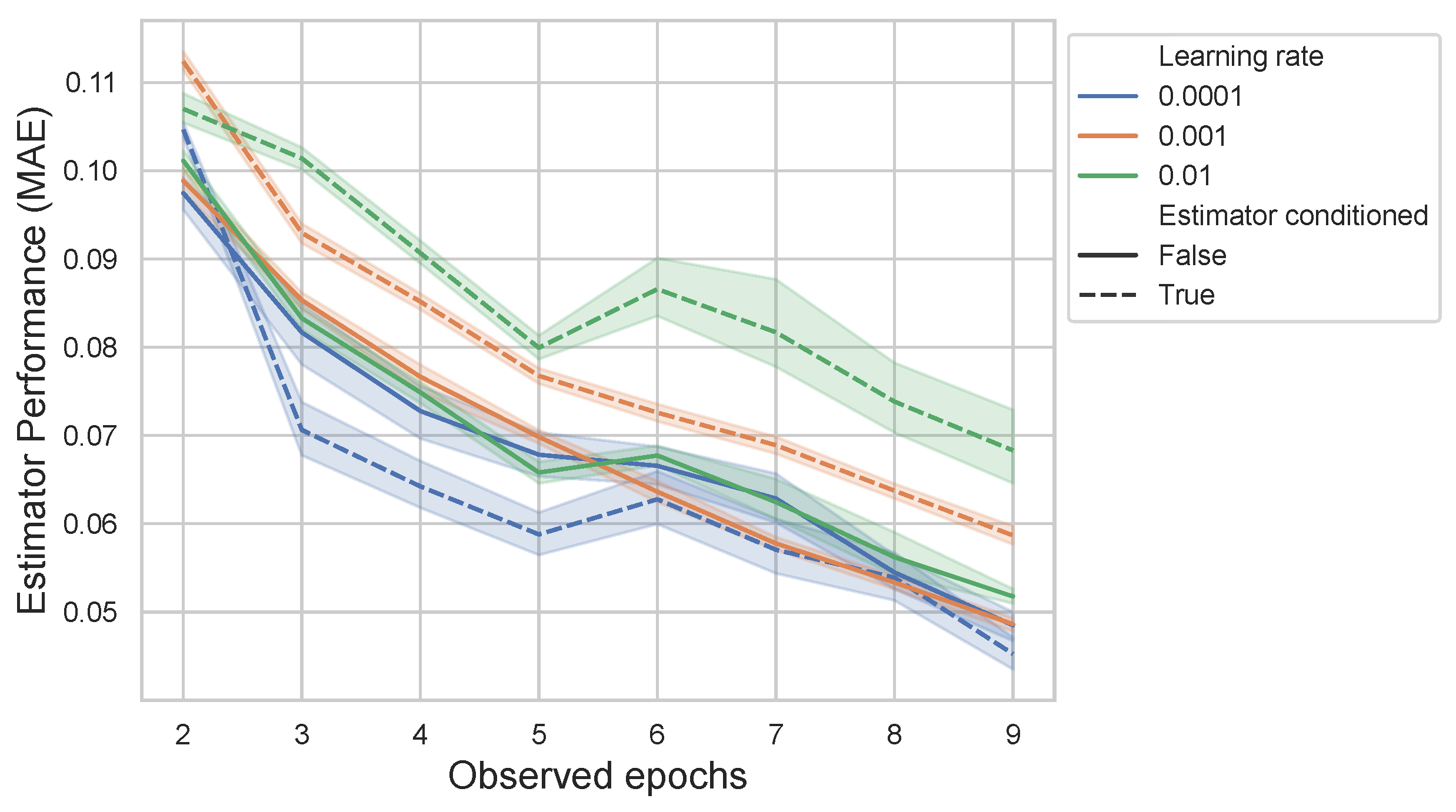
The performance of the estimators, as illustrated in
Figure 9, is influenced by the number of observed training epochs. As anticipated, the estimation error decreases as the number of observed epochs increases, demonstrating the advantage of incorporating more training data. Interestingly, the inclusion of network hyperparameters enhances the accuracy of the estimators, primarily when the number of observed epochs is small. Additionally, the learning rate appears to have a lesser impact on the non-conditional approach, whereas lower learning rates are necessary for the conditional approach to achieve optimal performance.
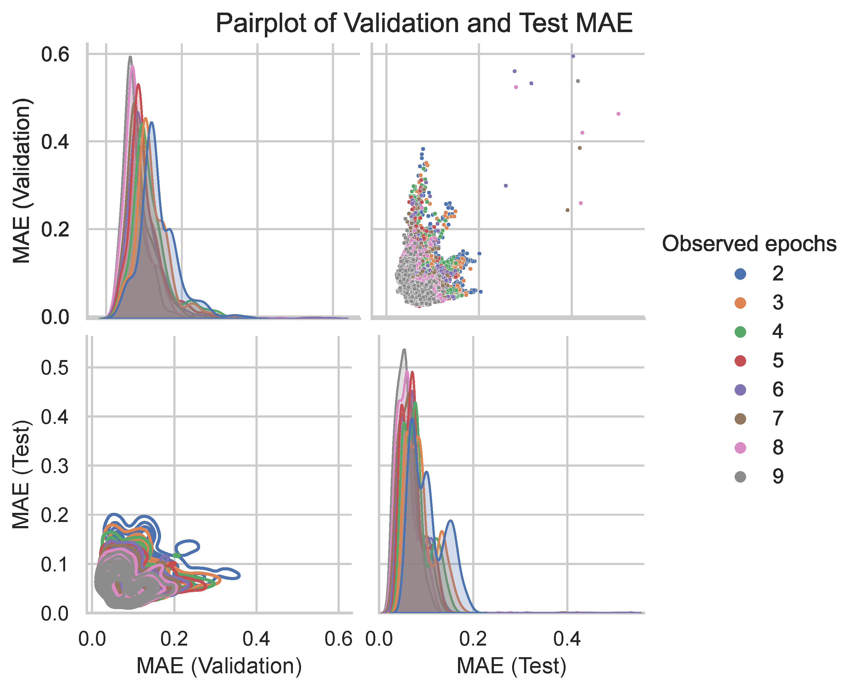
Figure 10 illustrates the relationship between the validation MAE and test MAE as measured by the performance estimator. The figure highlights that a lower number of observed epochs is associated with a reduced likelihood of overfitting, where the model maintains similar performance on both validation and test sets. This trend is particularly evident in the kernel density estimation (KDE) plot, which shows a more consistent alignment between validation and test errors as the number of observed epochs decreases.
6.3. Robustness Analysis
In this section, we analyze the sensitivity of the estimator performance to various hyperparameters using the Sobol sensitivity index. The Sobol index quantifies the contribution of each input parameter to the output variance, providing insight into how robust the model is to changes in hyperparameters. The Sobol index for a given hyperparameter
is computed as follows:
where
Y is the output of the model (e.g., test RMSE) and
is the hyperparameter under study. The numerator measures the variance of the output due to variations in
, while the denominator represents the total variance in the output. The Sobol index values for each hyperparameter are summarized in
Table 3.
For the learning rate, the Sobol index was found to be . This relatively moderate value suggests that the learning rate has a meaningful impact on model performance. Thus, fine-tuning the learning rate is likely to have the most noticeable effect on improving model performance. In contrast, the network depth had a Sobol index of , indicating a small negative influence on the performance of the model. The negative Sobol index suggests that a shallower architecture could be more effective for this problem, and adding extra layers might not contribute positively to performance.
The bidirectional setup yielded a Sobol index of , which indicates a very small positive effect on performance. This suggests that processing information in both forward and backward directions has a minor benefit. Finally, for the number of recurrent units, the Sobol index was , showing a small positive influence on model performance. While this index indicates a modest effect, it still suggests that the width of the recurrent layers plays a role in capturing more complex patterns in the data. However, the contribution is small compared to the learning rate, and adjustments to the recurrent units may lead to marginal improvements rather than drastic changes in performance.
7. Early Stopping During NAS with BO
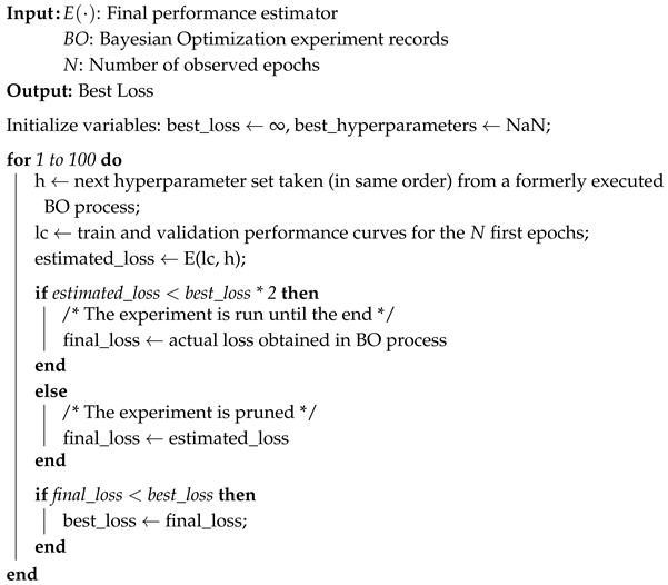
After training the final performance estimator, its effectiveness in reducing the number of epochs required during BO for NAS was evaluated. Since running the BO process across 62 datasets for various architectures is computationally expensive, and these experiments had already been conducted to generate the learning curves, we simulated the BO process using the results from those experiments. Specifically, we followed the same sequence of test set experiments for each dataset as their respective training runs.
The details of this simulation procedure are outlined in Algorithm 2. The condition was introduced as a heuristic rather than a parameter derived from tuning. This threshold was set at the beginning of our study based on the hypothesis that if the predicted loss of a model is twice as high as the best loss observed so far, it is unlikely that the model will outperform the current best. The value of 2 was chosen to provide a balance between filtering out poorly performing models and allowing sufficient exploration. While this specific threshold was not extensively tuned, it reflects an intuitive assumption about the relationship between early loss estimates and final performance. Future work could explore alternative thresholds to better understand their impact on model selection.
7.1. Metrics
Two key metrics were computed to evaluate the impact of early stopping during the BO process. The first metric quantifies the total number of training epochs skipped during the BO process. Early stopping is applied to reduce the computational cost by avoiding unnecessary training iterations. Let
denote the total number of epochs a model would run without early stopping, and
represent the number of epochs observed before early stopping is applied. The number of skipped epochs,
, is defined as
This metric provides a measure of the computational time saved by applying early stopping.
The second metric measures the performance drop percentage, . This metric measures the relative reduction in performance caused by early stopping, compared to the best possible performance achieved if all epochs were fully observed.
Let
denote the performance (e.g., test loss) of the best model when trained for all epochs, and
the performance of the model selected by early stopping. The performance drop percentage is computed as
This metric quantifies the cost of applying early stopping in terms of performance degradation.
It is noteworthy that there exists a trade-off between these two metrics. As the number of training epochs skipped increases, the probability of discarding the best models selected during the BO process without early stopping increases. Therefore, it is important to find an optimal balance, where early stopping effectively reduces computational cost without significantly compromising model performance.
| Algorithm 2: Early stopping within BO simulation |
![Mathematics 13 00555 i002]() |
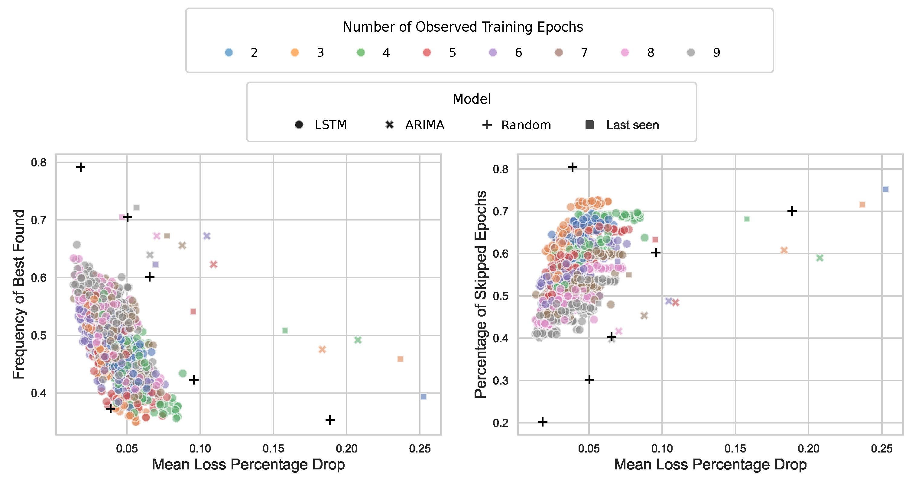
7.2. Results
The results of the simulation are presented in
Figure 11. Both performance estimators save approximately 42% to 65% of computation time (skipped epochs). However, an inverse trend is observed: as fewer epochs are observed, more epochs are discarded when a non-promising architecture is detected early, which slightly reduces the overall performance.
Additionally, we measure the frequency with which the estimator identifies the best solution, or ground truth. This likelihood increases as the number of observed epochs grows, suggesting that having more data leads to more accurate estimations.
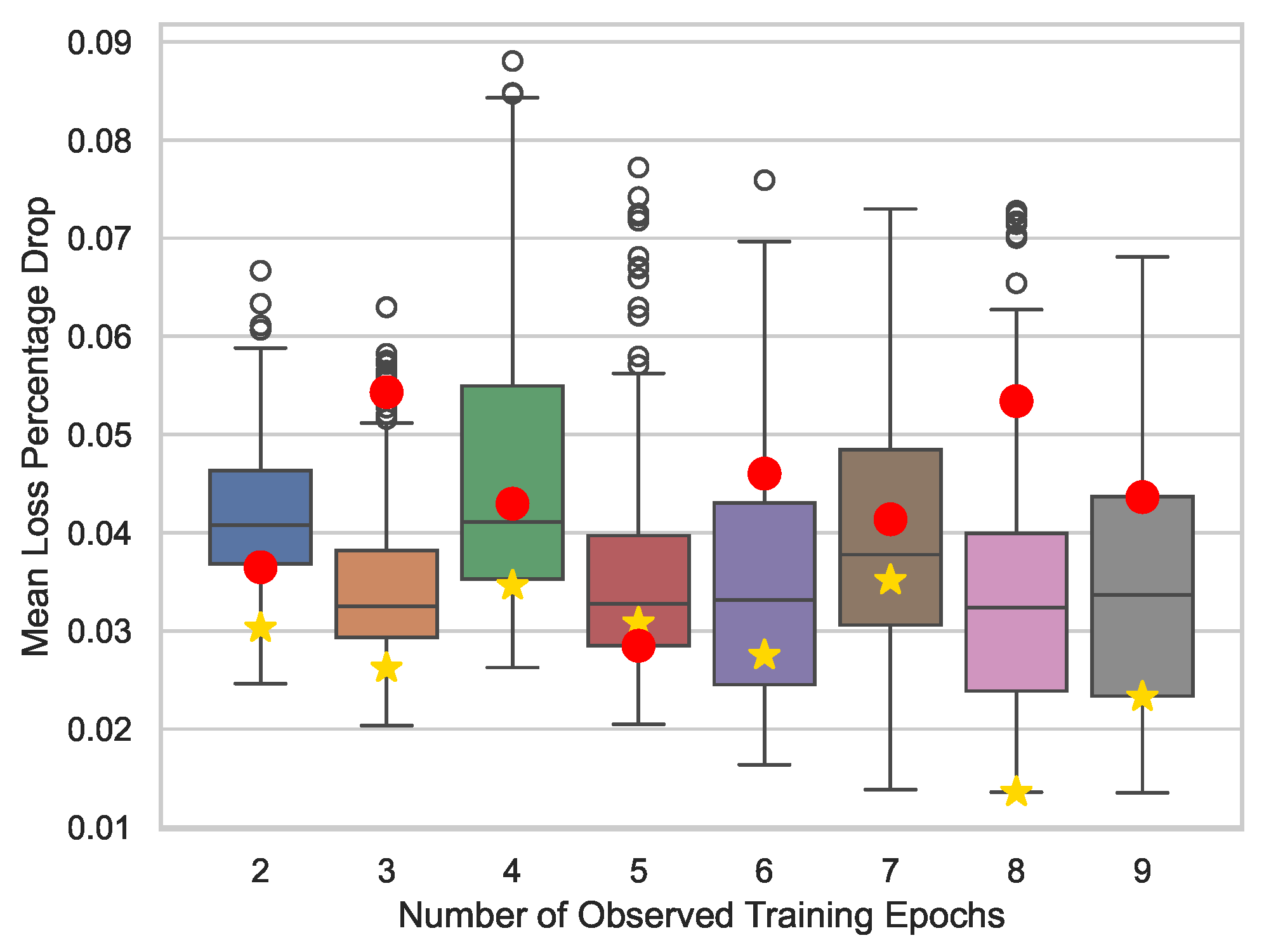
The effect of observing fewer epochs on the mean validation loss is also analyzed. On average, the increase in loss is minimal—approximately 2% in the worst-case scenario when only two epochs are observed (note that the learning curves are normalized between 0 and 1). This is evident from the star markers in
Figure 12. These results suggest that the negative impact of early stopping in BO, in terms of performance drop (
), is negligible, even when the number of observed epochs is limited. This finding aligns with the work of Egele et al. [
36], who demonstrated excellent performance even when observing only a single epoch.
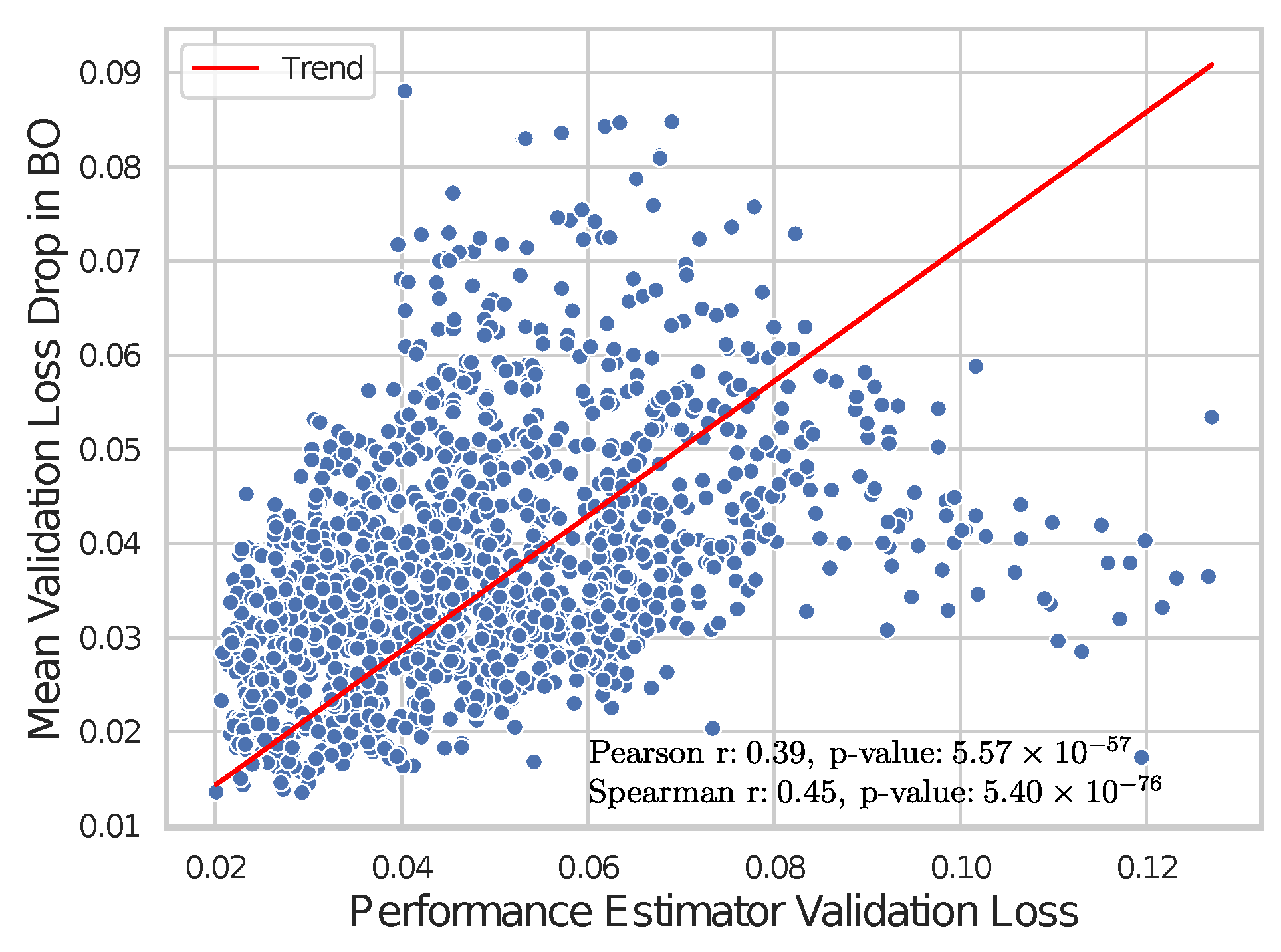
An important question, particularly regarding stability and reliability, is whether the predictive accuracy of the performance estimator translates effectively to the BO process. The star markers in
Figure 12 and
Figure 13 illustrate the correlation between the validation loss of the performance estimator and the mean increase in validation loss achieved during the BO process. The results indicate that a lower validation loss of the performance estimator corresponds to a lower increase in the mean validation loss during the BO process, highlighting the role of the estimator in guiding efficient model selection.
The observed moderate positive correlations (both Pearson and Spearman) indicate a relationship between the validation loss of the performance estimator and the BO efficiency of the process in identifying well-performing models, even when a significant percentage of epochs are discarded. Notably, the higher Spearman correlation compared to the Pearson correlation suggests that while the relationship may not be strictly linear, it follows a consistent monotonic trend. This insight highlights the importance of accurate performance estimation in enhancing the effectiveness of the BO process.
The inclusion of hyperparameters in the performance estimator results in just marginal improvements. While it enhances the prediction accuracy of the curve estimator, the benefits of incorporating network features become less pronounced if one looks at the BO process results. Conditioning aids in discarding poor-performing models, with only a minimal decrease in the mean loss percentage drop (see
Table 4), particularly when using only two observed epochs. This finding aligns with the greater variability in performance observed with fewer epochs, as illustrated in
Figure 9. Once both approaches converge, the amount of discarded training data becomes comparable, leading to similar average BO performance.
7.3. Performance Estimator Architecture Impact in the BO Process
Additionally, the potential impact of the hyperparameters of the estimator was analyzed. The hyperparameters studied included learning rate, network depth, bidirectionality, and recurrent units (width).
Figure 14 illustrates the effect of different ranges of values for each hyperparameter. Most hyperparameters appear to have no significant impact on the BO process, with the exception of the learning rate. For the non-conditioned estimator, higher learning rates are preferred, whereas for the conditioned estimator, this relationship is reversed.
7.4. Comparison with Baseline Models
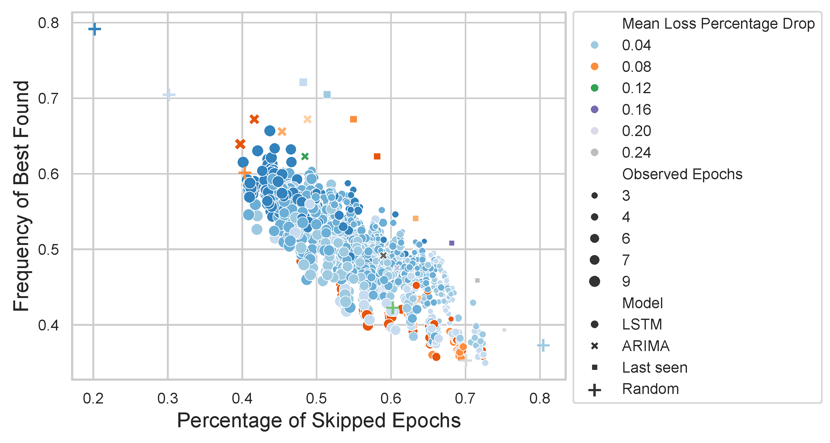
The proposed approach was evaluated against three baseline methods to assess its performance.
The first baseline is a random approach, where a percentage of training epochs is discarded at random. In
Figure 11 and
Figure 15, the results of the random baseline are represented with black plus symbols.
The second baseline leverages the “last seen value” as an approximation for the final performance. This approach is often competitive with more sophisticated learning curve extrapolation methods [
90]. Despite its simplicity, it has been effectively utilized in frameworks such as Hyperband [
32]. To ensure consistency in comparisons, the same early-stopping rule applied to our approach is also applied to this baseline. The results of the last-seen baseline are depicted in
Figure 11 and
Figure 15 using square markers.
The third baseline employs an ARIMA model to predict the final performance. The optimal parameters for the ARIMA algorithm—
p,
d, and
q—are determined based on the
T observed epochs. Using these parameters, the model forecasts up to 100 data points, representing the maximum number of epochs executed per model. As with the previous baselines, the same early-stopping rule applied to our approach is also applied here. The ARIMA baseline results are displayed in
Figure 11 and
Figure 15 using cross markers.
The results indicate that the random approach achieves competitive outcomes in terms of minimal performance drop, but only when a relatively small portion of training runs (20%) is discarded. In contrast, the proposed approach demonstrates superior performance, achieving better results while reducing the training time by 40%.
Similarly, the ARIMA baseline achieves a comparable 40% reduction in training time. However, this comes at the cost of a significant increase in the mean performance loss compared to the LSTM-based method.
Lastly, while the “last-seen value” baseline effectively minimizes training time and achieves impressive time savings, it exhibits a substantial increase in performance drop (). This underscores its limitations in maintaining performance consistency, particularly when compared to the proposed approach.
Test of Statistical Significance
To evaluate the statistical significance of the performance differences between the proposed approach and the baselines, a paired
t-test was conducted. The analysis compared the mean loss performance drop for different observed epochs. The
t-test statistic was calculated as
where
is the difference in mean performance drop between the proposed approach and the baseline,
s is the standard deviation of the paired differences, and
n is the number of paired observations. The resulting
p-value was computed as
where
represents the cumulative distribution function of the t-distribution. The results are displayed in
Table 5.
To ensure fairness, the comparison was limited to results within the range of epochs skipped by the ARIMA and "last-seen value" baselines. Against the ARIMA baseline, the test yielded a p-value of 0.007, demonstrating a statistically significant difference and confirming that the proposed method achieves a lower performance drop while avoiding a similar percentage of training epochs. Similarly, against the "last-seen value" baseline, a p-value of 0.0001 was obtained, indicating strong statistical significance.
For the random baseline, the p-value was 0.0002, highlighting a statistically significant improvement over the random approach. These results collectively confirm that the observed advantages of the proposed method are not due to random chance and underline its effectiveness compared to the baseline methods.
8. Theoretical Analysis
We do not wish to conclude the paper without addressing some key considerations about the two main elements of our proposal. Firstly, regarding the learning-curve estimator, it is important to discuss the potential impact of noise during the search for the optimal estimator. Secondly, with respect to Bayesian optimization (BO) for NAS, attention must be given to the implications of noise within the process.
It is assumed that, as is common when working with observational data, the noise satisfies
The likelihood of erroneous early stopping is influenced by several factors, including the noise variance (
), the selected tolerance factor
, and the characteristics of the noise process. To mitigate this risk, several strategies can be implemented. Increasing the tolerance factor
offers a safeguard against premature termination by allowing greater flexibility in the stopping criteria. Reducing the noise variance stabilizes the learning process, decreasing sensitivity to fluctuations. The influence on the convergence and suitability of BO under noise is an actively researched topic in the community (e.g., [
91]).
Due to space constraints, we focus on the current modeling approach, leaving the incorporation of additional dependencies, such as noise models of the form
for future research. For example, models such as
where
represents the architecture hyperparameters,
X denotes the dataset,
is the learning rate,
corresponds to the momentum, and
represents the stochastic noise process.
We now examine the question under two noise models.
8.1. On the Impact of Noise on Learning Curves on Early-Stopping Efficiency (I): Additive Noise
It is clear that noise in learning curves can affect the effectiveness of early stopping by complicating precise predictions of the future performance of the model. Robust pruning methods against noise could enhance BO efficiency in NAS.
In this section, we consider the decomposition of the learning curve as
where
represents the underlying (noise-free) learning curve, and
is a stochastic noise process, assumed to be autocorrelated. Recall that
.
The event of erroneous early stopping for a promising model can be defined as
where
T is the total number of training epochs, and
represents a tolerance factor. This indicates that the estimator
might prematurely discard a promising model.
Defining
, and noting that
, an upper bound for the probability of the event
E can be derived, namely,
Indeed,
Using the law of total variance,
In the case of the additive decomposition of the noise described earlier (and considering the independent variables), the event of erroneous early stopping,
and the noise could be approximated using the sum of the corresponding variances, with the noise decomposing as
8.2. On the Impact of Noise on Learning Curves on Early-Stopping Efficiency (II): Parametric (Autoregressive) Noise
To capture the complexity of learning curves with a more sophisticated model, the previous framework can be extended to account for advanced characteristics of the noise:
where
models a non-stationary noise model. In practice, the extended noise model follows an autoregressive law of the form
where
represents time-dependent autoregressive coefficients,
p is the order, and
represents noise conditional on the hyperparameters.
A reasonable hypothesis is that noise in the learning process can be effectively modeled using a first-order autoregressive process, capturing temporal dependencies that influence the variability throughout training:
where the temporal correlation is
. Considering the autoregressive structure, expectation and the effective variance would be
Thus, by the central limit theorem,
could be approximated by the normal distribution:
Under these conditions, the probability of erroneous early stopping is bounded by
The likelihood of erroneous early stopping depends on several factors, including the autocorrelation coefficient , the variance of the white noise , and the tolerance factor . As , the effective variance increases exponentially, indicating a stronger temporal dependency that amplifies the variability in the learning process. As , the behavior resembles white noise, where the temporal correlations decrease and the process approaches the characteristics of independent noise.
8.3. On the Convergence of Robust Early-Stopping Methods Under Noise
We discuss whether the pruning method is robust to noise, i.e., whether it converges somewhat to an estimate of the underlying learning curve with bounded error. This is an interesting aspect to study, as the noise present in the learning curves may affect the effectiveness of pruning during the BO process. Thus, we assume that the pruning method uses a filtering condition:
where
is a filtering function that decreases with
t.
Assume that the learning curve
is subject to random noise
:
where
is the underlying learning curve without noise.
Let
be an estimate of the learning curve
obtained using a noise-robust pruning method. We define the estimation error as
Then,
can be taken, such that
in probability; that is, the noise-robust pruning method converges to an estimate of the underlying learning curve with bounded error.
We begin by decomposing the error into two components:
Applying triangular inequality:
For the inequality of Chebyshev:
Therefore,
the second probability tends to 0 by the filtering condition. Thus,
Taking to be sufficiently large, is small, and we can assume that the error is bounded.
9. Discussion
This work proposes a methodology to improve the efficiency of NAS for PHM applications. A performance estimator capable of predicting the final validation performance of a model based on the initial training and validation performance curves has been developed. Two versions of the estimator were created: one using only the performance curves, and another that also incorporates the network hyperparameters. The estimators were trained and evaluated using a dataset of 61,000 learning curves generated from 62 different PHM datasets.
The results demonstrate that integrating the performance estimator into the BO process for NAS can significantly reduce the computational cost, achieving time savings of over 50%. There is a trade-off between the number of skipped epochs and the final performance of the BO process. The experiments show that the proposed approach achieves a performance drop between 3.5% and 1.5%, depending on the number of epochs observed, with an average drop of 2%. This drop is considered minimal in comparison to the time savings achieved.
In a certain sense, the approach discussed here aligns with the method proposed by Dai et al. [
34]. In their work, the authors employed a Bayesian model to predict when the model being trained during a BO iteration had sufficiently converged. This approach enabled earlier termination of training, thus avoiding unnecessary epochs. However, a limitation of this method is that it could still allow for training a model with little potential to outperform the current best model during a significant number of epochs. Such inefficiencies highlight the need for more refined stopping criteria, which may improve the trade-off between computational cost and model performance in BO-based optimization processes.
Our work goes a step further by training each model for a fixed, lower number N of epochs. During these N epochs, the learning curves are monitored and used by a previously trained network to estimate the final performance of the model. If the estimation indicates that the model performance is significantly worse than the best obtained so far, the training of the model is stopped. This approach aims to ensure that poorly performing models are trained for only N epochs.
This proposal could be valuable for the use of digital twins in studying PHM, a promising avenue (e.g., [
92]). Although the methodologies differ, both approaches aim to optimize decision making by anticipating the future behavior of a system. Digital twins, which rely on physical models to simulate real systems, could generate synthetic data to train and validate the neural models proposed in our approach, particularly in scenarios where real-world data are scarce. Conversely, machine learning techniques, such as those explored in this paper, could enhance the accuracy and efficiency of digital twins. This can be achieved by modeling complex system aspects that are difficult to capture with traditional physical models or by optimizing parameter selection within the digital twin framework. While this approach has been applied in the PHM domain to address a critical gap in the literature, the framework is inherently applicable across a wide range of fields.
Our study gains its insights through a simulated approach. Therefore, the next immediate work is to corroborate these findings with a real BO execution process.
Additionally, other points of improvement have been identified. In this work, the estimator is trained to make estimations with a fixed number N of observed epochs. In some cases, with a few more executions it becomes evident that a model will not perform well. Thus, estimating future performance at each epoch could help detect this and stop further executions.
An important aspect of our work is the emphasis on the diversity of datasets used during training and evaluation. While this diversity ensures that the proposed method is robust across a wide range of tasks and architectures, we did not explicitly analyze the performance differences of the trained neural networks across these datasets. Investigating such differences could reveal valuable insights into how dataset characteristics influence model performance and the effectiveness of our method. For instance, certain types of datasets may benefit more from learning curve predictions, while others might pose greater challenges. This unexplored dimension presents a promising avenue for future work, where a detailed analysis could help identify patterns and further improve the generalizability of our approach.
Regarding the hyperparameters used to condition the estimator, it could be interesting to include additional hyperparameters, such as meta-attributes about the dataset and the involved task. Studying how these meta-attributes could impact the estimator would be an interesting avenue for academic research.
Our method, while robust, has inherent limitations that must be acknowledged. In scenarios where the objective function does not guarantee convexity, our estimator may encounter significant challenges. These include the risk of converging to local minima, potential instability in performance estimation, and increased variability in predictions.
To address these challenges, we propose several mitigation mechanisms. First, we suggest using multiple random initializations to reduce the likelihood of becoming stuck in suboptimal solutions. Additionally, probabilistic restart techniques can be employed to explore different regions of the solution space, improving convergence. Finally, we recommend uncertainty estimation through bootstrapping to quantify the variability in the performance predictions and enhance the reliability of the estimates made by the model.
Our method may encounter certain other limitations under specific conditions. Firstly, the presence of significant noise in the data can decrease the accuracy of our predictions and increase the variability in the estimates. Noise interferes with the ability of the model to identify underlying patterns in the data, which results in less reliable predictions.
Secondly, when working with nonlinear architectures, our method may struggle to capture complex dynamics. This can lead to problems of overfitting or underfitting, as the model may not be able to adequately represent the relationships between the variables.
Finally, in domains with limited transferability, the generalization ability of the model may be compromised. The performance of our method can depend heavily on the specific characteristics of the domain, limiting its effectiveness when applied to different tasks or environments. These limitations will be the subject of future research.
Future work will focus on developing a more sophisticated state-space model for learning curves that captures the intricate dynamics of neural network training. For instance, this could involve modeling with an extended stochastic differential equation of the form
which incorporates architecture-dependent parameters through
, which captures layer complexity, connection types, and structural characteristics. Dataset dynamics are modeled by
, integrating dimensionality, entropy, and separability measures. Optimization processes are represented by
, explicitly accounting for learning rate, momentum, and adaptive optimization strategies. The noise process
is modeled as a correlated, time-dependent stochastic process, allowing for more nuanced capture of temporal dependencies and noise characteristics in learning dynamics.
Finally, it should be noted that the current method does not fully exploit the potential knowledge and adaptation capabilities of the performance curves generated during application to a new dataset. Incorporating few-shot learning to leverage these performance curves in ongoing experiments could be another area for improvement.
10. Conclusions
This study presents a methodology to enhance the efficiency of neural architecture search (NAS) in the PHM domain through the integration of a performance estimator. By leveraging the initial training and validation performance curves, the proposed estimator predicts the final validation performance of a model, offering a substantial reduction in computational cost. The experiments demonstrate that the approach achieves over 50% time savings with an average performance drop of just 2%, highlighting its minimal impact on model performance.
The proposed framework effectively addresses the trade-off between computational efficiency and final performance. Its robust design and adaptability make it applicable to a wide range of domains beyond PHM. While the current work provides significant insights, future research should explore further optimization of the estimator, incorporation of additional meta-attributes, and application to real-world scenarios to fully realize its potential. Overall, this methodology contributes to advancing resource-efficient NAS while maintaining high-quality model selection.


