Dynamics of an Impulsive Predator–Prey Model with a Seasonally Mass Migrating Prey Population

Abstract

Seasonality is a complex force in nature that affects multiple processes in wild animal populations. Animal mass migration refers to the migration of a large number of animals from a certain distance due to breeding, foraging, climate change or other reasons. In this work, an impulsive predator–prey model with a seasonally mass migrating prey population is constructed. The predator–extinction boundary periodic solution of system (3) is proved to be globally asymptotically stable. System (3) is also proved to be permanent. Our results provide a theoretical reference for biodiversity protection management.

1. Introduction

With the rapid loss of global biodiversity, the relationship between biodiversity and ecosystem stability has become an important scientific problem facing human beings [1]. Seasonality is a complex force in nature that affects multiple processes in wild animal populations. Animal mass migration refers to the migration of a large number of animals from a certain distance due to breeding, foraging, climate change or other reasons [2]. The migration of species is a common biological phenomenon which plays a major role in the stability of ecosystems. The effects of species migration between patches have received considerable attention in ecology. Migration has been described and studied in a variety of taxa from insects to higher vertebrates [3,4,5].

Mathematical ecology has its roots in population ecology, which examines the increase in and fluctuation of population [6]. Natural populations often exhibit some degree of spatial structure; that is, individuals interact more frequently with nearby than with distant organisms [7]. In most population models, diffusion between patches is assumed to be continuous or discrete [8,9]. The seasonal changes every year encourage the phenomenon of animal migration, which is often a seasonal and cyclical activity by which animals adapt to climate and food changes, or ensure successful reproduction. Animals migrate from their habitat to another area and return after a certain length of time [10]. The distribution of a species over its range of habitats is a fundamental and inseparable aspect of its interaction with its environment [11]. The effect of dispersal on population size and stability has been explored for a population that disperses passively between two discrete habitat patches. Robert [12] considered the following general model of density-dependent growth in two patches of equal size, linked symmetrically by passive dispersal:

$$\left\{\begin{array}{c}{\displaystyle \frac{d{N}_1}{dt}=N_1{\varphi }_1\left(N_1\right)-ϵN_1+ϵN_2,}\hfill \\ {\displaystyle \frac{d{N}_2}{dt}=N_2{\varphi }_2\left(N_2\right)+ϵN_1-ϵN_2,}\hfill \end{array}\right.$$

(1)

where $N_i(i=1,2)$ is the number of individuals in patch i, and the functions ${\varphi }_i$ encapsulate within-patch density-dependent processes influencing population growth. $ϵ>0$ is the dispersal rate. Recently, theories of impulsive differential equations have been introduced into population dynamics [13,14,15,16,17,18]. Especially, Wang et al. [19] investigated impulsive diffusion in a single-species model:

$$\left\{\begin{array}{c}\left.\begin{array}{c}{\displaystyle \frac{d{N}_1}{dt}=r_1{N}_{1}ln\frac{k_1}{N_1},}\hfill \\ {\displaystyle \frac{d{N}_2}{dt}=r_2{N}_{2}ln\frac{k_2}{N_2},}\hfill \end{array}\right\}t\ne n\tau ,\hfill \\ \left.\begin{array}{c}{\displaystyle △N_1=d(N_2-N_1),}\hfill \\ {\displaystyle △N_2=d(N_1-N_2),}\hfill \end{array}\right\}t=n\tau ,\hfill \end{array}\right.$$

(2)

where model (3) is constructed with two patches connected by diffusion, and $N_i$ is the density of species in the i-th patch. The intrinsic increasing rate of population in the i-th habitat is denoted by $r_i>0(i=1,2)$. $k_i>0(i=1,2)$ denotes the carrying capacity in the i-th patch, and $d_i>0(i=1,2))$ is dispersal rate in the i-th patch.

2. The Model

Motivated by the above discussion, we consider an impulsive predator–prey model with a seasonally mass migrating prey population

$$\left\{\begin{array}{c}\left.\begin{array}{c}{\displaystyle \frac{d{x}_1\left(t\right)}{dt}=x_1\left(t\right)(a_{11}-b_{11}{x}_1\left(t\right)),}\hfill \\ {\displaystyle \frac{d{x}_2\left(t\right)}{dt}=x_2\left(t\right)(a_{12}-b_{12}{x}_2\left(t\right)),}\hfill \\ {\displaystyle \frac{d{x}_3\left(t\right)}{dt}=x_3\left(t\right)(a_{13}-b_{13}{x}_3\left(t\right)),}\hfill \end{array}\right\}t\in (n\tau ,(n+l)\tau ],\hfill \\ \left.\begin{array}{c}{\displaystyle ▵x_1\left(t\right)=-{\epsilon }_1{x}_1\left(t\right),}\hfill \\ {\displaystyle ▵x_2\left(t\right)=0,}\hfill \\ {\displaystyle ▵x_3\left(t\right)=0,}\hfill \end{array}\right\}t=(n+l)\tau ,\hfill \\ \left.\begin{array}{c}{\displaystyle \frac{d{x}_1\left(t\right)}{dt}=x_1\left(t\right)(a_{21}-b_{21}{x}_1\left(t\right))-{\beta }_2{x}_1\left(t\right)x_2\left(t\right),}\hfill \\ {\displaystyle \frac{d{x}_2\left(t\right)}{dt}=x_2\left(t\right)(a_{22}-b_{22}{x}_2\left(t\right))+k_2{\beta }_2{x}_1\left(t\right)x_2\left(t\right),}\hfill \\ {\displaystyle \frac{d{x}_3\left(t\right)}{dt}=x_3\left(t\right)(a_{23}-b_{23}{x}_3\left(t\right)),}\hfill \end{array}\right\}t\in ((n+l)\tau ,(n+l+\eta )\tau ],\hfill \\ \left.\begin{array}{c}{\displaystyle ▵x_1\left(t\right)=-{\epsilon }_2{x}_1\left(t\right),}\hfill \\ {\displaystyle ▵x_2\left(t\right)=-h_2{x}_2\left(t\right),}\hfill \\ {\displaystyle ▵x_3\left(t\right)=0,}\hfill \end{array}\right\}t=(n+l+\eta )\tau ,\hfill \\ \left.\begin{array}{c}{\displaystyle \frac{d{x}_1\left(t\right)}{dt}=x_1\left(t\right)(a_{31}-b_{31}{x}_1\left(t\right))-{\beta }_3{x}_1\left(t\right)x_3\left(t\right),}\hfill \\ {\displaystyle \frac{d{x}_2\left(t\right)}{dt}=x_2\left(t\right)(a_{32}-b_{32}{x}_2\left(t\right)),}\hfill \\ {\displaystyle \frac{d{x}_3\left(t\right)}{dt}=x_3\left(t\right)(a_{33}-b_{33}{x}_3\left(t\right))+k_3{\beta }_3{x}_1\left(t\right)x_3\left(t\right),}\hfill \end{array}\right\}t\in ((n+l+\eta )\tau ,(n+1)\tau ],\hfill \\ \left.\begin{array}{c}{\displaystyle ▵x_1\left(t\right)=-{\epsilon }_3{x}_1\left(t\right),}\hfill \\ {\displaystyle ▵x_2\left(t\right)=0,}\hfill \\ {\displaystyle ▵x_3\left(t\right)=-h_3{x}_3\left(t\right),}\hfill \end{array}\right\}t=(n+1)\tau ,\hfill \end{array}\right.$$

(3)

where the prey population seasonally migrates between patch 1, patch 2 and patch $3.$ $x_1\left(t\right)$ is the density of the prey population at time $t.$ $x_2\left(t\right)$ is the density of predator population in patch 2 at time $t,$ and the predator population $x_2$ only lives in patch $2.$ $x_3\left(t\right)$ is the density of predator population in patch 3 at time $t,$ and predator population $x_3$ only lives in patch $3.$ $a_{11}>0$ is the intrinsic increasing rate of prey population $x_1$ in patch 1 on $(n\tau ,(n+l\left)\tau \right].$ $b_{11}>0$ is the intraspecific competition coefficient of prey population $x_1$ in patch 1 on $(n\tau ,(n+l\left)\tau \right].$ $a_{12}>0$ is the intrinsic increasing rate of predator population $x_2$ in patch 2 on $(n\tau ,(n+l\left)\tau \right].$ $b_{12}>0$ is the intraspecific competition coefficient of predator population $x_2$ in patch 2 on $(n\tau ,(n+l\left)\tau \right].$ $a_{13}>0$ is the intrinsic increasing rate of predator population $x_3$ in patch 3 on $(n\tau ,(n+l\left)\tau \right].$ $b_{13}>0$ is the intraspecific competition coefficient of predator population $x_3$ in patch 3 on $(n\tau ,(n+l\left)\tau \right].$ $0<{\epsilon }_1<1$ is the loss coefficient of the prey population during prey population $x_1$ mass migrating from patch 1 to patch 2 at $t=(n+l)\tau .$ $a_{21}>0$ is the intrinsic increasing rate of prey population $x_1$ in patch 2 on $\left(\right(n+l)\tau ,(n+l+\eta \left)\tau \right].$ $b_{21}>0$ is the intraspecific competition coefficient of prey population $x_1$ in patch 2 on $\left(\right(n+l)\tau ,(n+l+\eta \left)\tau \right].$ $a_{22}>0$ is the intrinsic increasing rate of predator population $x_2$ in patch 2 on $\left(\right(n+l)\tau ,(n+l+\eta \left)tau\right].$ $b_{22}>0$ is the intraspecific competition coefficient of predator population $x_2$ in patch 2 on $\left(\right(n+l)\tau ,(n+l+\eta \left)\tau \right].$ $a_{23}>0$ is the intrinsic increasing rate of predator population $x_3$ in patch 3 on $\left(\right(n+l+\eta )\tau ,(n+1\left)\right].$ $b_{23}>0$ is the intraspecific competition coefficient of predator population $x_3$ in patch 3 on $\left(\right(n+l)\tau ,(n+l+\eta \left)\tau \right].$ ${\beta }_2>0$ is the catchable coefficient of the prey population by predator population $x_2$ in patch 2 on $\left(\right(n+l+\eta )\tau ,(n+1\left)\tau \right]$. $k_2>0$ is the rate of conversion of nutrients into the reproduction rate of the predator population $x_2$ in patch 2 on $\left(\right(n+l+\eta )\tau ,(n+1\left)\tau \right].$ $0<{\epsilon }_2<1$ is the loss coefficient of prey population $x_1$ mass migrating from patch 2 to patch 3 at $t=(n+l+\eta )\tau .$ $0<h_2<1$ is the harvesting coefficient of predator population $x_2$ while the mass prey population $x_1$ migrates from patch 2 to patch 3 at $t=(n+l+\eta )\tau .$ $a_{31}>0$ is the intrinsic increasing rate of prey population $x_1$ in patch 3 on $\left(\right(n+l+\eta )\tau ,(n+1\left)\tau \right].$ $b_{31}>0$ is the intraspecific competition coefficient of prey population $x_1$ in patch 3 on $\left(\right(n+l+\eta )\tau ,(n+1\left)\tau \right].$ $a_{32}>0$ is the intrinsic increasing rate of predator population $x_2$ in patch 2 on $\left(\right(n+l+\eta )\tau ,(n+1\left)\tau \right].$ $b_{32}>0$ is the intraspecific competition coefficient of predator population $x_2$ in patch 2 on $\left(\right(n+l+\eta )\tau ,(n+1\left)\tau \right].$ $a_{33}>0$ is the intrinsic increasing rate of predator population $x_3$ in patch 3 on $\left(\right(n+l)\tau ,(n+1+\eta \left)\tau \right].$ $b_{33}>0$ is the intraspecific competition coefficient of the predator population $x_3$ in patch 3 on $\left(\right(n+l+\eta )\tau ,(n+1\left)\tau \right].$ ${\beta }_3>0$ is the catchable coefficient of the prey population by predator population $x_3$ in patch 3 on $\left(\right(n+l+\eta )\tau ,(n+1\left)\tau \right]$. $k_3>0$ is the rate of conversion of nutrients into the reproduction rate of the predator population $x_3$ in patch 3 on $\left(\right(n+l+\eta )\tau ,(n+1\left)\tau \right].$ $0<{\epsilon }_3<1$ is the loss coefficient of prey population $x_1$ mass migrating from patch 3 to patch 1 at $t=(n+1)\tau .$ $0<h_2<1$ is the harvesting coefficient of predator population $x_3$ while prey population $x_1$ mass migrates from patch 3 to patch 1 at $t=(n+1)\tau .$ The mass migration of the prey population occurs every $\tau$ period ($\tau$ is a positive constant; $0<l<1$, and $0<l+\eta <1$), and $▵x_i\left(t\right)=x_i\left(t^{+}\right)-x_i\left(t\right)(i=1,2,3).$

3. Lemmas and Definition

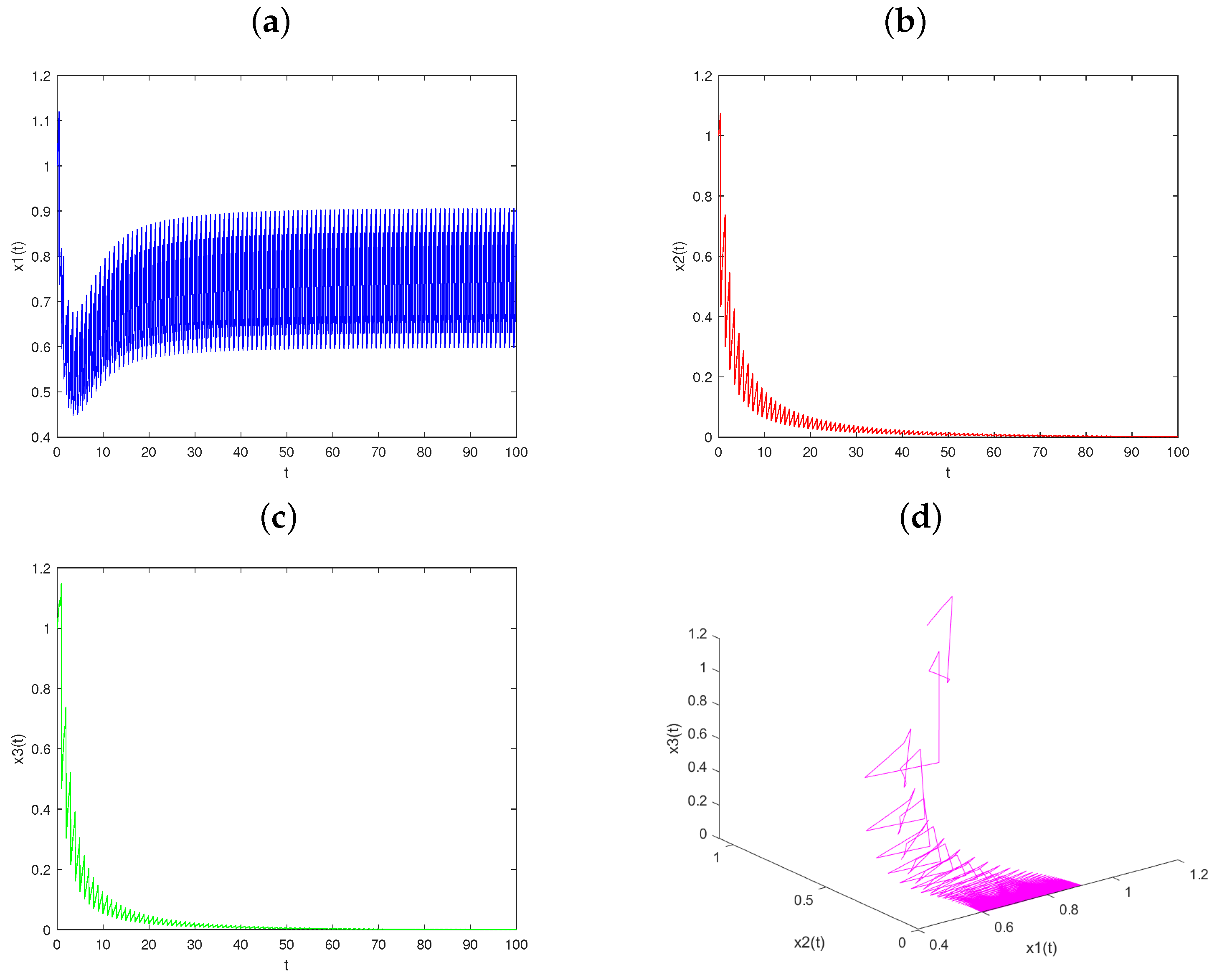
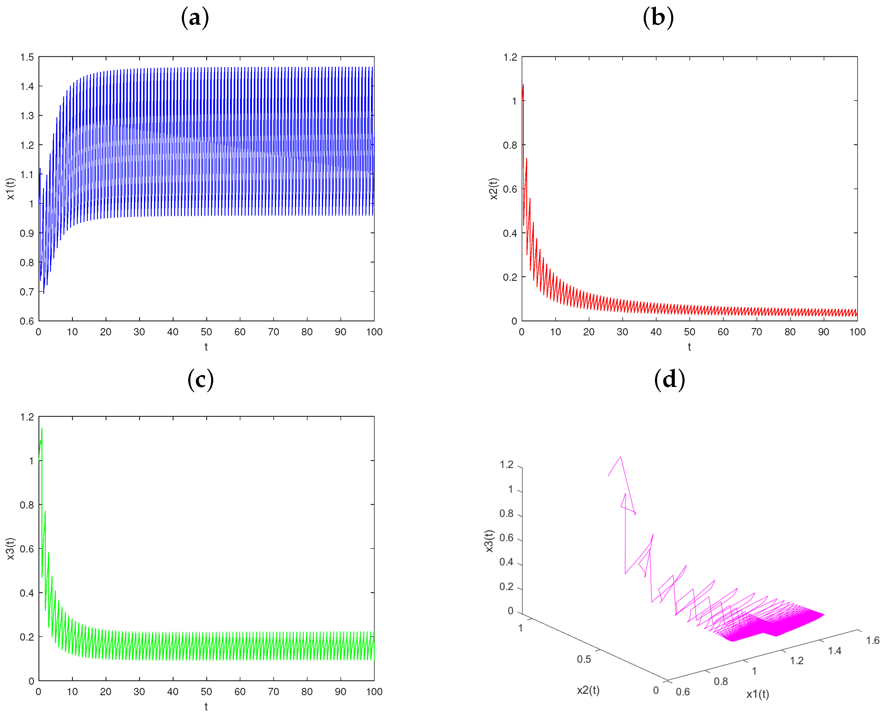
Let $f=(f_1,f_2,f_3)$, and let the map defined by the right side of system (3). The solution of system (3), denoted by $X\left(t\right)={(x_1\left(t\right),x_2\left(t\right),x_3\left(t\right))}^T$, is a piecewise continuous function X: $R_{+}\to R_{+}^3$, where $R_{+}=[0,\infty ),R_{+}^3=\{X\in R^3:X>0\}$. $X\left(t\right)$ is continuous on $(n\tau ,(n+l)\tau ]\times R_{+}^3$, $((n+l)\tau ,(n+l+\eta )\tau ]\times R_{+}^3(n\in Z_{+}$ and $((n+l+\eta )\tau ,(n+1)\tau ]\times R_{+}^3(n\in Z_{+})$. According to reference [16], the global existence and uniqueness of solutions of system (3) is guaranteed by the smoothness properties of f, which denote the mapping defined by right side of system (3).

Lemma 1. 

There exists a constant $M>0$ such that $x_i\left(t\right)\le M(i=1,2,3)$ with sufficient t in system (3).

Proof. 

Defining $V\left(t\right)=k_1{x}_1\left(t\right)+x_2\left(t\right)+x_3\left(t\right)$ with $k_1=max\{k_2,k_3\},$ we can obtain the following differential inequality for $t\in (n\tau ,(n+l\left)\tau \right]$

$$D^{+}V\left(t\right)+V\left(t\right)$$

$$<-k_1{b}_{11}{(x_1\left(t\right)-{\displaystyle \frac{a_{11}+1}{2b_{11}}})}^2+{\displaystyle \frac{k_1{(a_{11}+1)}^2}{4b_{11}}}-b_{12}{(x_2\left(t\right)-{\displaystyle \frac{a_{12}+1}{2b_{12}}})}^2$$

$$+{\displaystyle \frac{{(a_{12}+1)}^2}{4b_{12}}}-b_{13}{(x_3\left(t\right)-{\displaystyle \frac{a_{13}+1}{2b_{13}}})}^2+{\displaystyle \frac{{(a_{13}+1)}^2}{4b_{13}}}$$

$$\le {\displaystyle \frac{k_1{(a_{11}+1)}^2}{4b_{11}}}+{\displaystyle \frac{{(a_{12}+1)}^2}{4b_{12}}}+{\displaystyle \frac{{(a_{13}+1)}^2}{4b_{13}}}\stackrel{\Delta }{=}{M}_1.$$

For $t\in \left(\right(n+l)\tau ,(n+1+\eta \left)\tau \right]$, the following is easily obtained

$$D^{+}V\left(t\right)+V\left(t\right)$$

$$=-k_1{b}_{21}{(x_1\left(t\right)-{\displaystyle \frac{a_{21}+1}{2b_{21}}})}^2+{\displaystyle \frac{k_1{(a_{21}+1)}^2}{4b_{21}}}-b_{22}{(x_2\left(t\right)-{\displaystyle \frac{a_{22}+1}{2b_{22}}})}^2$$

$$+{\displaystyle \frac{{(a_{22}+1)}^2}{4b_{22}}}-b_{23}{(x_3\left(t\right)-{\displaystyle \frac{a_{23}+1}{2b_{23}}})}^2+{\displaystyle \frac{{(a_{23}+1)}^2}{4b_{23}}}$$

$$\le {\displaystyle \frac{k_1{(a_{21}+1)}^2}{4b_{21}}}+{\displaystyle \frac{{(a_{22}+1)}^2}{4b_{22}}}+{\displaystyle \frac{{(a_{23}+1)}^2}{4b_{23}}}\stackrel{\Delta }{=}{M}_2,$$

For $t\in \left(\right(n+l+\eta )\tau ,(n+1\left)\tau \right]$, the following is easily obtained

$$D^{+}V\left(t\right)+V\left(t\right)$$

$$=-k_1{b}_{31}{(x_1\left(t\right)-{\displaystyle \frac{a_{31}+1}{2b_{31}}})}^2+{\displaystyle \frac{k_1{(a_{31}+1)}^2}{4b_{31}}}-b_{32}{(x_2\left(t\right)-{\displaystyle \frac{a_{32}+1}{2b_{32}}})}^2$$

$$+{\displaystyle \frac{{(a_{32}+1)}^2}{4b_{32}}}-b_{33}{(x_3\left(t\right)-{\displaystyle \frac{a_{33}+1}{2b_{33}}})}^2+{\displaystyle \frac{{(a_{33}+1)}^2}{4b_{33}}}$$

$$\le {\displaystyle \frac{k_1{(a_{31}+1)}^2}{4b_{31}}}+{\displaystyle \frac{{(a_{32}+1)}^2}{4b_{32}}}+{\displaystyle \frac{{(a_{33}+1)}^2}{4b_{33}}}\stackrel{\Delta }{=}{M}_3.$$

Then, taking $M_0=max\{M_1,M_2,M_3\},$ when $t\ne n\tau ,t\ne (n+l+\eta )\tau$ and $t\ne (n+1)\tau ,$ we have

$$D^{+}V\left(t\right)+V\left(t\right)\le M_0.$$

For $t=(n+l)\tau ,$ we have $V\left((n+l){\tau }^{+}\right)\le k_1(1-{\epsilon }_1)x_1\left((n+l)\tau \right)+x_2\left((n+l)\tau \right)+x_3\left((n+l)\tau \right)\le V\left((n+l)\tau \right)$. For $t=(n+l+\eta )\tau ,$ we have $V\left((n+l+\eta ){\tau }^{+}\right)\le k_1(1-{\epsilon }_2)x_1\left((n+l)\tau \right)+(1-h_1)x_2\left((n+l+\eta )\tau \right)+x_3\left((n+l+\eta )\tau \right)\le V\left((n+l+\eta )\tau \right)$. For $t=(n+1)\tau ,$ we have $V\left((n+1){\tau }^{+}\right)=k_1(1-{\epsilon }_3)x_1\left((n+1)\tau \right)+x_2\left((n+1)\tau \right)+(1-h_2)x_3\left((n+1)\tau \right)\le V\left((n+1)\tau \right)$. According to the lemma of reference [16], for $t\in (n\tau ,(n+l\left)\tau \right]$, $t\in \left(\right(n+l)\tau ,(n+l+\eta \left)\tau \right],$ and $t\in \left(\right(n+l+\eta )\tau ,(n+1\left)\tau \right],$ we have

$$V\left(t\right)\le V\left(0\right)exp(-t)+{\int }_0^t{M}_{0}exp(-(t-s))ds$$

$$<V\left(0\right)exp(-t)+M_0(1-exp(-t))$$

$$\to M_0,ast\to \infty .$$

So, $V\left(t\right)$ is uniformly ultimately bounded. According to the definition of $V\left(t\right)$, there exists a constant $M>0$ such that $x_i\left(t\right)\le M(i=1,2,3)$ for sufficient t. □

Lemma 2. 

([17]). Considering the following difference equation

$$\begin{array}{c}{\displaystyle x\left(\right(t+1\left)\right)=F\left(x\right(t\left)\right),}\hfill \end{array}$$

(4)

$x^{*}$ satisfies

$$\begin{array}{c}{\displaystyle x^{*}=F\left(x^{*}\right),}\hfill \end{array}$$

(5)

then $x^{*}$ is called a equilibrium of (4), and if

$$\begin{array}{c}{\displaystyle \frac{\partial F\left(x\right)}{\partial x}{|}_{x=x^{*}}<1,}\hfill \end{array}$$

(6)

then, the unique equilibrium $x^{*}$ of difference Equation (5) is globally asymptotically stable. Otherwise, it is not stable.

If $x_i\left(t\right)=0(i=2,3),$ one subsystem of system (3) can be obtained as

$$\left\{\begin{array}{c}\begin{array}{c}{\displaystyle \frac{d{x}_1\left(t\right)}{dt}=x_1\left(t\right)(a_{11}-b_{11}{x}_1\left(t\right)),t\in (n\tau ,(n+l)\tau ],}\hfill \end{array}\hfill \\ \begin{array}{c}{\displaystyle ▵x_1\left(t\right)=-{\epsilon }_1{x}_1\left(t\right),t=(n+l)\tau ,}\hfill \end{array}\hfill \\ \begin{array}{c}{\displaystyle \frac{d{x}_1\left(t\right)}{dt}=x_1\left(t\right)(a_{21}-b_{21}{x}_1\left(t\right)),t\in ((n+l+\eta )\tau ,(n+l+\eta )\tau ],}\hfill \end{array}\hfill \\ \begin{array}{c}{\displaystyle ▵x_1\left(t\right)=-{\epsilon }_2{x}_1\left(t\right),t=(n+l+\eta )\tau .}\hfill \end{array}\hfill \\ \begin{array}{c}{\displaystyle \frac{d{x}_1\left(t\right)}{dt}=x_1\left(t\right)(a_{31}-b_{31}{x}_1\left(t\right)),t\in ((n+l+\eta )\tau ,(n+1)\tau ],}\hfill \end{array}\hfill \\ \begin{array}{c}{\displaystyle ▵x_1\left(t\right)=-{\epsilon }_3{x}_1\left(t\right),t=(n+1)\tau .}\hfill \end{array}\hfill \end{array}\right.$$

(7)

The analytic solution of system (7) between pulses is obtained as

$$\begin{array}{c}\begin{array}{c}{\displaystyle x_1\left(t\right)=}\hfill \end{array}\left\{\begin{array}{c}{\displaystyle \frac{x_1\left(n{\tau }^{+}\right)e^{a_{11}(t-n\tau )}}{a_{11}+b_{11}{x}_1\left(n\tau \right)(e^{a_{11}(t-n\tau )}-1)},t\in (n\tau ,(n+l)\tau ],}\hfill \\ {\displaystyle \frac{x_1\left((n+l){\tau }^{+}\right)e^{a_{21}(t-(n+l)\tau )}}{a_{21}+b_{21}{x}_1\left((n+l)\tau \right)(e^{a_{21}(t-(n+l)\tau )}-1)},}\hfill \\ {\displaystyle t\in \left(\right(n+l)\tau ,(n+l+\eta \left)\tau \right].}\hfill \\ {\displaystyle \frac{x_1\left((n+l+\eta ){\tau }^{+}\right)e^{a_{31}(t-(n+l+\eta )\tau )}}{a_{31}+b_{31}{x}_1\left((n+l+\eta )\tau \right)(e^{a_{31}(t-(n+l+\eta )\tau )}-1)},}\hfill \\ {\displaystyle t\in \left(\right(n+l+\eta )\tau ,(n+1\left)\tau \right].}\hfill \end{array}\right.\hfill \end{array}$$

(8)

We compute the stroboscopic map of system (7)

$$\begin{array}{c}{\displaystyle x_1\left((n+1){\tau }^{+}\right)}\hfill \\ {\displaystyle =\frac{A_{11}{A}_{21}{A}_{31}{x}_1\left(n{\tau }^{+}\right)}{a_{11}{a}_{21}{a}_{31}+(B_{11}{a}_{21}{a}_{31}+A_{11}{B}_{21}{a}_{31}+A_{11}{A}_{21}{B}_{31})x_1\left(n{\tau }^{+}\right)}.}\hfill \end{array}$$

(9)

with $A_{11}=(1-{\epsilon }_1)e^{a_{11}l\tau },B_{11}=b_{11}(e^{a_{11}l\tau }-1),$$A_{21}=(1-{\epsilon }_2)e^{a_{21}\eta \tau },B_{21}=b_{21}(e^{a_{21}\eta \tau }-1),$$A_{31}=(1-{\epsilon }_3)e^{a_{31}(1-l-\eta )\tau },B_{31}=b_{31}(e^{a_{31}(1-l-\eta )\tau }-1).$ Two fixed points of (9) are obtained as $x_1^0=0$ and

$$\begin{array}{c}{\displaystyle x_1^{*}=\frac{A_{11}{A}_{21}{A}_{31}-a_{11}{a}_{21}{a}_{31}}{B_{11}{a}_{21}{a}_{31}+A_{11}{B}_{21}{a}_{31}+A_{11}{A}_{21}{B}_{31}},A_{11}{A}_{21}{A}_{31}>a_{11}{a}_{21}{a}_{31}.}\hfill \end{array}$$

(10)

Lemma 3. 

(i) If $A_{11}{A}_{21}{A}_{31}<a_{11}{a}_{21}{a}_{31},$ the fixed point $x_1^0$ of (9) is globally asymptotically stable.

(ii) If $A_{11}{A}_{21}{A}_{31}>a_{11}{a}_{21}{a}_{31},$ the fixed point $x_1^{*},$ of (9) is globally asymptotically stable; here, $x_1^{*}$ is defined as (10).

Proof. 

Using the following notation

$$\begin{array}{c}{\displaystyle F\left(x_1\left(n{\tau }^{+}\right)\right)=\frac{A_{11}{A}_{21}{A}_{31}{x}_1\left(n{\tau }^{+}\right)}{a_{11}{a}_{21}{a}_{31}+(B_{11}{a}_{21}{a}_{31}+A_{11}{B}_{21}{a}_{31}+A_{11}{A}_{21}{B}_{31})x_1\left(n{\tau }^{+}\right)},}\hfill \end{array}$$

(11)

we change (11) to

$$\begin{array}{c}{\displaystyle x_1\left((n+1){\tau }^{+}\right)=F\left(x_1\left(n{\tau }^{+}\right)\right)}\hfill \\ {\displaystyle =\frac{A_{11}{A}_{21}{A}_{31}{x}_1\left(n{\tau }^{+}\right)}{a_{11}{a}_{21}{a}_{31}+(B_{11}{a}_{21}{a}_{31}+A_{11}{B}_{21}{a}_{31}+A_{11}{A}_{21}{B}_{31})x_1\left(n{\tau }^{+}\right)},}\hfill \end{array}$$

(12)

then,

$$\begin{array}{c}{\displaystyle \frac{\partial F\left(x_1\left(n{\tau }^{+}\right)\right)}{\partial x_1\left(n{\tau }^{+}\right)}}\hfill \\ {\displaystyle =\frac{A_{11}{A}_{21}{A}_{31}{a}_{11}{a}_{21}{a}_{31}}{{[a_{11}{a}_{21}{a}_{31}+(B_{11}{a}_{21}{a}_{31}+A_{11}{B}_{21}{a}_{31}+A_{11}{A}_{21}{B}_{31})x_1\left(n{\tau }^{+}\right)]}^2}.}\hfill \end{array}$$

(13)

$\left(i\right)$ If $A_{11}{A}_{21}{A}_{31}<a_{11}{a}_{21}{a}_{31},$$x_1^0$ is a unique fixed point of (9), then we have

$$\begin{array}{c}{\displaystyle \frac{\partial F\left(x_1\left(n{\tau }^{+}\right)\right)}{\partial x_1\left(n{\tau }^{+}\right)}{|}_{x_1\left(n{\tau }^{+}\right)=0}}\hfill \\ {\displaystyle =\frac{A_{11}{A}_{21}{A}_{31}{a}_{11}{a}_{21}{a}_{31}}{{[a_{11}{a}_{21}{a}_{31}+(B_{11}{a}_{21}{a}_{31}+A_{11}{B}_{21}{a}_{31}+A_{11}{A}_{21}{B}_{31})x_1\left(n{\tau }^{+}\right)]}^2}{|}_{x_1\left(n{\tau }^{+}\right)=0}}\hfill \\ {\displaystyle =\frac{A_{11}{A}_{21}{A}_{31}}{a_{11}{a}_{21}{a}_{13}}<1.}\hfill \end{array}$$

(14)

From Lemma 2, we obtain that fixed point $x_1^0$ of (9) is globally asymptotically stable.

$\left(ii\right)$ If $A_{11}{A}_{21}{A}_{31}>a_{11}{a}_{21}{a}_{31},$$x_1^{*}$ is one fixed point of (9), then we have

$$\begin{array}{c}{\displaystyle \frac{\partial F\left(x_1\left(n{\tau }^{+}\right)\right)}{\partial x_1\left(n{\tau }^{+}\right)}{|}_{x_1\left(n{\tau }^{+}\right)=0}}\hfill \\ {\displaystyle =\frac{A_{11}{A}_{21}{A}_{31}{a}_{11}{a}_{21}{a}_{31}}{{[a_{11}{a}_{21}{a}_{31}+(B_{11}{a}_{21}{a}_{31}+A_{11}{B}_{21}{a}_{31}+A_{11}{A}_{21}{B}_{31})x_1\left(n{\tau }^{+}\right)]}^2}{|}_{x_1\left(n{\tau }^{+}\right)=0}}\hfill \\ {\displaystyle =\frac{A_{11}{A}_{21}{A}_{31}}{a_{11}{a}_{21}{a}_{31}}>1.}\hfill \end{array}$$

(15)

Then, we obtain that fixed point $x_1^0$ of (9) is unstable. $x_1^{*}$ is another fixed point of $\left(9\right)$, then we have

$$\begin{array}{c}{\displaystyle \frac{\partial F\left(x_1\left(n{\tau }^{+}\right)\right)}{\partial x_1\left(n{\tau }^{+}\right)}{|}_{x_1\left(n{\tau }^{+}\right)=x_1^{*}}}\hfill \\ {\displaystyle =\frac{A_{11}{A}_{21}{A}_{31}{a}_{11}{a}_{21}{a}_{31}}{{[a_{11}{a}_{21}{a}_{31}+(B_{11}{a}_{21}{a}_{31}+A_{11}{B}_{21}{a}_{31}+A_{11}{A}_{21}{B}_{31})x_1\left(n{\tau }^{+}\right)]}^2}{|}_{x_1\left(n{\tau }^{+}\right)=x_1^{*}}}\hfill \\ {\displaystyle =\frac{a_{11}{a}_{21}{a}_{31}}{A_{11}{A}_{21}{A}_{31}}<1.}\hfill \end{array}$$

(16)

From Lemma 2, we obtain that fixed point $x^{*}$ of (10) is locally stable. Furthermore, it is globally asymptotically stable.

Similar to [18], we can easily obtain the following lemma. □

Lemma 4. 

$\left(i\right)$ If $A_{11}{A}_{21}{A}_{31}<a_{11}{a}_{21}{a}_{31},$ the trivial periodic solutions of system (7) is globally asymptotically stable.

$\left(ii\right)$ If $A_{11}{A}_{21}{A}_{31}>a_{11}{a}_{21}{a}_{31},$ the periodic solution $\widetilde{x_1\left(t\right)}$ of system (7) is globally asymptotically stable, where $\widetilde{x_1\left(t\right)}$ is defined as

$$\begin{array}{c}\begin{array}{c}{\displaystyle \widetilde{x_1\left(t\right)}=}\hfill \end{array}\left\{\begin{array}{c}{\displaystyle \frac{x_1^{*}{e}^{a_{11}(t-n\tau )}}{a_{11}+b_{11}{x}_1^{*}(e^{a_{11}(t-n\tau )}-1)},t\in (n\tau ,(n+l)\tau ],}\hfill \\ {\displaystyle \frac{x_1^{**}{e}^{a_{21}(t-(n+l)\tau )}}{a_{21}+b_{21}{x}_1^{**}(e^{a_{21}(t-(n+l)\tau )}-1)},t\in ((n+l)\tau ,(n+l+\eta )\tau ],}\hfill \\ {\displaystyle \frac{x_1^{***}{e}^{a_{31}(t-(n+l+\eta )\tau )}}{a_{31}+b_{31}{x}_1^{***}(e^{a_{31}(t-(n+l+\eta )\tau )}-1)},t\in ((n+l+\eta )\tau ,(n+1)\tau ],}\hfill \end{array}\right.\hfill \end{array}$$

(17)

where $x_1^{*}$ is defined as (10) and

$$\begin{array}{c}{\displaystyle x_1^{**}=\frac{x_1^{*}(1-{\epsilon }_1)e^{a_{11}l\tau }}{a_{11}+b_{11}{x}_1^{*}(e^{a_{11}l\tau }-1)},x_1^{***}=\frac{x_1^{**}(1-{\epsilon }_2)e^{a_{21}\eta \tau }}{a_{21}+b_{21}{x}_1^{**}(e^{a_{21}\eta \tau }-1)}.}\hfill \end{array}$$

(18)

If $x_1\left(t\right)=0,$ the other two subsystems of system (3) are

$$\left\{\begin{array}{c}{\displaystyle \frac{d{x}_2\left(t\right)}{dt}=x_2\left(t\right)(a_{12}-b_{12}{x}_2\left(t\right)),t\in (n\tau ,(n+l)\tau ],}\hfill \\ {\displaystyle ▵x_2\left(t\right)=0,t=(n+l)\tau ,}\hfill \\ {\displaystyle \frac{d{x}_2\left(t\right)}{dt}=x_2\left(t\right)(a_{22}-b_{22}{x}_2\left(t\right)),t=((n+l)\tau ,(n+l+\eta )\tau ],}\hfill \\ {\displaystyle ▵x_2\left(t\right)=-h_2{x}_2\left(t\right),t=(n+l+\eta )\tau ,}\hfill \\ {\displaystyle \frac{d{x}_2\left(t\right)}{dt}=x_2\left(t\right)(a_{32}-b_{32}{x}_2\left(t\right)),t=((n+l+\eta )\tau ,(n+1)\tau ],}\hfill \\ {\displaystyle ▵x_2\left(t\right)=0,t=(n+1)\tau ,}\hfill \end{array}\right.$$

(19)

and

$$\left\{\begin{array}{c}{\displaystyle \frac{d{x}_3\left(t\right)}{dt}=x_3\left(t\right)(a_{13}-b_{13}{x}_3\left(t\right)),t\in (n\tau ,(n+l)\tau ],}\hfill \\ {\displaystyle ▵x_3\left(t\right)=0,t=(n+l)\tau ,}\hfill \\ {\displaystyle \frac{d{x}_3\left(t\right)}{dt}=x_3\left(t\right)(a_{23}-b_{23}{x}_3\left(t\right)),t=((n+l)\tau ,(n+l+\eta )\tau ],}\hfill \\ {\displaystyle ▵x_3\left(t\right)=0,t=(n+l+\eta )\tau ,}\hfill \\ {\displaystyle \frac{d{x}_3\left(t\right)}{dt}=x_3\left(t\right)(a_{32}-b_{33}{x}_3\left(t\right)),t=((n+l+\eta )\tau ,(n+1)\tau ],}\hfill \\ {\displaystyle ▵x_3\left(t\right)=-h_3{x}_3\left(t\right),t=(n+1)\tau .}\hfill \end{array}\right.$$

(20)

The stroboscopic maps of system (19) and (20) are

$$\begin{array}{c}{\displaystyle x_2\left((n+1){\tau }^{+}\right)=\frac{A_1{x}_2\left(n{\tau }^{+}\right)}{a_{12}{a}_{22}{a}_{32}+B_1{x}_2\left(n{\tau }^{+}\right)},}\hfill \end{array}$$

(21)

and

$$\begin{array}{c}{\displaystyle x_3\left((n+1){\tau }^{+}\right)=\frac{A_2{x}_3\left(n{\tau }^{+}\right)}{a_{13}{a}_{23}{a}_{33}+B_2{x}_3\left(n{\tau }^{+}\right)},}\hfill \end{array}$$

(22)

with $A_1=(1-h_2)e^{[a_{12}l+a_{22}\eta +a_{32}(1-l-\eta )]\tau },$$B_1=b_{12}{a}_{22}{a}_{32}(e^{a_{12}l\tau }-1)+b_{22}{a}_{32}{e}^{a_{12}l\tau }(e^{a_{22}\eta }-1)+(1-h_2)b_{32}{e}^{(a_{12}l+a_{32}\eta )\tau }(e^{a_{32}(1-l-\eta )\tau }-1),$ $A_2=(1-h_3)e^{[a_{13}l+a_{23}\eta +a_{33}(1-l-\eta )]\tau },$$B_2=b_{13}{a}_{23}{a}_{33}(e^{a_{13}l\tau }-1)+b_{23}{a}_{33}{e}^{a_{13}l\tau }(e^{a_{23}\eta }-1)+(1-h_3)b_{33}{e}^{(a_{13}l+a_{33}\eta )\tau }(e^{a_{33}(1-l-\eta )\tau }-1).$

Similar to Lemmas 3 and 4, we can obtain

Lemma 5. 

$\left(i\right)$ If $(1-h_2)e^{[a_{12}l+a_{22}\eta +a_{32}(1-l-\eta )]\tau }<a_{12}{a}_{22}{a}_{32},$ the fixed point $x_2^0$ of (21) is globally asymptotically stable.

$\left(ii\right)$ If $(1-h_3)e^{[a_{13}l+a_{23}\eta +a_{33}(1-l-\eta )]\tau }<a_{13}{a}_{23}{a}_{33},$ the fixed point $x_3^0$ of (22) is globally asymptotically stable.

$\left(iii\right)$ If $(1-h_2)e^{[a_{12}l+a_{22}\eta +a_{32}(1-l-\eta )]\tau }>a_{12}{a}_{22}{a}_{32},$ the fixed point $x_2^{*}$ of (21) is globally asymptotically stable.

$\left(iv\right)$ If $(1-h_3)e^{[a_{13}l+a_{23}\eta +a_{33}(1-l-\eta )]\tau }>a_{13}{a}_{23}{a}_{33},$ the fixed point $x_3^{*}$ of (22) is globally asymptotically stable. $x_2^{*}$ and $x_3^{*}$ are

$$\begin{array}{c}{\displaystyle x_2^{*}=\frac{A_1-a_{12}{a}_{22}{a}_{32}}{B_1},}\hfill \end{array}$$

(23)

and

$$\begin{array}{c}{\displaystyle x_3^{*}=\frac{A_2-a_{13}{a}_{23}{a}_{33}}{B_2}.}\hfill \end{array}$$

(24)

Lemma 6. 

$\left(i\right)$ If $(1-h_2)e^{[a_{12}l+a_{22}\eta +a_{32}(1-l-\eta )]\tau }<a_{12}{a}_{22}{a}_{32},$ the trivial periodic solutions of system (19) are globally asymptotically stable.

(ii) If $(1-h_3)e^{[a_{13}l+a_{23}\eta +a_{33}(1-l-\eta )]\tau }<a_{13}{a}_{23}{a}_{33},$ the trivial periodic solutions of system (20) are globally asymptotically stable.

$\left(iii\right)$ If$(1-h_2)e^{[a_{12}l+a_{22}\eta +a_{32}(1-l-\eta )]\tau }>a_{12}{a}_{22}{a}_{32},$ the periodic solution $\widetilde{x_2\left(t\right)}$ of system (19) is globally asymptotically stable.

$\left(iv\right)$ If$(1-h_3)e^{[a_{13}l+a_{23}\eta +a_{33}(1-l-\eta )]\tau }>a_{13}{a}_{23}{a}_{33},$ the periodic solution $\widetilde{x_3\left(t\right)}$ of system (20) is globally asymptotically stable. $\widetilde{x_2\left(t\right)}$ and $\widetilde{x_3\left(t\right)}$ are defined as

$$\begin{array}{c}\begin{array}{c}{\displaystyle \widetilde{x_2\left(t\right)}=}\hfill \end{array}\left\{\begin{array}{c}{\displaystyle \frac{x_2^{*}{e}^{a_{12}(t-n\tau )}}{a_{12}+b_{13}{x}_2^{*}(e^{a_{12}(t-n\tau )}-1)},t\in (n\tau ,(n+l)\tau ],}\hfill \\ {\displaystyle \frac{x_2^{**}{e}^{a_{22}(t-(n+l)\tau )}}{a_{22}+b_{21}{x}_2^{**}(e^{a_{22}(t-(n+l)\tau )}-1)},t\in ((n+l)\tau ,(n+l+\eta )\tau ],}\hfill \\ {\displaystyle \frac{x_2^{***}{e}^{a_{32}(t-(n+l+\eta )\tau )}}{a_{32}+b_{32}{x}_2^{***}(e^{a_{32}(t-(n+l+\eta )\tau )}-1)},t\in ((n+l+\eta )\tau ,(n+1)\tau ],}\hfill \end{array}\right.\hfill \end{array}$$

(25)

and

$$\begin{array}{c}\begin{array}{c}{\displaystyle \widetilde{x_3\left(t\right)}=}\hfill \end{array}\left\{\begin{array}{c}{\displaystyle \frac{x_3^{*}{e}^{a_{13}(t-n\tau )}}{a_{13}+b_{13}{x}_3^{*}(e^{a_{13}(t-n\tau )}-1)},t\in (n\tau ,(n+l)\tau ],}\hfill \\ {\displaystyle \frac{x_3^{**}{e}^{a_{23}(t-(n+l)\tau )}}{a_{23}+b_{23}{x}_2^{**}(e^{a_{23}(t-(n+l)\tau )}-1)},t\in ((n+l)\tau ,(n+l+\eta )\tau ],}\hfill \\ {\displaystyle \frac{x_3^{***}{e}^{a_{33}(t-(n+l+\eta )\tau )}}{a_{33}+b_{33}{x}_3^{***}(e^{a_{33}(t-(n+l+\eta )\tau )}-1)},t\in ((n+l+\eta )\tau ,(n+1)\tau ],}\hfill \end{array}\right.\hfill \end{array}$$

(26)

with $x_2^{*}$ and $x_3^{*}$ are defined as (21) and (22) and

$$\begin{array}{c}{\displaystyle x_2^{**}=\frac{x_2^{*}(1-h_2)e^{a_{12}l\tau }}{a_{12}+b_{12}{x}_2^{*}(e^{a_{12}l\tau }-1)},x_2^{***}=\frac{x_2^{**}{e}^{a_{22}\eta \tau }}{a_{22}+b_{22}{x}_2^{**}(e^{a_{22}\eta \tau }-1)},}\hfill \end{array}$$

(27)

and

$$\begin{array}{c}{\displaystyle x_3^{**}=\frac{x_3^{*}{e}^{a_{13}l\tau }}{a_{13}+b_{13}{x}_3^{*}(e^{a_{13}l\tau }-1)},x_3^{***}=\frac{x_3^{**}(1-h_3)e^{a_{23}\eta \tau }}{a_{23}+b_{23}{x}_3^{**}(e^{a_{23}\eta \tau }-1)}.}\hfill \end{array}$$

(28)

Definition 1. 

System (3) is said to be permanent if there are constants $m,M>0$ (independent of initial values) and a finite time $T_0$ such that $m\le x_i\left(t\right)\le M(i=1,2,3)$ for all solutions $(x_1\left(t\right),x_2\left(t\right),x_3\left(t\right))$ with all initial values $x_i\left(0^{+}\right)>0(i=1,2,3)$, Here, $T_0$ may depend on the initial values $(x_1\left(0^{+}\right),x_2\left(0^{+}\right),x_3\left(0^{+}\right))$.

4. The Dynamics

   In this paper, we refrain from investigating the trivial solution $(0,0,0)$ of system (3). So, we only devote ourselves to considering the globally asymptotic stability of boundary periodic solution $(\widetilde{x\left(t\right)},0,0)$ of system (3) and the permanence of system (3).

Theorem 1. 

If

$$\begin{array}{c}{\displaystyle (1-{\epsilon }_1)(1-{\epsilon }_2)(1-{\epsilon }_3)e^{[a_{11}l+a_{21}\eta +a_{31}(1-l-\eta )]\tau }>a_{11}{a}_{21}{a}_{31},}\hfill \end{array}$$

(29)

and

$$\begin{array}{c}{\displaystyle ln\frac{1}{(1-{\epsilon }_1)(1-{\epsilon }_2)(1-{\epsilon }_3)}>a_{11}l\tau -\frac{2}{a_{11}}ln\frac{a_{11}+b_{11}{x}_1^{*}(e^{a_{11}l\tau }-1)}{a_{11}}}\hfill \\ {\displaystyle a_{21}\eta \tau -\frac{2}{a_{21}}ln\frac{a_{21}+b_{21}{x}_1^{**}(e^{a_{21}(l+\eta )\tau }-1)}{a_{21}+b_{21}{x}_1^{**}(e^{a_{21}l\tau }-1)}}\hfill \\ {\displaystyle +a_{31}(1-l-\eta )\tau -\frac{2}{a_{31}}ln\frac{a_{31}+b_{31}{x}_1^{***}(e^{a_{31}\tau }-1)}{a_{31}+b_{31}{x}_1^{***}(e^{a_{31}(l+\eta )\tau }-1)},}\hfill \end{array}$$

(30)

and

$$\begin{array}{c}{\displaystyle ln\frac{1}{1-h_2}>(a_{12}l+a_{22}\eta +a_{32}(1-l-\eta ))\tau -\frac{k_2{\beta }_2}{a_{21}{b}_{21}}ln\frac{a_{21}+b_{21}{x}_1^{**}(e^{a_{21}(l+\eta )\tau }-1)}{a_{21}+b_{21}{x}_1^{**}(e^{a_{21}l\tau }-1)},}\hfill \end{array}$$

(31)

and

$$\begin{array}{c}{\displaystyle ln\frac{1}{1-h_3}>(a_{13}l+a_{23}\eta +a_{33}(1-l-\eta ))\tau -\frac{k_3{\beta }_3}{a_{31}{b}_{31}}ln\frac{a_{31}+b_{31}{x}_1^{***}(e^{a_{31}\tau }-1)}{a_{31}+b_{31}{x}_1^{***}(e^{a_{31}(l+\eta )\tau }-1)}}\hfill \end{array}$$

(32)

hold, then the predator–extinction boundary periodic solution $(\widetilde{x\left(t\right)},0,0)$ of (3) is globally asymptotically stable, where $x_1^{*}$ is defined as (10) and $x_1^{**}$ and $x_1^{***}$ are defined as (18).

Proof. 

First, we prove the local stability of the predator–extinction solution $(\widetilde{x_1\left(t\right)},0,0)$ of (3). Defining $x\left(t\right)=x_1\left(t\right)-\widetilde{x\left(t\right)},y\left(t\right)=x_2\left(t\right),$ and $z\left(t\right)=x_3\left(t\right),$ we have the following linearly similar system for system (3), which concerns one periodic solution $(\widetilde{x_1\left(t\right)},0,0)$

$$\left(\begin{array}{c}{\displaystyle \frac{dx\left(t\right)}{dt}}\\ {\displaystyle \frac{dy\left(t\right)}{dt}}\\ {\displaystyle \frac{dz\left(t\right)}{dt}}\end{array}\right)=\left(\begin{array}{ccc}{a}_{11}-2b_{11}\widetilde{x_1\left(t\right)}& 0& 0\\ 0& a_{12}& 0\\ 0& 0& a_{13}\end{array}\right)\left(\begin{array}{c}x\left(t\right)\\ y\left(t\right)\\ z\left(t\right)\end{array}\right),t\in (n\tau ,(n+l)\tau ].$$

For $t\in \left(\right(n+l)\tau ,(n+l+\eta \left)\tau \right],$ we have

$$\left(\begin{array}{c}{\displaystyle \frac{dx\left(t\right)}{dt}}\\ {\displaystyle \frac{dy\left(t\right)}{dt}}\\ {\displaystyle \frac{dz\left(t\right)}{dt}}\end{array}\right)=\left(\begin{array}{ccc}{a}_{21}-2b_{21}\widetilde{x_1\left(t\right)}& -{\beta }_2\widetilde{x_1\left(t\right)}& 0\\ 0& a_{22}+k_2{\beta }_2\widetilde{x_1\left(t\right)}& 0\\ 0& 0& a_{23}\end{array}\right)\left(\begin{array}{c}x\left(t\right)\\ y\left(t\right)\\ z\left(t\right)\end{array}\right).$$

For $t\in \left(\right(n+l+\eta )\tau ,(n+1\left)\tau \right],$ we also have

$$\left(\begin{array}{c}{\displaystyle \frac{dx\left(t\right)}{dt}}\\ {\displaystyle \frac{dy\left(t\right)}{dt}}\\ {\displaystyle \frac{dz\left(t\right)}{dt}}\end{array}\right)=\left(\begin{array}{ccc}{a}_{31}-2b_{31}\widetilde{x_1\left(t\right)}& 0& -{\beta }_3\widetilde{x_1\left(t\right)}\\ 0& a_{32}& 0\\ 0& 0& a_{33}+k_{23}{\beta }_3\widetilde{x_1\left(t\right)}\end{array}\right)\left(\begin{array}{c}x\left(t\right)\\ y\left(t\right)\\ z\left(t\right)\end{array}\right).$$

For $t\in (n\tau ,(n+l\left)\tau \right],$ it is easy to to obtain the fundamental solution matrix

$${\mathsf{\Phi }}_1\left(t\right)=\left(\begin{array}{ccc}{e}^{{\int }_{n\tau }^t(a_{11}-2b_{11}\widetilde{x_1\left(s\right)})ds}& 0& 0\\ 0& e^{a_{12}(t-n\tau )}& 0\\ 0& 0& e^{a_{13}(t-n\tau )}\end{array}\right),$$

For $t\in \left(\right(n+l)\tau ,(n+l+\eta \left)\tau \right],$ we can also obtain the fundamental solution matrix

$${\mathsf{\Phi }}_2\left(t\right)=\left(\begin{array}{ccc}{e}^{{\int }_{(n+l)\tau }^t(a_{21}-2b_{21}\widetilde{x_1\left(s\right)})ds}& {★}_1& {★}_2\\ 0& e^{{\int }_{(n+l)\tau }^t(a_{22}+k_2{\beta }_2\widetilde{x_1\left(t\right)})ds}& {★}_3\\ 0& 0& e^{a_{23}(t-(n+l)\tau }\end{array}\right).$$

There is no need to calculate the exact form of ${★}_i(i=1,2,3)$ as it is not required in the analysis that follows. For $t\in \left(\right(n+l+\eta )\tau ,(n+1\left)\tau \right],$ we can also obtain the fundamental solution matrix

$${\mathsf{\Phi }}_3\left(t\right)=\left(\begin{array}{ccc}{e}^{{\int }_{(n+l+\eta )\tau }^t(a_{31}-2b_{31}\widetilde{x_1\left(s\right)})ds}& {†}_1& {†}_2\\ 0& e^{a_{32}(t-(n+l+\eta )\tau )}& {†}_3\\ 0& 0& e^{{\int }_{(n+l+\eta )\tau }^t(a_{23}+k_3{\beta }_3\widetilde{x_1\left(t\right)})ds}\end{array}\right).$$

There is no need to calculate the exact form of ${†}_i(i=1,2,3)$ as it is not required in the analysis that follows.

The linearization of the fourth, fifth and sixth equations of system (3) is

$$\left(\begin{array}{c}x\left((n+l){\tau }^{+}\right)\\ y\left((n+l){\tau }^{+}\right)\\ z\left((n+l){\tau }^{+}\right)\end{array}\right)=\left(\begin{array}{ccc}1-{\epsilon }_1& 0& 0\\ 0& 1& 0\\ 0& 0& 1\end{array}\right)\left(\begin{array}{c}x\left(\right(n+l\left)\tau \right)\\ y\left(\right(n+l\left)\tau \right)\\ z\left(\right(n+l\left)\tau \right)\end{array}\right),$$

and the linearization of the tenth, eleventh and twelfth equations of system (3) is

$$\left(\begin{array}{c}x\left((n+l+\eta ){\tau }^{+}\right)\\ y\left((n+l+\eta ){\tau }^{+}\right)\\ z\left((n+l+\eta ){\tau }^{+}\right)\end{array}\right)=\left(\begin{array}{ccc}1-{\epsilon }_2& 0& 0\\ 0& 1-h_2& 0\\ 0& 0& 1\end{array}\right)\left(\begin{array}{c}x\left(\right(n+l+\eta \left)\tau \right)\\ y\left(\right(n+l+\eta \left)\tau \right)\\ z\left(\right(n+l+\eta \left)\tau \right)\end{array}\right),$$

and the linearization of the sixteenth, seventeenth and eighteenth equations of system (3) is

$$\left(\begin{array}{c}x\left((n+1){\tau }^{+}\right)\\ y\left((n+1){\tau }^{+}\right)\\ z\left((n+1){\tau }^{+}\right)\end{array}\right)=\left(\begin{array}{ccc}1-{\epsilon }_2& 0& 0\\ 0& 1& 0\\ 0& 0& 1-h_3\end{array}\right)\left(\begin{array}{c}x\left(\right(n+1\left)\tau \right)\\ y\left(\right(n+1\left)\tau \right)\\ z\left(\right(n+1\left)\tau \right)\end{array}\right).$$

The stability of the periodic solution $(\widetilde{x\left(t\right)},0,0)$ is determined by the eigenvalues of

$$M=\left(\begin{array}{ccc}1-{\epsilon }_1& 0& 0\\ 0& 1& 0\\ 0& 0& 1\end{array}\right)\left(\begin{array}{ccc}1-{\epsilon }_2& 0& 0\\ 0& 1-h_2& 0\\ 0& 0& 1\end{array}\right)\left(\begin{array}{ccc}1-{\epsilon }_3& 0& 0\\ 0& 1& 0\\ 0& 0& 1-h_3\end{array}\right){\mathsf{\Phi }}_1\left(l\tau \right){\mathsf{\Phi }}_2\left(\left(\eta \right)\tau \right){\mathsf{\Phi }}_3\left(\tau \right),$$

which are

$${\lambda }_1=(1-{\epsilon }_1)(1-{\epsilon }_2)(1-{\epsilon }_3)e^{{\int }_0^{l\tau }(a_{11}-2b_{11}\left(\widetilde{x_1\left(s\right)+\epsilon }\right))ds+{\int }_{l\tau }^{(l+\eta )\tau }(a_{21}-2b_{21}\widetilde{x_1\left(s\right)}ds+{\int }_{(l+l)\tau }^{\tau }(a_{31}-2b_{31}\widetilde{x_1\left(s\right)})ds}$$

$$=(1-{\epsilon }_1)(1-{\epsilon }_2)(1-{\epsilon }_3)e^{a_{11}l\tau -{\displaystyle \frac{2}{a_{11}}}\times ln{\displaystyle \frac{a_{11}+b_{11}{x}_1^{*}(e^{a_{11}l\tau }-1)}{a_{11}}}}$$

$$\times e^{a_{21}\eta \tau -{\displaystyle \frac{2}{a_{21}}}\times ln{\displaystyle \frac{a_{21}+b_{21}{x}_1^{**}(e^{a_{21}(l+\eta )\tau }-1)}{a_{21}+b_{21}{x}_1^{**}(e^{a_{21}l\tau }-1)}}+a_{31}(1-l-\eta )\tau -{\displaystyle \frac{2}{a_{31}}}\times ln{\displaystyle \frac{a_{31}+b_{31}{x}_1^{***}(e^{a_{31}\tau }-1)}{a_{31}+b_{31}{x}_1^{***}(e^{a_{31}(l+\eta )\tau }-1)}}},$$

and

$${\lambda }_2=(1-h_2)e^{{\int }_0^{l\tau }{a}_{12}ds+{\int }_{l\tau }^{(l+\eta )\tau }(a_{22}+k_2{\beta }_2\widetilde{x_1\left(s\right)}ds+{\int }_{(l+\eta )\tau }^{\tau }{a}_{32}ds)ds}$$

$$=(1-h_2)e^{a_{12}l\tau +a_{22}\eta \tau +a_{32}(1-l-\eta )\tau -{\displaystyle \frac{k_2{\beta }_2}{a_{22}{b}_{22}}}\times ln{\displaystyle \frac{a_{22}+b_{22}{x}_1^{**}(e^{a_{22}(l+\eta )\tau }-1)}{a_{22}+b_{22}{x}_1^{**}(e^{a_{22}l\tau }-1)}}},$$

$${\lambda }_3=(1-h_3)e^{{\int }_0^{1\tau }{a}_{13}ds+{\int }_{l\tau }^{l+\eta }{a}_{23}ds+{\int }_{(l+\eta )\tau }^{\tau }(a_{33}+k_3{\beta }_3\left(\widetilde{x_1\left(s\right)+\epsilon }\right))ds}$$

$$=(1-h_3)e^{a_{13}l\tau +a_{23}\eta \tau +a_{33}(1-l-\eta )\tau -{\displaystyle \frac{k_3{\beta }_3}{a_{31}{b}_{31}}}\times ln{\displaystyle \frac{a_{31}+b_{31}{x}_1^{***}(e^{a_{31}\tau }-1)}{a_{31}+b_{31}{x}_1^{***}(e^{a_{31}(l+\eta )\tau }-1)}}}.$$

where $x_1^{*}$ is defined as (10), and $x^{**}$ and $x^{***}$ are defined as (18). According to the Floquet theory [16] and conditions (30)–(32), we can derive $\mid {\lambda }_1\mid <1$, $\mid {\lambda }_2\mid <1$ and $\mid {\lambda }_3\mid <1.$ Therefore, $(\widetilde{x\left(t\right)},0,0)$ of system (3) is locally stable.

In the next step, we will prove the global attraction. According to conditions (29)–(32), a $\epsilon >0$ is chosen such that

$$(1-{\epsilon }_1)(1-{\epsilon }_2)(1-{\epsilon }_3)e^{[a_{11}l+(a_{21}-{\beta }_2\epsilon )\eta +(a_{31}-{\beta }_3\epsilon )(1-l-\eta )]\tau }>a_{11}(a_{21}-{\beta }_2\epsilon )(a_{31}-{\beta }_3\epsilon ),$$

and

$${\rho }_1=(1-{\epsilon }_1)(1-{\epsilon }_2)(1-{\epsilon }_3)$$

$$\times e^{{\int }_0^{l\tau }(a_{11}-2b_{11}(\widetilde{x_1\left(s\right)}+\epsilon ))ds+{\int }_{l\tau }^{(l+\eta )\tau }(a_{21}-2b_{21}(\widetilde{x_1\left(s\right)}+\epsilon ))ds+{\int }_{(l+l)\tau }^{\tau }(a_{31}-2b_{31}(\widetilde{x_1\left(s\right)}+\epsilon ))ds}<1,$$

and

$${\rho }_2=(1-h_2)e^{{\int }_0^{l\tau }{a}_{12}ds+{\int }_{l\tau }^{\tau }(a_{22}+k_2{\beta }_2(\widetilde{x_1\left(s\right)}+\epsilon ))ds+{\int }_{(l+\eta )\tau }^{\tau }{a}_{32}ds}<1.$$

$${\rho }_3=(1-h_3)e^{a_{13}l\tau +a_{23}\eta \tau +a_{33}(1-l-\eta )\tau -{\displaystyle \frac{k_3{\beta }_3}{a_{31}{b}_{31}}}\times ln{\displaystyle \frac{a_{31}+b_{31}{x}_1^{***}(e^{a_{31}\tau }-1)}{a_{31}+b_{31}{x}_1^{***}(e^{a_{31}(l+\eta )\tau }-1)}}}$$

From the seventh and thirteen equations of (3), we know that

$${\displaystyle \frac{d{x}_1\left(t\right)}{dt}}\le x_1\left(t\right)(a_{21}-b_{21}{x}_1\left(t\right)),$$

and

$${\displaystyle \frac{d{x}_1\left(t\right)}{dt}}\le x_1\left(t\right)(a_{31}-b_{31}{x}_1\left(t\right)).$$

We consider the impulsive differential equation

$$\left\{\begin{array}{c}\begin{array}{c}{\displaystyle \frac{d{y}_1\left(t\right)}{dt}=y_1\left(t\right)(a_{11}-b_{11}{y}_1\left(t\right)),t\in (n\tau ,(n+l)\tau ],}\hfill \end{array}\hfill \\ \begin{array}{c}{\displaystyle ▵y_1\left(t\right)=-{\epsilon }_1{y}_1\left(t\right),t=(n+l)\tau ,n\in Z^{+},}\hfill \end{array}\hfill \\ \begin{array}{c}{\displaystyle \frac{d{y}_1\left(t\right)}{dt}=y_1\left(t\right)(a_{21}-b_{21}{y}_1\left(t\right)),t\in ((n+l)\tau ,(n+l+\eta )\tau ],}\hfill \end{array}\hfill \\ \begin{array}{c}{\displaystyle ▵y_1\left(t\right)=-{\epsilon }_2{y}_1\left(t\right),t=(n+l+\eta )\tau ,}\hfill \end{array}\hfill \\ \begin{array}{c}{\displaystyle \frac{d{y}_1\left(t\right)}{dt}=y_1\left(t\right)(a_{31}-b_{31}{y}_1\left(t\right)),t\in ((n+l+\eta )\tau ,(n+1)\tau ],}\hfill \end{array}\hfill \\ \begin{array}{c}{\displaystyle ▵y_1\left(t\right)=-{\epsilon }_3{y}_1\left(t\right),t=(n+1)\tau ,n\in Z^{+}.}\hfill \end{array}\hfill \end{array}\right.$$

(33)

From condition (29), Lemma 4 and the comparison theorem of impulsive Equation [16], we have $x\left(t\right)\le y_1\left(t\right)$ and $y_1\left(t\right)\to \widetilde{y_1\left(t\right)}$ as $t\to \infty$. Then,

$$\begin{array}{c}{\displaystyle x_1\left(t\right)\le y_1\left(t\right)\le \widetilde{y_1\left(t\right)}+\epsilon =\widetilde{x_1\left(t\right)}+\epsilon ,}\hfill \end{array}$$

(34)

for sufficient t. For convenience, we assume that (34) holds for all $t\ge 0.$ From system (3) and (34), and we obtain

$$\left\{\begin{array}{c}\begin{array}{c}{\displaystyle \frac{d{x}_2\left(t\right)}{dt}=x_2\left(t\right)(a_{12}-b_{12}{x}_2\left(t\right)),t\in (n\tau ,(n+l)\tau ],}\hfill \end{array}\hfill \\ \begin{array}{c}{\displaystyle ▵x_2\left(t\right)=0,t=(n+l)\tau ,}\hfill \end{array}\hfill \\ \begin{array}{c}{\displaystyle \frac{d{x}_2\left(t\right)}{dt}\le x_2\left(t\right)(a_{22}+k_2{\beta }_2(\widetilde{y_1\left(t\right)}+\epsilon )),t=((n+l)\tau ,(n+l+\eta )\tau ],}\hfill \end{array}\hfill \\ \begin{array}{c}{\displaystyle ▵x_2\left(t\right)=-h_2{x}_2\left(t\right),t=(n+l+\eta )\tau ,}\hfill \end{array}\hfill \\ \begin{array}{c}{\displaystyle \frac{d{x}_2\left(t\right)}{dt}=x_2\left(t\right)(a_{32}-b_{32}{x}_2\left(t\right)),t=((n+l+\eta )\tau ,(n+1)\tau ],}\hfill \end{array}\hfill \\ \begin{array}{c}{\displaystyle ▵x_2\left(t\right)=0,t=(n+1)\tau ,}\hfill \end{array}\hfill \end{array}\right.$$

(35)

and

$$\left\{\begin{array}{c}\begin{array}{c}{\displaystyle \frac{d{x}_3\left(t\right)}{dt}=x_3\left(t\right)(a_{13}-b_{13}{x}_3\left(t\right)),t\in (n\tau ,(n+l)\tau ],}\hfill \end{array}\hfill \\ \begin{array}{c}{\displaystyle ▵x_3\left(t\right)=0,t=(n+l)\tau ,}\hfill \end{array}\hfill \\ \begin{array}{c}{\displaystyle \frac{d{x}_3\left(t\right)}{dt}=x_3\left(t\right)(a_{23}-b_{23}{x}_3\left(t\right)),t=((n+l)\tau ,(n+l+\eta )\tau ],}\hfill \end{array}\hfill \\ \begin{array}{c}{\displaystyle ▵x_3\left(t\right)=0,t=(n+l+\eta )\tau ,}\hfill \end{array}\hfill \\ \begin{array}{c}{\displaystyle \frac{d{x}_3\left(t\right)}{dt}\le x_3\left(t\right)(a_{33}+k_3{\beta }_3(\widetilde{y_1\left(t\right)}+\epsilon )),t=((n+l+\eta )\tau ,(n+1)\tau ],}\hfill \end{array}\hfill \\ \begin{array}{c}{\displaystyle ▵x_3\left(t\right)=-h_3{x}_3\left(t\right),t=(n+1)\tau .}\hfill \end{array}\hfill \end{array}\right.$$

(36)

So,

$$x_2\left((n+1)\tau \right)\le x_2\left(n{\tau }^{+}\right)(1-h_2)e^{{\int }_{n\tau }^{(n+l)\tau }{a}_{12}ds+{\int }_{(n+l)\tau }^{(n+l+\eta )\tau }(a_{22}+k_2{\beta }_2\left(\widetilde{x_1\left(s\right)+\epsilon }\right)+{\int }_{(n+l+\eta )\tau }^{(n+1)\tau }{a}_{32}ds)ds},$$

and

$$x_3\left((n+1)\tau \right)\le x_3\left(n{\tau }^{+}\right)(1-h_3)e^{{\int }_{n\tau }^{(n+1)\tau }{a}_{13}ds+{\int }_{(n+l)\tau }^{(n+l+\eta )\tau }{a}_{23}ds+{\int }_{(n+l+\eta )\tau }^{(n+1)\tau }(a_{33}+k_3{\beta }_3\left(\widetilde{x_1\left(s\right)+\epsilon }\right))ds}.$$

Hence, $x_2\left(n\tau \right)\le x_1\left(0^{+}\right){\rho }_2^n,$ and $x_3\left(n\tau \right)\le x_3\left(0^{+}\right){\rho }_3^n$; accordingly, $x_2\left(n\tau \right)\to 0$, and $x_3\left(n\tau \right)\to 0$ as $n\to \infty .$ Therefore $x_2\left(t\right)\to 0$ and $x_3\left(t\right)\to 0$ as $t\to \infty$.

In the last step, we will prove that $x_1\left(t\right)\to \widetilde{x_1\left(t\right)}$ as $t\to \infty .$ For sufficient $0<\epsilon <min\{{\displaystyle \frac{a_{12}}{\beta }},{\displaystyle \frac{a_{13}}{\beta }}\}$, there must exist a $t_0>0$ such that $0<x_2\left(t\right)<\epsilon$ and $0<x_3\left(t\right)<\epsilon$ for all $t\ge t_0.$ Without loss of generality, we assume that $0<x_2\left(t\right)<\epsilon$ and $0<x_3\left(t\right)<\epsilon$ for all $t\ge 0$, then we have

$$\begin{array}{c}{\displaystyle x_1\left(t\right)[(a_{21}-{\beta }_2\epsilon )-b_{21}{x}_1\left(t\right))\le \frac{d{x}_1\left(t\right)}{dt}\le x_1\left(t\right)(a_{21}-b_{21}{x}_1\left(t\right)),}\hfill \\ {\displaystyle t\in \left(\right(n+l)\tau ,(n+l+\eta \left)\tau \right],}\hfill \end{array}$$

(37)

and

$$\begin{array}{c}{\displaystyle x_1\left(t\right)[(a_{31}-{\beta }_3\epsilon )-b_{31}{x}_1\left(t\right))\le \frac{d{x}_1\left(t\right)}{dt}\le x_1\left(t\right)(a_{31}-b_{31}{x}_1\left(t\right)),}\hfill \\ {\displaystyle t\in \left(\right(n+l+\eta )\tau ,(n+1\left)\tau \right],}\hfill \end{array}$$

(38)

and $z_1\left(t\right)\le x_1\left(t\right)\le z_2\left(t\right)$ and $z_1\left(t\right)\to \widetilde{x_1\left(t\right)},z_2\left(t\right)\to \widetilde{z_2\left(t\right)}$ as $t\to \infty ,$ while $z_1\left(t\right)$ and $z_2\left(t\right)$ are the solutions of

$$\left\{\begin{array}{c}\begin{array}{c}{\displaystyle \frac{d{z}_1\left(t\right)}{dt}=z_1\left(t\right)[a_{11}-b_{11}{z}_1\left(t\right)],t\in (n\tau ,(n+l)\tau ],}\hfill \end{array}\hfill \\ \begin{array}{c}{\displaystyle ▵z_1\left(t\right)=-{\epsilon }_1{z}_1\left(t\right),t=(n+l)\tau ,}\hfill \end{array}\hfill \\ \begin{array}{c}{\displaystyle \frac{d{z}_1\left(t\right)}{dt}=z_1\left(t\right)[(a_{21}-{\beta }_2\epsilon )-b_{21}{z}_1\left(t\right)],t\in ((n+l)\tau ,(n+1)\tau ],}\hfill \end{array}\hfill \\ \begin{array}{c}{\displaystyle ▵z_1\left(t\right)=-{\epsilon }_2{z}_1\left(t\right),t=(n+1)\tau ,}\hfill \end{array}\hfill \\ \begin{array}{c}{\displaystyle \frac{d{z}_1\left(t\right)}{dt}=z_1\left(t\right)[(a_{31}-{\beta }_3\epsilon )-b_{31}{z}_1\left(t\right)],t\in ((n+l)\tau ,(n+1)\tau ],}\hfill \end{array}\hfill \\ \begin{array}{c}{\displaystyle ▵z_1\left(t\right)=-{\epsilon }_3{z}_1\left(t\right),t=(n+1)\tau ,n\in Z^{+}.}\hfill \end{array}\hfill \end{array}\right.$$

(39)

and

$$\left\{\begin{array}{c}\begin{array}{c}{\displaystyle \frac{d{z}_2\left(t\right)}{dt}=z_2\left(t\right)(a_{11}-b_{11}{z}_2\left(t\right)),}\hfill \end{array}t\in (n\tau ,(n+l)\tau ],\hfill \\ \begin{array}{c}{\displaystyle ▵z_2\left(t\right)=-{\epsilon }_1{z}_2\left(t\right),}\hfill \end{array}t=(n+l)\tau ,\hfill \\ \begin{array}{c}{\displaystyle \frac{d{z}_2\left(t\right)}{dt}=z_2\left(t\right)(a_{21}-b_{21}{z}_2\left(t\right)),}\hfill \end{array}t\in ((n+l)\tau ,(n+1)\tau ],\hfill \\ \begin{array}{c}{\displaystyle ▵z_2\left(t\right)=-{\epsilon }_2{z}_2\left(t\right),}\hfill \end{array}t=(n+1)\tau ,\hfill \\ \begin{array}{c}{\displaystyle \frac{d{z}_2\left(t\right)}{dt}=z_2\left(t\right)(a_{31}-b_{31}{z}_2\left(t\right)),}\hfill \end{array}t\in ((n+l)\tau ,(n+1)\tau ],\hfill \\ \begin{array}{c}{\displaystyle ▵z_2\left(t\right)=-{\epsilon }_3{z}_2\left(t\right),}\hfill \end{array}t=(n+1)\tau .\hfill \end{array}\right.$$

(40)

respectively. Here,

$$\begin{array}{c}\begin{array}{c}{\displaystyle \widetilde{z_1\left(t\right)}=}\hfill \end{array}\left\{\begin{array}{c}{\displaystyle \frac{z_1^{*}{e}^{a_{11}(t-n\tau )}}{a_{11}+b_{11}{z}_1^{*}(e^{a_{11}(t-n\tau )}-1)},t\in (n\tau ,(n+l)\tau ],}\hfill \\ {\displaystyle \frac{z_1^{**}{e}^{(a_{21}-{\beta }_2\epsilon )(t-(n+l)\tau )}}{(a_{21}-{\beta }_2\epsilon )+b_{21}{z}_1^{**}(e^{(a_{21}-{\beta }_2\epsilon )(t-(n+l)\tau )}-1)},}\hfill \\ {\displaystyle t\in \left(\right(n+l)\tau ,(n+l+\eta \left)\tau \right],}\hfill \\ {\displaystyle \frac{z_1^{***}{e}^{(a_{31}-{\beta }_3\epsilon )(t-(n+l+\eta )\tau )}}{(a_{31}-{\beta }_3\epsilon )+b_{31}{z}_1^{***}(e^{(a_{31}-{\beta }_3\epsilon )(t-(n+l+\eta )\tau )}-1)},}\hfill \\ {\displaystyle t\in \left(\right(n+l+\eta )\tau ,(n+1\left)\tau \right],}\hfill \end{array}\right.\hfill \end{array}$$

(41)

where

$$\begin{array}{c}{\displaystyle z_1^{*}=\frac{A_{11}^{\prime }{A}_{21}^{\prime }{A}_{31}^{\prime }-a_{11}(a_{21}-{\beta }_2\epsilon )(a_{31}-{\beta }_3\epsilon )}{B_{11}^{\prime }(a_{21}-{\beta }_2\epsilon )(a_{31}-{\beta }_3\epsilon )+A_{11}^{\prime }{B}_{21}^{\prime }(a_{31}-{\beta }_3\epsilon )+A_{11}^{\prime }{A}_{21}^{\prime }{B}_{31}^{\prime }},}\hfill \end{array}$$

(42)

with $A_{11}^{\prime }=(1-{\epsilon }_1)e^{a_{11}l\tau },B_{11}^{\prime }=b_{11}(e^{a_{11}l\tau }-1),$$A_{21}^{\prime }=(1-{\epsilon }_2)e^{(a_{21}-{\beta }_2\epsilon )\eta \tau },B_{21}^{\prime }=b_{21}(e^{(a_{21}-{\beta }_2\epsilon )\eta \tau }-1),$$A_{31}^{\prime }=(1-{\epsilon }_3)e^{(a_{31}-{\beta }_3\epsilon )(1-l-\eta )\tau },B_{31}^{\prime }=b_{31}(e^{(a_{31}-{\beta }_3\epsilon )(1-l-\eta )\tau }-1).$

And

$$\begin{array}{c}{\displaystyle z_1^{**}=\frac{z_1^{*}(1-{\epsilon }_1)e^{a_{11}l\tau }}{a_{11}+b_{11}{z}_1^{*}(e^{a_{11}l\tau }-1)},z_1^{***}=\frac{z_1^{**}(1-{\epsilon }_2)e^{(a_{21}-{\beta }_2\epsilon )\eta \tau }}{(a_{21}-{\beta }_2\epsilon )+b_{21}{z}_1^{**}(e^{(a_{21}-{\beta }_2\epsilon )\eta \tau }-1)}.}\hfill \end{array}$$

(43)

From condition (29) and Lemma 4, the periodic solution $\widetilde{z_1\left(t\right)}$ of system (39) is globally asymptotically stable. Therefore, for any ${\epsilon }_1>0,$ there exists a $t_1,t>t_1$ such that

$$\widetilde{z_1\left(t\right)}-{\epsilon }_1<x_1\left(t\right)<\widetilde{z_2\left(t\right)}+{\epsilon }_1.$$

Let $\epsilon \to 0$, so we have

$$\widetilde{x_1\left(t\right)}-{\epsilon }_1<x_1\left(t\right)<\widetilde{x_1\left(t\right)}+{\epsilon }_1,$$

for sufficient t, which implies $x_1\left(t\right)\to \widetilde{x_1\left(t\right)}$ as $t\to \infty$. This completes the proof. □

Theorem 2. 

If conditions (29) and

$$\begin{array}{c}{\displaystyle (1-h_2)e^{[a_{12}l+a_{22}\eta +a_{32}(1-l-\eta )]\tau }>a_{12}{a}_{22}{a}_{32},}\hfill \end{array}$$

(44)

and

$$\begin{array}{c}{\displaystyle ln\frac{1}{(1-{\epsilon }_1)(1-{\epsilon }_2)(1-{\epsilon }_3)}<a_{12}l\tau +a_{22}\eta \tau +a_{32}(1-l-\eta )\tau }\hfill \\ {\displaystyle -\frac{{\beta }_2}{a_{22}{b}_{22}}\times ln\frac{a_{22}+b_{22}{x}_2^{*}(e^{a_{22}(l+\eta )\tau }-1)}{a_{22}+b_{22}{x}_2^{*}(e^{a_{22}l\tau }-1)},}\hfill \end{array}$$

(45)

hold, system (3) is permanent, where $x_2^{*}$ is defined as (23), and $x_2^{**}$ and $x_2^{***}$ are defined as (27).

Proof. 

Assume $(x_1\left(t\right),x_2\left(t\right),x_3\left(t\right))$ is a solution of system (3) with $x_1\left(0\right)>0,x_2\left(0\right)>0,$$x_3\left(0\right)>0$. According to Lemma 1, we have proved that there exists a constant $M>0$ such that $x_i\left(t\right)\le M(i=1,2,3)$ for sufficient t, and we may assume that $x_i\left(t\right)\le M(i=1,2,3)$ for $t\ge 0.$

From the eighth and the fifth equation of system (3), we can obtain

$$\begin{array}{c}{\displaystyle \frac{d{x}_2\left(t\right)}{dt}\ge x_2\left(t\right)(a_{22}-b_{22}{x}_2\left(t\right)),t\in ((n+l)\tau ,(n+l+\eta )\tau ],}\hfill \end{array}$$

(46)

and

$$\begin{array}{c}{\displaystyle \frac{d{x}_3\left(t\right)}{dt}\ge x_3\left(t\right)(a_{33}-b_{33}{x}_3\left(t\right)),t\in ((n+l+\eta )\tau ,(n+1)\tau ].}\hfill \end{array}$$

(47)

Then,

$$\left\{\begin{array}{c}{\displaystyle \frac{d{x}_2\left(t\right)}{dt}=x_2\left(t\right)(a_{12}-b_{12}{x}_2\left(t\right)),t\in (n\tau ,(n+l)\tau ],}\hfill \\ {\displaystyle △x_2\left(t\right)=0,t=(n+l)\tau ,}\hfill \\ {\displaystyle \frac{d{x}_2\left(t\right)}{dt}\ge x_2\left(t\right)(a_{22}-b_{22}{x}_2\left(t\right)),t\in ((n+l)\tau ,(n+l+\eta )\tau ]}\hfill \\ {\displaystyle △x_2\left(t\right)=-h_2{x}_2\left(t\right),t=(n+l+\eta )\tau ,}\hfill \\ {\displaystyle \frac{d{x}_2\left(t\right)}{dt}\ge x_2\left(t\right)(a_{32}-b_{32}{x}_2\left(t\right)),t\in ((n+l+\eta )\tau ,(n+1)\tau ]}\hfill \\ {\displaystyle △x_2\left(t\right)=0,t=(n+1)\tau ,}\hfill \end{array}\right.$$

(48)

and

$$\left\{\begin{array}{c}{\displaystyle \frac{d{x}_3\left(t\right)}{dt}=x_3\left(t\right)(a_{13}-b_{13}{x}_3\left(t\right)),t\in (n\tau ,(n+l)\tau ],}\hfill \\ {\displaystyle △x_3\left(t\right)=0,t=(n+l)\tau ,}\hfill \\ {\displaystyle \frac{d{x}_3\left(t\right)}{dt}=x_3\left(t\right)(a_{23}-b_{23}{x}_3\left(t\right)),t\in ((n+l)\tau ,(n+l+\eta )\tau ]}\hfill \\ {\displaystyle △x_3\left(t\right)=0,t=(n+l+\eta )\tau ,}\hfill \\ {\displaystyle \frac{d{x}_3\left(t\right)}{dt}\ge x_3\left(t\right)(a_{33}-b_{33}{x}_3\left(t\right)),t\in ((n+l+\eta )\tau ,(n+1)\tau ]}\hfill \\ {\displaystyle △x_2\left(t\right)=-h_3{x}_2\left(t\right),t=(n+1)\tau .}\hfill \end{array}\right.$$

(49)

So, the comparative impulsive differential equations of (48) and (49) are

$$\left\{\begin{array}{c}{\displaystyle \frac{d{y}_2\left(t\right)}{dt}=y_2\left(t\right)(a_{12}-b_{12}{y}_2\left(t\right)),t\in (n\tau ,(n+l)\tau ],}\hfill \\ {\displaystyle △y_2\left(t\right)=0,t=(n+l)\tau ,}\hfill \\ {\displaystyle \frac{d{y}_2\left(t\right)}{dt}=y_2\left(t\right)(a_{22}-b_{22}{y}_2\left(t\right)),t\in ((n+l)\tau ,(n+l+\eta )\tau ]}\hfill \\ {\displaystyle △y_2\left(t\right)=-h_2{y}_2\left(t\right),t=(n+l+\eta )\tau ,}\hfill \\ {\displaystyle \frac{d{y}_2\left(t\right)}{dt}\ge y_2\left(t\right)(a_{32}-b_{32}{y}_2\left(t\right)),t\in ((n+l+\eta )\tau ,(n+1)\tau ]}\hfill \\ {\displaystyle △y_2\left(t\right)=0,t=(n+1)\tau ,}\hfill \end{array}\right.$$

(50)

and

$$\left\{\begin{array}{c}{\displaystyle \frac{d{y}_3\left(t\right)}{dt}=y_3\left(t\right)(a_{13}-b_{13}{y}_3\left(t\right)),t\in (n\tau ,(n+l)\tau ],}\hfill \\ {\displaystyle △y_3\left(t\right)=0,t=(n+l)\tau ,}\hfill \\ {\displaystyle \frac{d{y}_3\left(t\right)}{dt}=y_3\left(t\right)(a_{23}-b_{23}{y}_3\left(t\right)),t\in ((n+l)\tau ,(n+l+\eta )\tau ]}\hfill \\ {\displaystyle △y_3\left(t\right)=0,t=(n+l+\eta )\tau ,}\hfill \\ {\displaystyle \frac{d{y}_3\left(t\right)}{dt}=y_3\left(t\right)(a_{33}-b_{33}{y}_3\left(t\right)),t\in ((n+l+\eta )\tau ,(n+1)\tau ]}\hfill \\ {\displaystyle △y_2\left(t\right)=-h_3{y}_2\left(t\right),t=(n+1)\tau .}\hfill \end{array}\right.$$

(51)

From condition (44) and Lemma $6,$ we know that $x_2\left(t\right)>y_2\left(t\right)\ge \widetilde{y_2\left(t\right)}-{\epsilon }_2=\widetilde{y_2\left(t\right)}-{\epsilon }_2$ and $x_3\left(t\right)>y_3\left(t\right)\ge \widetilde{y_3\left(t\right)}-{\epsilon }_2=\widetilde{x_3\left(t\right)}-{\epsilon }_2$ for sufficient t and ${\epsilon }_2>0.$ So, $x_i\left(t\right)\ge {\displaystyle \frac{x_i^{*}}{a_{1i}}}+{\displaystyle \frac{x_i^{**}}{a_{2i}}}+{\displaystyle \frac{x_i^{***}}{a_{3i}}}-{\epsilon }_2=m_i(i=2,3)$ for sufficient t. Thus, we only need to find $m_1>0$ such that $x_1\left(t\right)\ge m_1$ for sufficient t, as shown in the following.

According to the conditions of this theorem, we can select $m<min\{m_2,m_3\}$ and $m_0>0,{\epsilon }_1>0$, which is sufficiently small such that $(1-h_2)e^{[a_{12}l+(a_{22}+k_2{\beta }_2{m}_0)\eta +a_{32}(1-l-\eta )]\tau }$$>a_{12}(a_{22}+k_2{\beta }_2{m}_0)a_{32}$ and $\sigma =(a_{12}-b_{12}{m}_0)l\tau +(a_{22}-b_{22}{m}_0)\eta \tau +(a_{32}-b_{32}{m}_0)$$(1-l-\eta )\tau -{\beta }_2\epsilon \tau -{\displaystyle \frac{{\beta }_2}{(a_{22}+k_2{\beta }_2{m}_0)b_{22}}}\times ln{\displaystyle \frac{\left(k_2{\beta }_2{m}_0\right)+b_{22}{z}_2^{*}(e^{\left(k_2{\beta }_2{m}_0\right)(l+\eta )\tau }-1)}{\left(k_2{\beta }_2{m}_0\right)+b_{22}{z}_2^{*}(e^{\left(k_2{\beta }_2{m}_0\right)l\tau }-1)}}>0,$ and $z_2^{**}={\displaystyle \frac{z_2^{*}(1-h_2)e^{a_{12}l\tau }}{a_{12}+b_{12}{z}_2^{*}(e^{a_{12}l\tau }-1)}},z_2^{*}={\displaystyle \frac{A_3-a_{12}{a}_{22}{a}_{32}}{B_3}},$ with $A_3=(1-h_2)e^{[a_{12}l+(a_{22}+k_2{\beta }_2{m}_0)\eta +a_{32}(1-l-\eta )]\tau },$$B_3=b_{12}(a_{22}+k_2{\beta }_2{m}_0)a_{32}(e^{a_{12}l\tau }-1)+b_{22}{a}_{32}{e}^{a_{12}l\tau }$$(e^{(a_{22}+k_2{\beta }_2{m}_0)\eta }-1)$$+(1-h_2)b_{32}{e}^{(a_{12}l+a_{32}\eta )\tau }$$\times (e^{a_{32}(1-l-\eta )\tau }-1).$

We will prove that $x_1\left(t\right)<m_0$ cannot hold for $t\ge 0$. Otherwise,

$$\left\{\begin{array}{c}\begin{array}{c}{\displaystyle \frac{d{x}_2\left(t\right)}{dt}=x_2\left(t\right)[a_{12}-b_{12}{x}_2\left(t\right))],t\in (n\tau ,(n+l)\tau ],}\hfill \end{array}\hfill \\ \begin{array}{c}{\displaystyle ▵x_2\left(t\right)=0,t=(n+l)\tau ,}\hfill \end{array}\hfill \\ \begin{array}{c}{\displaystyle \frac{d{x}_2\left(t\right)}{dt}\le x_2\left(t\right)(a_{21}+k_2{\beta }_2{m}_0-b_{21}{x}_2\left(t\right)),t\in ((n+l)\tau ,(n+l+\eta )\tau ],}\hfill \end{array}\hfill \\ \begin{array}{c}{\displaystyle ▵x_2\left(t\right)=-h_{2}x\left(t\right),t=(n+l+\eta )\tau ,n\in Z^{+}}\hfill \end{array}\hfill \\ \begin{array}{c}{\displaystyle \frac{d{x}_2\left(t\right)}{dt}=x_2\left(t\right)(a_{31}-b_{31}{x}_2\left(t\right)),t\in ((n+l+\eta )\tau ,(n+1)\tau ],}\hfill \end{array}\hfill \\ \begin{array}{c}{\displaystyle ▵x_2\left(t\right)=0,t=(n+1)\tau ,n\in Z^{+}}\hfill \end{array}\hfill \end{array}\right.$$

(52)

According to the comparative theorem of the impulsive differential equation and Lemma $6,$ we have $x_2\left(t\right)\le z_2\left(t\right)$ and $z_2\left(t\right)\to \overline{z_2\left(t\right)},t\to \infty$, where $z_2\left(t\right)$ is the solution of

$$\left\{\begin{array}{c}\begin{array}{c}{\displaystyle \frac{d{z}_2\left(t\right)}{dt}=z_2\left(t\right)[a_{12}-b_{12}{z}_2\left(t\right))],t\in (n\tau ,(n+l)\tau ],}\hfill \end{array}\hfill \\ \begin{array}{c}{\displaystyle ▵z_2\left(t\right)=0,t=(n+l)\tau ,}\hfill \end{array}\hfill \\ \begin{array}{c}{\displaystyle \frac{d{z}_2\left(t\right)}{dt}=z_2\left(t\right)(a_{21}+k_2{\beta }_2{m}_0-b_{21}{z}_2\left(t\right)),t\in ((n+l)\tau ,(n+l+\eta )\tau ],}\hfill \end{array}\hfill \\ \begin{array}{c}{\displaystyle ▵z_2\left(t\right)=-h_{2}z\left(t\right),t=(n+l+\eta )\tau ,n\in Z^{+}}\hfill \end{array}\hfill \\ \begin{array}{c}{\displaystyle \frac{d{z}_2\left(t\right)}{dt}=z_2\left(t\right)(a_{31}-b_{31}{z}_2\left(t\right)),t\in ((n+l+\eta )\tau ,(n+1)\tau ],}\hfill \end{array}\hfill \\ \begin{array}{c}{\displaystyle ▵z_2\left(t\right)=0,t=(n+1)\tau ,n\in Z^{+}}\hfill \end{array}\hfill \end{array}\right.$$

(53)

and

$$\begin{array}{c}\begin{array}{c}{\displaystyle \overline{z_2\left(t\right)}=}\hfill \end{array}\left\{\begin{array}{c}{\displaystyle \frac{z_2^{*}{e}^{a_{12}(t-n\tau )}}{a_{12}+b_{13}{z}_2^{*}(e^{a_{12}(t-n\tau )}-1)},t\in (n\tau ,(n+l)\tau ],}\hfill \\ {\displaystyle \frac{z_2^{**}{e}^{(a_{22}+k_2{\beta }_2{m}_0)(t-(n+l)\tau )}}{(a_{22}+k_2{\beta }_2{m}_0)+b_{22}{z}_2^{**}(e^{(a_{22}+k_2{\beta }_2{m}_0)(t-(n+l)\tau )}-1)},t\in ((n+l)\tau ,(n+l+\eta )\tau ],}\hfill \\ {\displaystyle \frac{z_2^{***}{e}^{a_{32}(t-(n+l+\eta )\tau )}}{a_{32}+b_{32}{z}_2^{***}(e^{a_{32}(t-(n+l+\eta )\tau )}-1)},t\in ((n+l+\eta )\tau ,(n+1)\tau ],}\hfill \end{array}\right.\hfill \end{array}$$

(54)

here

$$z_2^{*}={\displaystyle \frac{A_3-a_{12}{a}_{22}{a}_{32}}{B_3}},z_2^{**}={\displaystyle \frac{z_2^{*}(1-h_2)e^{a_{12}l\tau }}{a_{12}+b_{12}{z}_2^{*}(e^{a_{12}l\tau }-1)}},$$

$$z_2^{***}={\displaystyle \frac{z_2^{**}{e}^{(a_{22}+k_2{\beta }_2{m}_0)\eta \tau }}{(a_{22}+k_2{\beta }_2{m}_0)+b_{22}{z}_2^{**}(e^{(a_{22}+k_2{\beta }_2{m}_0)\eta \tau }-1)}},$$

with $A_3=(1-h_2)e^{[a_{12}l+(a_{22}+k_2{\beta }_2{m}_0)\eta +a_{32}(1-l-\eta )]\tau },$$B_3=b_{12}(a_{22}+k_2{\beta }_2{m}_0)a_{32}(e^{a_{12}l\tau }-1)+b_{22}{a}_{32}{e}^{a_{12}l\tau }(e^{(a_{22}+k_2{\beta }_2{m}_0)\eta }-1)+(1-h_2)b_{32}{e}^{(a_{12}l+a_{32}\eta )\tau }(e^{a_{32}(1-l-\eta )\tau }-1).$ From condition (44) and Lemma 6, the periodic solution $\overline{z_2\left(t\right)}$ of system (53) is globally asymptotically stable. Therefore, exists a $T_1>0$ such that

$$x_2\left(t\right)\le z_2\left(t\right)\le \overline{z_2\left(t\right)}+{\epsilon }_1,$$

and

$$\left\{\begin{array}{c}\begin{array}{c}{\displaystyle \frac{d{x}_1\left(t\right)}{dt}\ge x_1\left(t\right)(a_{12}-b_{12}{x}_1\left(t\right)),t\in (n\tau ,(n+l)\tau ],}\hfill \end{array}\hfill \\ \begin{array}{c}{\displaystyle ▵x_1\left(t\right)=-{\epsilon }_1{x}_1\left(t\right),t=(n+l)\tau ,}\hfill \end{array}\hfill \\ \begin{array}{c}{\displaystyle \frac{d{x}_1\left(t\right)}{dt}\ge [(a_{22}-{\beta }_2(\overline{z\left(t\right)}+\epsilon ))-b_{22}{x}_1\left(t\right)]x_1\left(t\right),t\in ((n+l)\tau ,(n+l+\eta )\tau ],}\hfill \end{array}\hfill \\ \begin{array}{c}{\displaystyle ▵x_1\left(t\right)=-{\epsilon }_2{x}_1\left(t\right),t=(n+l+\eta )\tau ,}\hfill \end{array}\hfill \\ \begin{array}{c}{\displaystyle \frac{d{x}_1\left(t\right)}{dt}=(a_{32}-b_{32}{x}_1\left(t\right))x_1\left(t\right),}\hfill \end{array}t\in ((n+l+\eta )\tau ,(n+1)\tau ],\hfill \\ \begin{array}{c}{\displaystyle ▵x_1\left(t\right)=-{\epsilon }_3{x}_1\left(t\right),t=(n+1)\tau .}\hfill \end{array}\hfill \end{array}\right.$$

(55)

For $t\ge T_1$, let $N_1\in N$ and $N_1\tau >T_1$, integrating (55) on $(n\tau ,(n+1)\tau ),n\ge N_1,$ and we have

$$x_1\left((n+1)\tau \right)\ge x_1\left(n{\tau }^{+}\right)(1-{\epsilon }_1)(1-{\epsilon }_2)(1-{\epsilon }_3)$$

$$\times e^{{\int }_{n\tau }^{(n+l)\tau }(a_{12}-b_{12}{m}_0)ds+{\int }_{(n+l)n\tau }^{(n+l+\eta )\tau }[(a_{22}-b_{22}{m}_0)-{\beta }_2(\overline{z_2\left(t\right)}+\epsilon )]ds+{\int }_{(n+l+\eta )\tau }^{(n+l)\tau }(a_{32}-b_{32}{m}_0)ds}$$

$$=(1-{\epsilon }_1)(1-{\epsilon }_2)(1-{\epsilon }_3)x_1\left(n\tau \right)e^{\sigma },$$

then $x_1\left((N_1+k)\tau \right)\ge {\left[{\prod }_{i=1}^{i=3}(1-{\epsilon }_i)\right]}^k{x}_1\left(N_1{\tau }^{+}\right)e^{k\sigma }\to \infty$, as $k\to \infty$, which is a contradiction to the boundedness of $x_1\left(t\right).$ Hence, there exists a $t_1>0$ such that $x_1\left(t\right)\ge m_1$. The proof is complete. □

Similar to Theorem 2, we can easily obtain the following theorem.

Theorem 3. 

If conditions (29) and

$$\begin{array}{c}{\displaystyle (1-h_3)e^{[a_{13}l+a_{23}\eta +a_{33}(1-l-\eta )]\tau }>a_{13}{a}_{23}{a}_{33},}\hfill \end{array}$$

(56)

and

$$\begin{array}{c}{\displaystyle ln\frac{1}{(1-{\epsilon }_1)(1-{\epsilon }_2)(1-{\epsilon }_3)}<a_{13}l\tau +a_{23}\eta \tau +a_{33}(1-l-\eta )\tau }\hfill \\ {\displaystyle -\frac{{\beta }_3}{a_{33}{b}_{33}}\times ln\frac{a_{33}+b_{33}{x}_3^{*}(e^{a_{33}(l+\eta )\tau }-1)}{a_{33}+b_{33}{x}_3^{*}(e^{a_{33}l\tau }-1)},}\hfill \end{array}$$

(57)

hold, system (3) is permanent, where $x_3^{*}$ is defined as (24), and $x_3^{**}$ and $x_3^{***}$ are defined as (28).

5. Discussion

In this paper, we present an impulsive predator–prey system with a prey population seasonally mass migrating from habitats to survival areas. The sufficient conditions of existence of globally asymptotically stable predator–extinct boundary periodic solution $(\widetilde{x_1\left(t\right)},0,0)$ of system (3) are obtained. The sufficient conditions for the permanence of the investigated system are also obtained. If it is assumed that $x_1\left(t\right)=1,x_2\left(t\right)=1,x_3\left(t\right)=1,$$a_{11}=0.6,b_{11}=0.3,a_{12}=0.8,b_{12}=0.6,a_{13}=0.8,b_{13}=0.6,{\epsilon }_1=0.3,$$a_{21}=0.6,b_{21}=0.3,$${\beta }_2=0.7,a_{22}=0.8,b_{22}=0.6,k_2=0.9,a_{23}=0.6,b_{23}=0.6,$${\epsilon }_2=0.35,h_2=0.6,a_{31}=2,$$b_{31}=1,{\beta }_3=0.7,a_{32}=0.8,b_{32}=0.6,a_{33}=0.8,$$b_{33}=0.6,k_3=0.9,{\epsilon }_3=0.01,h_3=0.6,$$l=0.3,$$\eta =0.3,\tau =1$, the parameters satisfy conditions (29)–(32) in Theorem 1, and the simulations indicate that the population $x_2\left(t\right)$ and $x_3\left(t\right)$ goes extinct (see Figure 1). If it is assumed that $x_1\left(t\right)=1,x_2\left(t\right)=1,x_3\left(t\right)=1,a_{11}=0.6,b_{11}=0.3,a_{12}=0.8,b_{12}=0.6,$$a_{13}=0.8,b_{13}=0.6,{\epsilon }_1=0.01,a_{21}=0.6,b_{21}=0.3,{\beta }_2=0.7,a_{22}=0.8,b_{22}=0.6,$$k_2=0.9,$$a_{23}=0.6,b_{23}=0.6,{\epsilon }_2=0.35,h_2=0.6,a_{31}=2,b_{31}=1,{\beta }_3=0.7,a_{32}=0.8,$$b_{32}=0.6,$$a_{33}=0.8,$$b_{33}=0.6,k_3=0.9,{\epsilon }_3=0.01,h_3=0.6,l=0.3,\eta =0.3,\tau =1$, the parameters satisfy conditions (29), (44) and (45) in Theorem 2, and the simulations indicate that system (3) is permanent (see Figure 2). From the numerical analysis, we can infer that there a threshold of ${\epsilon }_1^{*}$ of ${\epsilon }_1.$ If ${\epsilon }_1<{\epsilon }_1^{*}$, system (3) is permanent. If ${\epsilon }_1>{\epsilon }_1^{*}$, the predator goes extinct. The same method can be also applied to other parameters in system (3). The results indicate that the prey population migration plays an important role in the permanence of the predator populations. In order to conserve the biological diversity, we should reduce the mortality of the prey population during the prey population’s seasonal large-scale migration. Our results provide a theoretical reference population ecology management.

References

1. Zhang, J.; Huang, Y. Biodiversity and stability mechanism: Understanding and future reseach. Acta Ecol. Sinaca 2016, 36, 1–12. (In Chinese) [Google Scholar]
2. O’Regan, S.M.; Kelly, T.C.; Korobeinikov, A.; O’Callaghan, M.J.; Pokrovskii, A.V.; Rachinskii, D. Chaos in a seasonally perturbed SIR model: Avian influenza in a seabird colony as a paradigm. J. Math. Biol. 2013, 67, 293–327. [Google Scholar] [CrossRef] [PubMed]
3. Dingle, H. Migration strategies of insects. Science 1972, 175, 1327–1335. [Google Scholar] [CrossRef] [PubMed]
4. Dixon, A.F.C.; Horth, S.; Kindlmann, P. Migration in in insect:cost and strategies. J. Anim. Ecol. 1993, 63, 182–190. [Google Scholar] [CrossRef]
5. Matthiopoulos, J.; Harwood, J.; Thomas, L.E.N. Metapopulation consequences of site fidelity for colonially breeding mammals and birds. J. Anim. Ecol. 2005, 74, 716–727. [Google Scholar] [CrossRef]
6. Murray, J.D. Mathematical Biology II Spatial Models and Biomedical Applications; Springer: New York, NY, USA, 2000. [Google Scholar]
7. Hassel, M.P.; Comins, N.H.; May, R.M. Spatial structure and chaos in insect population dynamics. Nature 1991, 353, 255–258. [Google Scholar] [CrossRef]
8. Stone, L.; Hart, D. Effects of Immigration on the Dynamics of Simple Population Models. Theor. Popul. Biol. 1999, 55, 227–234. [Google Scholar] [CrossRef] [PubMed]
9. Pal, N.; Samanta, S.; Chattopadhyay, J. The impact of diffusive migration on ecosystem stability. Chaos Solitons Fractals 2015, 78, 317–328. [Google Scholar] [CrossRef]
10. Hobson, K.A.; Wassenaar, L.I. Tracking Animal Migration with Stable Isotopes, 2nd ed.; Academic Press-Elsevier: New York, NY, USA, 2019. [Google Scholar]
11. Levin, S.A. Dispersal and population interactions. Am. Nat. 1974, 108, 207–228. [Google Scholar] [CrossRef]
12. Holt, R.D. Population Dynamics in two-patch environments: Some anomalous consequences of an optimal habitat distribution. Theor. Popul. Biol. 1985, 28, 181–208. [Google Scholar] [CrossRef]
13. Jiao, J.; Cai, S.; Chen, L. Analysis of a stage-structured predator-prey system with birth pulse and impulsive harvesting at different moments. Nonlinear Anal. Real World Appl. 2011, 12, 2232–2244. [Google Scholar] [CrossRef]
14. Jiao, J.; Cai, S.; Li, L. Impulsive vaccination and dispersal on dynamics of an SIR epidemic model with restricting infected individuals boarding transports. Phys. Stat. Mech. Its Appl. 2016, 449, 145–159. [Google Scholar] [CrossRef] [PubMed]
15. Jiao, J.; Quan, Q.; Dai, X. Dynamics of a pest-nature enemy model for IPM with repeatedly releasing natural enemy and impulsively spraying pesticides. Adv. Contin. Discret. Model. 2025, 52, 1–13. [Google Scholar] [CrossRef]
16. Lakshmikantham, V. Theory of Impulsive Differential Equations; World Scientific: Singapore, 1989. [Google Scholar]
17. Jiao, J.; Cai, S.; Li, L. Dynamics of a periodic switched predator-prey system with impulsive harvesting and hibernation of prey population. J. Frankl. Inst. 2016, 353, 3818–3834. [Google Scholar] [CrossRef]
18. Jiao, J.; Liu, Z.; Li, L.; Nie, X. Threshold dynamics of a stage-structured single population model with non-transient and transient impulsive effects. Appl. Math. Lett. 2019, 97, 88–92. [Google Scholar] [CrossRef]
19. Wang, L.; Liu, Z.; Hui, J.; Chen, L. Impulsive diffusion in single species model. Chaos Solitons Fractals 2007, 33, 1213–1219. [Google Scholar] [CrossRef]
Figure 1. Globally asymptotically stable predator–extinction periodic solution of system (3) with x 1 ( t ) = 1 , x 2 ( t ) = 1 , x 3 ( t ) = 1 , a 11 = 0.6 , b 11 = 0.3 , a 12 = 0.8 , b 12 = 0.6 , a 13 = 0.8 , b 13 = 0.6 ε 1 = 0.3 , a 21 = 0.6 , b 21 = 0.3 , β 2 = 0.7 , a 22 = 0.8 , b 22 = 0.6 , k 2 = 0.9 , a 23 = 0.6 , b 23 = 0.6 , ε 2 = 0.35 , h 2 = 0.6 , a 31 = 2 , b 31 = 1 , β 3 = 0.7 , a 32 = 0.8 , b 32 = 0.6 , a 33 = 0.8 , b 33 = 0.6 , k 3 = 0.9 , ε 3 = 0.01 , h 3 = 0.6 , l = 0.3 , η = 0.3 , τ = 1 ; (a) time series of x 1 ( t ) ; (b) time series of x 3 ( t ) ; (c) time series of x 3 ( t ) ; (d) the phase portrait of the globally asymptotically stable predator–extinction periodic solution of system (3).
Mathematics 13 01550 g001
Figure 2. The permanence of system (3) with x 1 ( t ) = 1 , x 2 ( t ) = 1 , x 3 ( t ) = 1 , a 11 = 0.6 , b 11 = 0.3 , a 12 = 0.8 , b 12 = 0.6 , a 13 = 0.8 , b 13 = 0.6 , ε 1 = 0.01 , a 21 = 0.6 , b 21 = 0.3 , β 2 = 0.7 , a 22 = 0.8 , b 22 = 0.6 , k 2 = 0.9 , a 23 = 0.6 , b 23 = 0.6 , ε 2 = 0.35 , h 2 = 0.6 , a 31 = 2 , b 31 = 1 , β 3 = 0.7 , a 32 = 0.8 , b 32 = 0.6 , a 33 = 0.8 , b 33 = 0.6 , k 3 = 0.9 , ε 3 = 0.01 , h 3 = 0.6 , l = 0.3 , η = 0.3 , τ = 1 ; (a) time series of x 1 ( t ) ; (b) time series of x 3 ( t ) ; (c) time series of x 3 ( t ) ; (d) the phase portrait of the permanence of system (3).
Mathematics 13 01550 g002
Disclaimer/Publisher’s Note: The statements, opinions and data contained in all publications are solely those of the individual author(s) and contributor(s) and not of MDPI and/or the editor(s). MDPI and/or the editor(s) disclaim responsibility for any injury to people or property resulting from any ideas, methods, instructions or products referred to in the content.