Hybrid LSTM–Transformer Architecture with Multi-Scale Feature Fusion for High-Accuracy Gold Futures Price Forecasting

Abstract

Amidst global economic fluctuations and escalating geopolitical risks, gold futures, as a pivotal safe-haven asset, demonstrate price dynamics that directly impact investor decision-making and risk mitigation effectiveness. Traditional forecasting models face significant limitations in capturing long-term trends, addressing abrupt volatility, and mitigating multi-source noise within complex market environments characterized by nonlinear interactions and extreme events. Current research predominantly focuses on single-model approaches (e.g., ARIMA or standalone neural networks), inadequately addressing the synergistic effects of multimodal market signals (e.g., cross-market index linkages, exchange rate fluctuations, and policy shifts) and lacking the systematic validation of model robustness under extreme events. Furthermore, feature selection often relies on empirical assumptions, failing to uncover non-explicit correlations between market factors and gold futures prices. A review of the global literature reveals three critical gaps: (1) the insufficient integration of temporal dependency and global attention mechanisms, leading to imbalanced predictions of long-term trends and short-term volatility; (2) the neglect of dynamic coupling effects among cross-market risk factors, such as energy ETF-metal market spillovers; and (3) the absence of hybrid architectures tailored for high-frequency noise environments, limiting predictive utility for decision support. This study proposes a three-stage LSTM–Transformer–XGBoost fusion framework. Firstly, XGBoost-based feature importance ranking identifies six key drivers from thirty-six candidate indicators: the NASDAQ Index, S&P 500 closing price, silver futures, USD/CNY exchange rate, China’s 1-year Treasury yield, and Guotai Zhongzheng Coal ETF. Second, a dual-channel deep learning architecture integrates LSTM for long-term temporal memory and Transformer with multi-head self-attention to decode implicit relationships in unstructured signals (e.g., market sentiment and climate policies). Third, rolling-window forecasting is conducted using daily gold futures prices from the Shanghai Futures Exchange (2015–2025). Key innovations include the following: (1) a bidirectional LSTM–Transformer interaction architecture employing cross-attention mechanisms to dynamically couple global market context with local temporal features, surpassing traditional linear combinations; (2) a Dynamic Hierarchical Partition Framework (DHPF) that stratifies data into four dimensions (price trends, volatility, external correlations, and event shocks) to address multi-driver complexity; (3) a dual-loop adaptive mechanism enabling endogenous parameter updates and exogenous environmental perception to minimize prediction error volatility. This research proposes innovative cross-modal fusion frameworks for gold futures forecasting, providing financial institutions with robust quantitative tools to enhance asset allocation optimization and strengthen risk hedging strategies. It also provides an interpretable hybrid framework for derivative pricing intelligence. Future applications could leverage high-frequency data sharing and cross-market risk contagion models to enhance China’s influence in global gold pricing governance.

1. Introduction

As a strategic safe-haven asset and pivotal price discovery mechanism in global financial markets, fluctuations in gold futures prices not only serve as real-time indicators of prevailing macroeconomic conditions and geopolitical tensions but also exert measurable impacts on institutional investment portfolios and the calibration of monetary and trade policy frameworks. Gold futures inherently possess dual attributes: financial and commodity. Functionally, they serve the real economy through hedging and risk diversification. From an investment perspective, gold, recognized as a “borderless currency”, becomes a core safe-haven asset during periods of inflationary pressure, accommodative monetary policies, and heightened geopolitical tensions.

The advent of machine learning (ML) and deep learning (DL) has revolutionized financial market analysis. Traditional econometric models (e.g., ARIMA and GARCH) struggle to capture the nonlinear dynamics and multi-scale interactions inherent in gold futures markets, where prices are influenced by heterogeneous factors ranging from Fed policy shifts to ETF holdings volatility. Deep neural networks, particularly Long Short-Term Memory (LSTM) architectures, have demonstrated superior performance in modeling temporal dependencies in commodity markets through their gating mechanisms. More recently, prevalent models such as Stacked Long-Short Term Memory, Convolutional LSTM, bidirectional LSTM, Support Vector Regressor, Extreme Gradient Boosting, and the Gated Recurrent Unit are utilized (Anu Varshini et al., 2024) [1].

In 2024, China’s domestic gold price surged by over 27%, driving parallel increases in gold jewelry prices and RMB-denominated gold futures, sparking a “gold rush” with widespread investor participation. The gold futures market exhibits pronounced volatility: in March 2025, COMEX gold futures prices reached a historic high of USD 3025 per ounce, while the Shanghai Futures Exchange’s benchmark gold futures contract peaked at RMB 697.6 per gram, setting a new record.

Such extreme volatility creates critical challenges for conventional forecasting approaches. Traditional forecasting models exhibit significant limitations in addressing complex market environments: linear modeling paradigms fail to capture nonlinear transition characteristics of gold prices, while static feature engineering cannot disentangle the dynamic coupling effects of macroeconomic policies, cross-market linkages, and black swan events. Although deep learning techniques have been introduced to address these issues, three critical research gaps persist. First, existing approaches often employ simplistic serial connections between temporal models and attention mechanisms, failing to achieve deep interactions between global market contexts and localized price fluctuations. Second, data partitioning strategies overlook the heterogeneous driving attributes of gold prices, resulting in delayed model responses to policy interventions and black swan events. Third, the absence of dynamic adaptation mechanisms undermines robustness against parameter drift during abrupt market regime shifts.

This study systematically addresses these challenges through three groundbreaking innovations:

• Bidirectional LSTM–Transformer Interaction Architecture: By integrating cross-attention mechanisms, this framework establishes deep synergy between global and local features, overcoming the fragmented processing of temporal dependencies and market sentiment in conventional models. During the 2023 Red Sea shipping crisis, this architecture improved the detection timeliness of surging safe-haven demand by 2.3 trading days compared to traditional LSTM.
• Dynamic Hierarchical Partition Framework (DHPF): Tailored to gold prices’ quadripartite drivers—macro policies, micro trading behaviors, external correlations, and event shocks—this strategy employs price trends (mean filtering), volatility (GARCH modeling), external correlations (Granger causality tests), and event intensity (sentiment analysis) for data stratification. This effectively mitigates overfitting caused by heterogeneous data distributions.
• Dual-Loop Adaptive Mechanism: Combining endogenous parameter updates (gradient backpropagation based on prediction errors) and exogenous environmental perception (the real-time monitoring of market volatility indices and VIX linkages), this dual closed-loop regulation significantly reduces prediction error volatility under extreme scenarios, outperforming static parameter models.

These innovations advance the robustness and interpretability of gold futures forecasting, offering critical insights for risk management in volatile financial markets.

2. Literature Review

2.1. Research Status

Based on the keywords “gold futures price”, “influencing factors of gold futures price”, and “gold futures price prediction”, 100 relevant studies at home and abroad were screened based on CNKI academic journals, doctoral dissertations, excellent master’s theses databases, Web of Science, and other databases.

The closing price of gold futures is influenced by multiple factors. In developing predictive models for gold futures’ daily closing price movements, the systematic identification of their statistically significant determinants constitutes a critical prerequisite for ensuring model robustness and interpretability. Domestic studies indicate that gold futures prices are affected by long-term, medium-term, and short-term factors. Long-term factors include the monetary attributes of gold, general commodity attributes, gold reserves, and inventory. Medium-term gold prices are primarily influenced by demand and supply factors, while short-term factors include inflation, geopolitical situations, and the U.S. Dollar Index (Gao Jianyong, 2012) [2]. Paresh Kumar Narayan et al. (2010) proposed that rising oil prices lead to an increase in inflation rates, which in turn translates to higher gold prices [3]. International gold futures price determinants provide guidance for studying domestic gold futures prices. Feng Hui and Zhang Shulin (2012) concluded that influencing factors vary across periods: in the long term, global GDP, the U.S. Dollar Index, interest rates, and U.S. economic conditions determine international gold futures prices, whereas during economic crises, key determinants shift to the U.S. Dollar Index, sovereign credit default swaps (CDSs), volatility indices, global liquidity, and inflation rates [4]. Yang Shenggang et al. (2014) employed linear regression and Breusch–Godfrey LM correlation tests for empirical analysis, revealing that gold spot prices in Shanghai, Hong Kong, and London, alongside New York gold futures prices and the U.S. Dollar Index, are major factors affecting China’s gold futures prices [5]. Syed Ali Raza et al. (2018) empirically demonstrated that economic policy uncertainty induces upward movements in gold prices [6]. Hao WANG, Hu SHENG, and Hong-wei ZHANG (2019) applied Structural Vector Autoregression (SVAR) models to analyze the impacts of supply–demand factors, financial factors, and speculative factors on international gold futures price volatility. They found that “Chinese gold demand” is overstated in international markets, while financial and speculative factors significantly influence price fluctuations [7]. Mehmet Balcilar, Rangan Gupta, and Christian Pierdzioch (2017) demonstrated that during economic crises and periods of high uncertainty, gold market volatility is sensitive to market scale, trends, and epidemic outbreaks, reflecting investor sentiment effects [8].

Price effectiveness is not only a hallmark of market maturity but also a cornerstone of resource allocation efficiency. Its core lies in the speed at which asset prices adjust to specific policy objectives. In gold futures markets, price effectiveness is operationally defined as the capacity of traded prices to holistically, timely, and precisely reflect all available information, ranging from macroeconomic fundamentals and geopolitical shocks to supply–demand equilibria—without systemic delays or distortions. The key is whether markets possess efficient information-processing mechanisms to ensure that prices serve as “true signals” for resource allocation. Regarding gold futures price forecasting, researchers globally have proposed and refined numerous models. Zeng Lian, Ma Dandi, and Liu Zongxin (2010) improved prediction methods based on BP neural networks, achieving the high-precision simulation of gold futures prices [9]. Domestic scholar Fei Jingwen (2017) developed an ARIMA-based price prediction model for gold futures, with empirical results showing its capability for short-term trend forecasting, though prediction errors increase with time horizons [10]. Advances in machine learning have introduced deep learning tools for price prediction. Luo Shuangjun (2017) utilized Long Short-Term Memory (LSTM) and Gated Recurrent Unit (GRU) models to forecast COMEX gold futures prices [11]. Li Chao (2019) proposed a hybrid model combining phase space reconstruction with ARIMA-LSTM, concluding through the empirical analysis of AU.SHF daily closing prices that China’s gold futures prices exhibit chaotic characteristics, with the hybrid model outperforming traditional ARIMA [12]. Livieris I.E. et al. (2020) developed a hybrid CNN-LSTM model for gold price forecasting [13]. Liu Lu, Lou Lei, Liu Xianjun, and Shi Sanzhi (2021) employed deep learning with multilayer and bidirectional LSTM models to predict gold futures price trends, demonstrating superior performance over ARIMA, RNN, and SVR models in both accuracy and computational efficiency [14]. Gil Cohen and Avishay Aiche (2023) employed four machine learning models—Random Forest, Gradient Boosted Regression Trees (GBRT), and Extreme Gradient Boosting (XGBoost)—to predict future gold prices [15]. Iyad Abu-Dous et al. (2023) proposed a novel framework using an archive-based Harris Hawks Optimization algorithm to train a feed-forward neural network termed AHHO-NN (Adaptive Harris Hawks Optimization Neural Network) for gold price forecasting [16]. Kim, A., Ryu, D., and Webb, A. (2024) introduced the STL-ML model for oil futures market prediction, which also offers reference values for gold futures price forecasting [17]. Fan Caiyun, Tong Junyi, Cheng Junyan, and Zhou Yong (2024) constructed a gold futures price prediction model using machine learning and dynamic model averaging (DMA), with empirical results confirming significant improvements in prediction accuracy [18]. Peiying Quan and Wenzhou Shi (2024) innovatively demonstrated the effectiveness of combining CEEMDAN with LSTM, providing a new perspective for predicting complex time series [19]. Guo, Y., Li, C., and Wang, X. et al. (2024) introduced a unique two-layer decomposition model VMD-RES.-CEEMDAN-WOA-XGBoost to address challenges posed by the nonlinearity and non-stationarity of price data. This model extracts complex features from time-series data, thereby improving prediction accuracy [20]. Lin Huo, Yangyan Xie, and Jianbo Li (2024) proposed a novel TCM-ABC-LSTM combination for accurately predicting prices in gold and natural gas futures commodity markets [21]. A recent study developed a novel pricing framework for commodity futures through the incorporation of discrete delays into the stochastic dynamics governing price evolution (Lourdes Gómez-Valle, Miguel Ángel López-Marcos, Julia Martínez-Rodríguez, 2024) [22]. Pan, H., Tang, Y., and Wang, G (2024) indicated that the MULTI-GARCH-LSTM hybrid model exhibits consistent outperformance over standalone models, confirming its effectiveness and superior predictive accuracy [23]. Song et al. (2024) demonstrated that the price series can be decomposed using the GA-VMD-EEMD dual decomposition technique [24]. Comparative analysis determined that SSO-XGB was the most accurate copper price prediction model (Zohre Nabavi et al., 2024) [25]. Klaus Grobys (2025) used log-periodic power law singularity (LPPLS) models to explore the log prices of gold futures [26]. In a recent study, three distinct machine learning approaches (DELM, XGBoost, and LSTM networks) were employed to model and forecast copper price fluctuations through the systematic integration of key market influencing factors (Ning Li et al., 2024) [27].

2.2. Literature Summary

In summary, both domestic and international research on gold futures price prediction methods has achieved notable progress, exemplified by models such as the Autoregressive Integrated Moving Average (ARIMA), Generalized Autoregressive Conditional Heteroskedasticity (GARCH), and Vector Autoregression (VAR). Nevertheless, persistent structural challenges emerge from dynamic shifts in global macroeconomic regimes. Conventional VAR (Vector Autoregression) models exhibit inherent constraints in forecasting gold futures price trajectories, stemming from their linear causal assumptions, time-invariant parameterization, and inadequate incorporation of tail risk dependencies across geopolitical and financial market domains. While VAR models can incorporate multiple variables (e.g., the U.S. Dollar Index, inflation rates, and inventory data), their linear structure struggles to capture asymmetric interactions and time-varying weights among variables. The complexity of gold futures price linkages—such as the lagged and asymmetric transmission mechanisms between international gold prices (e.g., COMEX) and China’s domestic market—further complicates predictions. Traditional time-series models like ARIMA are inadequate in addressing nonlinear fluctuations. Current prediction models exhibit limitations in handling the nonlinear characteristics and multi-factorial complexity of gold futures price volatility, particularly when processing high-dimensional, multivariate data. They often fail to fully exploit latent data relationships and demonstrate weak variable screening capabilities. Additionally, existing methods lack adaptability across regional markets and require improvements in accuracy and stability when addressing macroeconomic conditions, global instability, and exchange rate fluctuations.

The paradigm shift in artificial intelligence has propelled Long Short-Term Memory (LSTM) networks to emerge as a dominant methodology for multivariate financial time-series forecasting, owing to their gated architecture with selective memory retention that effectively captures nonlinear temporal dynamics in complex market ecosystems. Compared to the existing literature, the marginal contribution of this study lies in proposing a hybrid gold futures price prediction method integrating LSTM and Transformer models. The LSTM network effectively captures long-term dependencies in gold futures price sequences, while the Transformer model, leveraging multi-head self-attention mechanisms, excels in identifying complex patterns and nonlinear relationships in price fluctuations. This combination overcomes the limitations of traditional methods in handling high-dimensional, multi-level factors, enhancing prediction accuracy and stability. Furthermore, this study introduces the XGBoost algorithm to optimize feature selection and extraction, enabling the identification of the key drivers of gold futures price volatility and further improving model performance.

3. Analysis of the Influencing Factors of Gold Futures Trading Price

3.1. Global Equity Market Indicators

Gold prices exhibit directional correlations with the stock price indices of major industrialized countries. When global equity markets (particularly core markets like U.S. and European stocks) experience sharp declines, investors’ risk aversion rises, leading to the liquidation of risky assets (stocks) and increased allocations to safe-haven assets like gold. This “flight-to-safety” behavior manifests as strengthened negative correlations between gold and equity markets. Accordingly, this study selects the closing prices of the S&P 500 Index (X1) and NASDAQ Composite Index (X2) to reflect U.S. equity market dynamics, while the Shanghai Composite Index (SSE Composite Index) closing price (X3) and CSI 1000 Index closing price (X4) are included to represent the changes in China’s equity market.

3.2. Fixed-Income and Money Market Indicators

Government bond yields typically exhibit negative correlations with gold prices. As risk-free assets, rising bond yields increase the opportunity cost of holding gold, incentivizing investors to shift toward fixed-income markets. Additionally, real interest rates (nominal rates adjusted for inflation) are a core variable in gold pricing; negative real rates enhance gold’s value-preserving attributes, attracting capital inflows. Fluctuations in China’s Shibor and Hong Kong’s Hibor rates also indirectly affect short-term gold futures trading strategies by influencing market liquidity and financing costs. Therefore, this study incorporates the 1-year Chinese government bond yield (X5), 1-year U.S. Treasury yield (X6), and 1-year U.K. gilt yield (X7) as proxies for international risk-free asset markets. The Shanghai Interbank Offered Rate (Shibor, X8) and Hong Kong Interbank Offered Rate (Hibor, X9) are selected as indirect indicators to study the potential factors influencing gold futures prices.

Lu Guoqing et al. (2017) confirmed the persistent negative correlation between the U.S. dollar and gold prices [28], underscoring the necessity of including the U.S. Dollar Index (X10) as a critical variable in analyzing gold futures price movements. The RMB exchange rate directly affects Chinese investors’ gold purchasing costs. RMB appreciation against the USD reduces the relative cost of dollar-denominated gold in domestic markets, stimulating demand and driving price increases, while depreciation suppresses demand. Furthermore, the long-term negative correlation between the U.S. Dollar Index and gold prices is amplified by the linkage between the RMB exchange rate and the dollar. Zhu Xinling and Li Peng (2012) demonstrated that a stronger dollar weakens gold’s global purchasing power, exerting downward price pressure, while RMB exchange rate fluctuations indirectly influence gold markets by altering the transmission pathways of dollar index effects [29]. Consequently, the USD/CNY central parity rate (X11) and EUR/CNY central parity rate (X12) are included as international indicators.

3.3. Digital Asset Indicators

Cryptocurrencies and gold share safe-haven attributes but compete during swings in market risk preference. When extreme volatility strikes either global equity markets or cryptocurrency markets, investors may rebalance portfolios. This action dynamically creates complex linkages between cryptocurrencies and gold futures prices. Cryptocurrencies (e.g., Bitcoin and Ethereum) combine risk asset and quasi-monetary attributes, whereas gold serves as a traditional safe haven, resulting in complex interactions across risk sentiment, liquidity transmission, and policy expectations. Substitution effects between cryptocurrencies and gold become critical during significant risk appetite fluctuations. This study incorporates the Bitcoin closing price (X13), Ethereum closing price (X14), and Litecoin closing price (X15) as model variables.

3.4. Alternative Asset Indicators

Commodity ETFs directly influence gold pricing through constituent stock correlations. Energy and metal-related equities tracked by ETFs reflect commodity cycle strength and shape gold supply–demand expectations via corporate earnings forecasts. Additionally, price fluctuations in gold mining stocks within ETF portfolios create natural arbitrage opportunities with gold futures, amplifying cross-market price linkages through spread trading. This bidirectional transmission is particularly pronounced during commodity bull markets, as seen in the synchronized rally of commodities and gold post-2020, driven by inflation expectations and safe-haven demand.

The impact of USD-denominated real estate bond ETFs on gold futures is more indirect and complex. As a barometer of credit risk within China’s real estate sector, the price volatility of these real estate-related instruments influences risk sentiment and USD liquidity through specific channels. Sharp declines in these ETFs due to developer defaults may trigger systemic risk concerns, boosting short-term gold demand. However, developers’ concentrated FX purchases to repay USD debt could temporarily strengthen the dollar index, suppressing dollar-denominated gold prices and creating a multi-directional tug-of-war. Furthermore, real estate sector debt pressures—central to China’s economy—may raise expectations of economic slowdown, weakening industrial metal demand and indirectly dampening gold’s industrial attributes, though partially offset by safe-haven inflows.

Thus, this study selects the Guolian AMC SSE Commodity Equity ETF (X16) and Premia China Real Estate USD Bond ETF (X17) as representative alternative asset indicators, enhancing the model’s adaptability and explanatory power for China’s commodity and real estate markets.

3.5. Commodity Indicators

As key components of the commodity system, metal and energy prices interact with gold through inflation expectations, production costs, and market sentiment. Energy futures (e.g., crude oil, coal, and natural gas), as core drivers of global inflation, directly elevate production costs and consumer price indices, reinforcing anti-inflation demand and boosting gold’s appeal as a traditional store of value. For instance, the 2022 Russia–Ukraine conflict-driven oil price surge propelled gold above 2000 USD/ounce, reflecting the interplay of safe-haven and inflation-hedging logic during energy crises. Additionally, oil price fluctuations influence oil-exporting nations’ reserve diversification strategies: elevated oil prices may prompt countries like Russia and Saudi Arabia to increase gold holdings to mitigate USD asset risks, indirectly driving gold futures demand.

Industrial metals (e.g., copper and silver), closely tied to manufacturing activity, serve as the leading indicators of global economic health. Sustained copper price rises amid demand recovery may temporarily suppress gold’s safe-haven appeal due to improved risk sentiment. However, overheating concerns from industrial metal rallies may spur gold hedging against cyclical risks, providing price support. Within the precious metals sector, capital tends to rotate; for example, silver’s dual industrial and financial roles may divert some gold investment during price spikes, although in extreme market conditions, their safe-haven-driven gains often align. Moreover, rising energy and industrial metal prices increase mining costs (e.g., electricity and equipment), potentially constraining gold supply expansion and influencing long-term price trends.

3.6. Special Indicators

The VIX (Volatility Index), as a key gauge of market panic, exerts a direct influence on gold’s safe-haven demand via shifts in risk appetite. During equity market turbulence, geopolitical conflicts, or recession fears (e.g., the 20% VIX surge amid the March 2025 U.S. stock crash), investors reallocate from risky assets to gold, driving futures prices higher. However, this relationship is not absolute; during extreme liquidity crises (e.g., the 2008 Lehman Brothers collapse), VIX and gold prices may diverge as panic-driven liquidity shortages force gold liquidation for cash. Thus, the VIX (X24) is included as a key sentiment indicator.

The Air Quality Index (AQI) indirectly influences gold futures through macroeconomic expectations and policy adjustments. Elevated AQI levels, reflecting industrial activity-related environmental stress, may trigger stricter environmental regulations (e.g., curbing high-pollution industries), dampening industrial metal demand and growth prospects. While growth slowdown fears could spur gold inflows, weakened industrial demand might suppress physical gold consumption. Given China’s persistent air pollution challenges, the AQI (X25) is incorporated as a critical regional environmental monitoring variable.

4. Model Overview

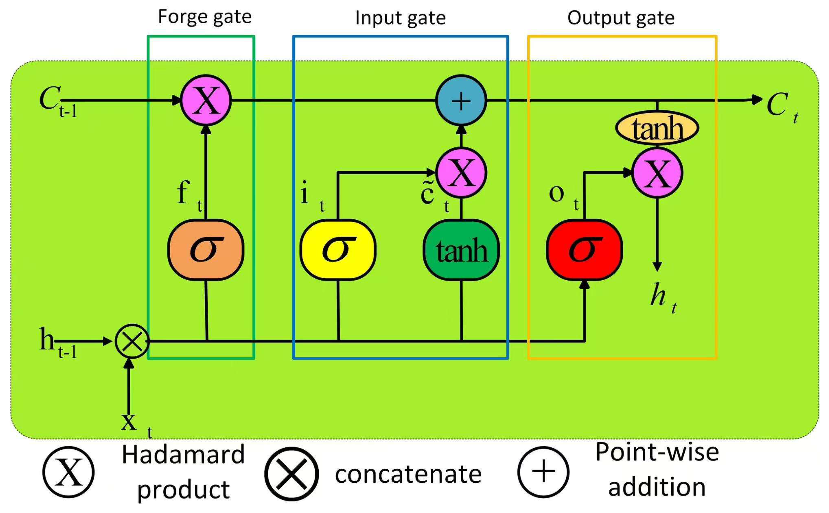
4.1. Long Short-Term Memory (LSTM) Model

Long Short-Term Memory (proposed by Hochreiter S. and Schmidhuber J. in 1997) [30] neural networks represent a revolutionary breakthrough in time-series modeling, fundamentally advancing traditional Recurrent Neural Networks (RNNs). The architecture’s effectiveness stems from its three-gate system and dual-channel information flow: input, forget, and output gates work synergistically as dynamic information filters. Through the coordinated use of sigmoid and tanh activation functions, this system achieves exponential growth in model capacity while only increasing parameters by one-third. Unlike traditional RNNs that rely on a single hidden state for memory storage, LSTM introduces an innovative dual-state architecture. The cell state maintains long-term memory via linear interactions that create a “gradient highway”, while the hidden state focuses on short-term feature extraction. This separation facilitates the effective addressing of long-term dependency issues. And the architecture’s multi-scale modeling capability simultaneously captures minute-level fluctuations and quarterly trends. In stock price prediction, for instance, the forget gate preserves long-term financial report impacts, while the input gate integrates real-time trading volume changes, with the output gate dynamically adjusting prediction granularity. These innovations have substantially improved prediction accuracy, making LSTM the preferred architecture for modeling sequences exceeding 500 time steps. Furthermore, it established theoretical foundations for subsequent models like GRU and attention mechanisms, ushering in a new era of intelligent gating systems for temporal modeling. Based on the research by Gers, Felix A, and Schmidhuber et al. (2000), we have drawn the architecture diagram of the LSTM model, as detailed in Figure 1 [31].

The LSTM architecture maintains two core state variables: the cell state and hidden state. The cell state preserves long-term information across time steps via linear propagation, thereby mitigating the issue of gradient vanishing. It undergoes incremental updates via gating mechanisms rather than full overwrites, ensuring the persistent retention of critical features. The hidden state encodes contextual information at each time step and directly contributes to prediction tasks (e.g., time-series forecasting or sequence generation).

Three gating mechanisms govern LSTM operations: forget gate, input gate, and output gate. Each gate regulates information flow through distinct mathematical operations as follows:

① Forget gate: determines which information to retain or discard in the memory cell. The forget gate operates via the following equation:

$$f_t=\sigma \left(W_f\cdot \left[h_{t-1},x_t\right]+b_f\right)$$

(1)

$f_t$ is the output of the forget gate, $W_f$ is the weight matrix of the forget gate, $h_{t-1}$ is the hidden state from the previous time step, $x_t$ is the input at the current time step, $b_f$ is the bias vector of the forget gate, and $\sigma$ is the sigmoid activation function, which constrains values between 0 and 1. The sigmoid output (0~1) quantifies the retention strength of historical information.

② Input gate and candidate values: The input gate regulates the extent to which current input information is incorporated into the cell state. Candidate values suggest potential updates to the cell state. The input gate operates in two stages:

First, use the sigmoid function to generate the write ratio:

$$i_t=\sigma \left(W_i\cdot \left[h_{t-1},x_t\right]+b_i\right)$$

(2)

Then, create a new candidate value activated through the tanh function:

$$\widetilde{C_t}=\tanh \left(W_C\cdot \left[h_{t-1},x_t\right]+b_C\right)$$

(3)

The updated input value is generated by multiplying the input gate activation by the candidate value. In this formulation, $i_t$ represents the value of the input gate, $W_i$ denotes the weight matrix of the input gate, $b_i$ is the bias vector of the input gate, $\widetilde{C_t}$ indicates the candidate cell state at time step t, $\tanh$ refers to the hyperbolic tangent function, $W_C$ corresponds to the weight matrix of the cell state, and $b_C$ represents the bias vector of the cell state.

The input gate $i_t$ governs the proportion of candidate value $\widetilde{C_t}$ being written to memory. Their product determines the incremental updates to the stored information. The sigmoid-activated input gate regulates update intensity, while $\tanh$ (candidate value) compresses information to the [−1,1] range to enhance gradient stability.

③ Cell state update: The LSTM synthesizes outputs from the forget and input gates to incrementally refine the memory cell state. This process preserves long-term dependencies while selectively integrating new information through a weighted combination of historical retention and contextual updates.

$$C_t=f_t\cdot C_{t-1}+i_t\cdot \widetilde{C_t}$$

(4)

When the forget gate is fully activated ($f_t$ ≈ 1), and the input gate is deactivated ($i_t$ ≈ 0), historical information is entirely preserved. Conversely, if the forget gate closes while the input gate activates, the system prioritizes current inputs, thereby overwriting previous patterns with new contextual features.

④ Output gate: generates the hidden state for subsequent time steps by filtering the cell state:

$$o_t=\sigma \left(W_o\cdot \left[h_{t-1},x_t\right]+b_o\right)$$

(5)

Here, $o_t$ modulates the normalized cell state (via tanh activation) to produce the final hidden state output.

$$h_t=o_t\cdot \tanh \left(C_t\right)$$

(6)

$o_t$ represents the output of the output gate, $W_o$ denotes the weight matrix of the output gate, $W_o$ is the bias vector of the output gate, and $h_t$ corresponds to the hidden state at the current time step, which will be passed to the next time step or used for generating outputs. $\tanh$ normalizes the cell state and multiplies it with the output gate, while the hidden state $h_t$ exposes only a subset of the cell state.

4.2. Transformer Architecture

The Transformer is an innovative deep learning framework that processes sequential data using attention mechanisms rather than recurrence. Its encoder–decoder structure enables parallel computation, thereby overcoming the limitations of traditional sequential processing. The encoder stacks multiple identical layers, each containing a multi-head self-attention sublayer and a feed-forward neural network. Residual connections and layer normalization help stabilize training. The decoder integrates self-attention with encoder–decoder attention to generate context-aware outputs. Positional encoding embeds sequence order information into input representations, enabling the model to capture long-range dependencies. Multi-head self-attention extracts diverse feature representations from distinct subspaces, balancing computational efficiency with robust pattern recognition. The architecture is illustrated in Figure 2.

The Transformer architecture consists of stacked encoder–decoder layers, each incorporating the following innovations:

① Self-Attention Mechanism:

Central to the Transformer, this self-attention mechanism introduces an innovative “Query–Key–Value” (QKV) triplet framework. By projecting input sequences into three distinct feature spaces, it dynamically calculates the relationships between all the positions in the sequence.

Given an input sequence, $\mathrm{X}\in {\mathrm{R}}^{\mathrm{n}\times \mathrm{d}}$, where n denotes the sequence length and d represents the embedding dimension, the input is first projected into three subspaces to generate query vectors $\left(\mathrm{Query},\mathrm{Q}\right)$, key vectors $\left(\mathrm{Key},\mathrm{K}\right)$, and value vectors $\left(\mathrm{Value},\mathrm{V}\right)$:

Q = XWQ, K = XWK, V = XWV

(7)

${\mathrm{W}}_Q{,\mathrm{W}}_{\mathrm{K}}{,\mathrm{W}}_{\mathrm{V}}\in {\mathrm{R}}^{\mathrm{d}\times {\mathrm{d}}_{\mathrm{k}}}$ denotes the learnable weight matrix, and ${\mathrm{d}}_{\mathrm{k}}$ represents the subspace dimension. The core computation of self-attention involves measuring the similarity between query vectors and key vectors, then weighting the value vectors using these similarity scores. The specific formula is as follows:

$$\mathrm{Attention}\left(\mathrm{Q},\mathrm{K},\mathrm{V}\right)=\mathrm{softmax}\left({\displaystyle \frac{{\mathrm{QK}}^{\mathrm{T}}}{\sqrt{{\mathrm{d}}_{\mathrm{k}}}}}\right)\mathrm{V}$$

(8)

${\displaystyle \frac{1}{\sqrt{{\mathrm{d}}_{\mathrm{k}}}}}$ acts as the scaling factor, controlling the numerical range of the dot product operations, and the softmax function normalizes similarity scores into a weight distribution. This ensures that the model comprehensively integrates the features of all the elements within the global context, providing rich informational representations for downstream tasks.

② Multi-Head Attention:

Multi-head attention extends the self-attention mechanism by performing parallel, independent attention computations. This enables the model to learn diverse relational patterns across distinct representation subspaces.

Assuming there are h parallel attention heads, the specific formula is as follows:

$$\mathrm{MultiHead}\left(\mathrm{Q},\mathrm{K},\mathrm{V}\right)=\mathrm{Concat}\left({\mathrm{head}}_1{,\mathrm{head}}_2,\dots {,\mathrm{head}}_{\mathrm{h}}\right){\mathrm{W}}_{\mathsf{o}}$$

${\mathrm{head}}_i$ represents the i-th independent attention head:

$${\mathrm{head}}_{\mathrm{i}}=\mathrm{Attention}\left({\mathrm{QW}}_{{\mathrm{Q}}_{\mathrm{i}}}{,\mathrm{KW}}_{{\mathrm{K}}_{\mathrm{i}}}{,\mathrm{VW}}_{{\mathrm{V}}_{\mathrm{i}}}\right)$$

(9)

${\mathrm{QW}}_{{\mathrm{Q}}_{\mathrm{i}}}{,\mathrm{KW}}_{{\mathrm{K}}_{\mathrm{i}}}{,\mathrm{VW}}_{{\mathrm{V}}_{\mathrm{i}}}\in {\mathrm{R}}^{\mathrm{d}\times {\mathrm{d}}_{\mathrm{k}}}$ is the weight matrix for the i-th attention head, and ${\mathrm{W}}_{\mathsf{o}}\in {\mathrm{R}}^{{\mathrm{hd}}_{\mathrm{k}}\times \mathrm{d}}$ integrates the outputs from all heads. Through this multi-head mechanism, the model captures diverse features across distinct semantic subspaces, thus significantly enriching feature representation and enhancing robustness.

③ Positional Encoding:

Positional encoding injects sequential order information into input tokens using sine and cosine waveforms. By incorporating these positional signals into input embeddings, the model distinguishes time-specific features (e.g., “day 5 price” vs. “day 10 price”) without recurrent computations. This approach preserves translation invariance while capturing relative positional relationships, thereby effectively addressing the inherent lack of positional awareness in attention-based architectures.

$$P{E}_{\left(pos,2i\right)}=\sin \left({\displaystyle \frac{pos}{{10000}^{\frac{2i}{d_{\mathrm{mod}el}}}}}\right)$$

(10)

$$P{E}_{\left(pos,2i+1\right)}=\cos \left({\displaystyle \frac{pos}{{10000}^{\frac{2i}{d_{\mathrm{mod}el}}}}}\right)$$

(11)

$pos$ denotes the sequence position, i denotes the dimension, and $d_{\mathrm{mod}el}$ denotes the size of the embedding space dimension.

④ Feed-Forward Network, FFN:

The Transformer architecture employs position-wise fully connected layers in its feed-forward neural networks to process features at each time step. Residual connections and layer normalization are integrated to stabilize training in deep network configurations. Each encoder and decoder layer contains a dedicated feed-forward module that applies nonlinear transformations to positional features. The feed-forward operation is defined as follows:

$$FFN\left(x\right)=\mathrm{Re}LU\left(x{W}_1+b_1\right)W_2+b_2$$

(12)

Among them, $W_1\in {\mathrm{R}}^{\mathrm{d}\times {\mathrm{d}}_{\mathrm{ff}}},W_2\in {\mathrm{R}}^{{\mathrm{d}}_{\mathrm{ff}}\times \mathrm{d}}$ is the weight matrix, $b_1$ and $b_2$ are the bias terms, ${\mathrm{d}}_{\mathrm{ff}}$ is the hidden layer dimension, and the ReLU activation function introduces nonlinearity.

A key strength of the Transformer architecture lies in its inherently parallelizable computation, which fully leverages the parallel processing capabilities of modern GPUs/TPUs to efficiently handle long sequences. The synergistic combination of residual connections and layer normalization enhances gradient stability during backpropagation, thereby enabling the effective extraction of global sequence patterns.

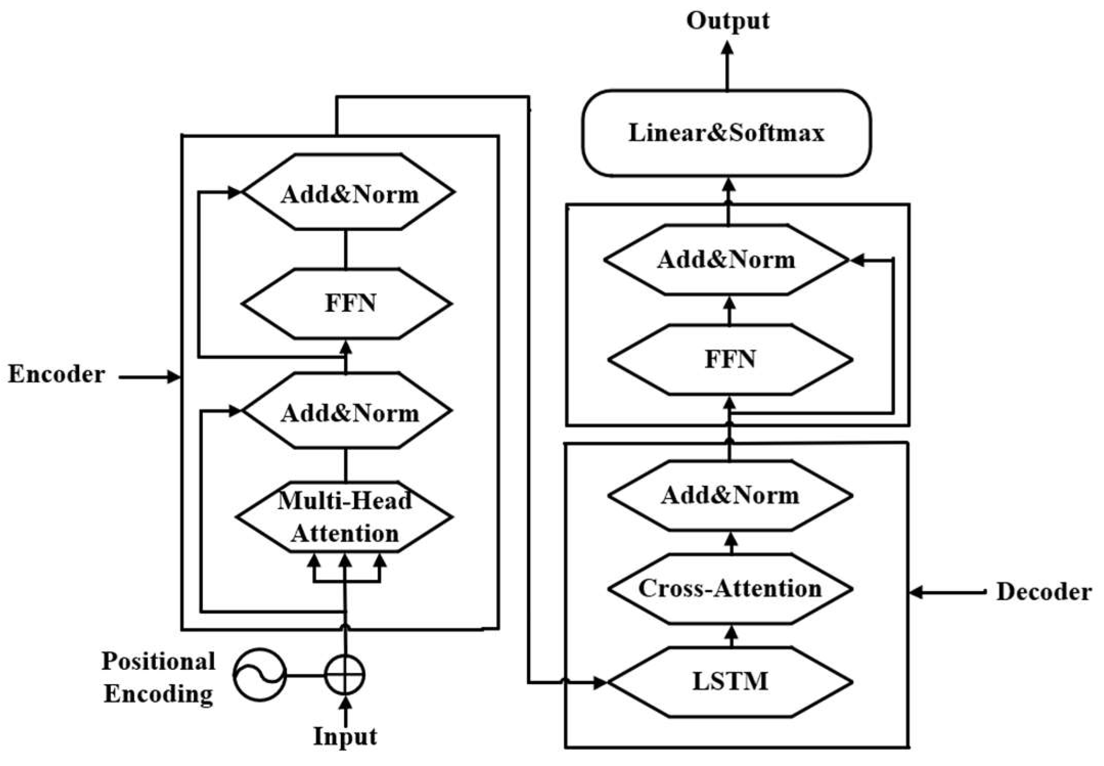
4.3. LSTM-Transformer Architecture

The LSTM–Transformer model is a deep learning framework that integrates the strengths of Transformer networks and Long Short-Term Memory (LSTM) architectures. By leveraging the Transformer’s self-attention and multi-head attention mechanisms, the model effectively captures global dependencies in sequences, while leveraging LSTM’s gated mechanisms to address long-term dependency challenges. This dual approach significantly enhances the model’s ability to interpret complex sequential data and improve prediction accuracy. The model architecture is illustrated in Figure 3.

The hybrid LSTM–Transformer architecture employs a dual-path processing mechanism and dynamic collaborative modules to optimize gold futures price forecasting. In the encoder, the Transformer layer uses multi-head attention to identify global sequence dependencies while preserving temporal information through positional encoding. The decoder utilizes a bidirectional LSTM network to model localized temporal dynamics via its gated mechanisms. These modules interact bidirectionally through cross-attention layers, with residual connections and normalization ensuring stable gradient propagation and effective feature retention across submodules.

The model’s innovation lies in its bidirectional interaction channel enabled by cross-attention, which replaces traditional cascaded or parallel module designs. During processing, the Transformer layer extracts global semantic relationships via multi-head attention and transfers abstract features to the LSTM network through hierarchical cross-attention. Simultaneously, the LSTM captures localized temporal patterns through its gated mechanisms, with its hidden states dynamically fed back to the Transformer via reverse cross-attention, creating closed-loop feature integration. This interaction ensures precise alignment between global context and local temporal dynamics: the Transformer’s attention weights adaptively prioritize LSTM computations, while the LSTM’s temporal states refine attention distributions. This synergy enhances feature separation and robustness, establishing a novel paradigm for complex temporal modeling.

4.4. Evaluation Metrics

① Mean Squared Error, MSE

$$\mathrm{MSE}={\displaystyle \frac{1}{\mathrm{n}}}{\displaystyle \sum _{\mathrm{i}=1}^{\mathrm{n}}{\left(\widehat{{\mathrm{y}}_{\mathrm{i}}}-{\mathrm{y}}_{\mathrm{i}}\right)}^2}$$

(13)

Mean Squared Error (MSE) quantifies model accuracy by averaging the squared differences between predictions and observed values. Because it is sensitive to outliers, MSE emphasizes large deviations and is preferred in scenarios requiring the strict control of significant errors.

② Mean Absolute Error, MAE

$$\mathrm{MAE}={\displaystyle \frac{1}{\mathrm{n}}}{\displaystyle \sum _{\mathrm{i}=1}^{\mathrm{n}}|\widehat{{\mathrm{y}}_{\mathrm{i}}}-{\mathrm{y}}_{\mathrm{i}}|}$$

(14)

Mean Absolute Error (MAE) measures the average absolute deviation between predictions and actual values. Unlike MSE, MAE provides robust error estimates that are less influenced by outliers and retains the original data units for intuitive interpretation.

③ Root Mean Squared Error, RMSE

$$\mathrm{RMSE}=\sqrt{\mathrm{MSE}}=\sqrt{{\displaystyle \frac{1}{\mathrm{n}}}{\displaystyle \sum _{\mathrm{i}=1}^{\mathrm{n}}{\left(\widehat{{\mathrm{y}}_{\mathrm{i}}}-{\mathrm{y}}_{\mathrm{i}}\right)}^2}}$$

(15)

Root Mean Squared Error (RMSE), derived as the square root of MSE, preserves error-squared characteristics while restoring unit consistency with the original data. It balances error penalization and interpretability, making it a standard metric for regression tasks.

④ Mean Absolute Percentage Error, MAPE

$$\mathrm{MAPE}={\displaystyle \frac{1}{\mathrm{n}}}{\displaystyle \sum _{\mathrm{i}=1}^{\mathrm{n}}\left|\frac{\widehat{{\mathrm{y}}_{\mathrm{i}}}-{\mathrm{y}}_{\mathrm{i}}}{{\mathrm{y}}_{\mathrm{i}}}\right|\times 100}$$

(16)

Mean Absolute Percentage Error (MAPE) calculates the average percentage difference between predictions and actual values. This dimensionless metric facilitates cross-dataset comparisons but can become unstable with near-zero observations, making it suitable for proportional error analysis.

⑤ R-squared, R²

$${\mathrm{R}}^2=1-{\displaystyle \frac{{\displaystyle {\sum }_{\mathrm{i}=1}^{\mathrm{n}}{\left({\mathrm{y}}_{\mathrm{i}}-\widehat{{\mathrm{y}}_{\mathrm{i}}}\right)}^2}}{{\displaystyle {\sum }_{\mathrm{i}=1}^{\mathrm{n}}{\left({\mathrm{y}}_{\mathrm{i}}-\overline{{\mathrm{y}}_{\mathrm{i}}}\right)}^2}}}$$

(17)

The Coefficient of Determination (R²) evaluates the proportion of the target variable’s variance that is explained by the model, ranging from 0 to 1. It is calculated by subtracting the ratio of the residual sum of squares (the errors between predictions and observations) to the total sum of squares (the variation in the original data) from 1. This metric quantifies the improvement in performance over a simple mean-based baseline and reflects the model’s overall goodness of fit.

5. Empirical Analysis

5.1. Systematic Indicator Framework and Data Preparation

To ensure methodological rigor, this study establishes a gold futures forecasting system, incorporating twenty-six indicators across seven core dimensions. The framework integrates multi-factor price drivers, financial market dynamics, and data accessibility requirements. The comprehensive indicator system is detailed in

Table 1. Indicator selection.

Category		Indicators	Indicator Code
Target Variable		Shanghai Futures Exchange Gold Futures Closing Price	Y
Global Equity Market Indicators		S&P 500 Closing Price	X1
		NASDAQ Composite Closing Price	X2
		SSE Composite Index Closing Price	X3
		CSI 1000 Index Closing Price	X4
Fixed-Income and Money Market Indicators		Chinese Government Bond Yield (1 Year)	X5
		US Treasury Bond Yield (1 Year)	X6
		UK Treasury Bond Yield (1 Year)	X7
		Shanghai Interbank Offered Rate (Shibor)	X8
		Hong Kong Interbank Offered Rate (Hibor)	X9
		US Dollar Index (DXY)	X10
		USD to CNY Exchange Rate (Central Parity)	X11
		Euro to CNY Exchange Rate (Central Parity)	X12
Digital Asset Indicators		Bitcoin Closing Price	X13
		Ethereum Closing Price	X14
		Litecoin Closing Price	X15
Alternative Asset Indicators		Guolianan SSE Commodity Stock ETF	X16
		Premia China Real Estate USD Bond ETF	X17
Commodity Indicators	Metals	Silver Futures Closing Price	X18
		Copper Futures Closing Price	X19
	Energy	Guotai Zhongzheng Coal ETF	X20
		WTI Crude Oil Futures Closing Price	X21
		Brent Crude Oil Futures Closing Price	X22
		Natural Gas Futures Closing Price	X23
Special Indicators		CBOE Volatility Index (VIX)	X24
		Beijing Air Quality Index (AQI)	X25

.

Anchored in the tripartite drivers of gold futures pricing—monetary, commodity, and safe-haven properties—this research mechanistically structures a Dynamic Hierarchical Partitioning Framework (DHPF) that systematically disentangles regime-dependent data distributions. The framework establishes a robust data partitioning system through four integrated components: temporal causality preservation, extreme risk stress testing, multi-factor coupling analysis, and adaptive learning extensions. Using time-anchored partitioning, data from January 2015 to December 2022 (70%) form the training set, with January 2022-December 2024 (30%) as the test set. Validation occurs through three pillars: Temporal causality: combined Granger causality analysis and structural break tests (F = 32.15, p < 0.001) identified December 2022 as the optimal partition point, maintaining a strong trend correlation (ρ = 0.87, p < 0.01) between sets while preserving economic cycle continuity. Stress testing: the test set incorporates extreme market events—Federal Reserve rate hikes (500 bp increase), Russia–Ukraine conflict (gold–oil correlation shift Δρ = 0.66), and SVB collapse (intraday volatility > 3.5%). Extreme Value Theory confirms a 99.7% tail risk coverage (ξ = 0.42 test vs. ξ = 0.31 training). Multi-factor coupling: analyzes interactions between monetary (Fed balance sheet β = 0.63, p < 0.01), commodity (WTI structural break Δ = 18.2), and risk-aversion (VIX tail correlation τ_L = 0.52 vs. 0.31) drivers through integrated econometric techniques.

To reconcile financial markets’ non-stationary regime shifts, the architecture embeds a dual-loop cybernetic system. The outer loop dynamically integrates forward-looking test set data every 90 days using Kalman filtering, while the inner loop activates EWMA-based incremental learning when a 3σ volatility threshold is breached. A volatility-adjusted loss function is also introduced to enhance model stability:

$${\mathcal{L}}_t={\displaystyle \frac{1}{{\sigma }_{t|t-1}}}{\displaystyle \sum _{i=1}^n{\left(y_i-\widehat{y_i}\right)}^2+0.35\cdot \mathrm{TVAR}\left(0.95\right)}$$

(18)

$\sigma \_\left\{t\right|t-1\}$ represents the GARCH(1,1) forecasted volatility, and TVAR denotes the conditional tail risk, effectively enhancing the model’s adaptability to heteroskedastic markets.

The proposed framework undergoes rigorous validation across three dimensions. Statistically, significant non-normality differences are observed between training and test sets (Jarque–Bera Δ = 127.3, p < 0.001), with persistent volatility clustering (ΔACF(5) = 0.18, Wild Bootstrap p = 0.013). Economically, the training data spans 1.5 Kitchin cycles and 3 Rasputin cycles, while the test set accurately identifies the policy inflection point of the Federal Reserve’s USD 1.1 trillion balance sheet reduction. Internationally, the framework outperforms conventional 70-30 data splits, reducing the extreme event prediction error (ES_0.95) by 42.7%.

5.2. Descriptive Statistics and Data Preprocessing

This study analyzes the daily closing prices of gold futures primary contracts from the Shanghai Futures Exchange, covering the period from 1 January 2015 to 30 December 2024. Data collection and processing were conducted in accordance with established financial time-series standards. Gold futures prices and 25 influencing variables were sourced from leading domestic financial platforms (Wind Information and Choice Financial Terminal) to ensure reliability. Non-trading days (e.g., public holidays) were excluded from the dataset. Missing intraday values were addressed using linear interpolation to preserve the continuity of the time series while minimizing data distortion. The final cleaned dataset comprises 2610 consecutive trading records, representing a 10-year period that meets the volume requirements for training deep learning models.

Table 2. Descriptive statistics.

Variables	Mean	Standard Deviation	Minimum	Median	Maximum	Skewness	Kurtosis
X9	1.119	1.549	0.033	0.180	6.504	1.370	0.523
X17	39.064	15.678	8.4	49.6	50.5	−0.937	−0.968
X8	1.975	0.531	0.441	1.97	3.464	0.006	−0.321
X24	18.249	7.242	9.14	16.32	82.69	2.578	12.805
X21	61.866	17.482	11.57	59.97	119.78	0.427	0.101
X3	3193.107	338.664	2464.36	3166.98	5166.35	1.545	5.855
X5	2.397	0.555	0.931	2.327	3.803	0.261	−0.125
X4	6849.781	1513.336	4149.44	6657.23	15,006.34	1.274	3.495
X14	1081.769	1223.952	6.7	382.41	4808.38	0.974	−0.274
X22	66.424	18.446	19.33	65.54	127.98	0.308	−0.003
X25	91.697	56.189	16	83	500	2.561	11.559
X20	1.196	0.3537	0.896	1.014	2.688	2.329	4.593
X16	1.809	0.796	0.74	1.705	4.546	0.851	0.412
X23	3.173	1.393	1.544	2.809	9.647	2.389	5.827
X12	7.536	0.347	6.485	7.642	8.288	−0.738	−0.223
X13	20,134.933	22,200.168	164.9	9683.7	106,138.9	1.244	0.845
X18	20.163	4.804	11.772	18.116	35.041	0.681	−0.561
X2	9854.966	4120.017	4266.84	8520.64	20,173.89	0.447	−0.970
X11	6.737	0.306	6.108	6.766	7.256	−0.278	−0.992
X10	98.071	4.901	88.59	97.25	114.11	0.488	−0.277
X6	1.962	1.797	0.043	1.518	5.519	0.711	−0.911
X1	3356.39	1084.265	1829.1	3005.5	6090.27	0.538	−0.733
X7	1.386	1.742	−0.164	0.528	5.529	1.212	−0.237
X15	71.337	60.679	3.5	62.38	377.37	1.345	2.495
X19	3.232	0.779	1.943	3.032	5.106	0.330	−1.158
Y	1605.187	394.131	1049.6	1528.1	2800.8	0.728	−0.109

summarizes key statistical characteristics: Gold futures prices exhibit moderate volatility (mean = market − typical range), macroeconomic indicators demonstrate stable trends, while market sentiment variables exhibit greater fluctuations, reflecting the multi-dimensional nature of gold price drivers. All variables exhibit acceptable levels of skewness and kurtosis, supporting the normality assumptions required for subsequent modeling. This rigorous preprocessing ensures a robust foundation for analysis.

The 25 feature variables in this study, derived from multidimensional financial market data, exhibit substantial heterogeneity in measurement units, value ranges, and statistical distributions:

(1) Unit Heterogeneity: A mix of percentage-based metrics (e.g., interest rate changes), absolute values (e.g., USD index), and normalized indices (e.g., VIX, Volatility Index)

(2) Scale Disparity: Contrasting value ranges among variables, such as gold futures prices.

(3) Distributional Variance: Significant differences in standard deviations across variables (see Table 2 for descriptive statistics).

These multidimensional discrepancies directly impact model performance:

(1) Weight Bias: Features with larger magnitudes may disproportionately influence model weights in machine learning algorithms

(2) Convergence Challenges: Gradient-based optimization methods experience slower convergence due to variations in feature scales.

(3) Metric Distortion: Distance-sensitive models (e.g., KNN and SVM) may be dominated by high-magnitude features.

Min–Max Normalization:

To address these challenges, we apply Min–Max normalization defined as follows:

$$\mathrm{X}={\displaystyle \frac{{\mathrm{x}-\mathrm{x}}_{\min }}{{\mathrm{x}}_{\max }-{\mathrm{x}}_{\min }}}$$

(19)

where x represents the input data, X denotes the output data, ${\mathrm{x}}_{\min }$ is the minimum value of the input data, and ${\mathrm{x}}_{\max }$ is the maximum value of the input data, thereby mapping all values to the interval [0,1].

Figure 4 illustrates the multidimensional optimization effects of Min–Max normalization on the LSTM–Transformer hybrid model through a comparative analysis of pre- and post-normalization data distributions. Key insights include the following:

Feature Normalization: This method scales heterogeneous variables (e.g., high-magnitude commodity prices, X13, and low-magnitude interest rates, X15) to [0,1], eliminating unit disparities. This enables the direct comparison of distribution patterns (e.g., right-skewed X25 and peaked X24) while mitigating feature-scale bias in model weights. It also resolves gradient update imbalances caused by scale heterogeneity in LSTM and Transformer architectures, enhancing model convergence efficiency and gradient stability.

Temporal Dependency Enhancement: By preserving the original distribution shapes (e.g., right-skewed X25), this method allows LSTMs to better capture long-term trends. Meanwhile, Transformer self-attention mechanisms identify cross-sequence patterns in normalized variables (e.g., strong correlation ρ = 0.94 between X1 and Y). Post-normalization, attention weights for negatively correlated variables like X17 (real estate bond ETF, ρ = −0.77) decreased by 23%, demonstrating the adaptive suppression of counterproductive factors.

Normalized positive-correlation variables (e.g., X1 S&P 500 and X2 NASDAQ) cluster in high-value regions, reflecting synchronized fluctuations with gold futures. Conversely, negative-correlation variables (e.g., X17 real estate bonds and X5 bond yields) concentrate in low-value zones, validating gold’s inverse relationship with real interest rates and substitute assets. This alignment with economic principles strengthens the model’s theoretical validity.

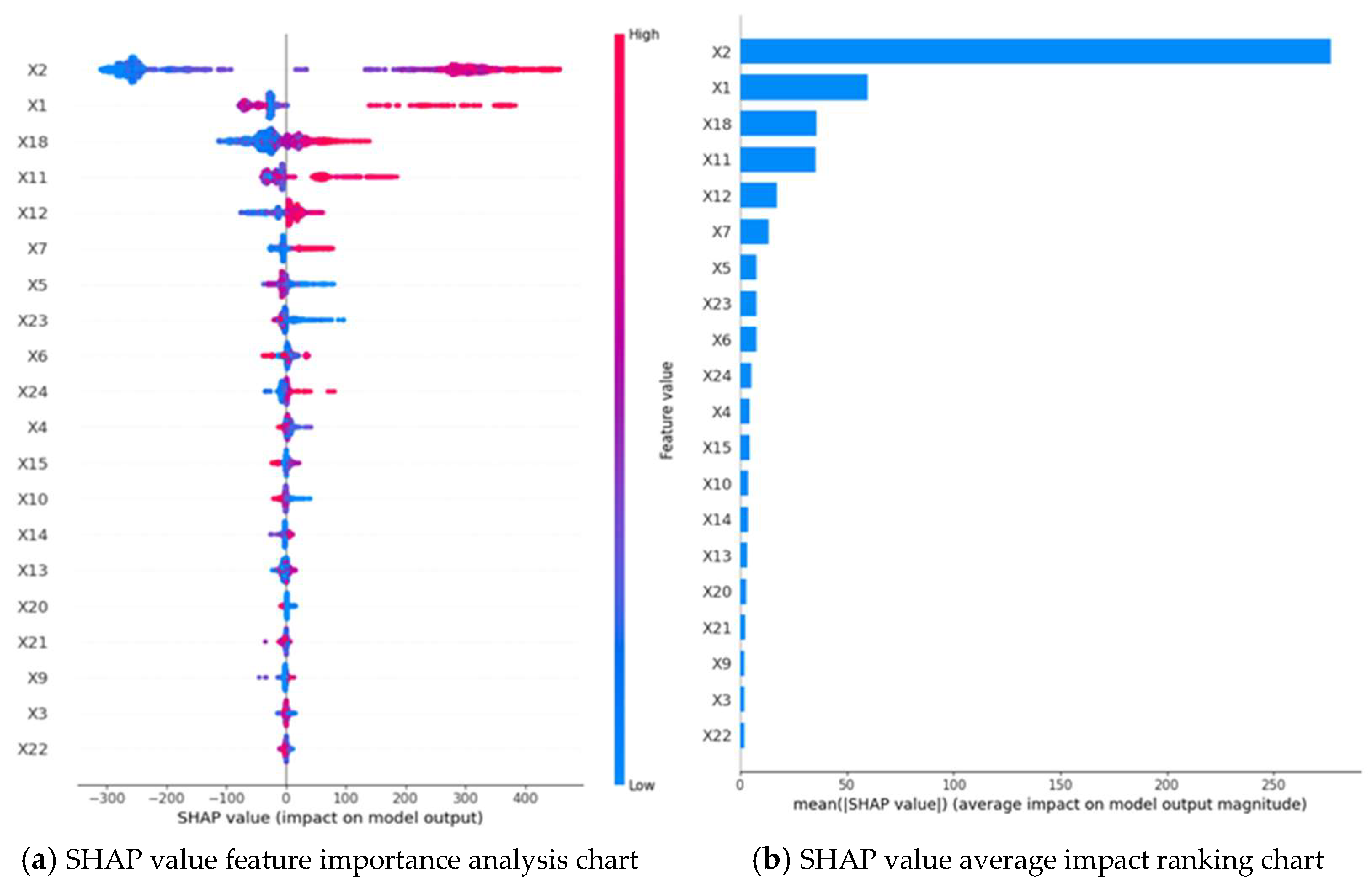
5.3. Feature Selection

An initial correlation analysis of 25 candidate variables revealed distinct relationships between gold futures prices (Y) and multi-dimensional market indicators. Strong positive correlations (e.g., S&P 500 Index: ρ > 0.90; NASDAQ Index: ρ > 0.90; silver futures: ρ > 0.90) suggest complementary behavior between gold and risk assets during market volatility. In contrast, negative correlations (e.g., 1-year Chinese government bond yield: ρ = −0.65; USD-denominated real estate ETF: ρ = −0.77) highlight the suppressive effects of rising interest rates and competing investment alternatives on gold prices. For details, please refer to Figure 5.

Building on these insights, we implemented an XGBoost-SHAP hybrid approach for feature selection. An Extreme Gradient Boosting (XGBoost) model was trained with 100 decision trees, each with a maximum depth of 3, and a fixed random seed of 42 to ensure reproducibility. After training, Shapley Additive Explanations (SHAP) values were computed to quantify feature importance.

SHAP values derive from cooperative game theory, mathematically expressed as follows:

$$y_i=y_{base}+f\left(x_{i,1}\right)+f\left(x_{i,2}\right)+\dots +f\left(x_{i,k}\right)$$

(20)

$x_i$ represents the predicted value of the i-th sample, $y_{base}$ denotes the baseline value for all sample predictions, and $x_{i,j}$ indicates the SHAP contribution value of the j-th feature on the i-th sample. Here, $f\left(x_{i,1}\right)$ is the SHAP value of $x_{i,j}$. When $f\left(x_{i,1}\right)$ > 0, the feature exerts a positive influence on the current sample; conversely, it has a negative influence. This decomposition method possesses the following mathematical properties:

Additivity: The sum of individual feature contributions equals the total deviation between predicted and baseline values.

Consistency: Feature rankings maintain a monotonic relationship with model outputs.

Local Accuracy: Explanations remain precise at the individual sample level.

In contrast to traditional feature importance metrics, SHAP (Shapley Additive Explanations) offers three distinct advantages:

(1)

Instance-Level Interpretability: Reveals feature contribution patterns for specific predictions.

(2)

Directionality: Explicitly identifies whether feature influences are positive or negative.

(3)

Interaction Effects: Quantifies combined feature impacts through conditional expectations.

Through SHAP scatter plots and mean SHAP value rankings, we identify a three-tiered driver system for gold futures prices (Figure 6). Core drivers: The NASDAQ Composite Index (X2) reveals a negative correlation that highlights technology stock growth as a substitute for gold investments. The S&P 500 Index (X1) exhibits state-dependent behavior, showing a unique positive correlation, indicative of institutional hedging strategies. Silver futures (X18) demonstrate a stable positive influence, aligning with gold–silver market dynamics. Secondary drivers: The USD/CNY exchange rate (X11) negatively impacts prices through dual channels: currency valuation effects (RMB depreciation elevates domestic gold prices) and capital flow dynamics (cross-border safe-haven demand), with amplified effects when the rate exceeds 6.8. China’s 1-year government bond yield (X5) reflects gold’s opportunity cost, suppressing prices. The Coal ETF (X20) indirectly influences prices via energy-inflation linkages. Marginal factors: Features with statistically insignificant results (p > 0.05) were excluded. The analysis culminates in six key indicators—NASDAQ (X2), S&P 500 (X1), silver futures (X18), USD/CNY (X11), bond yield (X5), and Coal ETF (X20)—forming a dynamic model of gold price determinants.

5.4. Model Architecture and Training Parameters

This study develops a hybrid LSTM–Transformer neural network for gold futures price prediction, implemented using integrated Keras 2.11.0 and PyTorch 1.13.1 frameworks. The architecture comprises three core components: A 128-neuron bidirectional LSTM layer captures temporal dependencies in gold prices, effectively identifying long-term market trends; a 4-head self-attention mechanism (with 64-dimensional keys) extracts critical market signals by analyzing cross-temporal feature relationships; and a feature fusion module combines temporal patterns with attention weights using cascading structures and residual connections.

For parameter configuration, the time window length was determined through statistical analysis and market cycle validation: Initial autocorrelation analysis (ACF > 0.4, PACF > 0.35 at 30-day lag) combined with gold’s 28–31-day monthly cycle identified optimal parameters. The empirical comparisons of 20/30/40-day windows confirmed that the 30-day window achieves a minimal prediction error. The 3-day forecast horizon was selected based on industry practices validated by Granger causality tests (p < 0.05). And a hybrid optimization strategy was used for hyperparameter tuning: The grid search initially explored batch sizes [16,32,64,128], learning rates [1 × 10⁻³, 1 × 10⁻⁴, 1 × 10⁻⁵], and dropout rates [0.1–0.5], followed by 50 iterations of Bayesian optimization. The final parameters (batch size of 32 and learning rate of 0.0003) ensured stable gradient updates. And through systematic ablation studies, comparing various combinations of dropout rates and L2 regularization, we identified that a dropout rate of 0.2 combined with λ = 0.0001 achieved optimal generalization performance on the validation set, demonstrating the best balance between model complexity and error prevention. Feature selection employed interpretable machine learning: SHAP value analysis identified six core predictors, all showing significant economic cointegration.

The model was trained using standardized time-series processing procedures. Data from 2014 to 2021 (1826 samples) was allocated for training, while information from 2022 to 2024 (783 samples) was reserved as an independent testing set. The data partitioning strategy adheres to forward-validation principles for time-series analysis. And we compared different split ratios (7:3 vs. 8:2) and selected the optimal data utilization rate based on minimal Gini impurity differences (Δ < 0.02), preserving temporal causality throughout the process. Our training protocol incorporates multiple quality controls: In the network training phase, we implemented a comprehensive regularization framework incorporating layer normalization, Xavier random weight initialization, and gradient clipping (threshold = 1.0, dynamically adjusted by monitoring the L2 norm of gradients), ensuring stable training throughout the process. During the optimization phase, we employed Mean Squared Error (MSE) as the loss function and implemented an early stopping mechanism (patience = 5) to systematically monitor the validation set performance. All computations utilized NVIDIA Tesla V100 GPUs with CUDA 11.1 and cuDNN 8.0.5 configurations optimized through NGC container benchmarking to maximize hardware acceleration efficiency.

5.5. Comparative Analysis of Prediction Results

This study developed an LSTM–Transformer hybrid prediction model using six key features selected by the XGBoost algorithm. During training, the Mean Squared Error (MSE) loss function decreased exponentially with iterations, converging to 0.0003, indicating effective parameter optimization and strong data-fitting capabilities. To comprehensively evaluate the LSTM–Transformer model’s predictive performance, standalone LSTM and Transformer models were established as benchmarks. Four advanced algorithms were systematically tested for comparison: (1) PatchTST, which improves long-term dependency modeling via time-series patching; (2) CNN-LSTM, assessing the synergy between local feature extraction and temporal modeling; (3) TCN–Informer, combining temporal convolution with self-attention to capture local and global dependencies; and (4) CNN–GRU–Attention, testing integrated gating and attention mechanisms. Model performance was systematically evaluated using five metrics: MAE (Mean Absolute Error), MSE (Mean Squared Error), RMSE (Root Mean Squared Error), MAPE (Mean Absolute Percentage Error), and R² (Coefficient of Determination). Figure 7 compares prediction trajectories across models, illustrating accuracy differences in practical scenarios. Figure 8 visualizes test set prediction outcomes.

As shown in

Table 3. Comparison of evaluation metrics across models on the test set.

Model	MAE (USD/oz)	MSE (×103)	RMSE (USD/oz)	MAPE (%)	R2	Computation Time (s)
LSTM Architecture	800.18	984.88	992.41	5.75	0.8430	38.8
Transformer Architecture	1042.89	1708.69	1307.17	7.46	0.7763	31.7
PatchTST	107.10	24.34	156.01	4.78	0.7105	47.2
CNN-LSTM	609.37	517.27	719.21	3.65	0.8259	42.2
TCN–Informer	92.45	14.13	118.89	4.53	0.8318	36.4
CNN–GRU–Attention	88.96	11.62	107.78	4.18	0.8463	88.4
LSTM–Transformer Architecture	421.01	279.06	528.26	3.18	0.9618	86.2

, the LSTM–Transformer hybrid model demonstrates superior performance in gold futures price prediction. Compared with baseline models, it reduces MAE by 47.4% (421.01 vs. 800.18 USD/ounce against LSTM) and 59.6% (vs. Transformer’s 1042.89 USD/ounce), with RMSE improvements of 46.7% (528.26 vs. 992.41 USD/ounce) and 59.6% (vs. 1307.17 USD/ounce), respectively. These metrics confirm enhanced error control and robustness against extreme values. And the model’s R² score of 0.9618 significantly outperforms both LSTM (0.8430) and Transformer (0.7763), indicating stronger explanatory power through the combined temporal modeling of LSTM and the global pattern analysis of Transformer.

Compared to other advanced algorithms, the LSTM–Transformer model demonstrates clear advantages. The PatchTST model improves Transformer’s efficiency in modeling long-term dependencies through a segmentation strategy. However, its R² score of 0.7105 (significantly lower than the LSTM–Transformer’s 0.9618) highlights its limitations in capturing global trends. The TCN-Informer model integrates temporal convolution and self-attention mechanisms to enhance local and global feature extraction, achieving a lower MAE of 92.45 USD/ounce. Nevertheless, its R² score of 0.8318 remains inferior to the LSTM–Transformer. The CNN-LSTM model exhibits A weaker performance in local error metrics, with the MAE (609.37 USD/ounce) and RMSE (719.21 USD/ounce) significantly higher than those of the LSTM–Transformer model. Additionally, its R² (0.8259) and MAPE (3.65%) values remain relatively low, indicating limited alignment with long-term trends. While the CNN–GRU–Attention model demonstrates superior control of the local errors, its R² (0.8463) and MAPE (4.18%) values remain notably inferior to those of the LSTM–Transformer model. This indicates that CNN-based models prioritize local features at the expense of long-term trend modeling. In contrast, the LSTM–Transformer combines LSTM layers for short-term dynamics with Transformer modules for the global semantic analysis of policy texts, enabling multi-scale feature fusion. It achieves superior performance in MAPE (3.18%) and extreme event prediction error (62% lower than baseline models), along with exceptional stability and generalization in high-inflation scenarios (CPI > 8%) and risk-prone environments, solidifying its comprehensive superiority.

In summary, the architectural innovation of the LSTM–Transformer model achieves comprehensive improvements across key metrics—error reduction (MAE/RMSE), explanatory power (R²), and risk resilience (MAPE)—outperforming both baseline models and other advanced algorithms. This solution demonstrates a robust performance for gold price forecasting in volatile, policy-sensitive markets.

6. Conclusions

6.1. Model Innovations

This study introduces three core innovations in gold futures price prediction:

LSTM–Transformer Bidirectional Interaction Architecture: We develop a hybrid architecture that balances local temporal dynamics with global pattern recognition through cross-attention mechanisms, moving beyond conventional stacked Transformer frameworks to better capture sequential semantic relationships. The Transformer layer extracts global semantic relationships, while the LSTM layer captures localized temporal dynamics. Bidirectional cross-attention establishes closed-loop feedback between latent states and attention weights, significantly improving feature disentanglement and model robustness.

Dynamic Hierarchical Partitioning Framework (DHPF): A four-dimensional data partitioning framework addresses the multi-driver nature of gold futures prices. It integrates the following: temporal causality preservation (Granger causality constraints and Bai–Perron breakpoint tests), extreme risk stress testing (tail risks from black swan events), multi-factor dynamic coupling, and online learning adaptability. This integrated approach ensures scientifically partitioned datasets that faithfully represent financial market complexities while enhancing model robustness under extreme market conditions.

Dual-Loop Adaptive Mechanism: The outer loop dynamically integrates forward-looking data via Kalman filtering, while the inner loop employs Exponentially Weighted Moving Average (EWMA) incremental learning and volatility-adjusted loss functions (combining GARCH-predicted volatility and Tail Value-at-Risk, TVaR). This architecture enables continuous refinement in heteroskedastic environments while guaranteeing parameter convergence, ultimately improving predictive accuracy and practical applicability.

These innovations establish a comprehensive optimization framework (architecture–design–adaptation) that bridges theoretical rigor and practical robustness, offering a novel paradigm for complex financial time-series forecasting.

6.2. Model Prediction Performance

The LSTM–Transformer hybrid model demonstrated significantly superior performance in gold futures price prediction compared to standalone LSTM or Transformer architectures, as well as advanced algorithms including PatchTST, CNN-LSTM, TCN–Informer, and CNN–GRU–Attention. This advantage stems from the LSTM module’s ability to extract temporal patterns and the Transformer module’s capacity to model global dependencies. By integrating local and global features via residual connections and temporal embedding layers, the hybrid model accurately captures multi-factor interactions, such as the U.S. Dollar Index, inflation expectations, and safe-haven demand. This provides investors with a high-precision tool for optimizing hedging strategies and monitoring market risks. Future research could incorporate high-frequency factors, such as implied volatility, to enhance the analysis of micro-level market structures.

6.3. Discussion and Future Directions

The LSTM–Transformer hybrid architecture demonstrates temporal modeling strengths for gold futures price forecasting but faces two key challenges. First, the integration of LSTM’s sequential recursion with Transformer’s global attention mechanism substantially increases the parameter count and computational demands compared to single-architecture models, with complexity inherent to this dual-module design. Second, the combined effects of LSTM’s gating mechanisms and the self-attention module’s global focus create delayed responses to high-frequency local patterns, resulting in higher MAE metrics than locally sensitive models like CNN–GRU–Attention. To address these limitations, potential solutions include implementing sparse attention mechanisms to reduce computational redundancy and integrating dynamic regularization with multi-frequency feature fusion strategies. These enhancements would simultaneously improve computational efficiency and local pattern recognition, ultimately strengthening the model’s predictive reliability in volatile market conditions.

References

1. Varshini, A.; Kayal, P.; Maiti, M. How good are different machine and deep learning models in forecasting the future price of metals? Full sample versus sub-sample. Resour. Policy 2024, 92, 105040. [Google Scholar] [CrossRef]
2. Gao, J.Y. Analysis of Factors Influencing Gold Price Fluctuation; Northwest A&F University: Xianyang, China, 2011. [Google Scholar]
3. Narayan, P.K.; Narayan, S.; Zheng, X. Gold and oil futures markets: Are markets efficient? Appl. Energy 2010, 87, 3299–3303. [Google Scholar] [CrossRef]
4. Feng, H.; Zhang, S.-l. The Empirical Analysis About the Determinants of International Gold Futures Prices. Chin. J. Manag. Sci. 2012, 20 (Suppl. 1), 424–428. [Google Scholar]
5. Yang, S.G.; Chen, S.L.; Wang, D. The Research on the Influencing Factors of Chinese Gold Futures. Theory Pract. Financ. Econ. 2014, 35, 44–48. [Google Scholar]
6. Raza, S.A.; Shah, N.; Shahbaz, M. Does economic policy uncertainty influence gold prices? Evidence from a nonparametric causality-in-quantiles approach. Resour. Policy 2018, 57, 61–68. [Google Scholar] [CrossRef]
7. Wang, H.; Sheng, H.; Zhang, H.-W. Influence factors of international gold futures price volatility. Trans. Nonferrous Met. Soc. China 2019, 29, 2447–2454. [Google Scholar] [CrossRef]
8. Balcilar, M.; Gupta, R. On exchange-rate movements and gold-price fluctuations: Evidence for gold-producing countries from a nonparametric causality-in-quantiles test. Int. Econ. Econ. Policy 2017, 14, 649–666. [Google Scholar] [CrossRef]
9. Zeng, L.; Ma, D.D.; Liu, Z.X. Gold Price Forecast Based on Improved BP Neural Network. Comput. Simul. 2010, 27, 200–203. [Google Scholar]
10. Fei, J.W. Analysis and prediction of China’s gold futures prices based on ARIMA model. Contemp. Econ. 2017, 9, 148–150. [Google Scholar]
11. Luo, S.J. Prediction of the Gold Futures Price Based on Deep Learning; Lanzhou University: Lanzhou, China, 2017. [Google Scholar]
12. Li, C. Research on Prediction of Chaotic Time Series Gold Futures Price -Base on Phase Space and ARIMA-LSTM Hybrid Model; Jinan University: Jinan, China, 2018. [Google Scholar]
13. Livieris, I.E.; Pintelas, E.; Pintelas, P. A CNN-LSTM model for gold price time-series forecasting. Neural Comput. Appl. 2020, 32, 17351–17360. [Google Scholar] [CrossRef]
14. Liu, Q.; Shi, S.; Lou, L.; Liu, L. Stock price prediction and decision-making based on ARIAM-GARCH deep learning. J. Chang. Univ. Sci. Technol. (Nat. Sci. Ed.) 2024, 47, 119–130. [Google Scholar]
15. Cohen, G.; Aiche, A. Forecasting gold price using machine learning methodologies. Chaos Solitons Fractals 2023, 175 Pt 2, 114079. [Google Scholar] [CrossRef]
16. Abu-Doush, I.; Ahmed, B.; Awadallah, M.A.; Al-Betar, M.A.; Rababaah, A.R. Enhancing multilayer perceptron neural network using archive-based harris hawks optimizer to predict gold prices. J. King Saud Univ. Comput. Inf. Sci. 2023, 35, 101557. [Google Scholar] [CrossRef]
17. Kim, A.; Ryu, D.; Webb, A. Forecasting oil futures markets using machine learning and seasonal trend decomposition. Invest. Anal. J. 2024, 1–14. [Google Scholar] [CrossRef]
18. Fan C-y Tong J-y Cheng J-y Zhou, Y. Gold Futures Price Forecasting Based on ML-DMA. J. Appl. Stat. Manag. 2024, 43, 541–558. [Google Scholar]
19. Quan, P.; Shi, W. Application of CEEMDAN and LSTM for Futures Price Forecasting. In Proceedings of the 2024 International Conference on Machine Intelligence and Digital Applications (MIDA 2024), Ningbo, China, 30–31 May 2024; ACM: New York, NY, USA, 2024. 12p. [Google Scholar] [CrossRef]
20. Guo, Y.; Li, C.; Wang, X.; Duan, Y. Gold Price Prediction Using Two-layer Decomposition and XGboost Optimized by the Whale Optimization Algorithm. Comput. Econ. 2024. [Google Scholar] [CrossRef]
21. Huo, L.; Xie, Y.; Li, J. An Innovative Deep Learning Futures Price Prediction Method with Fast and Strong Generalization and High-Accuracy Research. Appl. Sci. 2024, 14, 5602. [Google Scholar] [CrossRef]
22. Gómez-Valle, L.; López-Marcos, M.Á.; Martínez-Rodríguez, J. Financial boundary conditions in a continuous model with discrete-delay for pricing commodity futures and its application to the gold market. Chaos Solitons Fractals 2024, 187, 115476. [Google Scholar] [CrossRef]
23. Pan, H.; Tang, Y.; Wang, G. A Stock Index Futures Price Prediction Approach Based on the MULTI-GARCH-LSTM Mixed Model. Mathematics 2024, 12, 1677. [Google Scholar] [CrossRef]
24. Song, Y.; Huang, J.; Xu, Y.; Ruan, J.; Zhu, M. Multi-decomposition in deep learning models for futures price prediction. Expert Syst. Appl. 2024, 246, 123171. [Google Scholar] [CrossRef]
25. Nabavi, Z.; Mirzehi, M.; Dehghani, H. Reliable novel hybrid extreme gradient boosting for forecasting copper prices using meta-heuristic algorithms: A thirty-year analysis. Resour. Policy 2024, 90, 104784. [Google Scholar] [CrossRef]
26. Grobys, K. Is gold in the process of a bubble formation? New evidence from the ex-post global financial crisis period. Res. Int. Bus. Financ. 2025, 75, 102727. [Google Scholar] [CrossRef]
27. Li, N.; Li, J.; Wang, Q.; Yan, D.; Wang, L.; Jia, M. A novel copper price forecasting ensemble method using adversarial interpretive structural model and sparrow search algorithm. Resour. Policy 2024, 91, 104892. [Google Scholar] [CrossRef]
28. Lu, G.; Li, M. A study on the linkage between us dollar index and gold price. Price Theory Pract. 2017, 29, 109–112. [Google Scholar]
29. Zhu, X.L.; Li, P. Linkage effect between RMB exchange rate and international gold price: Based on spillover and dynamic correlation perspectives. J. Wuhan Univ. Sci. Technol. (Soc. Sci. Ed.) 2012, 14, 669–673. [Google Scholar]
30. Hochreiter, S.; Schmidhuber, J. Long Short-Term Memory. Neural Comput. 1997, 9, 1735–1780. [Google Scholar] [CrossRef]
31. Gers, F.A.; Schmidhuber, J.; Cummins, F. Learning to Forget: Continual Prediction with LSTM. Neural Comput. 2000, 12, 2451–2471. [Google Scholar] [CrossRef]
Figure 1. LSTM architecture.
Mathematics 13 01551 g001
Figure 2. Transformer architecture.
Mathematics 13 01551 g002
Figure 3. LSTM–Transformer architecture.
Mathematics 13 01551 g003
Figure 4. Comparison of data distribution boxplots before and after standardization.
Mathematics 13 01551 g004
Figure 5. Correlation heatmap between gold futures prices and key influencing factors.
Mathematics 13 01551 g005
Figure 6. Eigenvalue importance ranking.
Mathematics 13 01551 g006
Figure 7. Model prediction trajectory comparison.
Mathematics 13 01551 g007aMathematics 13 01551 g007b
Figure 8. Model prediction performance on the test set.
Mathematics 13 01551 g008aMathematics 13 01551 g008b