Transformer and Convolutional Neural Network: A Hybrid Model for Multimodal Data in Multiclass Classification of Alzheimer’s Disease

Abstract

Alzheimer’s disease (AD) is a form of dementia that progressively impairs a person’s mental abilities. Current classification methods for the six AD stages perform poorly in multiclass classification and are computationally expensive, which hinders their clinical use. An efficient, low-computational model for accurate multiclass classification across all AD stages is needed that can integrate both local and global feature extraction. This study uses rs-fMRI, clinical data, and transformer-based models to classify six AD stages. The proposed network is a hybrid of two architectures, namely a transformer and a convolutional neural network (CNN). The model addresses multiclass classification by examining the brain’s functional connectivity networks based on rs-fMRI data and clinical data from the Alzheimer’s Disease Neuroimaging Initiative (ADNI). The proposed architecture leverages CNNs for local feature extraction and transformers for global context; this method employs the contextual attention power of transformers to improve the multiclass classification accuracy of AD. The k-fold cross-validation method was employed to evaluate the performance of the proposed model. For the multiclass classification of six stages, the average accuracy of the model was 96%. For binary classification, accuracies were 98.96% (AD vs. MCI), 99.65% (AD vs. CN), 98.44% (AD vs. LMCI), 96.88% (AD vs. EMCI), and 98.36% (AD vs. SMC). These results highlight the potential of the proposed network in achieving high accuracy for both binary and multistage AD classification with limited computational resources. The proposed method was also compared to benchmark algorithms and outperformed them; it was substantially less computationally expensive while maintaining its accuracy.

1. Introduction

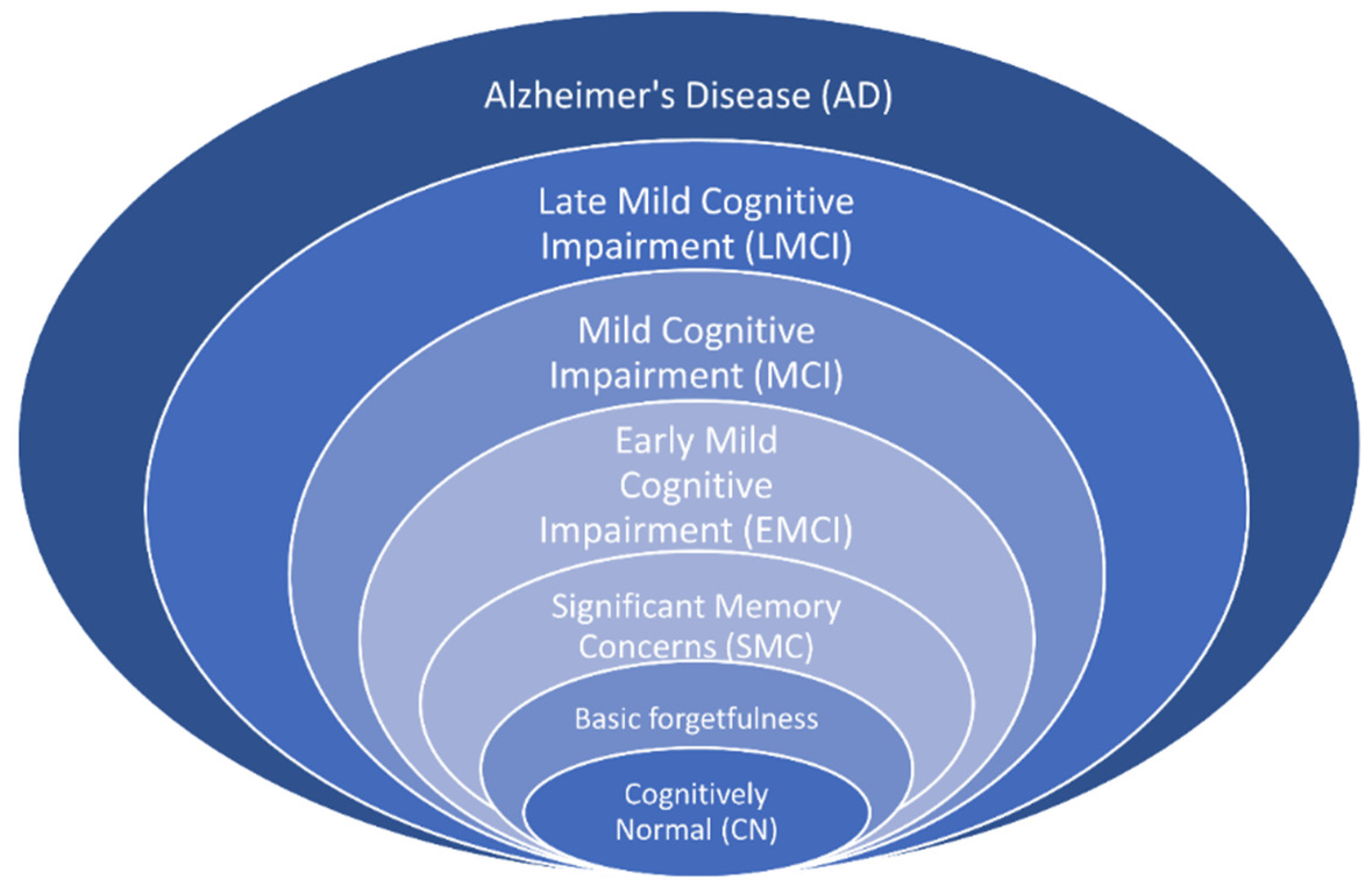
The decline of cognitive senses, such as the ability to think, recall, and reason, to the point where it disrupts routine tasks, is known as dementia. Dementia has more than 400 varieties. Alzheimer’s disease (AD) is one of the most common forms and affects 60–70% of dementia patients [1]. It is unclear what exactly causes this disease, but it is generally related to age: on average, people who have AD are over 65 years old. There are several treatments for AD, but no cure at present. The disease progresses over time from the initial phase to the severe phase, through seven stages: cognitively normal (CN), basic forgetfulness, significant memory concerns (SMC), early mild cognitive impairment (EMCI), mild cognitive impairment (MCI), late mild cognitive impairment (LMCI), and AD, as shown in Figure 1. The CN stage feels like a normal effect of aging. The first two stages can be considered as one, as there is no significant difference between them (https://www.pennmedicine.org/updates/blogs/neuroscience-blog/2019/november/stages-of-alzheimers, accessed on 13 February 2024). The SMC stage is followed by basic forgetfulness and involves some memory issues. The last three stages start to affect daily activities.

MCI is a critical stage, as patients with MCI are relatively likely to be diagnosed with AD. This fact means that identifying EMCI, MCI, and LMCI before AD is crucial. Several alterations in the brain, including the disintegration of functional networks and volume changes, are linked to EMCI. 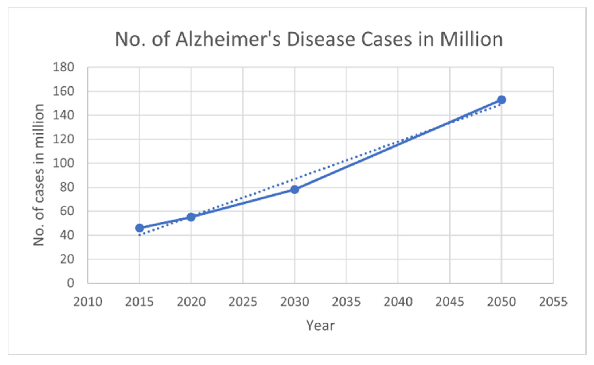Reduced motor, cognitive, and affective functioning results from additional LMCI-related changes in the brain’s cerebellum [2]. According to the World Health Organization (WHO), AD is a relentless and growing global crisis, with over 55 million people affected worldwide; according to the World Alzheimer Report 2019, the number of cases may triple by 2050, as shown in Figure 2 (https://www.alzint.org/resource/world-alzheimer-report-2019/, accessed on 13 February 2024). Each year, nearly 10 million new cases emerge, indicating the disease’s worldwide spread. Economically, AD imposes a vast burden, with global costs exceeding USD 1.3 trillion in 2019, which is anticipated to increase to USD 2.8 trillion by 2030 [3]. This financial burden highlights the catastrophic effects on families and society. Furthermore, there is an emotional cost for people, who provide nearly 18.4 billion hours of unpaid care yearly.

The symptoms of different stages can vary across individuals. K. A. Johnson et al. [4] revealed that the hippocampus, which is a part of the brain accountable for memory and learning, decreased by 10% due to AD. To raise the standard of living for patients and advance prevention and treatment, it is necessary to detect AD in its initial phases and identify its progression. Many neuroimaging techniques can be used for AD diagnosis, including magnetic resonance imaging (MRI), functional MRI (fMRI), fMRI during resting state (rs-fMRI), computerized tomography (CT) scans, positron emission tomography (PET) scans, electroencephalogram (EEG), single-photon emission computed tomography, and magnetoencephalography (MEG) [5]. All these methods are used for diagnosing neuroimaging diseases. However, MRI, CT scan, PET, fMRI, and EEGs are utilized most often.

MRI scans offer precise information about changes in the human brain. fMRI measures the minute changes in blood flow that coincide with brain activity and displays the activity in particular brain regions. Similarly, rs-fMRI data are used to examine intrinsic networks in the brain while the individual is at rest. CT scans involve X-rays that process images of the inside of an organ. This method works best for cancer detection, lung and chest imaging, and bone damage. CT is unsuitable when investigating soft tissue structures, such as the brain. PET scans the body for disease using a radioactive material; the function of tissues and organs can be seen on the PET scan. However, fMRI is clearer than a PET scan and provides a better understanding of the relevant organ [5].

For studying AD and its stages, rs-fMRI is relatively reliable, as it generally involves a non-invasive brain imaging procedure that quantifies neural activity without the use of any stimulus. Such activity is determined by alterations in the blood oxygenation level. Compared to other imaging methods, which are carried out based on the patient’s activity or tasks, rs-fMRI can be used in older people or persons with cognitive impairments, since the measurement is performed without stimulating the patient. This technique is most effective in identifying AD, as it captures minor alterations in the functional connectivity map in the brain, which are usually localized in specific networks. In this regard, rs-fMRI is superior to the other imaging techniques as a diagnostic method for assessing the evolution of AD from MCI to dementia. It detects the illness’s influence on brain activity without requiring invasive procedures and complicated tasks [6]. Apart from neuroimaging data, clinical data and metadata—such as demographics and the person’s family and medical history—are also relevant to diagnosing AD, as stated by several researchers [5,7,8].

It is clear that rs-fMRI-based brain networks are useful for diagnosing AD and other brain-related diseases. However, classifying the different phases of AD remains challenging. Many researchers have worked on the binary classification of disease. Conventional machine learning models are suitable for this task, with low computational costs and high accuracy. However, the trend has shifted toward deep learning models, which are able to extract features automatically and improve the diagnostic performance for multiclass classification. Through medical imaging analysis, deep learning has made vast contributions to disease identification and diagnosis [9]. Many studies have employed various architectures for AD classification, such as customized CNN [10] and state-of-the-art architectures [11,12]. Although deep learning performs well, there is always room for improvement. For example, these algorithms are not efficient in determining the global features of the input.

Transformers [13] were developed for natural-language-processing-related tasks and have shown promising results in various domains, including computer vision. A self-attention mechanism can determine the significance of various segments of the input image, which means that transformers can effectively learn global contextual information. This point is crucial for medical images, as disease patterns may be diffuse and relatively indistinct. Unlike CNNs, which are used to perform convolutions through kernels, transformers can model dependencies directly. M. Odusami et al. [14] demonstrated that vision transformers could classify stages of AD with high accuracy when there were three classes. Similarly, P. He et al. [15] utilized a transformer model that extracted spatiotemporal features from the rs-fMRI dataset for binary classification, which improved the classification accuracy. Castro-Silva [16] adopted a 3D vision transformer model for multimodal data that was a mixture of MRI, demographics, and cognitive assessments, using three datasets for a two-stage classification of AD. Overall, the high accuracy demonstrates that transformers are helpful for capturing patterns related to the disease’s various stages.

This research aims to build a computational model that combines local and global input features to classify different phases of AD, using functional connectivity brain networks and other clinical data. Local features are extracted using CNNs, whereas global features are extracted using transformer-based models with self-attention. A combination of these architectures is efficient and accurate [17]. A dataset with six disease stages—CN, SMC, EMCI, MCI, LMCI, and AD—was employed in this research. First, the fMRI data were preprocessed using an rs-fMRI standard preprocessing pipeline to eliminate noise and artifacts. The preprocessed data were then used to create the region of interest (ROI) time-series matrices, with each row representing the attributes of an ROI as they changed over time. The ROI time series assisted in building symmetric functional connectivity matrices, which were input into the model. The data matrices represent the degree of connectivity within a network of brain regions. These connectivity patterns indicate a sequence of brain networks that can be captured by an architecture that classifies sequential data and provides accurate results.

This paper presents a framework for efficient decision-support tools for AD. The proposed novel hybrid model can classify the different stages of AD. Functional connectivity network data of the brain obtained from rs-fMRI and clinical data used to diagnose AD were utilized to build the diagnostic model. A hybrid of CNN and transformer models was constructed to classify six stages of the disease. The proposed model can help detect AD at early stages in order to prevent its effects as much as possible.

The research design is specifically structured to combine the strengths of both convolutional and attention-based architectures in processing rs-fMRI and clinical data. CNNs are proficient in capturing spatial dependencies within brain connectivity matrices, which reflect local interactions between brain regions. In contrast, the transformer’s self-attention mechanism is capable of modeling long-range dependencies and sequential dynamics in ROI time series data. This dual approach enables the model to extract both micro-level and macro-level features, which are crucial for distinguishing between the subtle and overlapping stages of AD. The choice of a six-stage classification task reflects real-world clinical complexity, and the integration of clinical scores enhances the model’s diagnostic capability. Furthermore, five-fold cross-validation is employed to ensure that the model’s performance is robust and generalizable across different data splits. The study offers the following contributions:

• A novel hybrid model using transformers and CNN: The model combines local and global features of fMRI and clinical data to classify the six stages of AD. Section 3.6 explains this contribution.
• A thorough foundation for comprehending the progression of AD using multimodal data fusion is proposed. Section 4.3 and Section 4.4 explain this contribution.
• In addition to the multi-stage classification, the proposed hybrid model can be adapted for binary classification of different stages of AD, namely AD vs. MCI, AD vs. EMCI, AD vs. LMCI, AD vs. SMC, and AD vs. CN. Section 4.3 explains this contribution.
• As a key contribution, the proposed optimized model architecture reduces the computational cost and complexity compared to other state-of-the-art models while achieving comparable or better performance in accuracy and efficiency. Finally, the proposed model strengthens the AD classification research by using multimodal data.

The rest of the paper is divided as follows. A detailed literature survey is included in Section 2. The dataset, preprocessing, and methodology are discussed in Section 3. The results and discussion, including a comparison with state-of-the-art methods, are provided in Section 4. Section 5 concludes the paper.

2. Related Work

This section discusses recent studies that address the diagnosis of AD classification using various methods and datasets. Many machine learning and deep learning models have been employed to classify AD datasets into different stages.

R. Mohtasib et al. [18] explored MRI-based biomarkers, emphasizing the structural and functional connectivity for the binary classification of AD stages. The aim was to improve the diagnostic precision by considering the various MRI biomarkers of the brain as well as functional connectivity data. Experiments were conducted using logistic regression and a random forest. A 74% accuracy level was achieved with a random forest model that utilized diffusion tensor imaging and an rs-fMRI dataset. The generalizability of the results was limited due to the small sample, especially when treating multiple biomarkers as a continuous index. H. Jia et al. [19] presented a method to diagnose AD through image transformation and feature fusion of fMRI data. The authors studied a cross-sectional sample of fMRI data obtained from 240 participants in the ADNI database. The proposed method improved on the 3DPCANet model. To combine the features obtained from preprocessed images, canonical correlation analysis was applied, with classification by a support vector machine (SVM). Accuracy was 86.36% and 92.0% for AD vs. MCI and AD vs. CN, respectively. However, the method might be inefficient for more complex data sets because it is based on transformations.

Furthermore, R. R. Janghel and YK Rathore [20] proposed an approach for detecting AD using fMRI and PET datasets. The preprocessing steps involved converting 3D images to 2D and resizing them to a VGG-16 compatible size. Various ML models, including SVM, k-means clustering, and decision trees were used for the classification. The classification accuracy of the model was 99. 95% for fMRI images and 73.46% for PET images. P. He et al. [15] utilized rs-fMRI data from ADNI with four classes and examined the binary accuracy for CN vs. AD and eMCI vs. IMCI. A spatiotemporal graph transformer network was utilized and achieved 92.31% accuracy for CN vs. AD and 84.01% for eMCI vs. IMCI.

M. Odusami et al. [21] explored a fine-tuned ResNet18 model for early-stage AD detection by identifying brain changes. This study improved the early diagnosis of AD from other MCI stages by using multivariate fMRI patterns from the ADNI dataset. The sample included 138 participants from the ADNI dataset grouped according to MCI and AD stages. A pretrained ResNet18 network was used for binary classification tasks regarding EMCI, LMCI, MCI, and AD. The results achieved classification accuracies of 99.99%, 99.95%, and 99.95%, respectively. However, like most studies that report high performances, that research paved the way for the issue of overfitting, which was buffered through dropout regularization techniques. Y. Huang and W. Li [22] proposed a Resizer Swin transformer for the binary classification of AD and CN, which achieved accuracies of 94.01% and 99.59% on the AIBL and ADNI datasets. sMRI images from both datasets were used for the model evaluation.

Z. Ning et al. [23] designed a multimodal shared representation learning framework for the binary classification of AD and CN. ADNI-1 and ADNI-2 were used to obtain MRI and PET images from over 800 participants, representing normal controls, as well as MCI and AD. Forward mapping was used to create a relationship between the original and shared spaces with several relational regularizers. The accuracy for classification between AD and CN was 96.9%. However, the method requires several regularization parameters, and the process itself is rather time-consuming; thus, it may not be easy to apply to different datasets.

Buvaneswari and R. Gayathri [24] employed rs-fMRI for a three-stage classification problem (AD/MCI/CN). Principal component analysis (PCA) was used to select the features after preprocessing. After feature extraction, the PCA support vector regression model was used for classification and achieved an average accuracy of 98.53%. Similarly, R. A. Hazarika et al. [25] presented a three-stage classification study for AD, MCI, and CN using a lightweight hybrid of LeNet and AlexNet. The proposed model achieved an accuracy of 83% for three-stage classification and 93.58% for binary classification of AD vs. CN. However, both these studies employed a three-stage classification problem and ignored advanced AD stages. Z. Zhou et al. [26] presented a graph neural network named the Brain Graph Attention Network for the classification of AD. The fMRI dataset from ADNI was utilized, with three stages: CN, MCI, and AD. The results showed that the model achieved 69.22% accuracy for the three-class classification and 82.26%, 94.65%, and 91.16% for CN vs. AD, CN vs. MCI, and MCI vs. AD, respectively. M. Aborokbah [27] utilized UNet for brain extraction of the MRI dataset from the ADNI and OASIS databases. After preprocessing, EfficientNetB0 was used to classify the three classes and achieved an accuracy of 98%.

Similarly, J. Chen et al. [7] adapted a multimodal data fusion technique for classifying three stages of AD. The method combined a vision transformer and a 1D CNN multimodal analysis of MRI and clinical data. For the clinical data, an enhanced squeeze-and-excitation block was introduced that was responsible for extracting features relevant to the MRI data. The three stages of AD, CN, and MCI were classified using the proposed network on the ADNI dataset. The model achieved 97.65% accuracy. However, the network was somewhat complex, and its parameters needed to be reduced.

For the classification of four stages of AD, A. Loddo et al. [28] presented an Ensemble network of ResNet101, InceptionResNetV2, and AlexNet. The data were input to model images in JPG format. The accuracy for the four-class classification was 97.71%. Another four-stage classification study by El-Latif et al. [29] presented an improved lightweight deep learning model for the accurate detection of AD from MRI images. The model, consisting of only seven layers, achieved strong detection performance, with 99.22% accuracy for binary classification and 95.93% for multi-classification. It outperformed previous models on a small Kaggle dataset. However, the study did not use any longitudinal datasets such as the ADNI.

M. EL-Geneedy et al. [30] developed a deep-learning-based pipeline that employed a shallow CNN and 2D T1-weighted MRI. The pipeline achieved multi-classification (normal vs. MCI vs. AD) and binary classification of MCI into various stages; the results showed strong accuracy and resilience, with a testing accuracy of 99.68%. The model outperformed cutting-edge architectures like DenseNet121, ResNet50, VGG 16, EfficientNetB7, and InceptionV3. Similarly, M. Odusami et al. [14] focused on a multimodal fusion-based approach for AD diagnosis using MRI and PET data. The model employed discrete wavelet transform and transfer learning with a pretrained VGG16 network, followed by classification with a vision transformer. The accuracy achieved by this model was 81.25% for MRI data and above 90% for PET data. These findings depict how the nature of data affect the results of a model.

Y. Li et al. [31] introduced a modified implementation of the transformer model for AD detection that achieved high accuracy and efficiency. Through a combination of the stacking method and traditional training approaches for medical image classification, the model achieved 98.51% accuracy for binary classification and 97.81% for four-class classification. A. Alorf and M. U. G Khan [32] presented a study on the six-stage classification of AD using rs-fMRI data. Brain connectivity matrices were obtained from the data, and the authors proposed two methods: stacked sparse autoencoder (SSAE) and graph convolution network (GCN). GCN outperformed SSAE and other methods and achieved an accuracy score of 84.03% for the six stages and for binary classification. However, the results can be enhanced by more recent methods. F M J. Shamarat et al. [33] experimented with various deep learning models such as VGG16, MobileNetV2, and ResNet50. InceptionV3 yielded the greatest accuracy and was then modified to create a model named AlzheimerNet, which classified all six stages of AD with 98.67% accuracy. The dataset was T2-weighted MRI from the ANDI, and the presented method used the images as the input dataset. By contrast, rs-fMRI data was employed in the current study, especially when extracting functional connectivity matrices from the data.

Table 1. Literature review matrix on AD classification using various methods and datasets.

Study	Dataset (Modality)	Sample Size	Methods	Accuracy (%)						Limitations
				AD vs. MCI	AD vs. CN	AD vs. LMCI	AD vs. EMCI	AD vs. SMC	Multiclass
Z. Ning et al. (2021) [23]	ADNI1 ADNI-2 (MRI)	AD 93, CN 99	Multimodal representation method	-	96.9	-	-	-	-	Model Complexity
P. R. Buvaneswari and R. Gayathri (2021) [24]	ADNI (rs-fMRI)	AD 68 MCI 69 CN 73	Kernel-PCA for feature selection, kernel-SVR for classification	-	-	-	-	-	98.7% (3 stages)	Not suitable for imbalanced data
H. Jia et al. (2021) [19]	ADNI (MRI)	MCI 100, AD 96, CN 97	3D PCANET for feature extraction, SVM for classification	86.36	92.0	-	-	-	-	Complex Preprocessing steps
M. Odusami et al. (2021) [21]	ADNI (MRI)	70k+ images of 138 subjects	ResNet 18	-	80.8	99.9	99.9	-	-	Overfitting occurred due to model complexity.
R. R. Janghel and Y.K Rathore (2021) [20]	ADNI (fMRI)	413 subjects	VGG16 for feature extraction, SVM for classification	-	99.9	-	-	-	-	The execution time of the model was high
R. Mohtasib et al. (2022) [18]	ADNI (MRI)	AD: 20 CN: 20	Logistic Regression and Random Forest	-	74	-	-	-	-	Less accurate results
A. Loddo et al. (2022) [28]	Manually collected (MRI)	5k+ images	Ensemble classifier (AlexNet, ResNet101, InceptionResNetV2)	-	-	-	-	-	97.71 (4 stages)	High dimensionality of features
A. Alorf and M. U. G Khan (2022) [32]	ADNI (rs-fMRI)	706 fMRI scans	Stack Sparse Autoencoder and Graph Convolutional Network	97.03	94.17	91.73	91.45	94.43	84.03 (6 stages)	Need further improvement in results for accurate disease diagnosis
F M J. Shmarat et al. (2023) [33]	ADNI (MRI)	23508 T2- weighted scans	Modified inception Net with RMSPromp	-	-	-	-	-	98.67 (6 stages)	Model complexity
El-Latif et al. (2023) [29]	Kaggle (MRI)	5k+ images	Lightweight CNN model	-	99.22	-	-	-	95.93 (4 stages)	The dataset is not representative of the entire population
R. A. Hazarika et al. (2023) [25]	ADNI (MRI)	CN: 50, MCI: 50, AD: 50; Total images: 11,000+	Hybrid LeNet + AlexNet	-	93.58	-	-	-	83 (3 stages)	Feature extraction and selection can be improved
M. EL-Geneedy et al. (2023) [30]	OASIS (MRI)	ND: 3200, VMD: 2240, MD: 896, MoD: 64	Shallow CNN (5 convolutional layers)	-	-	-	-	-	99.687 (4 stages)	Imbalanced dataset. Better data augmentation techniques can be applied.
M. Odusami et al. (2023) [14]	ADNI (MRI)	AD: 50, EMCI:50, LMCI:50	Vision Transformer (ViT), DWT, VGG16	-	-	81.25	81.25	-	-	Optimization of network parameters is needed.
Y. Huang and W. Li [22]	ADNI AIBL (sMRI)	AD: 388, CN: 800; AD: 196 CN: 651	Resized swin transformer	-	99.83; 91.03	-	-	-	-	Complex model.
Z. Zhou et al. (2024) [26]	ADNI (fMRI)	CN: 170; AD: 170; MCI: 170	Graph Attention Network	91.16	82.26	-	-	-	69.22 (3 stages)	Less accurate results with complex methods.
P. He et al. (2024) [15]	ADNI (rs-fMRI)	AD: 120; eMCI: 216; IMCI: 154 CN: 116	spatiotemporal graph transformer network (STGTN).	-	92.31	-	-	-	84.01 (eMCI vs. IMCI)	Complex training methods.
M. Aborokbah [27]	ADNI OASIS (MRI)	CN: 229; MCI: 398; AD: 192	UNET for segmentation of brain. EfficientNet-B0 for classification	-	-	-	-	-	98.12 (3-class)	Complex preprocessing steps.
Y. Li et al. (2024) [31]	Manually collected (MRI)	6400 images (4 classes)	Transformer, Stacking Ensemble Method	-	98.51	-	-	-	97.8 (4-class)	Model results are suboptimal.
J. Chen et al. [7]	ADNI (MRI)	AD: 278, MCI: 654, CN: 518	MRI_ViT with attention-embedded 1D CNN	-	-	-	-	-	97.65 (3 class)	The model was more complex, and its parameters needed to be reduced.

provides a detailed literature review for AD classification using different methods and datasets.

The existing approaches to AD classification are mainly binary or include only three or four stages of classification. Z. Ning et al. [23], PR. Buvaneswari and R. Gayathri [24], H. Jia et al. [19], A. Loddo et al. [28], and R. A. Hazarika et al. [25] did not classify the progression in terms of the six stages of AD. Studies for the classification of six stages are limited and are often related to modalities other than rs-fMRI. Traditional machine learning models struggle with multiclass classification due to their inability to capture complex sub-patterns, whereas CNNs lack global contextual information. In addition, the existing models have high computational costs, which limits their practical use in clinical settings.

In response to these drawbacks, a new hybrid transformer architecture that retains the merits of both approaches is presented here. CNN and other methods used by many researchers—such as M. EL-Geneedy et al. (2023) [30], A. Alorf and M. U. G Khan [32], and R. Mohtasib et al. [18]—are good at extracting local features and are therefore applicable when searching for patterns in the brain imaging data in detail. Y. Li et al. [31], Z. Zhou et al. [26], and P. He et al. [15] found that transformers could capture the context efficiently from the input. Moreover, J. Chen et al. [7] presented a multimodal mixing of MRI and other clinical data using a transformer as well as CNN. Combining CNNs and transformers improves the multiclass classification accuracy while remaining computationally efficient. This method enhances AD diagnosis using non-invasive rs-fMRI scans for clinical applications.

3. Materials and Methods

The techniques and algorithms that were used to model and examine the functional connectivity data of the brain are described in this section. First, fMRI scans were processed using the conventional preprocessing procedures. The connection among individual brain segments was then calculated using the processed data. Afterward, feature extraction and classification were performed on this data using the hybrid transformer and CNN model.

3.1. Dataset

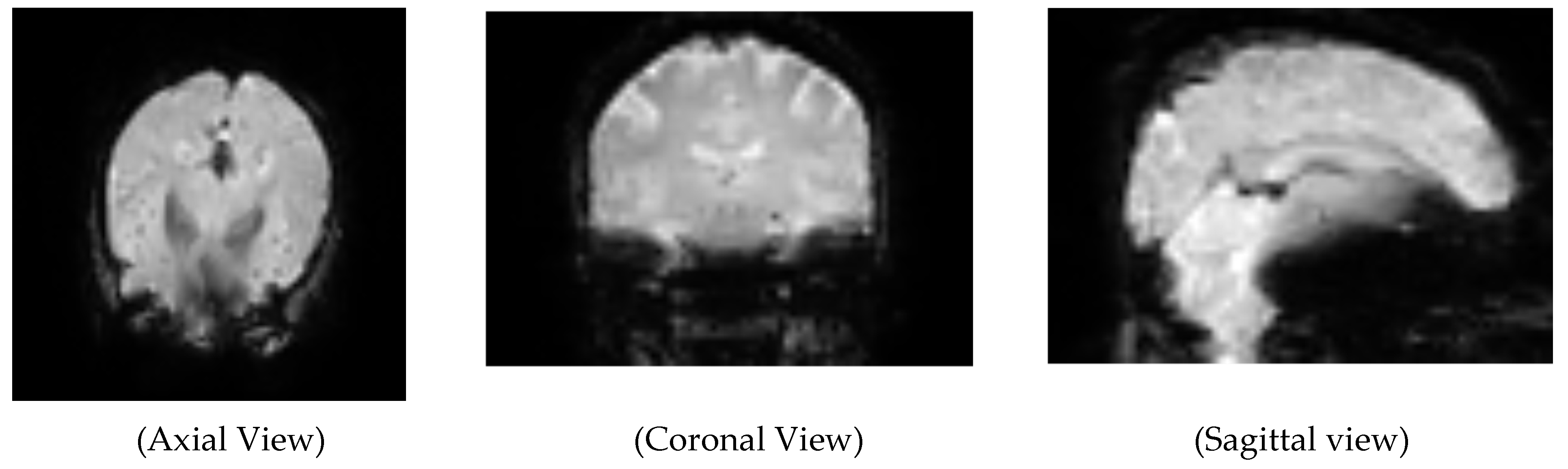
The dataset was collected from the ADNI, which is a well-known longitudinal study (https://adni.loni.usc.edu/, accessed on 13 February 2024). The data were downloaded based on a Philips scanner with an EPI of 140 scans per volume, and the field strength was set to 3.0. The TE and TR were 30.001 and 3000.0, respectively; the flip angle was 80.0, and the number of slices was 6720.0, with a slice thickness of 3.313. All scans were originally downloaded in DICOM format. A total of 204 subjects’ data were obtained for detailed experimentation. Details for the data are provided in

Table 2. Details about rs-fMRI data from ADNI.

Stage	Number of Subjects	fMRI Scans
CN	50	182
SMC	23	36
EMCI	54	213
LMCI	33	145
MCI	6	14
AD	33	116

. An unprocessed version of the rs-fMRI scan of an MCI subject is shown in Figure 3. The metadata for the same patients for this study were collected, including subject characteristics that included their demographics, family history, medical history, and clinical assessment, including MoCA.

3.2. Preprocessing Techniques for the rs-fMRI Dataset

The rs-fMRI dataset was preprocessed using typical techniques that were employed in prior studies [32,34,35]. The ADNI database provides the data in DICOM format, and the dicom2nifti library was used to convert the data to a NIFTI format. This study’s preprocessing techniques included temporal filtering, slice timing, head motion correction, removal of unnecessary frames, normalization, smoothing, regressing nuisance factors, and skull stripping. Preprocessing techniques were applied to rs-fMRI data using various Python-based packages, including ANtspyNET 0.0.1, simple-ITK 2.4.0, Nilearn 0.10.4, and Nipype 1.8.6.

The first ten and last six fMRI frames were eliminated during preprocessing as they contained no critical information. The correction technique for slice time was then applied to ensure that the acquired time of slices adhered to a repetition time. Nipype was used for this purpose so that a set of instructions could be written for the slice timing correction. The middle slice was used as the reference point, and the workflow ran the slice timing correction steps and output the corrected data. Subsequently, the impacts of the patient’s skull motion at the time of data gathering were eliminated using realignment and head motion correction. The motion correction technique was used to calculate and correct this motion by choosing a template image from the fMRI dataset and applying registration to all subsequent images in the series to this reference.

Skull stripping or brain extraction was the next stage of preprocessing. This step involved eliminating non-brain tissues from the brain scans, which required determining the spherical radius, the brain’s gravity center, and the intensity histogram. Subsequently, image registration was carried out to ensure that the spatial domain of each brain scan was the same. AntspyNet was used for brain extraction, with a threshold value set to 0.5 for mapping the probability brain mask to the original image.

Let $X\in {\mathbb{R}}^{H\times W\times D}$ represent the input MRI image, where $H, W, \mathrm{a}\mathrm{n}\mathrm{d} D$ are the height, width, and depth of the 3D image, respectively. Let a model for skull stripping be represented as $Y=\mathcal{M}(X,\theta )$ where $\theta$ are parameters of the model. Then, $Y(i,j,k)$represents the probability that voxel $(i,j,k)$belongs to brain tissue where $Y\in {\mathbb{R}}^{H\times W\times D}$. The binary mask of the brain is generated when performing skull stripping with a threshold of 0.5, as given in Equation (1):

$$M\left(i,j,k\right)=f\left(x\right)=\left\{\begin{array}{c}1, if Y\left(i,j,k\right)\ge 0.5\\ 0, if Y\left(i,j,k\right)<0.5 \end{array}\right.$$

(1)

Hence, the skull-stripped brain image $X_{brain}$ was obtained by element-wise multiplication of the original MRI image $X$ with the brain mask $M$, as given in Equation (2):

$$X_{brain}=X \odot M$$

(2)

Then, spatial smoothing was employed to reduce the noise without influencing the fMRI scan’s activated region. Using a 4 mm full width at half maximum kernel, deconvolution was performed on 3D pictures with a cubic Gaussian filter to achieve spatial smoothing. The next stage involved eliminating the noise in the fMRI caused by physiological artifacts. In this step, the data were regressed, and six motion parameters, white lesions, and global mean signals were eliminated. Lastly, low- and high-level noise resulting from psychological aberrations—such as breath, pulse, or scanner movement—was removed from the fMRI data using a bandpass filter (0.01 Hz–0.08 Hz). 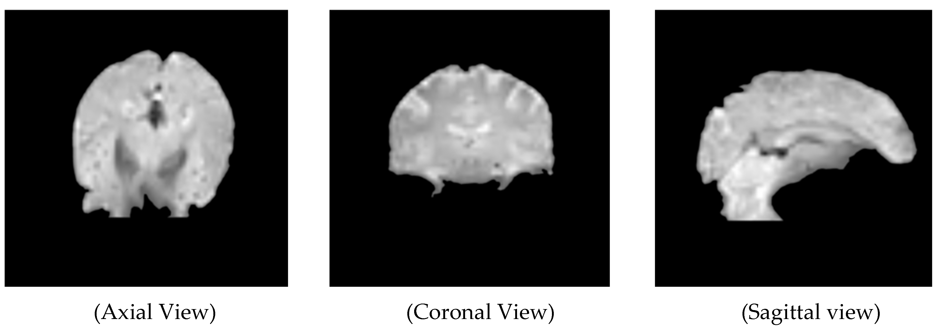Figure 4 represents an rs-fMRI scan of an EMCI patient after the deletion of extra frames and the application of slice time correction, realignment, skull movement correction, brain extraction, and normalization.

3.3. Functional Connectivity of the Brain Networks

There were 130 time points in the analyzed fMRI data at this stage. The ROIs were located using a brain atlas that included 90 areas. An automated anatomical labeling brain atlas [36] was utilized for this task. Each time series inside a brain ROI was averaged to determine the ROI’s time series. A matrix of 90 × 130 was produced for each rs-fMRI scan, and 90 ROIs were calculated by combining the average of each time-series value of the relevant region.

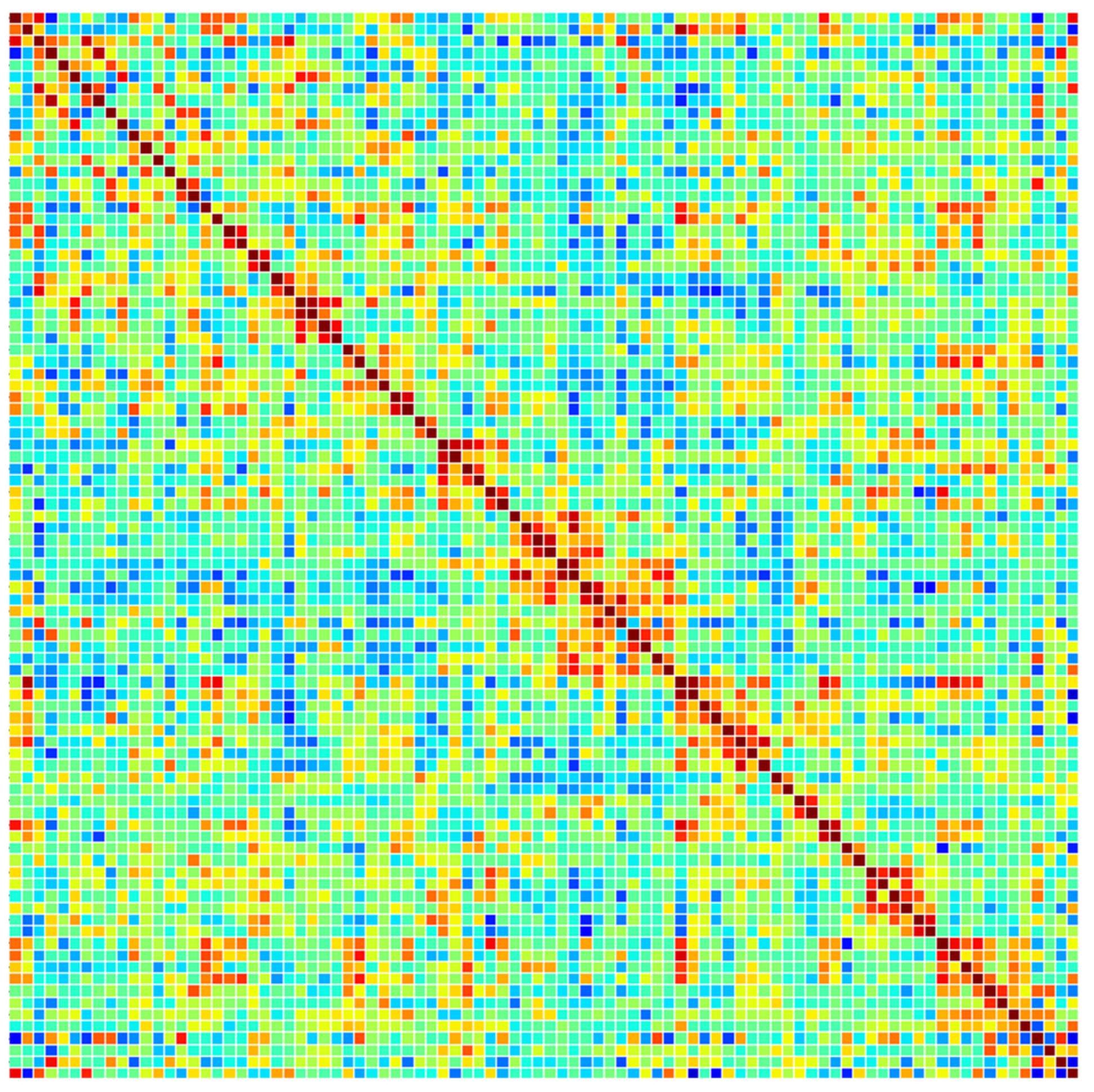
A typical method for determining a linear connection is to utilize Pearson’s correlation coefficient (PCC). It was used to calculate the functional connectivity of the brain ROI after computing a 90-ROI time series from preprocessed rs-fMRI data. Let X and Y be the rows and columns of the time-series matrix of 90 ROI; then, PCC can be determined as given in Equation (3):

$$r={\displaystyle \frac{\sum _{i=1}^N(X_i-\overline{X})(Y_i-\overline{Y})}{\sqrt{{(X_i-\overline{X})}^2}\sqrt{{(Y_i-\overline{Y})}^2}}}$$

(3)

where $\overline{X} \mathrm{a}\mathrm{n}\mathrm{d} \overline{Y}$are the means of $X$ and $Y$, respectively. Hence, a brain network was represented by the 90 × 90 data matrix that was produced. Each cell ($i$th row and $j$th column) in this symmetric matrix indicated the connection between the i-th and j-th brain regions. The values on the main diagonal indicate the total connectivity throughout the brain region, whereas the values on the upper and lower triangular matrices contain information on the strength of connectivity between different brain regions. Only the upper triangular matrix (4005 = 90 × 80/2) was used as the model’s input, as the upper and lower triangular matrices reflect the same information. To train the deep learning network on a sizable dataset and enable it to learn a variety of features, additional data were created by applying augmentation to the functional connectivity (correlation coefficients) dataset. Data augmentation renders a trained model more reliable and accurate. Forty-five ROIs were created randomly from a sample of participants, and the corresponding rows and columns of the original data were replaced to create the augmented dataset. Figure 5 displays a functional connectivity matrix of a preprocessed rs-fMRI scan of an MCI patient based on Pearson correlations.

For instance, the fifth row and fifth column of the original correlation matrix would be changed to the fifth row and fifth column of subject number 13 if a randomly picked ROI was 7 and the subject number was 13. This data augmentation technique was inspired by J. Regina et al. [37]. A graphical representation of rs-fMRI preprocessing is illustrated in Figure 6. After preprocessing, a balance dataset for functional connectivity matrices was created. The numbers of samples in each class appear in

Table 3. Connectivity matrices created after preprocessing rs-fMRI data.

Stage	Number of Connectivity Matrices
CN	495
SMC	354
EMCI	575
LMCI	399
MCI	305
AD	318

.

3.4. Preprocessing of Subject Characteristics and Clinical Data

First, the data were merged into a single CSV file to preprocess the dataset. These files were merged based on the participant ID that was common to each file. The final CSV file included seven variables on demographics, 20 variables on family history, 34 variables on medical history, and 1 variable from the MoCA assessment (final MoCA score). Hence, a total of 62 variables were in the file that was used as input for the model. All categorical variables, such as marital status and parents’ or siblings’ AD histories, were one-hot encoded. The continuous variables, such as MoCA scores, were subjected to normalization. This technique transforms each value to a range, typically [0, 1], based on the minimum and maximum values in the data. For a value $x$, the scaled output $x_s$ is given in Equation (4):

$$x_s={\displaystyle \frac{x-x_{min}}{x_{max}-x_{min}}}$$

(4)

3.5. Convolutional Neural Network

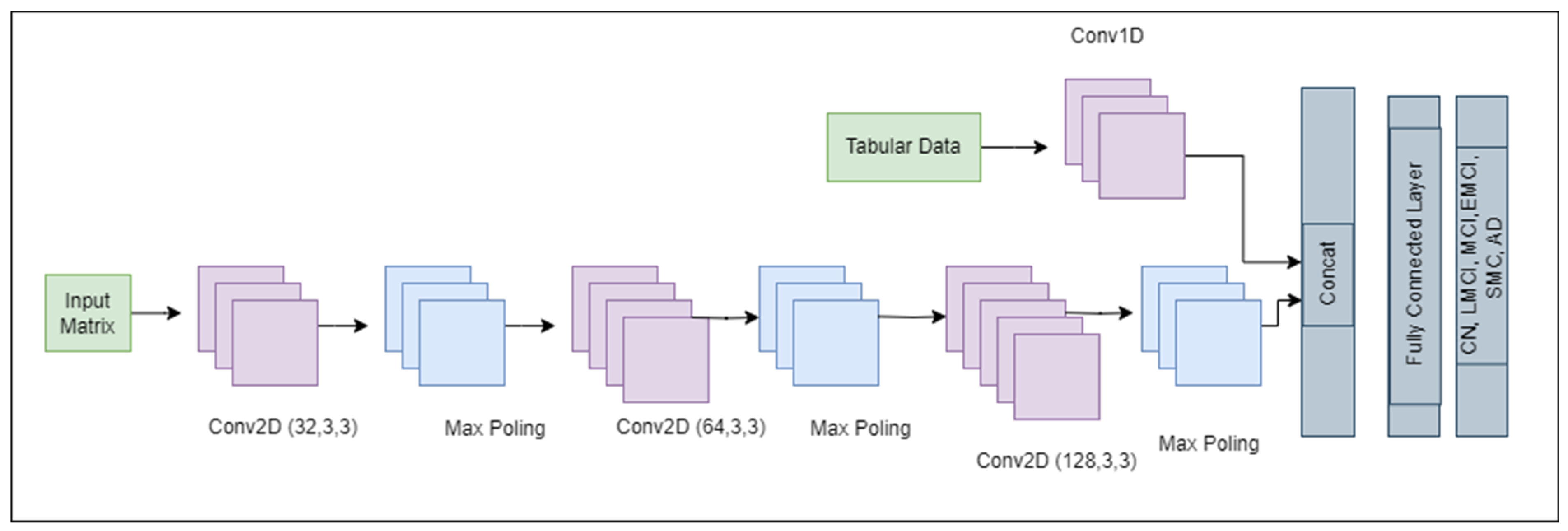
CNNs are a key component of computer vision and are utilized in many domains, including natural language processing, autonomous driving, medical image analysis, and image and video recognition. In this paper, a simple CNN was used, as shown in Figure 7. The model began with a convolutional layer (Conv2D) with 32 filters, which captured low-level features such as edges. The output of the Conv2D layer with 32 filters was a stack of 32 feature maps, 1 for each filter, as represented in Equation (5).

$$O_k\left(i,j\right)={\sum }_{m=0}^{M-1}{\sum }_{n=0}^{N-1}I\left(i+m,j+n\right).K_k\left(m,n\right)+b_k, for k=\mathrm{1,2},\dots , 32$$

(5)

where $O_k$is the output feature map for the k-th filter, $I$ is used for the input image, $K_k$ is the k-th convolutional kernel, $b_k$ is the bias term for the k-th filter, and k is the filter index (ranging from 1 to 32 for the 32 filters). A max pooling layer lowers the spatial dimensions of the previous layer, thereby focusing on the most prominent features. The output matrix of the max pooling layer was calculated from Equation (6):

$$P\left(i,j\right)=\underset{m,\mathit{n}}{\max }{O}_k(i,+m, j+n)$$

(6)

where $P\left(i,j\right)$ is the pooled output. This pattern was repeated with greater numbers of filters (64 and 128) in subsequent convolutional layers, allowing the model to learn more complex patterns. The output from the convolutional layers was compressed into a 1D vector and was then run through a dense layer having 128 neurons to integrate the features into a comprehensive representation. To avoid overfitting, a dropout layer was incorporated; this layer randomly deactivates a subset of the neurons during training. For the tabular data represented as $X$, 1D Conv was used to extract features using Equation (7), which is a slight modification of Equation (5).

$$O_i={\sum }_{j=1}^{k}X\left(i+j-1\right)\times Kernel\left(j\right)+Bias$$

(7)

The outputs from Equations (5) and (7) were concatenated. Finally, the output layer, which is a dense layer with six neurons corresponding to the number of classes in the classification task, was applied. This architecture possessed a total of 1,420,678 trainable parameters. It leverages the strengths of convolutions for feature extraction and dense layers for classification to provide a robust framework for image recognition tasks.

3.6. Transformer

Originally, transformers were designed for natural language processing (NLP) projects, but they have also been employed for image classification. They can capture long-range sequences and can thus be used to manage graph-based data too. Although the connectivity matrices are not real graphs, the nature of the data is the same. Transformers use a self-attention mechanism that detects the pertinent segment of sequences needed to complete the given task. These models are also suited for capturing the contextual information that is not possible to capture in CNN. Equation (8) provides a scale dot product that can be used to calculate the value of the primary attention mechanism:

$$Attention\left(K,Q,V\right)=A(Q,K) V$$

(8)

where K, Q, and V denote the key, query, and value, respectively. An attention function is often defined as follows: it maps a set of key-value pairs {k,v} and a query q to an output o. The scaled dot product for attention values is calculated from Equation (9):

$$A\left(Q,K\right)=softmax\left({\displaystyle \frac{Q{K}^T}{\sqrt{d_{att}}}}\right)$$

(9)

where $d_{att}$ corresponds to queries and keys’ dimensions. Transformers specifically employ a multi-head attention mechanism, which has the mathematical expressions given in Equations (10) and (11).

$$MultiHead\left(Q,K,V\right)=\left[{Head}_1, \dots , {Head}_n\right]W_o$$

(10)

$${Head}_i=(Q{W}_i, K{W}_i, V{W}_i)$$

(11)

where $W$ denotes all the learnable parameter matrices.

The encoder–decoder-based transformer model uses positional encoding to map input into a higher-dimensional space, then a multi-headed attention layer, followed by normalization and finally the fully connected layers. The formula for positional encoding at position $i$ and dimension $j$ is presented in Equation (12):

$$PE\left(i,j\right)=\left\{\begin{array}{c}\mathit{sin}\left({\displaystyle \frac{i}{{\mathrm{10,000}}^{2j/d_{model}}}}\right) if j is even\\ \mathit{cos}\left({\displaystyle \frac{i}{{\mathrm{10,000}}^{2j/d_{model}}}}\right) if j is odd\end{array}\right.$$

(12)

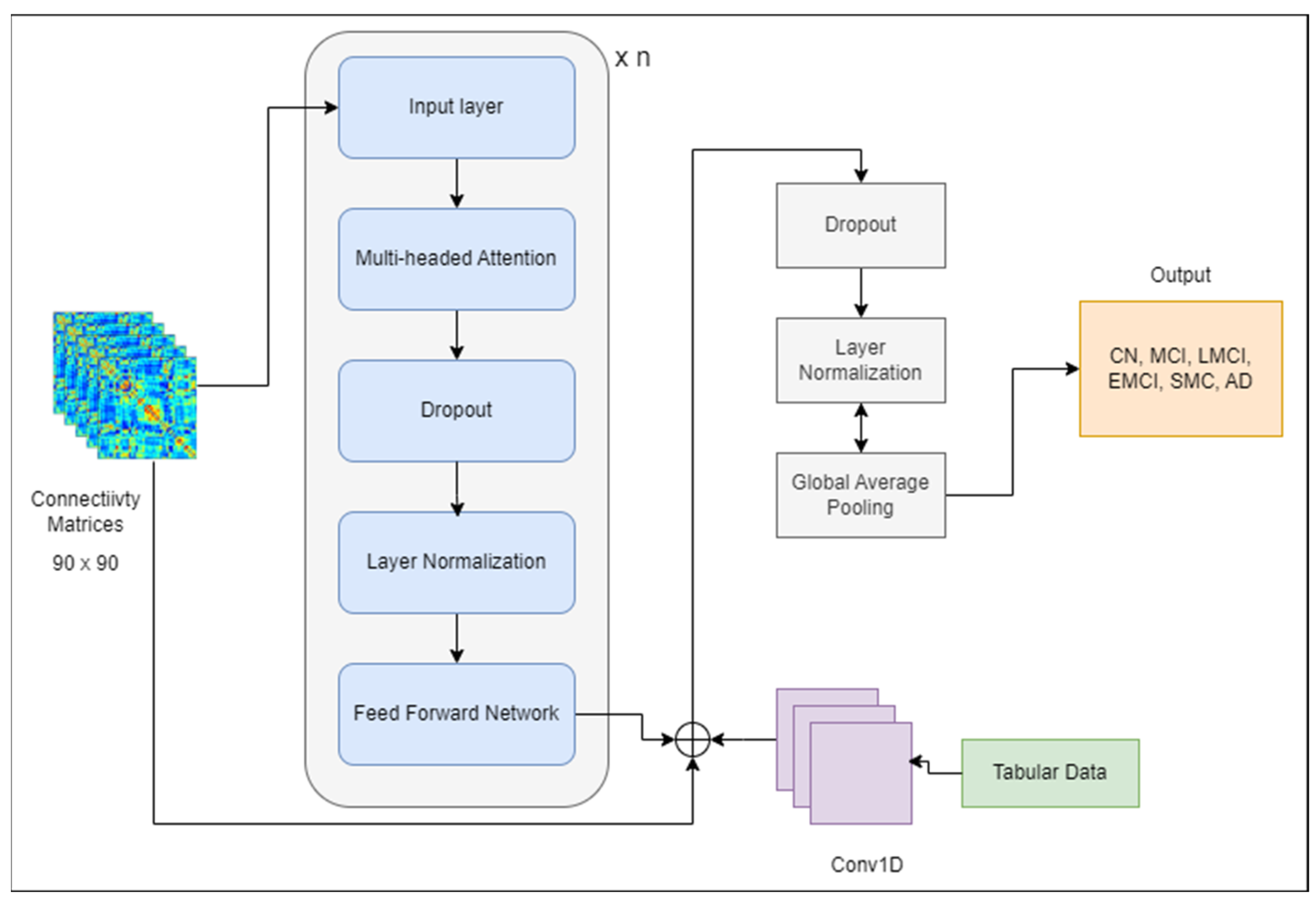
where $PE\left(i,j\right)$ is the positional encoding at position $i$ and dimension $j$, and the $d_{model}$ term is the dimension of the model. The encoded representation obtained from the transformer encoder is passed as input to the decoding part, which generates output. However, only the encoder is used for classification purposes. A simple model was developed, shown in Figure 8, that used a transformer block leveraging multi-head attention and feed-forward neural networks. The output of tabular data from Equation (7) was concatenated with the output of the transformer model to pass to the next layers. Dropout and layer normalization were applied to improve the model’s generalization and stability during training. Adam was employed as an optimizer, and sparse categorical cross-entropy was utilized for the loss function.

3.7. Hybrid Transformer-CNN Model

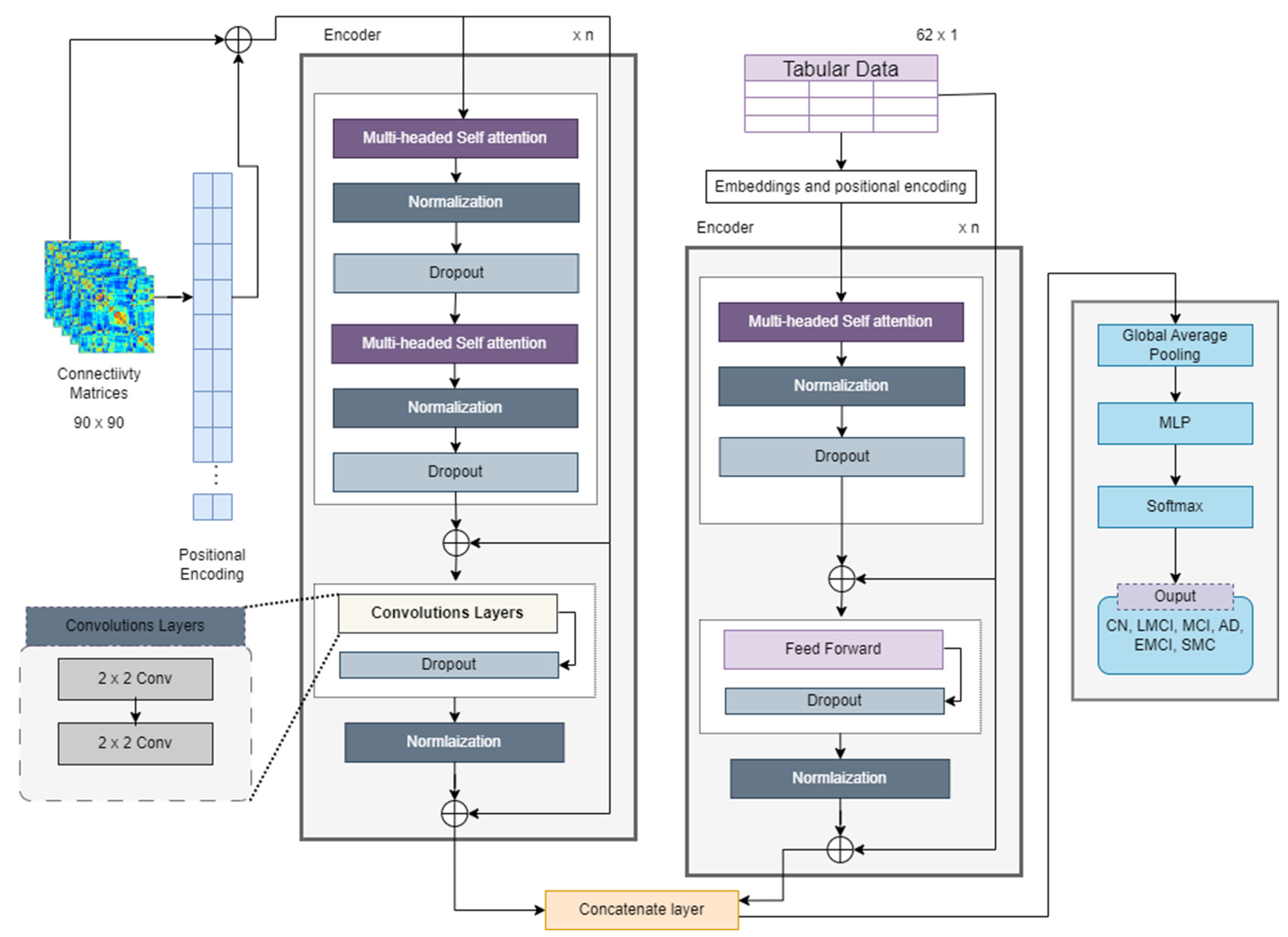
The proposed hybrid model employs the transformer model by A. Vaswani et al. [13]. Figure 9 illustrates the novel model’s architecture. Transformers are capable of handling raw input data, in the form of tokens, and they internally learn embeddings during their training process. For NLP datasets, words must be converted into embeddings, which means the connectivity matrix can be directly input into the model. The connectivity matrix itself can serve as a meaningful input representation for a transformer model. Each entry in the matrix represents the strength or presence of a connection between two entities (nodes, features, etc.). In such a case, each cell or entry in the connectivity matrix can be treated as a token for the transformer model.

• Positional Encoding

The connectivity matrix was preprocessed with normalization and scaling before feeding it into the transformer model. Since transformers do not inherently understand the order of tokens in a sequence, positional encoding is crucial for preserving the sequence information. Positional encoding is typically computed using sinusoidal functions. Such encoding tells the model the order of tokens in the input sequence, which is crucial for remembering the sequences of nodes and edges of matrix data. By adding unique positional information to each token’s embedding, positional encoding ensures that the model distinguishes tokens with the same semantic meaning but different positions. The dense interpolation module was not implemented because there was no need for that. The positional encodings for fMRI data that are represented as $X \in {\mathbb{R}}^{90\times 90}$ are given in Equations (13) and (14). For the connectivity matrix, the positional encoding formula was expanded to include interaction terms between the row and column indices $i$ and $j$.

$$PE\left(i,j,2k\right)=\sin \left({\displaystyle \frac{i.j}{{10000}^{\frac{2k}{d}}}}+{\displaystyle \frac{i+j}{{10000}^{\frac{k}{d}}}}\right)+\alpha \sin \left({\displaystyle \frac{i^2+j^2}{{10000}^{\frac{2k}{d}}}}\right)$$

(13)

$$PE\left(i,j,2k+1\right)=\cos \left({\displaystyle \frac{i.j}{{10000}^{\frac{2k}{d}}}}+{\displaystyle \frac{i-j}{{10000}^{\frac{k}{d}}}}\right)+\beta \cos \left({\displaystyle \frac{i^2-j^2}{{10000}^{\frac{2k}{d}}}}\right)$$

(14)

where $i$ and $j$ are the row and column indices, respectively; $d$ is the total dimension of the embedding space; $k$ is the index of the embedding dimension; and $\alpha$ and $\beta$ are constants that can be tuned as hyperparameters to control the influence of the additional nonlinear terms. The encodings for tabular data$T \in {\mathbb{R}}^{62\times 1}$ are calculated using Equation (12).

• Combination of Transformer and CNN

For the input matrix, positional encoding was first generated and was then combined with positional encoding properties. The information was sent to an attention-based block that included a multi-headed attention mechanism with convolutional layers. The proposed model was named as the Transformer_CNN (see Figure 9), because 2D CNN layers are applied instead of the feed-forward network calculated according to Equation (5). Multi-head self-attention (MHA) captures global dependencies between the input features, as given in Equation (10). The CNN-based feed-forward network extracts local patterns and refines the features. Simply put, the output from MHA is passed forward to the CNN network. This process means the encoder of the transformer-based model can be represented as shown in Equation (15).

$$O_x={Conv2D(MultiHead\left(Q,K,V\right)+PE)=X}_k\left(i,j\right)\left(Multiheaded\left(Q,K,V\right)+PE \left(X_{ij}\right)\right)$$

(15)

where ${ X}_k\left(i,j\right)$ represents the convolution matrix.

• Multimodal Feature Fusion

For tabular data, the transformer encoder consists of self-attention, normalization dropout, and feed-forward layers. The output from these layers is represented as $O_t$. Both outputs are then concatenated; however, the interaction between two modalities is calculated first, as given in Equation (16) below. This step ensures that connectivity features and clinical features are jointly optimized rather than merely being concatenated.

$$X_{interacted }=ReLU(\left(O_x{W}_1\right).(O_t{W}_2\left)\right)$$

(16)

This interaction layer takes the processed connectivity and tabular data, applies matrix transformations, and generates the interacted feature tensor $X_{interacted }$. The final concatenation of both data types is given in Equation (17). The fusion is performed using a weighted combination of direct concatenation and interacted features.

$$O_{concat}=\lambda \left(O_x\oplus O_t\right)+\left(1-\lambda \right).X_{interacted }$$

(17)

where $\lambda$ is the scaling factor that is used for the weighted combination of the output tensors and the interaction tensor. The CNN efficiently extracts the local connectivity features from brain networks, whereas the transformer adds further understanding by capturing global interactions among the clinical features. The interaction mechanism ensures a joint learning process, leading to better multiclass classification accuracy for AD staging. Instead of treating these modalities separately, the proposed approach allows their interaction at an earlier stage, which enriches the feature space and improves the classification accuracy.

• Classification

The final matrix after fusion is eventually fed into a multi-layer perceptron (MLP) model, which passes the final features to a SoftMax layer of classification. After encoding, the features again pass through an MLP with a SoftMax layer for classification. For an MLP with L layers, the transformation at each layer $l$ can be written as in Equation (18):

$$h^{\left(l\right)}=\sigma (T{W}^{\left(l\right)}{h}^{\left(l-1\right)}+b^{\left(l\right)})$$

(18)

The SoftMax function converts the raw scores or logits obtained from MLP into probabilities, as per Equation (19). An algorithmic representation of the complete flow of architecture appears in Algorithm 1.

$${softmax\left(z\right)}_i={\displaystyle \frac{\mathrm{e}\mathrm{x}\mathrm{p}\left(z_i\right)}{{\sum }_{j=1}^{k}exp\left(z_j\right)}},$$

(19)

where

• $z_i$is the i-th element of the input vector z.
• $\exp \left(x\right)$denotes the exponential function.
• ${\sum }_{j=1}^{k}exp\left(z_j\right)$represents the sum of the exponentials of all elements in the input vector z.

Algorithm 1: Algorithm for hybrid Transformer Model

Input: Connectivity matrices of rs-fMRI data [],                           <- Connectivity matrices in .mat format        Tabular_data []                                        <- Tabular matrices in .csv format    Output: final_output                                            <- Final label of classification 1.  function Hybrid_Transformer (Connectivity_matrices []) 2.  3.    convolutional_layers = n 4.    for (each Connectivity_matrix in Connectivity_matrices []) do 5.      encodings = positional_encoding(Connectivity_matrix) 6.      attention_matrix = Multi_headed_attention(encodings, head_size, num_heads, n_blocks, attention_dropout) 7.      normalized_tensor = Normalization(attention_matrix) 8.      tensor_d1 = dropout(normalized_tensor) 9.         attention_matrix = Multi_headed_attention(tensor_d1) 10.       normalized_tensor1 = Normalization(attention_matrix) 11.       tensor_d2 = dropout(normalized_tensor1) 12.       concatenated_tensor = concat(Connectivity_matrix, tensor_d) 13.       for (i in range (convolutional_layers)) do 14.        feed_forward_tensor = conv2D (concatenated_tensor, ff_dim, n_kernel) 15.       END For 16.       for (each Tabular_data_matrix in Tabular_data []) do 17.       encodings = positional_encoding(Tabular_data_matrix) 18.       tabular_tensor = Multi_headed_attention(encodings, head_size, num_heads, n_blocks, attention_dropout) 19.       normalized_tensor = dropout (Normalization(tabular_tensor)) 20.       tabular_tensor = concat (normalized_tensor, Tabular_data_matrix) 21.       END For 22.       conacte_multimodal = conact(feed_forward_tensor, tabular_tensor) 23.       tensor_d3 = dropout(conacte_multimodal) 24.       normalized_tensor2 = Normalization(tensor_d3) 25.       global_pooling_tensor = Global_Average_pooling(normalized_tensor2) 26.       MLP_output = Multi_Layer_Perceptron(global_pooling_tensor, n_hidden_layers, n_hidden_neurons, mlp_dropout, mlp_activation) 27.       final_output = Softmax_layer (MLP_output) 28.  End for 29.  return final_output 30. End Hybrid_Transformer

3.8. Ablation Study Design

To assess the contribution of each component in the proposed hybrid model, ablation experiments were conducted by systematically removing or isolating specific components and evaluating their performance:

• CNN-only Model: This variant replaces the Transformer module with a fully CNN-based architecture to assess the impact of local feature extraction.
• Transformer-only Model: This version removes CNNs and relies solely on transformer-based feature extraction.
• Hybrid Model Without Multimodal Fusion: This setup evaluates the impact of integrating clinical data by training on rs-fMRI features only.
• Proposed Hybrid Model: Full architecture with CNNs for local feature extraction, transformers for global context, and multimodal fusion of rs-fMRI and clinical data.

3.9. Experimental Setup

To estimate the outcome efficiency of the proposed network, a functional connectivity matrix dataset was employed with a dimensionality of 90 × 90, which corresponds to the pairwise correlations between 90 predefined brain regions of interest (ROIs). This representation effectively captures inter-regional neural communication, which is known to be disrupted in various stages of Alzheimer’s disease (AD). Two classification tasks were conducted: (i) a binary classification (AD vs. non-AD) to support early diagnosis, and (ii) a multiclass classification across six clinically defined stages (CN, SMC, EMCI, MCI, LMCI, and AD) to reflect the progressive nature of the disease.

The model was implemented using the PyTorch v2.4.0 framework and trained on an NVIDIA Tesla K80 GPU with 12 GB RAM. A 70:30 train–test split was employed initially to allow sufficient data for both training and evaluation. To ensure robustness and minimize overfitting on small datasets, 5-fold cross-validation was incorporated. This provided a comprehensive performance assessment across multiple subsets, enhancing generalizability. Each batch contained 32 samples, and training was conducted for 50 epochs using the Adam optimizer with a learning rate of 0.001. The model was evaluated using standard classification metrics, accuracy, recall, precision, and F1-score to provide a balanced view of performance, especially in the presence of potential class imbalance.

All experiments, including those for baseline models, were conducted under identical conditions to ensure a fair comparison. The same preprocessing pipeline was employed on the ANDI dataset and train–test splits for each architecture. This consistent experimental protocol strengthens the validity of the comparative analysis, enabling a clear assessment of the hybrid model’s benefits.

4. Results and Discussion

In this section, the results of the experiments performed with state-of-the-art models on the ADNI dataset are explained.

4.1. Benchmark Networks

For benchmark comparison, nine different networks were compared with the proposed network, as shown in

Table 4. Results from benchmark networks and the proposed hybrid transformer mode model for six-class classification.

Classification Task	Model	Accuracy (%)	Precision (%)	Recall (%)	F1-Score (%)	No. of Parameters
6-class (CN, AD, MCI, LMCI, EMCI, SMC)	CNN	80	79	80	79	2.05 million
	EfficientNet-B0	95.26	95.12	95.09	95.1	4.015 million
	MobileNet-v2	94.66	93.99	94.05	94.02	3.4 million
	ShuffleNet-v2	90.25	90.12	90.19	90.15	1.4 million
	RegNet	95.77	95.56	95.24	95.40	10.6 million
	ConvNext	95.82	95.76	95.77	95.76	28 million
	Transformer	78.29	78.24	78.14	78.19	24 million
	Swin Transformer	95.35	94.00	94.25	94.12	27.501 million
	MRI_ViT with attention-embedded 1D CNN	95.02	94.77	94.78	94.76	21.83 million
	Hybrid_transformer	96	96.09	96.12	96.10	0.879 million

.

• Convolution Neural Network

A CNN model with three convolutional layers to extract and downsample features was trained on the data. Every convolutional layer was followed by a max pooling layer; then, after flattening the output, a dense layer with dropout for regularization was used before the final SoftMax layer to classify the input into one of six categories. Sparse categorical cross-entropy loss was employed in the model. The hyperparameters used during training were a batch size of 32 and the optimizer Adam with a learning rate of 0.001. In addition, a different validation dataset was utilized to assess the model’s performance. During training, the model showed significant improvements in both its training and validation performance. Initially, the model achieved a training accuracy of 60% and a validation accuracy of 71.6%, with losses of 1.1019 and 0.6965, respectively. By epoch 4, the losses had decreased to 0.4552 and 0.5922, whereas the training accuracy had increased to 82.78%, and the validation accuracy had increased to 75.71%. By the end of training, the model achieved a training accuracy of 96%. However, the validation accuracy was only 80%, which indicates room for improvement.

2.

Transformer

The architecture of the transformer-based model started with a custom transformer block that was designed to handle sequence data. This block contained an MHA mechanism that enabled the model to highlight important parts of the input sequence. A feed-forward network with dense layers and ReLU activation to detect the complex patterns of data was used. After normalization, dropout layers were employed to add stability to the training. After the transformer block, global average pooling layers were used to lower the dimensionality, and a final dense layer with a SoftMax activation returned the class probabilities. The training logs for the transformer-based model indicate moderate performance improvements over 10 epochs. Initially, the model achieved a training accuracy of 67.6% and a validation accuracy of 72.35%, with losses of 0.9403 and 0.7103, respectively. Staying on this path, by the final epoch the model had attained a training accuracy of 93.46% and a validation accuracy of 78.29%.

3.

EfficientNet

The EfficientNet architecture was proposed by Google AI [38]. A modified version of EfficientNet-B0, adapted for single-channel input images and specifically designed to address the unique characteristics of the preprocessed fMRI dataset, was used as a benchmark in the current study. Additionally, the use of more advanced architecture was explored. EfficientNet was applied for its unique scaling method, which balances network depth, width, and resolution to improve both performance and efficiency. The pretrained EfficientNet-B0 model was modified to process 90 × 90 single-channel input matrices by altering the initial convolutional layer and adjusting the final classifier layer to accommodate six output categories. The model was trained with dropout for regularization and showed an effective classification performance on the task. The modified version of EfficientNet achieved an accuracy of 95.26%, precision of 95.12%, recall of 95.09%, and F1-score of 95.1%. The network had a total of 4.105 million parameters.

4.

MobileNet-V2

MobileNetV2 [39] is a lightweight CNN model that has been pretrained on the ImageNet dataset. The main reason to adopt this model is its lightweight design, which is derived from depth-wise separable convolutions. The model comprises two modules, each consisting of three layers. These modules start and end with 1×1 convolutional layers, which are the first step in the depth-wise separable convolution; the second layer consists of a convolutional layer that combines the operation of the first layer in a depth-wise manner. The activation function ReLU is applied in each layer. The model was modified to process 90 × 90 single-channel input matrices by altering the initial convolutional layer and adjusting the final classifier layer for six output categories. It achieved an accuracy of 94.66%, with a total of 3.4 million parameters in the network.

5.

ShuffleNet-v2

ShuffleNetV2 [40] is a lightweight CNN network designed for high efficiency in mobile and edge devices. It improves upon the original ShuffleNet by optimizing the memory access cost and reducing the computational overhead. The architecture features channel shuffling and group convolution to enhance the information flow while maintaining low complexity. Additionally, it incorporates pointwise group convolutions and depth-wise separable convolutions, significantly reducing the number of parameters and FLOPs. ShuffleNetV2 is known for its trade-off between speed and accuracy. It outperforms many lightweight models, such as MobileNetV2, in inference efficiency, while maintaining its accuracy, which makes it a sound choice for resource-constrained environments. The total number of parameters for this network is 1.4 million. The model obtained an accuracy of 90.25%, precision of 90.12%, recall of 90.09%, and F1-score of 95.1%.

6.

Swin Transformer

Swin transformer [41] is a vision transformer-based model that is employed to leverage its cutting-edge hierarchical structure and window-based attention mechanism, which shifts from the convolutional paradigm to transformers for visual tasks. Swin transformer operates by dividing the input into non-overlapping windows and applying self-attention within each window; this step is followed by shifting the windows to capture the interactions across various regions of the image. The mechanism allows the Swin transformer to capture both local and global dependencies in the data effectively. In this case, the 90 × 90 single-channel matrices were processed in a hierarchical manner, enabling the model to learn fine-grained features while also considering the broader context. The shifted window approach further enhanced the performance by allowing the model to maintain a balance between computational efficiency and representational power. Swin transformer’s use of MHA at different spatial scales made it particularly suited for managing neuroimaging data, where capturing subtle patterns across different regions of the input is essential. The model achieved an accuracy, precision, recall, and F1-score of 95.35%, 94%, 94.24%, and 95.12%, respectively, with 27.501 million parameters.

7.

RegNet

RegNet [42], a family of network designs that focuses on efficiency and scalability, was incorporated in this study. RegNet’s design emphasizes regularizing a model’s width and stage depth, which enabled us to fine-tune the architecture for the ADNI dataset. The regularization of the network width (the number of channels in each block) allowed us to achieve balanced model complexity without overfitting. The stage-wise design of RegNet, with repeated bottleneck-like structures, enabled the model to process data efficiently while maintaining its strong learning performance. This characteristic is particularly helpful when working with data like neuroimaging matrices, where balancing the computational cost with accuracy is crucial. RegNet provides the advantage of being adaptable to different scales of datasets, which renders it a strong contender for training large-scale, multiclass classification models. The application of RegNet in the proposed study demonstrated robust performance, with the efficient extraction of both local and global features from the 90 × 90 input matrices while maintaining computational efficiency. The results included accuracy, precision, recall, and F1-score of 95.77%, 95.56%, 95.24%, and 95.40%, respectively, from the RegNet architecture. The total number of parameters was around 10.6 million.

8.

ConvNeXt

ConvNeXt was employed as a benchmark. This model is another modern CNN architecture; it was introduced by Facebook AI Research and was inspired by vision transformers [43]. ConvNeXt incorporates depth-wise convolutions, layer normalization, and a ResNet-style structure; it also includes updates that align with modern deep learning practices. In this setup, ConvNeXt processed 90 × 90 single-channel matrices, passing through layers that captured both fine-grained and global features. The model showed strong generalization capacity due to its deep architecture and regularization techniques, such as dropout. The results for accuracy, precision, recall, and F1-score were 95.82%, 95.76%, 95.77%, and 95.76%, respectively, using ConvNeXt architecture with about 28 million parameters.

9.

MRI_ViT with attention-embedded 1D CNN

This approach is a multimodal data fusion technique for classifying different stages of AD. The method combined a vision transformer and 1D CNN multimodal analysis of MRI and clinical data. For clinical data, an enhanced squeeze-and-excitation block was introduced that was responsible for extracting features relevant to MRI data. Accuracy, precision, recall, and F1-score of 95.02%, 94.77%, 94.78%, and 94.76%, respectively, were achieved using this architecture with about 21.83 million parameters.

4.2. Hybrid Transformer-CNN Model

4.2.1. Experimental Results for Multiclass Classification

After extensive experiments with various models, the hybrid transformer model for different hyperparameters was tested. The results of the standalone CNN and transformer were inadequate, so a hybrid model that integrated the strengths of both models to efficiently capture and process spatial and sequential patterns in the data was developed. The model begins with an input layer of shape (90, 90). The input layer is then introduced to multiple transformer encoder blocks. Each block comprises two multi-head attention layers with residual connections and layer normalization. These layers are followed by convolutional layers to enhance the feature extraction; these blocks aim to capture dependencies in the sequence data.

To make the data suitable for further processing, a global average pooling layer is used to reduce the dimensionality of the encoded sequences. The output of this layer is fed to the MLP, which is a combination of multiple dense layers, each followed by a dropout layer. The final dense layer employs SoftMax activation to produce the classification output. This hybrid model achieved an accuracy of 96% for multiclass classification. The loss and accuracy curves for training and testing using five-fold cross-validation are presented in Figure 10.

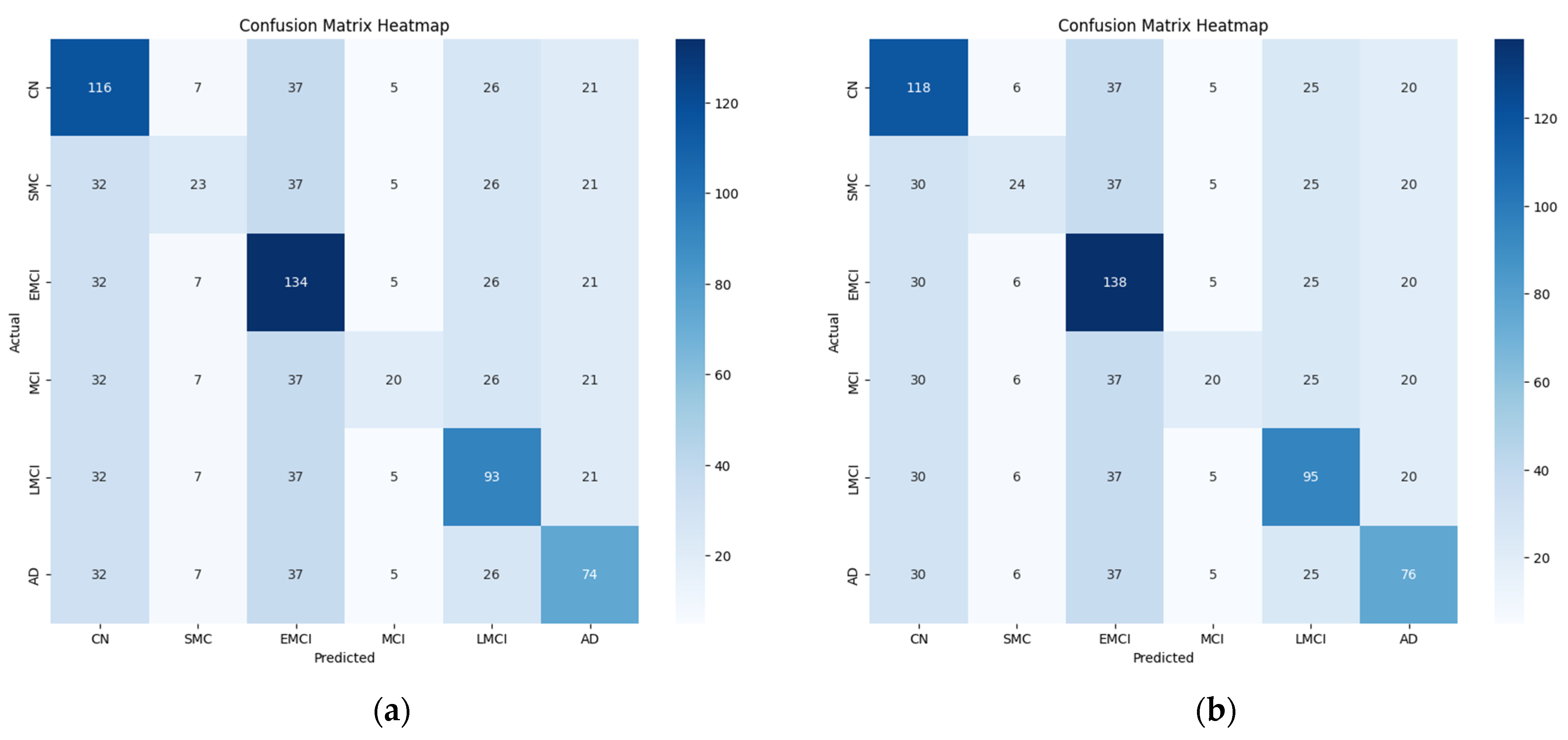
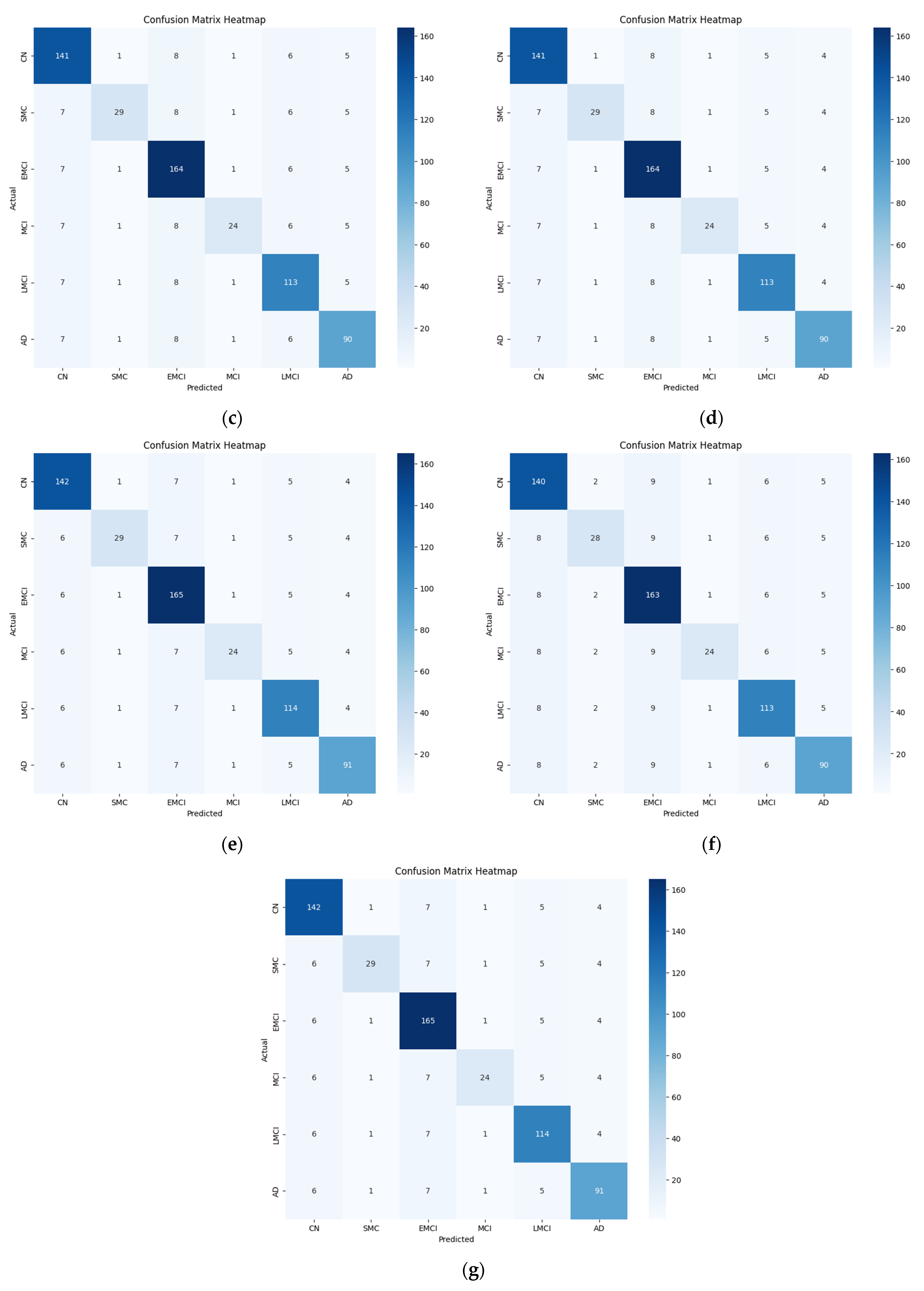
As evident in Table 4, the proposed hybrid model performed well in the multi-stage classification of AD. However, variations in accuracy were observed across different stages in the binary classification. Notably, the classification accuracy was somewhat low for the intermediate disease stages, such as EMCI and SMC. Certain stages, such as EMCI and LMCI, are closely related, and their subtle differences in brain connectivity patterns make classification challenging as discussed in Section 4.2.2. The model may misclassify samples from adjacent disease stages because of their high intra-class similarity. In addition, the validation of the generalization ability of the model will require testing on an independent dataset. While the model achieved high accuracy on the ADNI dataset, validation using datasets such as OASIS or AIBL would enhance the reliability of the results. In future work, the model will be evaluated on additional datasets to confirm its robustness and ensure its applicability for diverse populations. These results are depicted in Figure 11, and the final confusion matrix generated from the hybrid model for multiclass classification is presented in Figure 12.

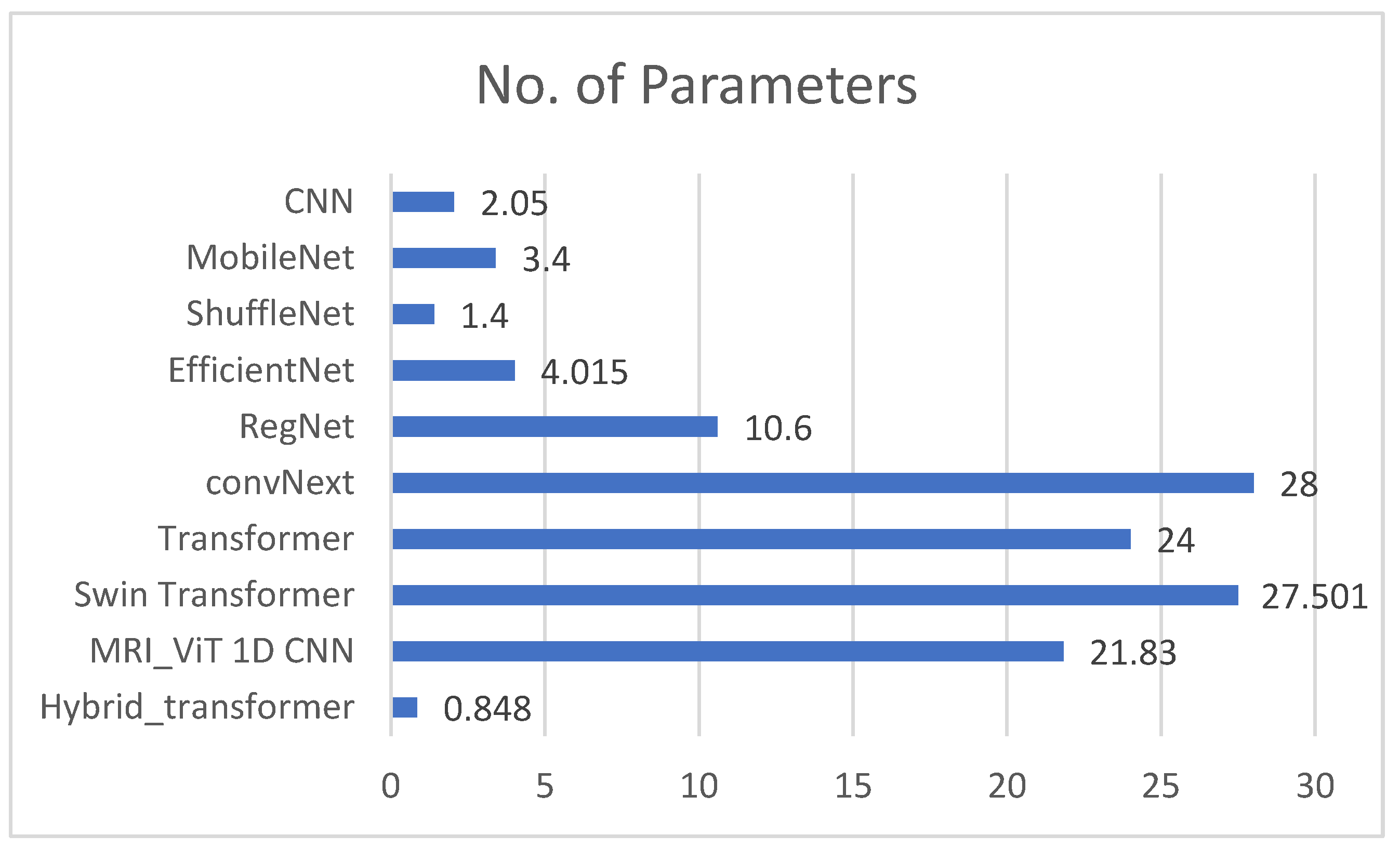
Figure 13 provides a graphical representation of the number of parameters utilized by the proposed network and the benchmark networks. The bar graph visualizes the number of parameters (in millions) used by each neural network. Each model’s complexity, in terms of learnable parameters, is compared to assess its relative size and potential capacity for capturing information from the input data. The proposed network used about 0.879 million parameters, which indicates a lightweight architecture combining CNNs and transformers. In contrast, CNN, EfficientNet-B0, MobileNet, ShuffleNet, RegNet, ConvNeXt, transformer, and Swin transformer used 2.05 million, 3.4 million, 1.4 million, 4.015 million, 10.6 million, 28 million, 24 million, and 27.501 million parameters, respectively. The point to note is that despite using fewer parameters, the proposed model achieved results that were comparable to all the benchmarks. While the number of parameters used in CNN was also small, the results were not as accurate. Similarly, although EfficientNet-B0 was optimized for efficiency, the proposed hybrid model achieved a similar or better accuracy with fewer parameters and less computational complexity. Compared to MobileNetV2 and ShuffleNetV2, the proposed model again yielded higher accuracy while remaining computationally feasible.

4.2.2. Experimental Results for Binary Classification

The results of binary classification, as presented in

Table 5. Results from benchmark networks and the proposed hybrid transformer mode model for binary classification.

Classification Task	Model	Accuracy (%)	Precision (%)	Recall (%)	F1-Score (%)	No. of Parameters
CN vs. AD	Hybrid_transformer	99.65	99.11	99.51	99.31	0.879 million
CN vs. EMCI		96.88	96.02	96.01	96.01
CN vs. MCI		98.96	98.76	98.20	98.48
CN vs. LMCI		98.44	98.45	98.53	98.49
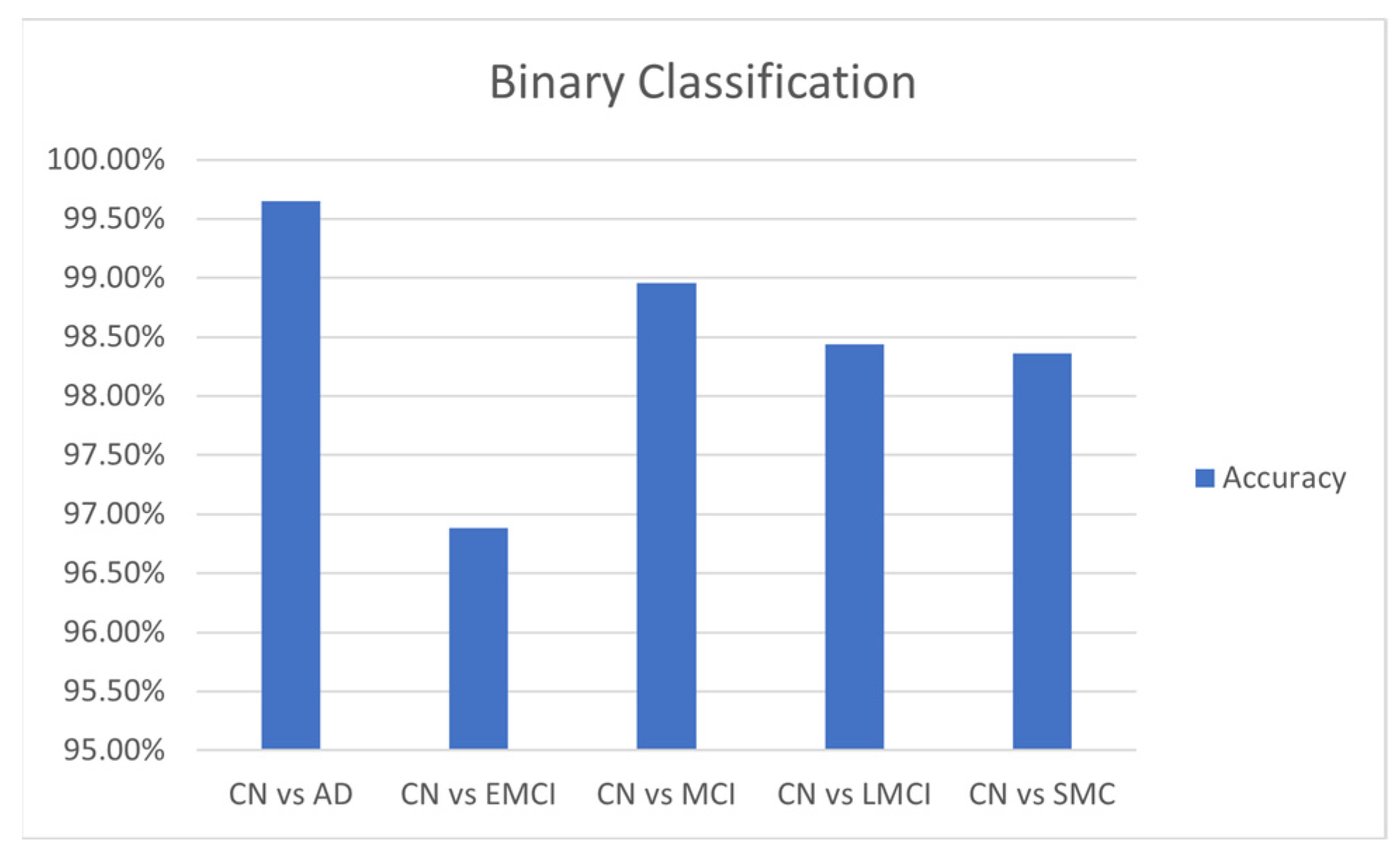
CN vs. SMC		98.36	98.20	98.41	98.30

, indicate that the hybrid transformer model adapted well to the changes across various comparison groups. In addition to its overall accuracy of 96%, the hybrid model performed well in binary classification tasks. With a batch size of 32 and a learning rate of 0.001, it achieved an average accuracy of 0.9994 and a test accuracy of 0.9965 for distinguishing between CN and AD. For differentiating CN from EMCI, the average accuracy was 0.9694, with a test accuracy of 0.9688. In the CN vs. MCI task, the model attained an average accuracy of 0.9899 and a test accuracy of 0.9896. Lastly, for CN vs. LMCI, the average accuracy was 0.9896, and the test accuracy was 0.9844. A comparison for different binary classifications is given in Figure 14.

Unlike other models, the proposed hybrid Transformer-CNN approach is specifically designed to address the unique challenges of AD classification by integrating local and global features. The CNNs extract spatial connectivity patterns from rs-fMRI data, whereas the transformers capture long-range dependencies through self-attention. This dual mechanism ensures that subtle distinctions between AD stages are recognized. As discussed in Section 3.7, the simple concatenation of features was not performed; instead, the proposed method applies interaction modeling (Equation (16)) before the final fusion (Equation (17)). This approach improves the classification accuracy by enhancing cross-modal feature learning. Moreover, hybrid models in computer vision often focus on binary classification or simpler tasks. This work specifically enhances the multi-stage classification of AD across six stages, an area that is rarely explored in depth in AD research.

The reason for selecting this variant of transformer rather than other variants, such as the Swin transformer, was its computational efficiency. Other transformer models employ hierarchical shifting windows, whereas the selected transformer variant maintains a balance between global context awareness and parameter efficiency. In addition, it is better for non-grid data. While ViTs work well for structured 2D grid-based images, rs-fMRI connectivity matrices are not strictly grid-aligned, and the selected transformer adapts better to non-grid spatial relationships in brain networks. Finally, when the proposed model was tested against ViTs and the Swin transformer, it outperformed the others in classification accuracy while keeping the computational cost lower.

4.2.3. Ablation Study Findings

As shown in

Table 6. Ablation study results.

Classification Task	Component	Accuracy (%)	Precision (%)	Recall (%)	F1-Score (%)	No. of Parameters
6-class (CN, AD, MCI, LMCI, EMCI, SMC)	CNN only	80	79	80	79	2.05 million
	Transformer	78.29	78.24	78.14	78.19	24 million
	Hybrid_transformer (concatenation only)	92	92.33	91.89	92.04	0.848 million
	Hybrid_transformer	96	96.09	96.12	96.10	0.879 million

, removing either CNNs or transformers significantly reduced the classification performance, indicating that both modules contributed meaningfully to feature extraction. The CNN-only model performs poorly for capturing long-range dependencies, whereas the transformer-only model lacks fine-grained local feature details. Similarly, combining the data in a hybrid model using multimodal fusion results in higher accuracy, demonstrating the importance of clinical data integration.

4.3. Comparison with State-of-the-Art Methods

The results of the proposed model, shown in

Table 7. Comparison of proposed methodology with state-of-the-art methods.

Study	Dataset (Modality)	Sample Size	Methods	Param (Million)	Accuracy (%)
					AD vs. MCI	AD vs. CN	AD vs. LMCI	AD vs. EMCI	AD vs. SMC	Multiclass
Q. Xiao et al. (2021) [23]	ADNI1 and ADNI-2 (MRI)	AD 93, CN 99	Multimodal representation	-	-	96.9	-	-	-	-
P. R. Buvaneswari and R. Gayathri (2021) [24]	ADNI (rs-fMRI)	AD 68 MCI 69 CN 73	Kernel-PCA for feature selection, kernel-SVR for classification	-	-	-	-	-	-	98.7% (3 stages)
H. Jia et al. (2021) [19]	ADNI (MRI)	MCI 100, AD 96, CN 97	3D PCANET for feature extraction, SVM for classification	-	86.36	92.0	-	-	-	-
M. Odusami et al. (2021) [21]	ADNI (MRI)	70k+ images of 138 subjects	ResNet 18	11	-	80.8	99.9	99.9	-	-
R. R. Janghe and Y.K Rathore (2021) [20]	ADNI (fMRI)	413 subjects	VGG16 for feature extraction, SVM for classification	138	-	99.9	-	-	-	-
R. Mohtasib et al. (2022) [18]	ADNI (MRI)	AD: 20 CN: 20	Logistic Regression and Random Forest	-	-	74	-	-	-	-
A. Loddo et al. (2022) [28]	Alzheimer MRI dataset	5k+ images	Ensemble classifier (AlexNet, ResNet101, InceptionResNetV2)	190.9	-	-	-	-	-	97.71(4 stages)
A. Alorf and M. U. G Khan (2022) [32]	ADNI (rs-fMRI)	706 fMRI scans	Stack Sparse Autoencoder and Graph convolutional network	5.846	97.03	94.17	91.73	91.45	94.43	84.03(6 stages)
El-Latif et al. (2023) [29]	Kaggle (MRI)	5k+ images	Lightweight CNN model	7.87	-	99.22	-	-	-	95.93(4 stages)
R. A. Hazarika et al. (2023) [25]	ADNI (MRI)	CN: 50, MCI: 50, AD: 50; Total images: 11,000+	Hybrid LeNet + AlexNet	12.14	-	93.58	-	-	-	83(3 stages)
M. EL-Geneedy et al. (2023) [30]	OASIS (MRI)	ND: 3200, VMD: 2240, MD: 896, MoD: 64	Shallow CNN (5 convolutional layers)	2.05	-	-	-	-	-	99.687(4 stages)
M. Odusami et al. (2023) [14]	ADNI (MRI)	AD: 50, EMCI:50, LMCI:50	Vision Transformer (ViT), DWT, VGG16	31.21	-	-	81.25	81.25	-	-
Z. Zhou et al. (2024) [26]	ADNI (fMRI)	CN: 170; AD: 170; MCI: 170	Graph Attention Network	18.24	91.16	82.26	-	-	-	69.22 (3 stages)
P. He et al. (2024) [15]	ADNI (rs-fMRI)	AD: 120; eMCI: 216; IMCI: 154 CN: 116	spatiotemporal graph transformer network (STGTN).	24.02	-	92.31	-	-	-	84.01 (eMCI vs. IMCI)
Y. Li et al. (2024) [31]	Manually collected (MRI)	6400 images (4 classes)	Transformer, Stacking Ensemble Method	25.1	-	98.51	-	-	-	97.8(4-class)
J. Chen et al. [7]	ADNI (MRI)	AD: 278, MCI: 654, CN: 518	MRI_ViT with attention-embedded 1D CNN	21.38	-	-	-	-	-	97.65(3-class)
PROPOSED	ADNI (rs-fMRI)	CN: 182 SMC: 36 EMCI: 213 LMCI: 145 MCI: 14 AD: 116	Hybrid Transformer model	0.848	98.96	99.65	98.44	96.88	98.36	96

, indicate that it outperformed state-of-the-art models such as ResNet18, the Ensemble classifier method, and the vision transformer. This was primarily due to two key factors, namely, the number of classes that could be classified and the computational resources required to accomplish the task. The ResNet18 and Ensemble methods were trained on data with fewer classes, at two and four classes, respectively, whereas the proposed Transformer-CNN was trained on a six-class problem. Even so, it achieved a high accuracy of 96.34%. This result indicates the model’s efficiency and flexibility in the multiclass case. By comparison, ResNet18 had an accuracy of 99.99%, and the Ensemble method achieved 97.71% accuracy in simple working tasks and much higher computational costs. Furthermore, concerning computational complexity, the proposed model is less costly than typical transformers, which are computationally intensive and efficient CNNs. Overall, the Transformer-CNN is guaranteed to be less complex than the vision transformer. Although other state-of-the-art methods perform well in some respects, they often require vast computational power. This point renders them unsuitable for deployment in environments with limited computational resources; for example, the model introduced by J. Chen et al. [7] used almost 21.38 million parameters, which is far more than the proposed model.

Traditional transformer models process high-dimensional input sequences, which can be computationally expensive. However, by integrating a CNN for feature extraction before applying self-attention, the sequence length was effectively reduced, which led to lower computational complexity for the transformer module. The parameters are reduced due to the hybrid design. By contrast, a standalone transformer for feature extraction would require a deeper network to capture the local and global dependencies, with higher demands regarding memory and computation. The CNN extracts local features efficiently with fewer parameters, which reduces the overall parameter count compared to a solely transformer-based approach.

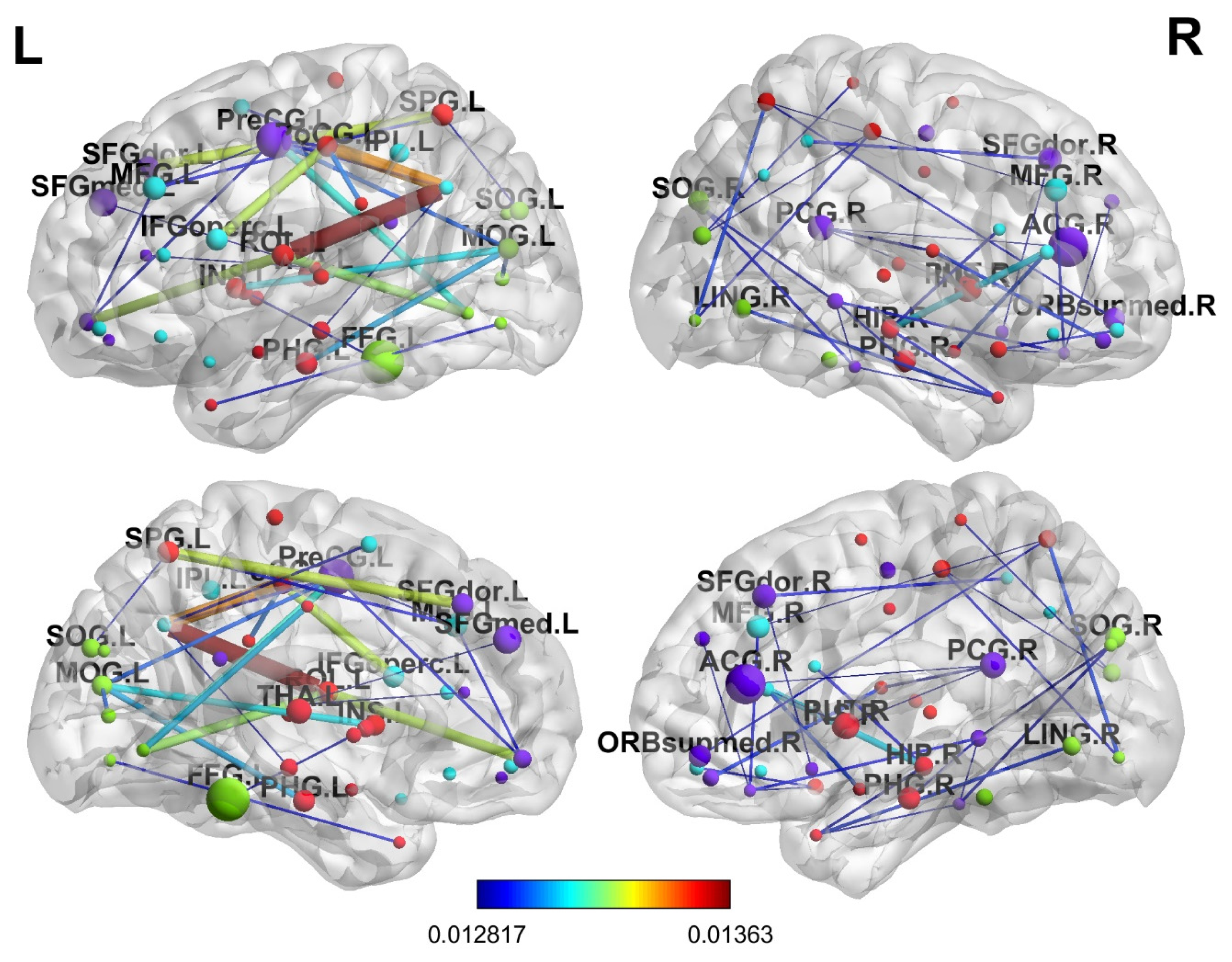
4.4. Interpretability Analysis

For in-depth interpretability analysis, the brain regions were determined in terms of the progression of AD. The final attention weight matrix of the proposed model was extracted for visualization; after the attention matrix was extracted, it was visualized using the BrainNetviewer [44]. As mentioned before, an atlas of 90 brain regions was used, which depicts various brain regions. Brain regions that received the most attention from the model included ParaHippocampal_R, which relates to memory processing; Hippocampus_R, which is critical for early AD; Amygdala_R, which affects emotional regulation; Cingulum_Ant_L, Cingulum_Mid_L, and Cingulum_Post_L, which are primarily affected in AD; and Parietal_Inf_L, which is involved in spatial cognition and is affected in the later disease stages. The same findings were reported in various other studies [45,46,47] A lateral and medial view of the brain is shown in Figure 15 and illustrates which brain regions are prioritized using the proposed model.

5. Conclusions

This study offers techniques for the multi-stage classification of AD across the six disease phases. rs-fMRI data were utilized from a renowned repository, ADNI, for this purpose. First, the rs-fMRI scans were preprocessed using various techniques, and the final output from the scans was used to generate functional connectivity matrices by applying Pearson’s correlation technique. A hybrid transformer model was adopted for binary and multiclass classification. For multiclass classification, the proposed model achieved an accuracy of 96%, surpassing several strong baselines, including ConvNext (95.82%) and Swin Transformer (95.35%) while using 30× fewer parameters than the heaviest models. For binary classification, the results were as follows: 96.88% for CN vs. EMCI, 98.36% for CN vs. SMC, 99.65% for CN vs. AD, 98.44% for CN vs. LMCI, and 98.96% for CN vs. MCI. Compared to previous studies, the proposed method performed well on the dataset. The performance is attributed to the self-attention mechanism of the transformer model, which was combined with the feature extraction power of CNN. These results validate the efficacy of the proposed hybrid architecture, which combines CNNs for local feature extraction with self-attention layers for global context modeling. In terms of other evaluation metrics, such as precision, recall, and F1-score, the proposed method achieved comparable results. Specifically, the hybrid transformer model obtained 96.09%, 96.12%, and 96.10% for precision, recall, and F1-score. These metrics were also recorded for the binary classification tasks. Overall, the results show that the proposed model is accurate. Moreover, it is lightweight and uses fewer parameters than state-of-the-art methods. The performance gains in terms of accuracy and model efficiency suggest that the proposed model is well suited for clinical applications, especially in resource-constrained environments. The lightweight nature of the model makes it suitable for real-world deployment in resource-constrained settings. In addition, the proposed methodology can potentially be adapted for the classification of other disorders involving functional brain connectivity. In the future, more robust and advanced methods can be applied for better generalization of results, and different datasets on various neurodegenerative diseases could be explored. Finally, combining rs-fMRI with other imaging modalities (e.g., structural MRI or PET scans) could provide additional insights into AD progression.