An Inertial Subgradient Extragradient Method for Efficiently Solving Fixed-Point and Equilibrium Problems in Infinite Families of Demimetric Mappings

Abstract

The primary objective of this article is to enhance the convergence rate of the extragradient method through the careful selection of inertial parameters and the design of a self-adaptive stepsize scheme. We propose an improved version of the extragradient method for approximating a common solution to pseudomonotone equilibrium and fixed-point problems that involve an infinite family of demimetric mappings in real Hilbert spaces. We establish that the iterative sequences generated by our proposed algorithms converge strongly under suitable conditions. These results substantiate the effectiveness of our approach in achieving convergence, marking a significant advancement in the extragradient method. Furthermore, we present several numerical tests to illustrate the practical efficiency of the proposed method, comparing these results with those from established methods to demonstrate the improved convergence rates and solution accuracy achieved through our approach.

1. Introduction

Let $\mathcal{Z}$ be a real Hilbert space equipped with the inner product $⟨·,·⟩$ and the corresponding norm $\parallel ·\parallel$. Denote by $\mathcal{X}$ a nonempty, closed, and convex subset of $\mathcal{Z}$. This paper focuses on identifying a common solution to both equilibrium and fixed-point problems within the framework of real Hilbert spaces. These problems have broad applications in diverse mathematical models, where equilibrium or fixed-point conditions frequently arise. As highlighted in numerous research works [1,2,3,4,5,6], these concepts are particularly relevant in practical fields such as signal processing, composite minimization, optimal control, and image restoration. Consider a bifunction $\mathcal{L}:\mathcal{Z}\times \mathcal{Z}\to \mathbb{R}$, satisfying $\mathcal{L}(x,x)=0$ for all $x\in \mathcal{Z}$. The objective of the equilibrium problem (EP) is to find a point ${\tau }^{*}\in \mathcal{X}$ such that

$$\mathcal{L}({\tau }^{*},x)\ge 0\mathrm{for}\mathrm{all}x\in \mathcal{X}.$$

(1)

Equilibrium problems (EPs) provide a comprehensive mathematical framework encompassing a range of problems, such as fixed-point problems, variational inequalities, optimization problems, saddle-point problems, complementarity problems, and Nash equilibria in non-cooperative games. The main goal of EPs is to determine equilibrium conditions that ensure the stability of a system. Solutions to EPs are particularly important in fields like economics and game theory, as demonstrated in Nash’s seminal work [7], where equilibrium is a central concept. Formally represented by (1), the equilibrium problem has garnered considerable attention and has diverse applications, including poroelasticity in petroleum engineering [8], economics [9], image reconstruction [10], telecommunications networks, public infrastructure [11], and Nash equilibria in game theory [12]. Despite their broad applicability, the formal study of EPs only began after the establishment of Ky Fan’s inequality [13]. Following this, Nikaido recognized Nash equilibria as solutions to EPs [14], while Gwinner clarified the relationships among EPs, optimization, and variational inequalities [15]. However, these early studies did not initially identify EPs as a distinct class of mathematical problems.

The primary method for addressing the problem outlined in (1), based on the auxiliary problem principle, was first introduced in [16]. This approach, commonly known as the proximal-like method, established a foundation for subsequent research into its convergence properties, as investigated in [17]. The analysis in [17] extends to cases where the equilibrium bifunction exhibits pseudo-monotonicity and satisfies Lipschitz-type conditions. The extragradient method, an iterative optimization approach for variational inequality and equilibrium problems, extends the classical gradient method by adding an extra step to improve convergence. As presented in [17], this method generates sequences $\left\{q_n\right\}$ and $\left\{p_n\right\}$ as follows:

1.

Initialization: Start from any $q_0$ in the feasible set $\mathcal{X}$.

2.

Iterative steps: Compute $p_n$ and $q_{n+1}$ using

$$\left\{\begin{array}{c}{p}_n=\underset{p\in \mathcal{X}}{argmin}\left\{\zeta \mathcal{L}(q_n,p)+{\displaystyle \frac{1}{2}}{\parallel q_n-p\parallel }^2\right\},\hfill \\ q_{n+1}=\underset{p\in \mathcal{X}}{argmin}\left\{\zeta \mathcal{L}(p_n,p)+{\displaystyle \frac{1}{2}}{\parallel q_n-p\parallel }^2\right\},\hfill \end{array}\right.$$

(2)

where $\zeta$ is a positive parameter, and $\parallel ·\parallel$ is the norm in $\mathcal{Z}$.

3.

Stopping criterion: The process stops when $p_n=q_n$, with $q_n$ as the solution to (1).

The method in (2) requires careful selection of the parameter $\zeta$, which must satisfy $0<\zeta <min\left\{{\displaystyle \frac{1}{2c^1}},{\displaystyle \frac{1}{2c^2}}\right\}$, where $c^1$ and $c^2$ are constants with Lipschitz-type conditions. The extragradient methods, as introduced by Korpelevich in [18] and further developed in [16,17], are effective in solving equilibrium problems and are widely used in optimization and variational analysis.

This paper focuses on the fixed-point problem (FPP) associated with a mapping $\mathcal{P}:\mathcal{Z}\to \mathcal{Z}$, defined as finding ${\tau }^{*}\in \mathcal{Z}$ such that $\mathcal{P}\left({\tau }^{*}\right)={\tau }^{*}$. The set of fixed points, $Fix\left(\mathcal{P}\right)$, consists of solutions to the FPP. The goal is to provide a unified solution for both the EPs and FPPs in real Hilbert spaces, with applications in areas like signal processing, network resource management, and image restoration, where constraints are often modeled as fixed-point problems. The equilibrium problem with a fixed point constraint (EPFPP) has gained significant attention, leading to various proposed solution methods, as shown in studies such as [19,20,21,22,23,24,25,26,27,28,29]. This paper addresses the following problem:

$${\tau }^{*}\in \mathcal{X}\mathrm{such}\mathrm{that}\mathcal{L}({\tau }^{*},x)\ge 0\mathrm{for}\mathrm{all}x\in \mathcal{X},\mathrm{and}{\tau }^{*}\in \bigcap _{i=1}^{+\infty }\mathrm{Fix}\left({\mathcal{P}}_i\right).$$

(3)

The method presented in (2) serves as a foundational reference in the field. Building on the work of Tran et al. [17], recent advancements in extragradient-type methods have been developed to address equilibrium problems in infinite-dimensional Hilbert spaces, with significant contributions documented in studies such as [30,31,32,33]. The approach outlined in (2) requires solving a strongly convex programming problem on the set $\mathcal{X}$ twice per iteration, which can substantially increase computational costs, particularly when dealing with complex sets $\mathcal{X}$. To overcome this challenge, adaptations of the subgradient extragradient method, as proposed by Censor, Gibali, and Reich [34,35], have been introduced for equilibrium problems in infinite-dimensional Hilbert spaces. Notable improvements in [30,33,36] reformulate the problem on $\mathcal{X}$ as a half-space optimization at each iteration, thereby improving computational efficiency compared to traditional methods. It is important to note that the implementation of the method in (2) requires prior knowledge of the Lipschitz constants associated with the bifunction $\mathcal{L}$. However, obtaining such information can be challenging in practical applications. Self-adaptive methods are particularly advantageous in situations where the Lipschitz constants are unknown, as they are specifically designed to operate effectively without relying on this information.

Motivated by the methods presented in [37,38], we propose a novel inertial algorithm that is both simple and efficient for approximating solutions to equilibrium and fixed-point problems, utilizing a subgradient extragradient approach. The main contributions of this study are summarized as follows:

(a)

The proposed algorithm enhances the iterative process by incorporating inertial terms, which introduce momentum-like effects. The inclusion of these inertial components significantly accelerates the convergence rate of the iterative sequence.

(b)

The method employs a monotonic stepsize scheme, enabling dynamic adjustment of the stepsize throughout the iterative process. This adaptive stepsize strategy eliminates the need for prior knowledge of the Lipschitz constants of the bifunction, which are often difficult to determine in practical applications.

(c)

Our study demonstrates that the sequence generated by the method we propose exhibits strong convergence to the unified fixed points within the framework of demimetric mappings. These fixed points correspond to solutions of equilibrium problems associated with pseudomonotone operators, which play a crucial role in various mathematical models. The observed convergence to these common fixed points highlights the versatility and effectiveness of the algorithm in solving a broad class of equilibrium problems.

(d)

To evaluate the effectiveness of the proposed approach, we conduct a series of extensive numerical experiments. These experiments involve solving several instances of equilibrium and fixed-point problems using our algorithm and comparing its performance with other methods available in the literature. Through detailed numerical examples and a comparative analysis, we illustrate the superior performance and efficiency of our method in terms of convergence speed, accuracy, and robustness.

This paper is organized as follows: Section 2 reviews preliminary results, Section 3 discusses the convergence properties of the proposed algorithms, Section 4 presents computational experiments comparing their performance with existing methods, and Section 5 concludes the paper.

2. Preliminaries

Let $\mathcal{X}$ be a nonempty, closed, and convex subset of the real Hilbert space $\mathcal{Z}$. We denote weak convergence by $u_n\rightharpoonup u$ and strong convergence by $u_n\to u$. For any $h_1,h_2\in \mathcal{Z}$ and scalar $e\in \mathbb{R}$, the following properties hold [39]:

(i)

${\parallel h_1+h_2\parallel }^2={\parallel h_1\parallel }^2+2⟨h_1,h_2⟩+{\parallel h_2\parallel }^2.$

(ii)

${\parallel h_1+h_2\parallel }^2\le {\parallel h_1\parallel }^2+2⟨h_2,h_1+h_2⟩.$

(iii)

${\parallel e{h}_1+(1-e)h_2\parallel }^2=e{\parallel h_1\parallel }^2+(1-e){\parallel h_2\parallel }^2-e(1-e){\parallel h_1-h_2\parallel }^2.$

Definition 1 

([39]). Let $\mathcal{X}$ be a subset of a real Hilbert space $\mathcal{Z}$, and let $\varkappa :\mathcal{X}\to \mathbb{R}$ be a convex function.

(i)

The normal cone at $h_1\in \mathcal{X}$ is 

$$N_{\mathcal{X}}\left(h_1\right)=\{h_3\in \mathcal{Z}\mid ⟨h_3,h_2-h_1⟩\le 0,\forall h_2\in \mathcal{X}\}.$$

(ii)

The subdifferential of ϰ at $h_1\in \mathcal{X}$ is

$$\partial \varkappa \left(h_1\right)=\{h_3\in \mathcal{Z}\mid \varkappa \left(h_2\right)-\varkappa \left(h_1\right)\ge ⟨h_3,h_2-h_1⟩,\forall h_2\in \mathcal{X}\}.$$

Definition 2 

([40]). Let $\mathcal{L}:\mathcal{X}\times \mathcal{X}\to \mathbb{R}$ be a bifunction on $\mathcal{X}$ with a positive constant $\gamma >0$. We say that $\mathcal{L}$ is

(i)

Strongly monotone if

$$\mathcal{L}(h_1,h_2)+\mathcal{L}(h_2,h_1)\le -\gamma {\parallel h_1-h_2\parallel }^2,\forall h_1,h_2\in \mathcal{X},$$

(ii)

Monotone if

$$\mathcal{L}(h_1,h_2)+\mathcal{L}(h_2,h_1)\le 0,\forall h_1,h_2\in \mathcal{X},$$

(iii)

Strongly pseudomonotone if

$$\mathcal{L}(h_1,h_2)\ge 0\Rightarrow \mathcal{L}(h_2,h_1)\le -\gamma {\parallel h_1-h_2\parallel }^2,\forall h_1,h_2\in \mathcal{X},$$

(iv)

Pseudomonotone if

$$\mathcal{L}(h_1,h_2)\ge 0\Rightarrow \mathcal{L}(h_2,h_1)\le 0,\forall h_1,h_2\in \mathcal{X},$$

(v)

Lipschitz-type continuous if there exist constants $c^1,c^2>0$ such that

$$\mathcal{L}(h_1,h_3)\le \mathcal{L}(h_1,h_2)+\mathcal{L}(h_2,h_3)+c^1{\parallel h_1-h_2\parallel }^2+c^2{\parallel h_2-h_3\parallel }^2,\forall h_1,h_2,h_3\in \mathcal{X}.$$

Definition 3 

([41]). Let $\mathcal{P}:\mathcal{X}\to \mathcal{X}$ with $Fix\left(\mathcal{P}\right)\ne \varnothing$. The mapping $\mathcal{P}$ is classified as follows:

(i)

Nonexpansive if

$$\parallel \mathcal{P}\left(h_1\right)-\mathcal{P}\left(h_2\right)\parallel \le \parallel h_1-h_2\parallel ,\forall h_1,h_2\in \mathcal{X}.$$

(ii)

Quasi-nonexpansive if

$$\parallel \mathcal{P}\left(h_1\right)-h_3\parallel \le \parallel h_1-h_3\parallel ,\forall h_3\in Fix\left(\mathcal{P}\right)and{h}_1\in \mathcal{X}.$$

(iii)

$\mathit{k}$-Demicontractive if for $0\le k<1$,

$$\parallel \mathcal{P}\left(h_1\right)-h_3{\parallel }^2\le \parallel h_1-h_3{\parallel }^2+k{\parallel (I-\mathcal{P})\left(h_1\right)\parallel }^2,\forall h_3\in Fix\left(\mathcal{P}\right),h_1\in \mathcal{X}.$$

(iv)

$\mathit{k}$-Demimetric if $Fix\left(\mathcal{P}\right)\ne \varnothing$ and for $-\infty \le k<1$

$$⟨h_1-h_2,h_1-\mathcal{P}\left(h_1\right)⟩\ge {\displaystyle \frac{1-k}{2}}{\parallel h_1-\mathcal{P}\left(h_1\right)\parallel }^2,\forall h_1\in \mathcal{X},h_2\in Fix\left(\mathcal{P}\right).$$

Lemma 1 

([37]). Let $\varkappa :\mathcal{X}\to \mathbb{R}$ be a subdifferentiable, convex, and lower semi-continuous function on $\mathcal{X}$. An element $h_1\in \mathcal{X}$ is a minimizer of ϰ if and only if

$$0\in \partial \varkappa \left(h_1\right)+N_{\mathcal{X}}\left(h_1\right),$$

where $\partial \varkappa \left(h_1\right)$ is the subdifferential of ϰ at $h_1$, and $N_{\mathcal{X}}\left(h_1\right)$ is the normal cone to $\mathcal{X}$ at $h_1$.

Lemma 2 

([29]). Let $\mathcal{Z}$ be a Hilbert space and $\mathcal{X}\subseteq \mathcal{Z}$ a nonempty, closed, and convex subset. Let $k\in (-\infty ,0)$, and define the mapping $\mathcal{P}:\mathcal{X}\to \mathcal{Z}$ satisfying the k-demimetric condition, ensuring that $Fix\left(\mathcal{P}\right)$ is non-empty. Let $\zeta \in (0,1-k]$, and define $\mathcal{S}=(1-\zeta )I+\zeta \mathcal{P}$. Then,

(i)

$Fix\left(\mathcal{P}\right)=Fix\left(\mathcal{S}\right)$;

(ii)

$Fix\left(\mathcal{P}\right)$ is closed and convex;

(iii)

$\mathcal{S}$ is quasi-nonexpansive from $\mathcal{X}$ to $\mathcal{Z}$.

Lemma 3 

([42]). Let $\mathcal{Z}$ be a Hilbert space and $\mathcal{X}$ a nonempty closed convex subset of $\mathcal{Z}$. Consider a sequence of mappings ${\left\{{\mathcal{P}}_i\right\}}_{i=1}^{\infty }:\mathcal{X}\to \mathcal{Z}$, where each ${\mathcal{P}}_i$ is a ${\sigma }_i$-demimetric mapping with $sup\{{\sigma }_i:i\in \mathbb{N}\}<1$ and ${\bigcap }_{i=1}^{\infty }\mathrm{Fix}\left({\mathcal{P}}_i\right)\ne \varnothing$. Let ${\left\{{\varphi }_i\right\}}_{i=1}^{\infty }$ be a positive sequence with ${\sum }_{i=1}^{\infty }{\varphi }_i=1$. Then, the mapping   

$$\sum _{i=1}^{\infty }{\varphi }_i{\mathcal{P}}_i:\mathcal{X}\to \mathcal{Z}$$

is a σ-demimetric mapping with $\sigma =sup\{{\sigma }_i:i\in \mathbb{N}\}$, and $\mathrm{Fix}\left({\sum }_{i=1}^{\infty }{\varphi }_i{\mathcal{P}}_i\right)={\bigcap }_{i=1}^{\infty }\mathrm{Fix}\left({\mathcal{P}}_i\right).$

Lemma 4 

([43]). Let $\mathcal{P}:\mathcal{X}\to \mathcal{Z}$ be a nonexpansive mapping. Then, $\mathcal{P}$ is demiclosed on $\mathcal{X}$ if, for any sequence $\left\{u_n\right\}$ weakly converging to $u\in \mathcal{X}$, with $\{u_n-\mathcal{P}{u}_n\}$ strongly converging to 0, we have $u\in Fix\left(\mathcal{P}\right)$.

Lemma 5 

([44]). Let $\left\{a_n\right\}$ be a sequence of non-negative real numbers, and $\left\{{\beta }_n\right\}$ a sequence in $(0,1)$ with ${\sum }_{n=1}^{\infty }{\beta }_n=\infty$. Suppose $\left\{{\mathfrak{b}}_n\right\}$ is a sequence such that for all $n\ge 1$,

$$a_{n+1}\le (1-{\beta }_n)a_n+{\beta }_n{\mathfrak{b}}_n.$$

If for any subsequence $\left\{a_{n_k}\right\}$,

$$\underset{k\to \infty }{lim\; inf}(a_{n_k+1}-a_{n_k})\ge 0\mathit{and}\underset{k\to \infty }{lim\; sup}{\mathfrak{b}}_{n_k}\le 0,$$

then ${lim}_{n\to \infty }{a}_n=0.$

3. Main Results

This section presents a novel algorithm for solving the problem in (3). The proposed method combines a monotonic adaptive step-size rule with an inertial subgradient extragradient framework. By incorporating inertial techniques into a hybrid approach, the algorithm effectively addresses both EPs and FPPs, which play a fundamental role in optimization, game theory, and variational analysis. The algorithm updates the solution iteratively through a sequence of projection and minimization steps, guaranteeing convergence.

The algorithm begins with initial points $u_0,u_1\in \mathcal{X}$ and generates a sequence $\left\{u_n\right\}$ as follows. Step 1 dynamically determines the inertial term ${\wp }_n$ to balance speed and stability. Step 2 computes an intermediate point ${\nu }_n$ and minimizes a function, adjusted by regularization, to obtain $y_n$. In Step 3, a minimization over the constrained set ${\mathcal{Z}}_n$ is performed, followed by a weighted update for $u_n$. Step 4 adapts the step size ${\lambda }_{n+1}$ based on progress, enhancing efficiency and ensuring convergence.

This method integrates inertial terms with self-adaptive stepsizes, improving convergence rates for complex fixed-point and equilibrium problems. The inclusion of regularization and adaptive parameters ensures robustness and flexibility, making it suitable for diverse optimization applications. To prove convergence analysis and initialize the main method, we assume the following conditions hold.

Assumption 1. 

Let $\mathcal{Z}$ be a real Hilbert space, and $\mathcal{X}\subset \mathcal{Z}$ a non-empty, closed, convex set. The following conditions hold:

(c1)

The bifunction $\mathcal{L}$ is pseudomonotone and Lipschitz continuous on $\mathcal{X}$.

(c2)

${\left\{{\mathcal{P}}_i\right\}}_{i=1}^{+\infty }$ is an infinite family of ${\sigma }_i$-demimetric mappings, each demiclosed at zero, with ${\sigma }_i\in (-\infty ,1)$. Let $\sigma =sup\{{\sigma }_i:i\ge 1\}\le 1$. Define $\Psi ={\sum }_{i=1}^{+\infty }{\gamma }_i{\mathcal{P}}_i$, where ${\sum }_{i=1}^{+\infty }{\gamma }_i=1$, and conclude from Lemma 3 that Ψ is a σ-demimetric mapping. Define $\mathcal{G}=(1-\kappa )I+\kappa \Psi$ with $\kappa \in (0,1-\sigma ]$.

(c3)

The sequence $\left\{{\mu }_n\right\}$ is positive and satisfies ${\mu }_n=o\left({\beta }_n\right)$, with ${lim}_{n\to +\infty }{\displaystyle \frac{{\mu }_n}{{\beta }_n}}=0$. Additionally, there exists $a>0$ such that ${\alpha }_n\subset (a,1-{\beta }_n)$, where $\left\{{\beta }_n\right\}\subset (0,1)$, ${lim}_{n\to +\infty }{\beta }_n=0$, and ${\sum }_{n=1}^{+\infty }{\beta }_n=+\infty$.

(c4)

The set $\Gamma =EP(\mathcal{L},\mathcal{X})\cap \mathrm{Fix}(\Psi )$ is non-empty, i.e., $\Gamma \ne \varnothing$.

The following lemma establishes that the sequence $\left\{{\lambda }_n\right\}$ defined in (6), which represents the stepsize in the algorithm, is well-defined and bounded. This property is essential for the performance of the algorithm, as the boundedness of $\left\{{\lambda }_n\right\}$ ensures the stability of the iterative process and is critical for demonstrating the convergence of the method.

Lemma 6. 

The sequence $\left\{{\lambda }_n\right\}$ generated by the update rule in (6) from Algorithm 1 is non-increasing and satisfies the following inequality:

$${\lambda }_1\ge {\lambda }_n\ge min\left\{{\displaystyle \frac{\mu }{2max\{c^1,c^2\}}},{\lambda }_1\right\}.$$

Proof. 

From (6), it is evident that the sequence $\left\{{\lambda }_n\right\}$ is non-increasing. Additionally, by applying the Lipschitz condition to the function $\mathcal{L}$, we obtain the following inequality:

$$\begin{array}{cc}\hfill {\displaystyle \frac{\mu }{2}}{\displaystyle \frac{\parallel {\nu }_n-y_n{\parallel }^2+{\parallel y_n-q_n\parallel }^2}{\mathcal{L}({\nu }_n,q_n)-\mathcal{L}({\nu }_n,y_n)-\mathcal{L}(y_n,q_n)}}& \ge {\displaystyle \frac{\mu }{2}}{\displaystyle \frac{\parallel {\nu }_n-y_n{\parallel }^2+{\parallel y_n-q_n\parallel }^2}{c^1\parallel {\nu }_n-y_n{\parallel }^2+c^2{\parallel q_n-y_n\parallel }^2}}\hfill \\ \hfill & \ge {\displaystyle \frac{\mu }{2max\{c^1,c^2\}}}.\hfill \end{array}$$

Thus, the sequence $\left\{{\lambda }_n\right\}$ is non-increasing and bounded below. Furthermore, we have ${lim}_{n\to \infty }{\lambda }_n=\zeta$.    □

Algorithm 1 Inertial Hybrid Algorithm for Fixed-Point and Equilibrium Problems

1: Initialization: Choose ${\lambda }_1>0$, $\wp >0$, $\mu \in (0,1)$, and $\rho \in (0,1]$. Let $u_0,u_1\in \mathcal{Z}$ be arbitrary initial points. 2: while$n\ge 1$do 3:     Step 1: For the iterates $u_{n-1}$ and $u_n$, and a positive constant ℘, choose ${\wp }_n$ such that $0\le {\wp }_n\le {\widehat{\wp }}_n$, where $${\widehat{\wp }}_n=\left\{\begin{array}{ll}min\{\wp ,{\displaystyle \frac{{\mu }_n}{\parallel u_n-u_{n-1}\parallel }}\},& \mathrm{if}{u}_n\ne u_{n-1},\\ \wp ,& \mathrm{otherwise}.\end{array}\right.$$ (4) 4:     Step 2: Compute $$\left\{\begin{array}{l}{\nu }_n=u_n+{\wp }_n(u_n-u_{n-1}),\\ y_n=\underset{y\in \mathcal{X}}{argmin}\left\{{\lambda }_n\mathcal{L}({\nu }_n,y)+{\displaystyle \frac{1}{2}}{\parallel {\nu }_n-y\parallel }^2\right\}.\end{array}\right.$$ 5:     Step 3: Compute $$\left\{\begin{array}{l}{q}_n=\underset{y\in {\mathcal{Z}}_n}{argmin}\left\{\rho {\lambda }_n\mathcal{L}(y_n,y)+{\displaystyle \frac{1}{2}}{\parallel {\nu }_n-y\parallel }^2\right\},\\ z_n=(1-{\beta }_n)q_n,\\ u_{n+1}=(1-{\alpha }_n)z_n+{\alpha }_n\mathcal{G}{z}_n,n\in \mathbb{N},\end{array}\right.$$ (5) where ${\mathcal{Z}}_n=\{z\in \mathcal{Z}:⟨{\nu }_n-{\lambda }_n{\mathcal{U}}_n-y_n,z-y_n⟩\le 0\}$ and ${\mathcal{U}}_n\in {\partial }_2\mathcal{L}({\nu }_n,y_n)$. 6:     Step 4: Update ${\lambda }_{n+1}$ as follows $${\lambda }_{n+1}=\left\{\begin{array}{ll}min\left\{{\lambda }_n,{\displaystyle \frac{\mu \parallel {\nu }_n-y_n{\parallel }^2+\mu {\parallel y_n-q_n\parallel }^2}{2\left[\mathcal{L}({\nu }_n,q_n)-\mathcal{L}({\nu }_n,y_n)-\mathcal{L}(y_n,q_n)\right]}}\right\},& \mathrm{if}\mathcal{L}({\nu }_n,q_n)-\mathcal{L}({\nu }_n,y_n)-\mathcal{L}(y_n,q_n)>0,\hfill \\ {\lambda }_n,& \mathrm{otherwise}.\end{array}\right.$$ (6) 7: end while

Remark 1. 

From condition (c3) in Assumption 1, we have that ${\mu }_n=o\left({\beta }_n\right)$, which implies that ${lim}_{n\to \infty }{\displaystyle \frac{{\mu }_n}{{\beta }_n}}=0$. Furthermore, from Equation (4), it follows that ${\wp }_n\le \overline{\wp }\le {\displaystyle \frac{{\mu }_n}{\parallel u_n-u_{n-1}\parallel }}$ for all $n\ge 1$, provided that $u_n\ne u_{n-1}$. Consequently, we obtain

$${\displaystyle \frac{{\wp }_n}{{\beta }_n}}\parallel u_n-u_{n-1}\parallel \le {\displaystyle \frac{{\mu }_n}{{\beta }_n}}\to 0asn\to \infty .$$

(7)

The following lemma is crucial for establishing the boundedness of the iterative sequence, which is essential for confirming the strong convergence of the proposed sequence to a common solution.

Lemma 7. 

Consider the sequences $\left\{q_n\right\}$, $\left\{{\nu }_n\right\}$, and $\left\{y_n\right\}$ generated by Algorithm 1. For every ${\tau }^{*}\in \Gamma$, it holds that

$$\parallel q_n-{\tau }^{*}{\parallel }^2\le \parallel {\nu }_n-{\tau }^{*}{\parallel }^2-(1-\rho )\parallel {\nu }_n-q_n{\parallel }^2-\rho \left(1-{\displaystyle \frac{\mu {\lambda }_n}{{\lambda }_{n+1}}}\right)\parallel {\nu }_n-y_n{\parallel }^2-\rho \left(1-{\displaystyle \frac{\mu {\lambda }_n}{{\lambda }_{n+1}}}\right){\parallel q_n-y_n\parallel }^2.$$

Proof. 

Using Lemma 1, we establish that

$$0\in {\partial }_2\left(\rho {\lambda }_n\mathcal{L}(y_n,·)+{\displaystyle \frac{1}{2}}{\parallel {\nu }_n-·\parallel }^2\right)\left(q_n\right)+N_{{\mathcal{Z}}_n}\left(q_n\right).$$

Consequently, there exist elements $w\in \partial \mathcal{L}(y_n,q_n)$ and $\overline{w}\in N_{{\mathcal{Z}}_n}\left(q_n\right)$ such that

$$\rho {\lambda }_{n}w+q_n-{\nu }_n+\overline{w}=0.$$

This leads us to the following expression:

$$⟨{\nu }_n-q_n,y-q_n⟩=\rho {\lambda }_n⟨w,y-q_n⟩+⟨\overline{w},y-q_n⟩,\forall y\in {\mathcal{Z}}_n.$$

Since $\overline{w}\in N_{{\mathcal{Z}}_n}\left(q_n\right)$, we conclude that $⟨\overline{w},y-q_n⟩\le 0$ for all $y\in {\mathcal{Z}}_n$. This yields

$$\rho {\lambda }_n⟨w,y-q_n⟩\ge ⟨{\nu }_n-q_n,y-q_n⟩,\forall y\in {\mathcal{Z}}_n.$$

(8)

Given that $w\in \partial \mathcal{L}(y_n,q_n)$, we obtain

$$\mathcal{L}(y_n,y)-\mathcal{L}(y_n,q_n)\ge ⟨w,y-q_n⟩,\forall y\in {\mathcal{Z}}_n.$$

(9)

By combining (8) and (9), we derive

$$\rho {\lambda }_n\left(\mathcal{L}(y_n,y)-\mathcal{L}(y_n,q_n)\right)\ge ⟨{\nu }_n-q_n,y-q_n⟩,\forall y\in {\mathcal{Z}}_n.$$

(10)

Substituting $y={\tau }^{*}$ into (10), we obtain

$$\rho {\lambda }_n\left(\mathcal{L}(y_n,{\tau }^{*})-\mathcal{L}(y_n,q_n)\right)\ge ⟨{\nu }_n-q_n,{\tau }^{*}-q_n⟩.$$

(11)

Since ${\tau }^{*}\in EP(\mathcal{L},\mathcal{X})$, we know that $\mathcal{L}({\tau }^{*},y_n)\ge 0$. Given the pseudomonotonicity of the bifunction $\mathcal{L}$, it follows that $\mathcal{L}(y_n,{\tau }^{*})\le 0$. Therefore, based on (11), we can infer

$$⟨{\nu }_n-q_n,q_n-{\tau }^{*}⟩\ge \rho {\lambda }_n\mathcal{L}(y_n,q_n).$$

(12)

From the definition of the half-space ${\mathcal{Z}}_n$, we obtain

$${\lambda }_n⟨{\mathcal{U}}_n,q_n-y_n⟩\ge ⟨{\nu }_n-y_n,q_n-y_n⟩.$$

(13)

Since ${\mathcal{U}}_n\in \partial \mathcal{L}({\nu }_n,y_n)$, it follows that

$$\mathcal{L}({\nu }_n,y)-\mathcal{L}({\nu }_n,y_n)\ge ⟨{\mathcal{U}}_n,y-y_n⟩,\forall y\in \mathcal{Z}.$$

Substituting $y=q_n$ into this inequality, we obtain

$$\mathcal{L}({\nu }_n,q_n)-\mathcal{L}({\nu }_n,y_n)\ge ⟨{\mathcal{U}}_n,q_n-y_n⟩,\forall y\in \mathcal{Z}.$$

(14)

Combining (13) and (14), we obtain

$${\lambda }_n\left(\mathcal{L}({\nu }_n,q_n)-\mathcal{L}({\nu }_n,y_n)\right)\ge ⟨{\nu }_n-y_n,q_n-y_n⟩.$$

(15)

Using the definition of ${\lambda }_{n+1}$, we derive the following inequality:

$${\lambda }_{n+1}\left(\mathcal{L}({\nu }_n,q_n)-\mathcal{L}({\nu }_n,y_n)-\mathcal{L}(y_n,q_n)\right)\le {\displaystyle \frac{\mu }{2}}\left(\parallel {\nu }_n-y_n{\parallel }^2+{\parallel q_n-y_n\parallel }^2\right),$$

(16)

which can also be expressed as

$${\lambda }_n\left(\mathcal{L}({\nu }_n,q_n)-\mathcal{L}({\nu }_n,y_n)-\mathcal{L}(y_n,q_n)\right)\le {\displaystyle \frac{{\lambda }_n}{{\lambda }_{n+1}}}{\displaystyle \frac{\mu }{2}}\left(\parallel {\nu }_n-y_n{\parallel }^2+{\parallel q_n-y_n\parallel }^2\right).$$

(17)

Substituting (17) into (15), we obtain

$$⟨{\nu }_n-y_n,q_n-y_n⟩\le {\lambda }_n\mathcal{L}(y_n,q_n)+{\displaystyle \frac{{\lambda }_n}{{\lambda }_{n+1}}}{\displaystyle \frac{\mu }{2}}\left(\parallel {\nu }_n-y_n{\parallel }^2+{\parallel q_n-y_n\parallel }^2\right).$$

(18)

Combining (12) and (18), we obtain

$$⟨{\nu }_n-y_n,q_n-y_n⟩\le {\displaystyle \frac{1}{\rho }}⟨{\nu }_n-q_n,q_n-{\tau }^{*}⟩+{\displaystyle \frac{{\lambda }_n}{{\lambda }_{n+1}}}{\displaystyle \frac{\mu }{2}}\left(\parallel {\nu }_n-y_n{\parallel }^2+{\parallel q_n-y_n\parallel }^2\right).$$

(19)

Additionally, we have the following:

$$2⟨{\nu }_n-q_n,q_n-{\tau }^{*}⟩=\parallel {\nu }_n-{\tau }^{*}{\parallel }^2-\parallel q_n-{\nu }_n{\parallel }^2-{\parallel q_n-{\tau }^{*}\parallel }^2,$$

(20)

and

$$2⟨{\nu }_n-y_n,q_n-y_n⟩=\parallel {\nu }_n-y_n{\parallel }^2+\parallel q_n-y_n{\parallel }^2-{\parallel {\nu }_n-q_n\parallel }^2.$$

(21)

By substituting expressions (20) and (21) into Equation (19), we deduce

$$\begin{array}{cc}\hfill \parallel {\nu }_n-y_n{\parallel }^2+\parallel q_n-y_n{\parallel }^2-{\parallel {\nu }_n-q_n\parallel }^2& \le {\displaystyle \frac{1}{\rho }}\left(\parallel {\nu }_n-{\tau }^{*}{\parallel }^2-\parallel q_n-{\nu }_n{\parallel }^2-{\parallel q_n-{\tau }^{*}\parallel }^2\right)\hfill \\ \hfill & +{\displaystyle \frac{{\lambda }_n}{{\lambda }_{n+1}}}\mu \left(\parallel {\nu }_n-y_n{\parallel }^2+{\parallel q_n-y_n\parallel }^2\right),\hfill \end{array}$$

which is equivalent to

$$\parallel q_n-{\tau }^{*}{\parallel }^2\le \parallel {\nu }_n-{\tau }^{*}{\parallel }^2-(1-\rho )\parallel {\nu }_n-q_n{\parallel }^2-\rho \left(1-{\displaystyle \frac{\mu {\lambda }_n}{{\lambda }_{n+1}}}\right)\parallel {\nu }_n-y_n{\parallel }^2-\rho \left(1-{\displaystyle \frac{\mu {\lambda }_n}{{\lambda }_{n+1}}}\right){\parallel q_n-y_n\parallel }^2.$$

   □

The following theorem constitutes the main result of our study. It establishes that the sequence generated by the proposed method converges strongly to a unique solution of the problem (3) within the solution set $\Gamma$. To prove the strong convergence of the iterative sequence, we employ the central theorem stated below, which guarantees both the boundedness of the sequence and its strong convergence to a common solution.

Theorem 1. 

Let $\left\{u_n\right\}$ be the sequence generated by Algorithm 1 under the conditions outlined in Assumption 1. Then, the sequence $\left\{u_n\right\}$ converges strongly to an element $z\in \Gamma$.

Proof. 

Claim 1: The sequence $\left\{u_n\right\}$ is bounded.

Based on Lemma 7, for $\mu \in (0,1)$ and $\rho \in (0,1]$, we can derive the following inequality:

$$(1-\rho )\ge 0,\underset{n\to \infty }{lim}\rho \left(1-{\displaystyle \frac{\mu {\lambda }_n}{{\lambda }_{n+1}}}\right)>0.$$

(22)

By combining (22) with Lemma 7, for every ${\tau }^{*}\in \Gamma$, we obtain

$$\parallel q_n-{\tau }^{*}\parallel \le \parallel {\nu }_n-{\tau }^{*}\parallel .$$

(23)

Considering the definition of the sequence $\left\{{\nu }_n\right\}$, we find

$$\begin{array}{c}\hfill \begin{array}{cc}\hfill \parallel {\nu }_n-{\tau }^{*}\parallel & = \parallel u_n-{\tau }^{*}+{\wp }_n(u_n-u_{n+1})\parallel \hfill \\ \hfill & \le \parallel u_n-{\tau }^{*}\parallel +{\beta }_n\left({\displaystyle \frac{{\wp }_n}{{\beta }_n}}\parallel u_n-u_{n+1}\parallel \right).\hfill \end{array}\end{array}$$

(24)

Given that the sequence $\left\{{\displaystyle \frac{{\wp }_n}{{\beta }_n}}\parallel u_n-u_{n+1}\parallel \right\}$ converges to zero, as stated in Remark 1, there exists a positive constant $\mathcal{K}$ such that

$$\left\{{\displaystyle \frac{{\wp }_n}{{\beta }_n}}\parallel u_n-u_{n+1}\parallel \right\}\le \mathcal{K}$$

for all $n\ge 1$. Consequently, we have

$$\parallel {\nu }_n-{\tau }^{*}\parallel \le \parallel u_n-{\tau }^{*}\parallel +{\beta }_n\mathcal{K}.$$

(25)

Thus, by combining (23) and (25), we conclude that

$$\parallel q_n-{\tau }^{*}\parallel \le \parallel u_n-{\tau }^{*}\parallel +{\beta }_n\mathcal{K}.$$

From the definition of the sequence $\left\{z_n\right\}$ and utilizing (23), we derive the following inequalities:

$$\begin{array}{cc}\hfill \parallel z_n-{\tau }^{*}\parallel & = \parallel (1-{\beta }_n)q_n-{\tau }^{*}\parallel \hfill \\ \hfill & \le (1-{\beta }_n)\parallel q_n-{\tau }^{*}\parallel +{\beta }_n\parallel {\tau }^{*}\parallel \hfill \\ \hfill & \le (1-{\beta }_n)\parallel u_n-{\tau }^{*}\parallel +{\beta }_n[\parallel {\tau }^{*}\parallel +\mathcal{K}].\hfill \end{array}$$

Given that $\Psi :={\sum }_{i=1}^{\infty }{\gamma }_i{\mathcal{P}}_i$ satisfies the condition of being a $\sigma$-demimetric as per Assumption 1(c2), and applying Lemma 2, we assert that $\mathcal{G}:=(1-\kappa )I+\kappa \Psi$ is a quasinonexpansive mapping. Therefore, from the previous inequality and the definition of $\left\{u_{n+1}\right\}$, we have

$$\begin{array}{cc}\hfill \parallel u_{n+1}-{\tau }^{*}\parallel & = \parallel (1-{\alpha }_n)z_n+{\alpha }_n\mathcal{G}{z}_n-{\tau }^{*}\parallel \hfill \\ \hfill & \le (1-{\alpha }_n)\parallel z_n-{\tau }^{*}\parallel +{\alpha }_n\parallel \mathcal{G}{z}_n-{\tau }^{*}\parallel \hfill \\ \hfill & \le (1-{\alpha }_n)\parallel z_n-{\tau }^{*}\parallel +{\alpha }_n\parallel z_n-{\tau }^{*}\parallel \hfill \\ \hfill & = \parallel z_n-{\tau }^{*}\parallel \hfill \\ \hfill & \le (1-{\beta }_n)\parallel u_n-{\tau }^{*}\parallel +{\beta }_n[\parallel {\tau }^{*}\parallel +\mathcal{K}]\hfill \\ \hfill & \le max\{\parallel u_n-{\tau }^{*}\parallel ,\parallel {\tau }^{*}\parallel +\mathcal{K}\}\hfill \\ \hfill & ⋮\hfill \\ \hfill & \le max\{\parallel u_1-{\tau }^{*}\parallel ,\parallel {\tau }^{*}\parallel +\mathcal{K}\}.\hfill \end{array}$$

Thus, this sequence of inequalities demonstrates that $\left\{u_n\right\}$ is bounded.

Claim 2.

$$\begin{array}{cc}\hfill \parallel u_{n+1}-{\tau }^{*}{\parallel }^2& \le (1-{\beta }_n){\parallel u_n-{\tau }^{*}\parallel }^2\hfill \\ \hfill & +{\beta }_n\left((1-{\beta }_n)⟨q_n-{\tau }^{*},-{\tau }^{*}⟩+{\displaystyle \frac{{\wp }_n}{{\beta }_n}}\parallel u_n-u_{n-1}\parallel +{\beta }_n{\parallel {\tau }^{*}\parallel }^2\right).\hfill \end{array}$$

From (5) and (24), we obtain

$$\begin{array}{cc}\hfill \parallel u_{n+1}-{\tau }^{*}{\parallel }^2& = \parallel (1-{\alpha }_n)z_n+{\alpha }_n\mathcal{G}{z}_n-{\tau }^{*}{\parallel }^2\hfill \\ \hfill & \le (1-{\alpha }_n)\parallel z_n-{\tau }^{*}{\parallel }^2+{\alpha }_n\parallel \mathcal{G}{z}_n-{\tau }^{*}{\parallel }^2-{\alpha }_n(1-{\alpha }_n){\parallel \mathcal{G}{z}_n-z_n\parallel }^2\hfill \\ \hfill & \le (1-{\alpha }_n)\parallel z_n-{\tau }^{*}{\parallel }^2+{\alpha }_n\parallel z_n-{\tau }^{*}{\parallel }^2-{\alpha }_n(1-{\alpha }_n){\parallel \mathcal{G}{z}_n-z_n\parallel }^2\hfill \\ \hfill & \le \parallel (1-{\beta }_n)q_n-{\tau }^{*}{\parallel }^2-{\alpha }_n(1-{\alpha }_n){\parallel \mathcal{G}{z}_n-z_n\parallel }^2\hfill \\ \hfill & \le \parallel (1-{\beta }_n)(q_n-{\tau }^{*})-{\beta }_n{\tau }^{*}{\parallel }^2-{\alpha }_n(1-{\alpha }_n){\parallel \mathcal{G}{z}_n-z_n\parallel }^2\hfill \\ \hfill & \le (1-{\beta }_n){\parallel q_n-{\tau }^{*}\parallel }^2-{\beta }_n(1-{\beta }_n)⟨q_n-{\tau }^{*},{\tau }^{*}⟩\hfill \\ \hfill & +{\beta }_n^2\parallel {\tau }^{*}{\parallel }^2-{\alpha }_n(1-{\alpha }_n){\parallel \mathcal{G}{z}_n-z_n\parallel }^2\hfill \\ \hfill & \le (1-{\beta }_n){\parallel u_n-{\tau }^{*}\parallel }^2\hfill \\ \hfill & +{\beta }_n\left((1-{\beta }_n)⟨q_n-{\tau }^{*},-{\tau }^{*}⟩+{\displaystyle \frac{{\wp }_n}{{\beta }_n}}\parallel u_n-u_{n-1}\parallel +{\beta }_n{\parallel {\tau }^{*}\parallel }^2\right).\hfill \end{array}$$

Claim 3.

$$\begin{array}{cc}\hfill \left(1-{\displaystyle \frac{\mu {\lambda }_n}{{\lambda }_{n+1}}}\right){\parallel {\nu }_n-y_n\parallel }^2& +\left(1-{\displaystyle \frac{\mu {\lambda }_n}{{\lambda }_{n+1}}}\right){\parallel q_n-y_n\parallel }^2\hfill \\ \hfill & +{\alpha }_n(1-{\alpha }_n)\parallel \mathcal{G}{z}_n-z_n{\parallel }^2+(1-\rho ){\parallel {\nu }_n-q_n\parallel }^2\hfill \\ \hfill & \le \parallel u_n-{\tau }^{*}{\parallel }^2-\parallel u_{n+1}-{\tau }^{*}{\parallel }^2+{\beta }_n^2\parallel {\tau }^{*}{\parallel }^2+{\wp }_n\parallel u_n-u_{n-1}\parallel \hfill \\ \hfill & +{\beta }_n(1-{\beta }_n)⟨q_n-{\tau }^{*},-{\tau }^{*}⟩.\hfill \end{array}$$

By employing the definition of $\left\{u_{n+1}\right\}$ and applying Lemma 7, we derive

$$\begin{array}{cc}\hfill \parallel u_{n+1}-{\tau }^{*}{\parallel }^2& = \parallel (1-{\alpha }_n)z_n+{\alpha }_n\mathcal{G}{z}_n-{\tau }^{*}{\parallel }^2\hfill \\ \hfill & \le (1-{\alpha }_n)\parallel z_n-{\tau }^{*}{\parallel }^2+{\alpha }_n\parallel \mathcal{G}{z}_n-{\tau }^{*}{\parallel }^2-{\alpha }_n(1-{\alpha }_n){\parallel \mathcal{G}{z}_n-z_n\parallel }^2\hfill \\ \hfill & \le (1-{\alpha }_n)\parallel z_n-{\tau }^{*}{\parallel }^2+{\alpha }_n\parallel z_n-{\tau }^{*}{\parallel }^2-{\alpha }_n(1-{\alpha }_n){\parallel \mathcal{G}{z}_n-z_n\parallel }^2\hfill \\ \hfill & \le \parallel (1-{\beta }_n)q_n-{\tau }^{*}{\parallel }^2-{\alpha }_n(1-{\alpha }_n){\parallel \mathcal{G}{z}_n-z_n\parallel }^2\hfill \\ \hfill & \le \parallel (1-{\beta }_n)(q_n-{\tau }^{*})-{\beta }_n{\tau }^{*}{\parallel }^2-{\alpha }_n(1-{\alpha }_n){\parallel \mathcal{G}{z}_n-z_n\parallel }^2\hfill \\ \hfill & \le (1-{\beta }_n)\parallel q_n-{\tau }^{*}{\parallel }^2-{\beta }_n(1-{\beta }_n)⟨q_n-{\tau }^{*},{\tau }^{*}⟩+{\beta }_n^2\parallel {\tau }^{*}{\parallel }^2-{\alpha }_n(1-{\alpha }_n){\parallel \mathcal{G}{z}_n-z_n\parallel }^2\hfill \\ \hfill & \le \parallel q_n-{\tau }^{*}{\parallel }^2-{\beta }_n(1-{\beta }_n)⟨q_n-{\tau }^{*},{\tau }^{*}⟩+{\beta }_n^2\parallel {\tau }^{*}{\parallel }^2-{\alpha }_n(1-{\alpha }_n){\parallel \mathcal{G}{z}_n-z_n\parallel }^2\hfill \\ \hfill & \le \parallel {\nu }_n-{\tau }^{*}{\parallel }^2-(1-\rho )\parallel {\nu }_n-q_n{\parallel }^2-\left(1-{\displaystyle \frac{\mu {\lambda }_n}{{\lambda }_{n+1}}}\right){\parallel {\nu }_n-y_n\parallel }^2\hfill \\ \hfill & -\left(1-{\displaystyle \frac{\mu {\lambda }_n}{{\lambda }_{n+1}}}\right){\parallel q_n-y_n\parallel }^2+{\beta }_n(1-{\beta }_n)⟨q_n-{\tau }^{*},-{\tau }^{*}⟩\hfill \\ \hfill & +{\beta }_n^2\parallel {\tau }^{*}{\parallel }^2-{\alpha }_n(1-{\alpha }_n){\parallel \mathcal{G}{z}_n-z_n\parallel }^2.\hfill \end{array}$$

Thus, by using (24), we establish Claim 3.

Claim 4: The sequence generated by Algorithm 1 converges strongly to an element in Γ.

Let $\{\parallel u_{n_k}-{\tau }^{*}\parallel \}$ be a subsequence of $\{\parallel u_n-{\tau }^{*}\parallel \}$ such that

$$\underset{k\to \infty }{lim\; inf}\left(\parallel u_{n_k+1}-{\tau }^{*}\parallel -\parallel u_{n_k}-{\tau }^{*}\parallel \right)\ge 0.$$

Thus, we obtain

$$\underset{k\to \infty }{lim\; inf}\left(\parallel u_{n_k+1}-{\tau }^{*}{\parallel }^2-{\parallel u_{n_k}-{\tau }^{*}\parallel }^2\right)=\underset{k\to \infty }{lim\; inf}\left[\left(\parallel u_{n_k+1}-{\tau }^{*}\parallel -\parallel u_{n_k}-{\tau }^{*}\parallel \right)·\left(\parallel u_{n_k+1}-{\tau }^{*}\parallel +\parallel u_{n_k}-{\tau }^{*}\parallel \right)\right]\ge 0.$$

We now define the sequence $\left\{{\Delta }_n\right\}$ as follows:

$${\Delta }_n:=\left(1-{\displaystyle \frac{\mu {\lambda }_n}{{\lambda }_{n+1}}}\right)\parallel {\nu }_n-y_n{\parallel }^2+\left(1-{\displaystyle \frac{\mu {\lambda }_n}{{\lambda }_{n+1}}}\right)\parallel q_n-y_n{\parallel }^2+{\alpha }_n(1-{\alpha }_n)\parallel \mathcal{G}{z}_n-z_n{\parallel }^2+(1-\rho ){\parallel {\nu }_n-q_n\parallel }^2.$$

By employing Claim 3, we obtain

$$\begin{array}{cc}\hfill \underset{k\to \infty }{lim\; sup}{\Delta }_{n_k}& \le \underset{k\to \infty }{lim\; sup}\left(\parallel u_{n_k}-{\tau }^{*}{\parallel }^2-{\parallel u_{n_k+1}-{\tau }^{*}\parallel }^2\right)\hfill \\ \hfill & +\underset{k\to \infty }{lim\; sup}{\beta }_{n_k}((1-{\beta }_{n_k})⟨q_{n_k}-{\tau }^{*},-{\tau }^{*}⟩\hfill \\ \hfill & +{\displaystyle \frac{{\wp }_{n_k}}{{\beta }_{n_k}}}\parallel u_{n_k}-u_{n_k-1}\parallel +{\beta }_{n_k}{\parallel {\tau }^{*}\parallel }^2)\hfill \\ \hfill & \le -\underset{k\to \infty }{lim\; inf}\left(\parallel u_{n_k+1}-{\tau }^{*}{\parallel }^2-{\parallel u_{n_k}-{\tau }^{*}\parallel }^2\right)\hfill \\ \hfill & \le 0.\hfill \end{array}$$

Consequently, we obtain

$$\underset{k\to \infty }{lim}{\Delta }_{n_k}=0,$$

which leads to the following result:

$$\underset{k\to \infty }{lim}\parallel {\nu }_{n_k}-y_{n_k}\parallel = \underset{k\to \infty }{lim}\parallel q_{n_k}-y_{n_k}\parallel = \underset{k\to \infty }{lim}\parallel \mathcal{G}{z}_{n_k}-z_{n_k}\parallel = \underset{k\to \infty }{lim}\parallel {\nu }_{n_k}-q_{n_k}\parallel =0.$$

(26)

Using the definition of the sequence $\left\{{\nu }_n\right\}$ adn (7), we obtain

$$\parallel {\nu }_{n_k}-u_{n_k}\parallel ={\displaystyle \frac{{\wp }_{n_k}}{{\beta }_{n_k}}}\parallel u_{n_k}-u_{n_k-1}\parallel \to 0,\mathrm{as}k\to \infty .$$

(27)

Moreover, by the definition of $\left\{z_n\right\}$ and Assumption 1 (c3), we gain

$$\parallel z_{n_k}-q_{n_k}\parallel ={\beta }_{n_k}\parallel q_{n_k}\parallel \to 0,\mathrm{as}k\to \infty .$$

(28)

By combining (26) and (27), we deduce

$$\parallel u_{n_k}-q_{n_k}\parallel \le \parallel u_{n_k}-{\nu }_{n_k}\parallel + \parallel {\nu }_{n_k}-q_{n_k}\parallel \to 0,\mathrm{as}k\to \infty .$$

(29)

Additionally, we find

$$\parallel u_{n_k}-z_{n_k}\parallel \le \parallel u_{n_k}-q_{n_k}\parallel + \parallel q_{n_k}-z_{n_k}\parallel \to 0,\mathrm{as}k\to \infty .$$

(30)

Furthermore, from Assumption 1 condition $\left(\mathrm{c}2\right)$ and (26), we conclude

$$\underset{k\to \infty }{lim}\parallel \Psi z_{n_k}-z_{n_k}\parallel = {\displaystyle \frac{1}{\psi }}\underset{k\to \infty }{lim}\parallel \mathcal{G}{z}_{n_k}-z_{n_k}\parallel =0.$$

(31)

Given that $\left\{u_{n_k}\right\}$ is bounded, there exists a subsequence $\left\{u_{n_{k_s}}\right\}$ of $\left\{u_{n_k}\right\}$ such that $\left\{u_{n_{k_s}}\right\}$ weakly converges to $u\in \mathcal{Z}$ as $s\to \infty$. From expression (30), it follows that $\left\{z_{n_{k_s}}\right\}$ also weakly converges to $u\in \mathcal{Z}$. Moreover, by Assumption 1 condition $\left(\mathrm{c}2\right)$, the demimetric and demiclosed properties of $\Psi$ at zero, and expression (31), we conclude that $u\in \mathrm{Fix}(\Psi ):=\mathrm{Fix}\left({\sum }_{i=1}^{\infty }{\gamma }_i{\mathcal{P}}_i\right)$. Furthermore, applying Lemma 3 yields $u\in {\bigcap }_{i=1}^{\infty }\mathrm{Fix}\left({\mathcal{P}}_i\right)$. Additionally, we establish that $u\in \mathrm{EP}(\mathcal{L},\mathcal{X})$. From expressions (11) and (16), we obtain

$$\begin{array}{cc}\hfill \rho {\lambda }_{n_k}\mathcal{L}(y_{n_k},y)\ge & \rho \mathcal{L}(y_{n_k},q_{n_k})+⟨{\nu }_{n_k}-q_{n_k},y-q_{n_k}⟩\hfill \\ \hfill \ge & \rho ⟨{\nu }_{n_k}-y_{n_k},q_{n_k}-y_{n_k}⟩+⟨{\nu }_{n_k}-q_{n_k},y-q_{n_k}⟩\hfill \\ \hfill & -\rho {\displaystyle \frac{{\lambda }_{n_k}}{{\lambda }_{n_k+1}}}{\displaystyle \frac{\mu }{2}}\left(\parallel {\nu }_{n_k}-y_{n_k}{\parallel }^2+{\parallel {\nu }_{n_k}-q_{n_k}\parallel }^2\right).\hfill \end{array}$$

Since $\rho >0$ and ${lim}_{k\to \infty }{\lambda }_{n_k}=\zeta >0,$ we have

$$0\le \underset{k\to \infty }{lim\; sup}\mathcal{L}(y_{n_k},y)=\mathcal{L}(u,y),\forall y\in \mathcal{X}.$$

Thus, $u\in \mathrm{EP}(\mathcal{L},\mathcal{X})$, and hence $u\in \Gamma$. We now show that the sequence $\left\{u_n\right\}$ converges strongly to $u\in \Gamma$. Next, we have

$$\parallel u_{n_k+1}{-u\parallel }^2\le (1-{\beta }_{n_k}){\parallel u_{n_k}-u\parallel }^2+{\beta }_{n_k}\left[-2(1-{\beta }_{n_k})⟨q_{n_k}-u,u⟩+{\displaystyle \frac{{\wp }_{n_k}}{{\beta }_{n_k}}}\parallel u_{n_k}-u_{n_k-1}\parallel +{\beta }_{n_k}{\parallel u\parallel }^2\right].$$

(32)

Since the sequence $\left\{u_{n_k}\right\}$ converges weakly to u as $k\to \infty$, we have ${lim}_{k\to \infty }⟨u_{n_k}-u,u⟩=0$. This implies that

$$-2(1-{\beta }_{n_k})⟨q_{n_k}-u,u⟩+{\displaystyle \frac{{\wp }_{n_k}}{{\beta }_{n_k}}}\parallel u_{n_k}-u_{n_k-1}\parallel +{\beta }_{n_k}{\parallel u\parallel }^2\to \infty \mathrm{as}k\to \infty .$$

(33)

From inequality (32), (33) and Lemma 5, it follows that ${lim}_{n\to \infty }\parallel u_n-u\parallel =0$. Consequently, $u_n\to u\in \Gamma$.    □

Application to Solve Variational Inequalities

In this section, we apply our findings to address variational inequality problems that involve a pseudomonotone and Lipschitz continuous operator, as well as an infinite family of demimetric mappings, within the context of real Hilbert spaces. The primary objective is to establish a theorem that identifies a common solution for both the variational inequalities and the infinite collection of demimetric mappings. Let $\mathcal{A}:\mathcal{X}\to \mathcal{Z}$ be an operator. We begin by defining the classical variational inequality problem as follows:

$$⟨\mathcal{A}\left({\tau }^{*}\right),h_1-x⟩\ge 0,\forall h_1\in \mathcal{X}.$$

Additionally, consider the bifunction $\mathcal{L}$ defined by

$$\mathcal{L}(h_1,h_2):=⟨\mathcal{A}\left(h_1\right),h_2-h_1⟩,\forall h_1,h_2\in \mathcal{X}.$$

The equilibrium problem is reformulated as a variational inequality with the Lipschitz constant for the mapping $\mathcal{A}$ defined as $L=2c^1=2c^2$. The subsequent corollary is derived from Algorithm 1 and its associated minimization problem, which addresses equilibrium problems reformulated as projections onto a convex set. This result facilitates the identification of a common solution for both the variational inequality and the fixed-point problem.

Corollary 1. 

Let $\mathcal{A}:\mathcal{X}\to \mathcal{Z}$ be a pseudomonotone mapping satisfying the L-Lipschitz continuity condition for some $L>0$. Assume that the intersection $Fix\left(\mathcal{P}\right)\cap VI(\mathcal{X},\mathcal{A})$ is non-empty. Let $u_0,u_1\in \mathcal{X}$, $\mu \in (0,1)$, and $\rho \in (0,1]$. Define ${\nu }_n=u_n+{\wp }_n(u_n-u_{n-1})$, where ${\wp }_n$ is given by

$$0\le {\wp }_n\le {\widehat{\wp }}_n,where{\widehat{\wp }}_n=\left\{\begin{array}{cc}min\left\{\wp ,{\displaystyle \frac{{\mu }_n}{\parallel u_n-u_{n-1}\parallel }}\right\},\hfill & if{u}_n\ne u_{n-1},\hfill \\ \wp ,\hfill & if{u}_n=u_{n-1}.\hfill \end{array}\right.$$

Additionally, assume there exists a positive sequence $\left\{{\mu }_n\right\}$ such that ${\mu }_n=o\left({\beta }_n\right)$. Compute the following:

$$\left\{\begin{array}{c}{y}_n=P_{\mathcal{X}}({\nu }_n-{\lambda }_n\mathcal{A}\left({\nu }_n\right)),\hfill \\ q_n=P_{{\mathcal{Z}}_n}({\nu }_n-\rho {\lambda }_n\mathcal{A}\left(y_n\right)),\hfill \end{array}\right.$$

where ${\mathcal{Z}}_n=\{z\in \mathcal{Z}\mid ⟨{\nu }_n-{\lambda }_n\mathcal{A}\left({\nu }_n\right)-y_n,z-y_n⟩\le 0\}$. Next, compute

$$\left\{\begin{array}{c}{z}_n=(1-{\beta }_n)q_n,\hfill \\ u_{n+1}=(1-{\alpha }_n)z_n+{\alpha }_n\mathcal{G}{z}_n,n\in \mathbb{N},\hfill \end{array}\right.$$

where the stepsize ${\lambda }_n$ is updated as

$${\lambda }_{n+1}=\left\{\begin{array}{cc}min\left\{{\lambda }_n,{\displaystyle \frac{\mu \parallel {\nu }_n-y_n{\parallel }^2+\mu {\parallel y_n-q_n\parallel }^2}{2⟨\mathcal{A}\left({\nu }_n\right)-\mathcal{A}\left(y_n\right),y_n-q_n⟩}}\right\},\hfill & if⟨\mathcal{A}\left({\nu }_n\right)-\mathcal{A}\left(y_n\right),y_n-q_n⟩>0,\hfill \\ {\lambda }_n,\hfill & otherwise.\hfill \end{array}\right.$$

The sequence $\left\{u_n\right\}$ converges strongly to an element of $Fix\left(\mathcal{P}\right)\cap VI(\mathcal{X},\mathcal{A})$.

4. Numerical Experiments

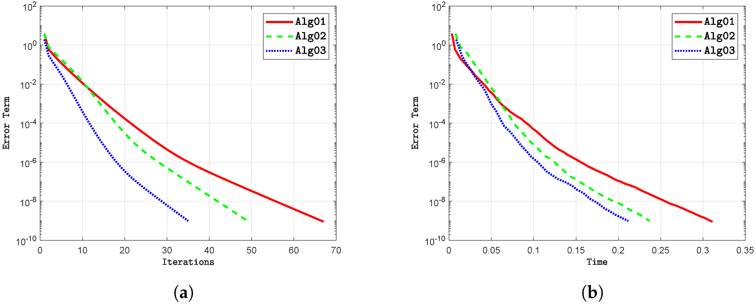
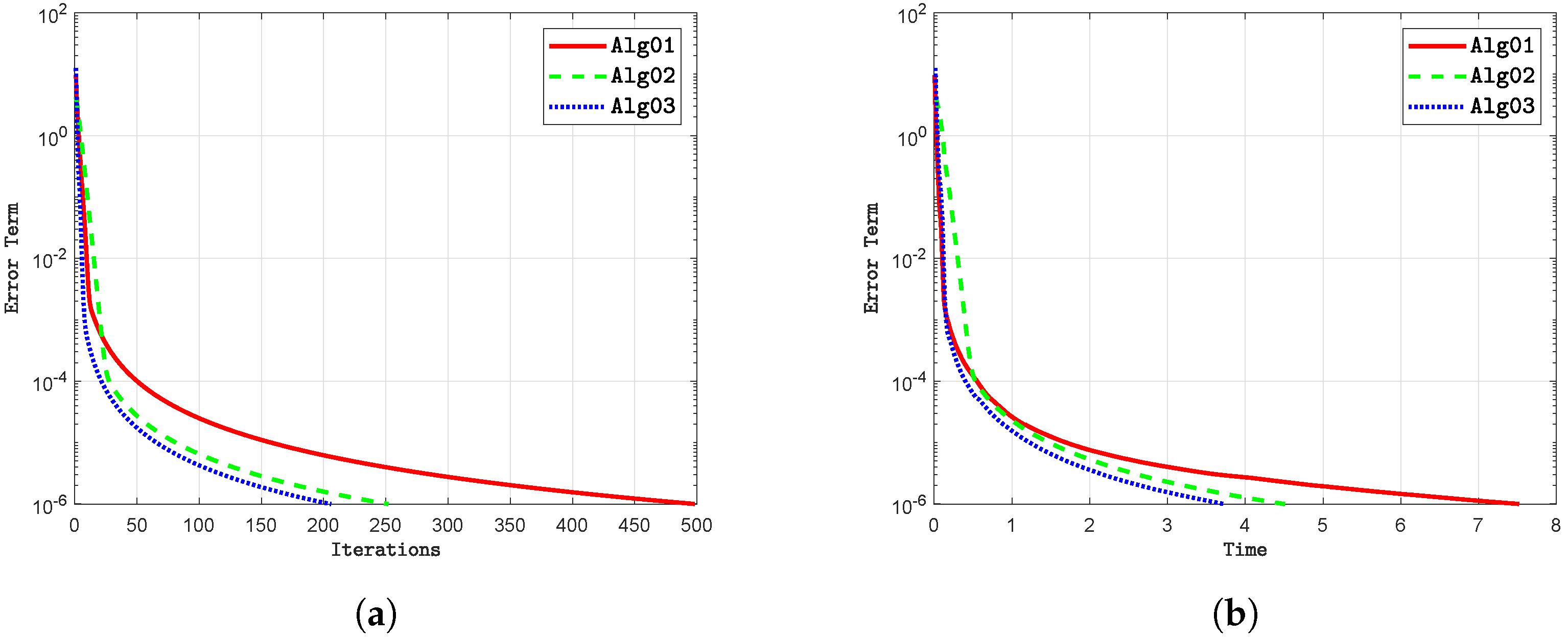
This section demonstrates the effectiveness of the newly proposed low-cost inertial extragradient method through a series of carefully selected numerical examples. These examples underscore the method’s efficient convergence and its capability to address computational challenges in problems related to equilibrium and fixed points under convex constraints. The numerical results affirm that our method represents not only a theoretical advancement but also a practical and adaptable tool, providing valuable insights for researchers in this domain.

All computations were conducted using MATLAB R2018b on a standard HP laptop equipped with an Intel Core i5-6200 processor and 8 GB of RAM. This setup ensures the reproducibility and reliability of the findings within typical research and industry computing environments.

Example 1. 

Consider the HpHard problem, which has been thoroughly investigated in numerical experiments by Harker and Pang [45]. Define the operator $\mathcal{S}:{\mathbb{R}}^m\to {\mathbb{R}}^m$ as $\mathcal{S}\left(u\right)=Mu+q,$ where $q=0$, and

$$M=N{N}^T+B+D.$$

In our numerical experiments, we use a random matrix $N=\mathit{rand}\left(m\right)$, a skew-symmetric matrix defined as $B=0.5K-0.5K^T$, where $K=\mathit{rand}\left(m\right)$, and a diagonal matrix $D=\mathit{diag}\left(\mathit{rand}\right(m,1\left)\right)$. Define the bifunction $\mathcal{L}:\mathcal{X}\times \mathcal{X}\to \mathbb{R}$ as

$$\mathcal{L}(u,y):=⟨\mathcal{S}\left(u\right),y-u⟩,\forall u,y\in \mathcal{X}.$$

The feasible set $\mathcal{X}$ is given by $\mathcal{X}=\{u\in {\mathbb{R}}^m:-10\le u_i\le 10,\forall i\}.$ It is evident that $\mathcal{L}$ is both monotone and Lipschitz continuous, with constants $2c^1=2c^2=\parallel M\parallel$. Additionally, consider the mapping $\mathcal{Q}:\mathcal{Z}\to \mathcal{Z}$ defined by $\mathcal{Q}\left(u\right)={\displaystyle \frac{1}{2}}u$. In our experiments, we initialize with $u_0=u_1=(2,2,\dots ,2)$.

The numerical results for Example 1 are shown in Figure 1, Figure 2, Figure 3 and Figure 4, as well as in Table 1. These results were obtained by varying the dimensions within the Hilbert space $\mathcal{H}$. Upon analyzing the figures and the table, the following observations can be made:

Figure 1. Comparison of algorithms using Example 1 with $m=5$. (a) Total number of iterations executed with $m=5$. (b) Execution time in seconds with $m=5$.

Figure 2. Comparison of algorithms using Example 1 with $m=10$. (a) Total number of iterations executed with $m=10.$ (b) Execution time in seconds with $m=10.$

Figure 3. Comparison of algorithms using Example 1 with $m=50$. (a) Total number of iterations executed with $m=50.$ (b) Execution time in seconds with $m=50.$

Figure 4. Comparison of algorithms using Example 1 with $m=100$. (a) Total number of iterations executed with $m=100.$ (b) Execution time in seconds with $m=100.$

Table 1. The numerical data for Figure 1, Figure 2, Figure 3 and Figure 4.

m	Iterations/Time
	Alg01	Alg02	Alg03
5	67/0.3111841	49/0.2369935	35/0.2117653
10	77/0.6932886	59/0.4885111	48/0.3821908
50	75/0.4502335	59/0.3711017	47/0.2621170
100	68/0.5512957	56/0.6928128	45/0.3807845

i

The variation in dimensions within a real Hilbert space $\mathcal{H}$ has minimal impact on the iteration count across all algorithms. Our proposed algorithm consistently demonstrates a lower iteration count compared to alternative methods in all scenarios. Thus, the dimensionality of the Hilbert space appears to have a negligible influence on the iteration count, regardless of the algorithm employed.

ii

The execution time may vary slightly depending on the dimensions of the Hilbert space $\mathcal{H}$, even when the number of iterations remains constant. Generally, our proposed algorithm tends to complete tasks more quickly, typically measured in seconds, compared to other methods. However, it is challenging to identify a clear trend from these results. Consequently, the choice of dimensions in the Hilbert space seems to have little effect on execution time across all algorithms.

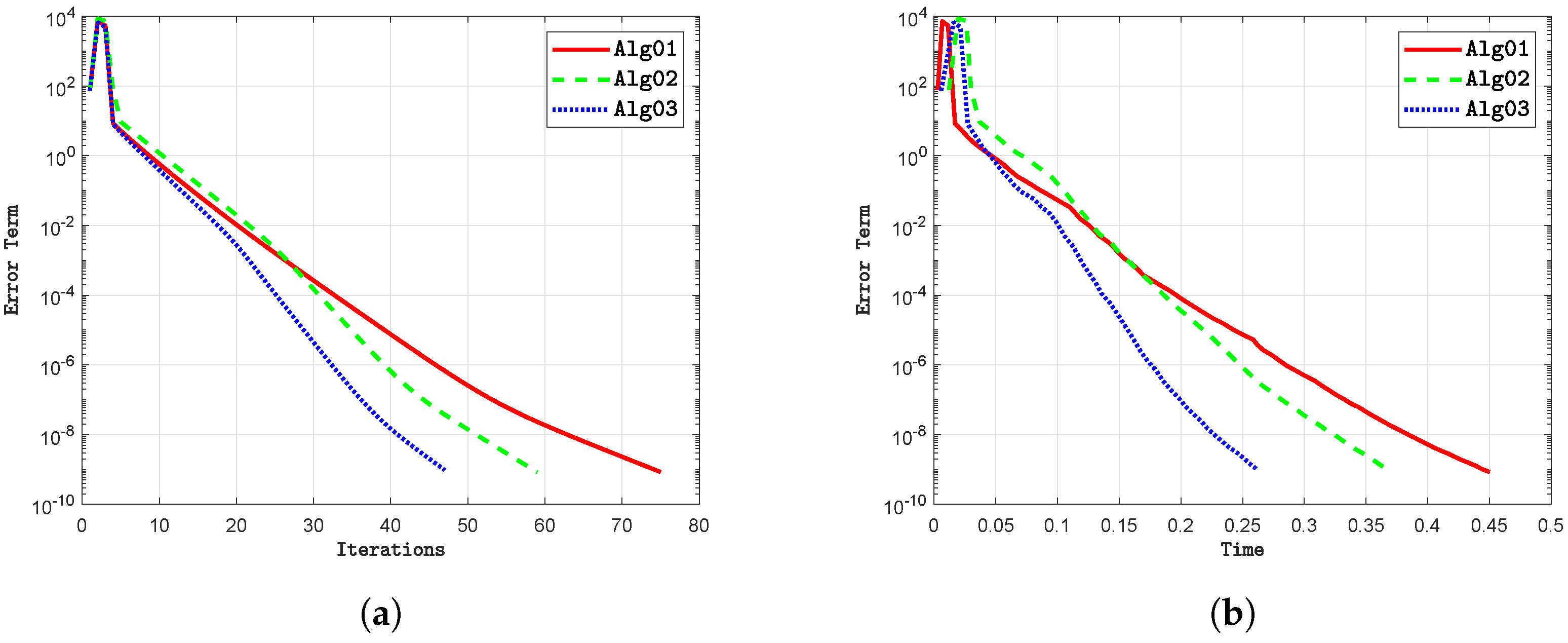
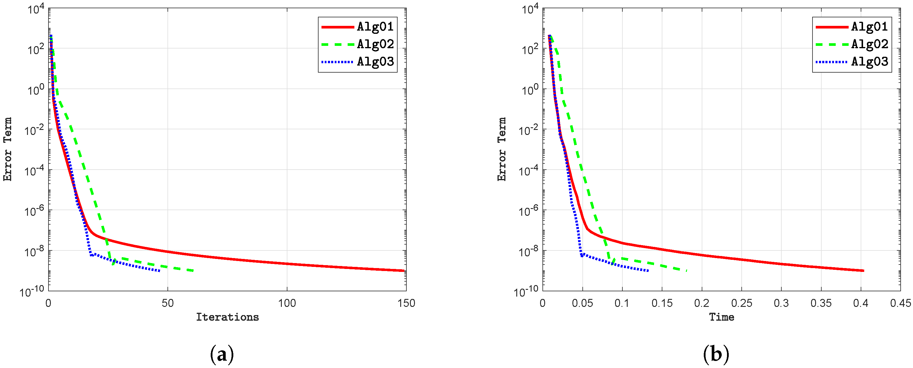
The execution of the algorithms follows specific configurations of control parameters. First, we apply Algorithm 1 from [37], denoted as (Alg01), with the following parameter settings ${\lambda }_n={\displaystyle \frac{1}{4c^1}},{\beta }_n={\displaystyle \frac{1}{2(n+2)}},{\alpha }_n={\displaystyle \frac{1}{2}}.$ Second, we utilize Algorithm 3.1 from [38], referred to as (Alg02), with the following parameter specifications: ${\lambda }_1=0.32,\wp =0.68,\mu =0.56,\delta ={\displaystyle \frac{1}{1+\mu }},{ϵ}_n={\displaystyle \frac{100}{{(1+n)}^2}},{\beta }_n={\displaystyle \frac{1}{2(n+2)}},{\sigma }_n=0.1,\phi \left(x\right)=0.1x.$ Lastly, we implement Algorithm 1, denoted as (Alg03), with the following parameter values ${\lambda }_1=0.32,\wp =0.68,\mu =0.56,{ϵ}_n={\displaystyle \frac{100}{{(1+n)}^2}},{\beta }_n={\displaystyle \frac{1}{2(n+2)}},{\alpha }_n={\displaystyle \frac{1}{2}}.$

Example 2. 

The second problem under consideration arises from the Nash–Cournot Oligopolistic Equilibrium model, as discussed in [17]. Let us consider a function $q:\mathcal{Z}\to \mathbb{R}$ defined as

$${\mathit{lev}}_{\le q}:=\{u\in \mathcal{Z}:q\left(u\right)\le 0\}\ne \varnothing .$$

The subgradient projection is defined by

$$\mathcal{Q}\left(u\right)=\left\{\begin{array}{cc}u-{\displaystyle \frac{q\left(u\right)}{{\parallel r\left(u\right)\parallel }^2}}r\left(u\right),\hfill & \mathit{if}q\left(u\right)\ge 0,\hfill \\ u,\hfill & \mathit{otherwise}.\hfill \end{array}\right.$$

In this context, let $r\left(u\right)\in \partial q\left(u\right)$. As a result, $\mathcal{Q}$ is quasi-nonexpansive, demiclosed at zero, and its fixed point set is given by $\mathit{Fix}\left(\mathcal{Q}\right)={\mathit{lev}}_{\le q}$. Additionally, let us define the bifunction $\mathcal{L}$ as

$$\mathcal{L}(u,y)=⟨Pu+Qy+c,y-u⟩,$$

where $c\in {\mathbb{R}}^m$ and $P,Q$ are $m\times m$ matrices. The matrix $Q-P$ is symmetric and negative semidefinite, whereas P is symmetric and positive semidefinite, with Lipschitz constants $c^1=c^2={\displaystyle \frac{1}{2}}\parallel P-Q\parallel$ (for further details, see [17]).

In the numerical study, the initial points are defined as $u_0=u_1=(2,2,\dots ,2)$. The dimensionality of the space varies, and the stopping condition is established by the error term $\parallel {\nu }_n-y_n\parallel \le {10}^{-6}$. Figure 5, Figure 6, Figure 7 and Figure 8, along with Table 2, show the numerical results from analyzing different dimensions in the Hilbert space $\mathcal{H}$. Upon reviewing these visual representations and the data presented in the table, we can draw the following conclusions:

Figure 5. Comparison of algorithms using Example 2 with $m=5$. (a) Total number of iterations with $m=5.$ (b) Execution time in seconds with $m=5.$

Figure 6. Comparison of algorithms using Example 2 with $m=20$. (a) Total number of iterations with $m=20.$ (b) Execution time in seconds with $m=20.$

Figure 7. Comparison of algorithms using Example 2 with $m=50$. (a) Total number of iterations with $m=50.$ (b) Execution time in seconds with $m=50.$

Figure 8. Comparison of algorithms using Example 2 with $m=100$. (a) Total number of iterations with $m=100.$ (b) Execution time in seconds with $m=100.$

Table 2. The numerical data for Figure 5, Figure 6, Figure 7, Figure 8.

m	Iterations/Time
	Alg01	Alg02	Alg03
5	211/2.33566340	125/1.23511500	102/1.38604810
20	345/6.18899560	175/3.12542860	145/2.63027500
50	498/7.51796940	252/4.50674670	206/3.74000570
100	603/12.1350324	298/4.26217260	220/4.34698240

(i)

The proposed algorithm consistently demonstrates a lower number of iterations compared to alternative methods across different scenarios. It is evident that, regardless of the algorithm employed, the dimensionality of the Hilbert space significantly influences the iteration count. Notably, as the dimensionality increases, the iteration count also increases for all algorithms.

(ii)

The proposed algorithm consistently exhibits shorter execution times, measured in seconds, compared to alternative methods across various scenarios. It is apparent that, irrespective of the algorithm utilized, the dimensionality of the Hilbert space has a significant impact on execution time. Importantly, as the dimensionality increases, execution time also tends to increase for all algorithms.

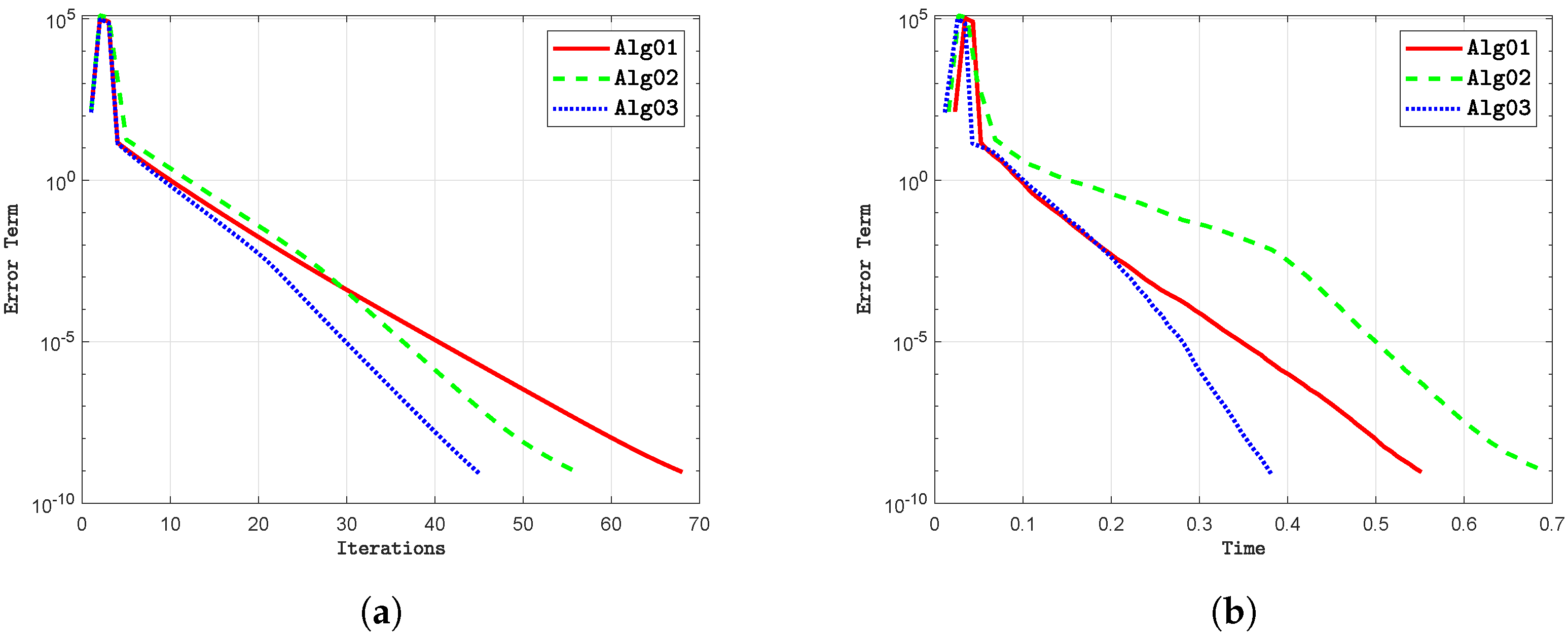
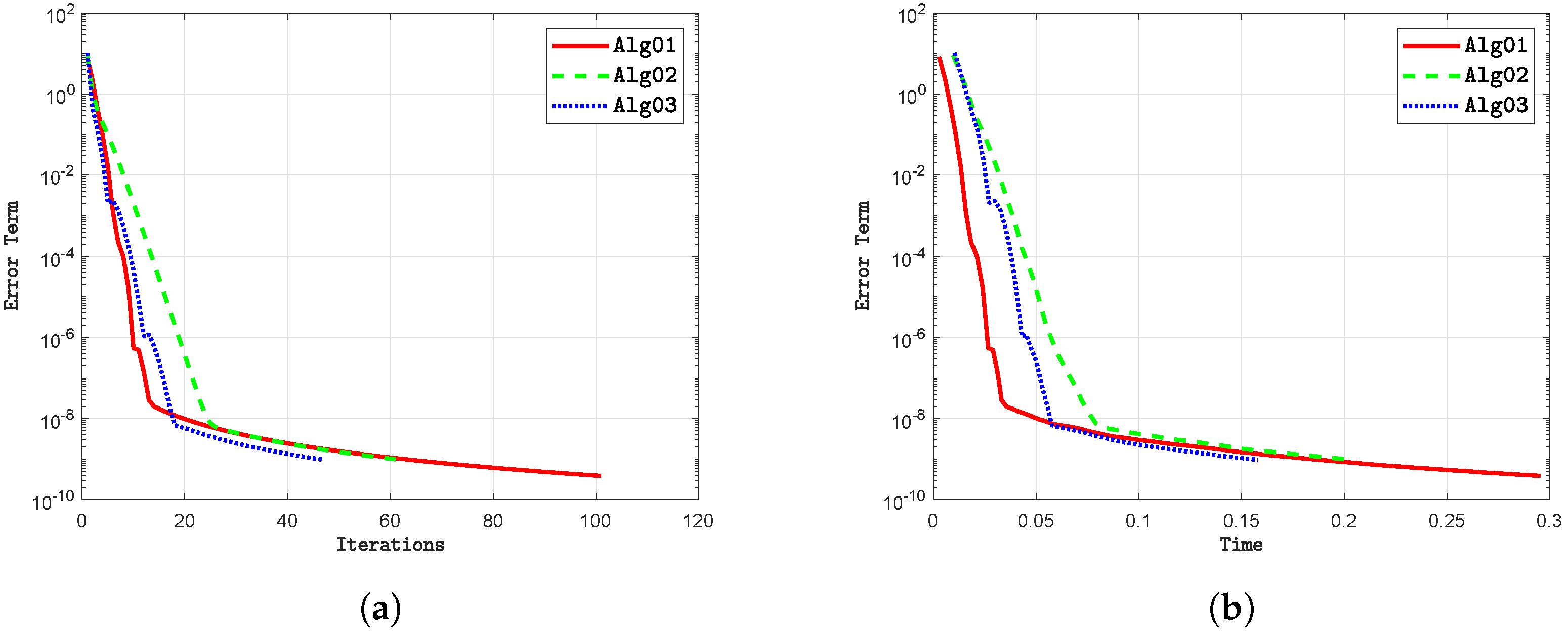
The code is executed using the following control criterion settings. First, we apply Algorithm 1 from [37], denoted as (Alg01), with the parameter values ${\lambda }_n={\displaystyle \frac{1}{4c^1}},{\beta }_n={\displaystyle \frac{1}{2(n+2)}},{\alpha }_n={\displaystyle \frac{1}{2}}.$ Next, we use Algorithm 3.1 from [38], referred to as (Alg02), with the following parameter settings ${\lambda }_1=0.32,\wp =0.68,\mu =0.56,\delta ={\displaystyle \frac{1}{1+\mu }},{ϵ}_n={\displaystyle \frac{100}{{(1+n)}^2}},{\beta }_n={\displaystyle \frac{1}{2(n+2)}},{\sigma }_n=0.1,\phi \left(x\right)=0.1x.$ Finally, we implement Algorithm 1, denoted as (Alg03), with the following parameter values ${\lambda }_1=0.32,\wp =0.68,\mu =0.56,{ϵ}_n={\displaystyle \frac{100}{{(1+n)}^2}},{\beta }_n={\displaystyle \frac{1}{2(n+2)}},{\alpha }_n={\displaystyle \frac{1}{2}}.$

Example 3. 

Let $\mathcal{Z}$ denote the real Hilbert space $L^2\left([0,1]\right)$, with an inner product given by

$$⟨u,y⟩={\int }_0^{1}u\left(p\right)y\left(p\right)dp,\forall u,y\in \mathcal{Z}.$$

The corresponding norm is $\parallel u\parallel =\sqrt{{\int }_0^1{\left|u\left(p\right)\right|}^{2}dp}.$

Let the operator $\mathcal{S}:\mathcal{X}\to \mathcal{Z}$ be defined by

$$\mathcal{S}\left(u\right)\left(p\right)={\int }_0^1\left(u\left(p\right)-H(p,r)\mathit{Fix}\left(u\right(r\left)\right)\right)dr+g\left(p\right),$$

where $\mathcal{X}:=\{u\in L^2\left([0,1]\right):\parallel u\parallel \le 1\}$ represents the unit ball in $\mathcal{X}$, and

$$H(p,r)={\displaystyle \frac{2pr{e}^{(p+r)}}{e\sqrt{e^2-1}}},\mathit{Fix}\left(u\right)=cos\left(u\right),g\left(p\right)={\displaystyle \frac{2p{e}^p}{e\sqrt{e^2-1}}}.$$

Let us define the bifunction as

$$\mathcal{L}(u,y):=⟨\mathcal{S}\left(u\right),y-u⟩,\forall u,y\in \mathcal{X}.$$

The bifunction $\mathcal{L}$ is Lipschitz continuous with constants $c^1=c^2=1$ and satisfies the monotonicity property as described in [46]. The metric projection onto $\mathcal{X}$ is defined as

$$P_{\mathcal{X}}\left(u\right)=\left\{\begin{array}{cc}{\displaystyle \frac{u}{\parallel u\parallel }},\hfill & \mathit{if}\parallel u\parallel >1,\hfill \\ u,\hfill & \mathit{if}\parallel u\parallel \le 1.\hfill \end{array}\right.$$

Now, consider the mapping $\mathcal{Q}:L^2\left([0,1]\right)\to L^2\left([0,1]\right)$ defined by

$$\mathcal{Q}\left(u\right)\left(p\right)={\int }_0^{1}pu\left(r\right)dr,p\in [0,1].$$

A straightforward calculation shows that $\mathcal{Q}$ is 0-demicontractive, with the solution given by $u^{*}\left(p\right)=0$.

Figure 9 and Figure 10 present the numerical results obtained from analyzing two sets of initial points, $u_0$ and $u_1$, selected from the set $\mathcal{X}$. The following observations can be made:

Figure 9. Comparison of algorithms using Example 3: performance evaluation with $u_0=sin\left(p\right).$ (a) Total number of iterations executed with $u_0=sin\left(p\right).$ (b) Execution time in seconds with $u_0=sin\left(p\right).$

Figure 10. Comparison of algorithms using Example 3: performance evaluation with $u_0=cos\left(p\right).$ (a) Total number of iterations executed with $u_0=cos\left(p\right).$ (b) Execution time in seconds with $u_0=cos\left(p\right).$

i

Modifying the initial points $x_0$ and $x_1$ influences the number of iterations required by the algorithms. Our proposed method generally requires fewer iterations compared to existing approaches.

ii

The execution time for each algorithm varies based on the selected initial points; however, our method typically completes in less time than the alternatives.

The algorithms are executed with the specified control criterion settings. Firstly, we implement Algorithm 1 from [37], referred to as (Alg01), with the following parameter settings ${\lambda }_n={\displaystyle \frac{1}{4c^1}},{\beta }_n={\displaystyle \frac{1}{2(n+2)}},{\alpha }_n={\displaystyle \frac{1}{2}}.$ Secondly, we utilize Algorithm 3.1 from [38], denoted as (Alg02), with the following parameter specifications: ${\lambda }_1=0.32,\wp =0.68,\mu =0.56,\delta ={\displaystyle \frac{1}{1+\mu }},{ϵ}_n={\displaystyle \frac{100}{{(1+n)}^2}},{\beta }_n={\displaystyle \frac{1}{2(n+2)}},{\sigma }_n=0.1,\phi \left(x\right)=0.1x.$ Finally, we implement Algorithm 1, referred to as (Alg03), with the following parameter values: ${\lambda }_1=0.32,\wp =0.68,\mu =0.56,{ϵ}_n={\displaystyle \frac{100}{{(1+n)}^2}},{\beta }_n={\displaystyle \frac{1}{2(n+2)}},{\alpha }_n={\displaystyle \frac{1}{2}}.$

5. Conclusions

This paper introduces a new inertial hybrid algorithm designed to address equilibrium and fixed-point problems within real Hilbert spaces. The proposed algorithm improves upon the classical extragradient method by incorporating inertial terms and implementing a self-adaptive stepsize, leading to enhanced convergence speed and computational efficiency. Under appropriate conditions, the algorithm exhibits strong convergence, thereby providing a solid theoretical foundation. The main contributions of this work include the development of an algorithm that integrates inertial momentum with a dynamically adjusted stepsize. This feature makes the method particularly effective in scenarios where Lipschitz constants are not readily available. The algorithm guarantees convergence to a common fixed point under conditions of pseudomonotonicity and other pertinent assumptions, demonstrating its versatility for a variety of equilibrium and fixed-point problems.

Numerical experiments indicate that the proposed method outperforms existing algorithms in terms of convergence rate, accuracy, and robustness, underscoring its practical applicability in optimization, game theory, and variational analysis. Future research may explore extending the algorithm to infinite-dimensional spaces and non-convex problems, as well as applying inertial techniques and adaptive stepsizes to other optimization challenges.

References

- Qin, X.; An, N.T. Smoothing algorithms for computing the projection onto a Minkowski sum of convex sets. Comput. Optim. Appl. 2019, 74, 821–850. [Google Scholar] [CrossRef]
- An, N.T.; Nam, N.M.; Qin, X. Solving k-center problems involving sets based on optimization techniques. J. Glob. Optim. 2019, 76, 189–209. [Google Scholar] [CrossRef]
- Hussien, A.G.; Hassanien, A.E.; Houssein, E.H.; Amin, M.; Azar, A.T. New binary whale optimization algorithm for discrete optimization problems. Eng. Optim. 2019, 52, 945–959. [Google Scholar] [CrossRef]
- Elmorshedy, M.F.; Almakhles, D.; Allam, S.M. Improved performance of linear induction motors based on optimal duty cycle finite-set model predictive thrust control. Heliyon 2024, 10, e34169. [Google Scholar] [CrossRef] [PubMed]
- Banerjee, P.; Roy, S.; Sinha, A.; Hassan, M.M.; Burje, S.; Agrawal, A.; Bairagi, A.K.; Alshathri, S.; El-Shafai, W. MTD-DHJS: Makespan-Optimized Task Scheduling Algorithm for Cloud Computing with Dynamic Computational Time Prediction. IEEE Access 2023, 11, 105578–105618. [Google Scholar] [CrossRef]
- Debnath, P.; Torres, D.F.M.; Cho, Y.J. Advanced Mathematical Analysis and Its Applications; Chapman and Hall/CRC: Boca Raton, FL, USA, 2023. [Google Scholar] [CrossRef]
- Nash, J.F. Equilibrium points in n-person games. Proc. Natl. Acad. Sci. USA 1950, 36, 48–49. [Google Scholar] [CrossRef]
- Long, G.; Liu, S.; Xu, G.; Wong, S.W.; Chen, H.; Xiao, B. A Perforation-Erosion Model for Hydraulic-Fracturing Applications. SPE Prod. Oper. 2018, 33, 770–783. [Google Scholar] [CrossRef]
- Arrow, K.J.; Debreu, G. Existence of an Equilibrium for a Competitive Economy. Econometrica 1954, 22, 265–290. [Google Scholar] [CrossRef]
- Kundur, D.; Hatzinakos, D. Blind image deconvolution. IEEE Signal Process. Mag. 1996, 13, 4–64. [Google Scholar] [CrossRef]
- Patriksson, M. The Traffic Assignment Problem: Models and Methods; Courier Dover Publications: Chicago, IL, USA, 2015. [Google Scholar]
- Nash, J. Non-Cooperative Games. Ann. Math. 1951, 54, 286. [Google Scholar] [CrossRef]
- Fan, K. A Minimax Inequality and Applications. In Inequalities III; Shisha, O., Ed.; Academic Press: New York, NY, USA, 1972. [Google Scholar]
- Nikaidô, H.; Isoda, K. Note on non-cooperative convex game. Pac. J. Math. 1955, 5, 807–815. [Google Scholar] [CrossRef]
- Gwinner, J. On the penalty method for constrained variational inequalities. Optim. Theory Algorithms 1981, 86, 197–211. [Google Scholar]
- Flåm, S.D.; Antipin, A.S. Equilibrium programming using proximal-like algorithms. Math. Program. 1996, 78, 29–41. [Google Scholar] [CrossRef]
- Tran, D.Q.; Dung, M.L.; Nguyen, V.H. Extragradient algorithms extended to equilibrium problems. Optimization 2008, 57, 749–776. [Google Scholar] [CrossRef]
- Korpelevich, G. The extragradient method for finding saddle points and other problems. Matecon 1976, 12, 747–756. [Google Scholar]
- Rehman, H.U.; Kumam, W.; Sombut, K. Inertial modification using self-adaptive subgradient extragradient techniques for equilibrium programming applied to variational inequalities and fixed-point problems. Mathematics 2022, 10, 1751. [Google Scholar] [CrossRef]
- Ceng, L.C.; Yao, J.C. A hybrid iterative scheme for mixed equilibrium problems and fixed point problems. J. Comput. Appl. Math. 2008, 214, 186–201. [Google Scholar] [CrossRef]
- Zeng, L.C.; Yao, J.C. Strong convergence theorem by an extragradient method for fixed point problems and variational inequality problems. Taiwan. J. Math. 2006, 10, 1293–1303. [Google Scholar] [CrossRef]
- Peng, J.W.; Yao, J.C. A new hybrid-extragradient method for generalized mixed equilibrium problems, fixed point problems and variational inequality problems. Taiwan. J. Math. 2008, 12, 1401–1432. [Google Scholar] [CrossRef]
- Kumam, W.; Rehman, H.U.; Kumam, P. A new class of computationally efficient algorithms for solving fixed-point problems and variational inequalities in real Hilbert spaces. J. Inequalities Appl. 2023, 2023, 48. [Google Scholar] [CrossRef]
- Rehman, H.; Kumam, P.; Suleiman, Y.I.; Kumam, W. An adaptive block iterative process for a class of multiple sets split variational inequality problems and common fixed point problems in hilbert spaces. Numer. Algebr. Control Optim. 2023, 13, 273–298. [Google Scholar] [CrossRef]
- Khunpanuk, C.; Panyanak, B.; Pakkaranang, N. A New Construction and Convergence Analysis of Non-Monotonic Iterative Methods for Solving ρ-Demicontractive Fixed Point Problems and Variational Inequalities Involving Pseudomonotone Mapping. Mathematics 2022, 10, 623. [Google Scholar] [CrossRef]
- Anh, P.N. A hybrid extragradient method extended to fixed point problems and equilibrium problems. Optimization 2013, 62, 271–283. [Google Scholar] [CrossRef]
- Vuong, P.T.; Strodiot, J.J.; Nguyen, V.H. Extragradient methods and linesearch algorithms for solving Ky Fan inequalities and fixed point problems. J. Optim. Theory Appl. 2012, 155, 605–627. [Google Scholar] [CrossRef]
- Vuong, P.T.; Strodiot, J.J.; Nguyen, V.H. On extragradient-viscosity methods for solving equilibrium and fixed point problems in a Hilbert space. Optimization 2015, 64, 429–451. [Google Scholar] [CrossRef]
- Takahashi, W.; Wen, C.; Yao, J. The shrinking projection method for a finite family of demimetric mapping with variational inequality problems in a Hilbert space. Fixed Point Theor. 2018, 19, 407–420. [Google Scholar] [CrossRef]
- Dadashi, V.; Iyiola, O.S.; Shehu, Y. The subgradient extragradient method for pseudomonotone equilibrium problems. Optimization 2020, 69, 901–923. [Google Scholar] [CrossRef]
- Hieu, D.V.; Gibali, A. Strong convergence of inertial algorithms for solving equilibrium problems. Optim. Lett. 2020, 14, 1817–1843. [Google Scholar] [CrossRef]
- Hieu, D.V.; Quy, P.K.; Vy, L.V. Explicit iterative algorithms for solving equilibrium problems. Calcolo 2019, 56, 11. [Google Scholar] [CrossRef]
- Shehu, Y.; Iyiola, O.S.; Thong, D.V.; Van, N.T.C. An inertial subgradient extragradient algorithm extended to pseudomonotone equilibrium problems. Math. Meth. Oper. Res. 2021, 93, 213–242. [Google Scholar] [CrossRef]
- Censor, Y.; Gibali, A.; Reich, S. The subgradient extragradient method for solving variational inequalities in Hilbert space. J. Optim. Theory Appl. 2011, 148, 318–335. [Google Scholar] [CrossRef] [PubMed]
- Censor, Y.; Gibali, A.; Reich, S. Strong convergence of subgradient extragradient methods for the variational inequality problem in Hilbert space. Optim. Methods Softw. 2011, 26, 827–845. [Google Scholar] [CrossRef]
- Thong, D.V.; Cholamjiak, P.; Rassias, M.T.; Cho, Y.J. Strong convergence of inertial subgradient extragradient algorithm for solving pseudomonotone equilibrium problems. Optim. Lett. 2021, 73, 1329–1354. [Google Scholar] [CrossRef]
- Hieu, D.V. Strong convergence of a new hybrid algorithm for fixed point problems and equilibrium problems. Math. Model. Anal. 2018, 24, 1–19. [Google Scholar] [CrossRef]
- Tan, B.; Cho, S.Y.; Yao, J.C. Accelerated inertial subgradient extragradient algorithms with non-monotonic stepsizes for equilibrium problems and fixed point problems. J. Nonlinear Var. Anal. 2022, 6, 89–122. [Google Scholar] [CrossRef]
- Bauschke, H.H.; Combettes, P.L. Convex Analysis and Monotone Operator Theory in Hilbert Spaces, 2nd ed.; CMS Books in Mathematics; Springer International Publishing: Berlin/Heidelberg, Germany, 2017. [Google Scholar]
- Bianchi, M.; Schaible, S. Generalized monotone bifunctions and equilibrium problems. J. Optim. Theory Appl. 1996, 90, 31–43. [Google Scholar] [CrossRef]
- Takahashi, W. A general iterative method for split common fixed point problems in Hilbert spaces and applications. Pure Appl. Funct. Anal. 2018, 3, 349–370. [Google Scholar]
- Song, Y. Iterative methods for fixed point problems and generalized split feasibility problems in Banach spaces. J. Nonlinear Sci. Appl. 2018, 11, 198–217. [Google Scholar] [CrossRef]
- Goebel, K.; Kirk, W. Topics in Metric Fixed Point Theory; Cambridge University Press: Cambridge, UK, 1990. [Google Scholar] [CrossRef]
- Saejung, S.; Yotkaew, P. Approximation of zeros of inverse strongly monotone operators in Banach spaces. Nonlinear Anal. Theor. 2012, 75, 742–750. [Google Scholar] [CrossRef]
- Harker, P.T.; Pang, J.S. For the Linear Complementarity Problem; Lectures in Applied Mathematics; Society for Industrial and Applied Mathematics: Philadelphia, PA, USA, 1990; Volume 26. [Google Scholar]
- Hieu, D.V.; Anh, P.K.; Muu, L.D. Modified hybrid projection methods for finding common solutions to variational inequality problems. Comput. Optim. Appl. 2016, 66, 75–96. [Google Scholar] [CrossRef]
Disclaimer/Publisher’s Note: The statements, opinions and data contained in all publications are solely those of the individual author(s) and contributor(s) and not of MDPI and/or the editor(s). MDPI and/or the editor(s) disclaim responsibility for any injury to people or property resulting from any ideas, methods, instructions or products referred to in the content. |
© 2024 by the authors. Licensee MDPI, Basel, Switzerland. This article is an open access article distributed under the terms and conditions of the Creative Commons Attribution (CC BY) license (https://creativecommons.org/licenses/by/4.0/).