Iteratively Reweighted Least Squares Fiducial Interval for Variance in Unbalanced Variance Components Model

Abstract

The objective of this work is to propose the iteratively reweighted least squares concept to form a fiducial generalized pivotal quantity of the between-group variance component for the unbalanced variance components model. The fiducial generalized pivotal quantity is a subclass of the generalized pivotal quantity which is useful technique to deal with problem of nuisance parameters for finding interval estimator. This research provides the probability distribution and the properties of the statistics to lead the constructing of the confidence interval. The authors also prove the construction of the fiducial generalized pivotal quantity through iteratively reweighted least squares. The performance comparison for the new proposed method with other competing methods in the literature is studied through a simulation study. The results of the simulation study demonstrate that the proposed method is very satisfactory in terms of both the coverage probability and the average width of the confidence interval. Furthermore, the analysis of real data for patients of sickle cell disease also illustrates that the proposed method gives the smallest average width of the confidence interval. All these results confirm that the iteratively reweighted least squares fiducial generalized pivotal quantity confidence interval is recommended.

1. Introduction

The variance components model plays a vital role in several fields, such as industrial process management, agricultural genetics, medical treatment, animal breeding studies, etc. The variance components model is also called the random effects model, the conclusions of which can be applied to the entire population level of factors. Consider the variance components model given by

$$\begin{array}{c}\hfill y_{ij}=\mu +a_i+e_{ij},i=1,\dots ,g,j=1,\dots ,n_i,\end{array}$$

(1)

where $y_{ij}$ is the jth random observation associated with the ith group of the random factor, and $\mu$ is the grand mean. The ith group of the random factor, $a_i$, is distributed as $N(0,{\sigma }_a^2)$. The jth random error associated with the ith group of the random factor, $e_{ij}$, is distributed as $N(0,{\sigma }_e^2)$. Both $a_i$ and $e_{ij}$ are mutually independent. It follows that $y_{ij}$ is distributed as $N(\mu ,{\sigma }_a^2+{\sigma }_e^2)$. Here, ${\sigma }_a^2$ and ${\sigma }_e^2$ are known as variance components. Generally, ${\sigma }_a^2$ and ${\sigma }_e^2$ are called the between-group variance and within-group variance, respectively. The number of observations is denoted as $n_i$, $i=1,\dots ,g$ and the overall sample size is denoted as $n={\sum }_{i=1}^g{n}_i$. The model (1) is called a balanced model when $n_i$ of each group is equal. Otherwise, it is called an unbalanced model.

The minimal sufficient statistic is an important property for an estimator, which is used to form the confidence interval about the parameter of interest when the probability distribution for the statistic can be obtained [1]. For the balanced random effects model, the minimal sufficient statistics are available in closed-form expression. Nevertheless, this expression is unavailable for the unbalanced random effects model. Moreover, resolving the closed-form expression for the minimal sufficient statistic is rather complicated in the unbalanced case [2]. In this research, we are concerned with the inference of the between-group variance component for the unbalanced variance components model. There are numerous works from the literature that provide a method to make an inference about the variance component for the unbalanced random model, such as those of Ting et al. [3] in 1990 and Hartung and Knapp [4] in 2000, which are based on an asymptotic frequentist method. The favorite method for making an inference about the parameter of interest is a pivotal quantity approach applied by Wald [5] in 1940, Thomas and Hultquist [6] in 1978 and Park and Burdick [7] in 2003. Alternatively, Li and Li [8] in 2005 utilized the method via a fiducial inference using the concept provided by Fisher [9] in 1935. Later, the connection between the pivotal quantity approach and the fiducial inference was presented by Hannig et al. [10] in 2006. According to this connection, the construction for the series of fiducial generalized confidence interval for variance components was provided by Lidong et al. [11] in 2008, and the fiducial generalized pivotal quantity through the least squares concept for finding confidence interval for the parameters of interest was proposed by Liu et al. [12] in 2015.

There are several works in the literature that construct the confidence intervals of ${\sigma }_a^2$ in an unbalanced random effects model. For instance, Ting et al. [3] in 1990 and Hartung and Knapp [4] in 2000 applied the classical exact method to construct confidence intervals of ${\sigma }_a^2$. In 2003, Park and Burdick [7] presented the closed-form expression for the minimal sufficient statistic in the unbalanced case and used the idea of the generalized pivotal quantity to construct the confidence interval about the parameter of interest. In 2005, Li and Li [8] applied the fiducial approach to derive the confidence interval of the between-group variance component in unbalanced random effects model. Later, Liu et al. [12] in 2015 utilized the concept of the generalized pivotal quantity and the fiducial approach via the least square idea for obtaining confidence interval of variance components in unbalanced two-component normal mixed linear model. The point of this study is to propose a new iteratively reweighted least squares fiducial generalized pivotal quantity to form the confidence intervals of the between-group variance component for the unbalanced variance components model. The methods for comparing the performance with the proposed method are as follows: the TG method [3], the HK method [4], the PB method [7], the LL method [8], and the LXH method [12].

The organization for the remaining of this research is the following: the idea of the fiducial generalized pivotal quantity for finding confidence intervals is introduced in Section 2. The new iterative reweighted least squares fiducial generalized pivotal quantity to construct the confidence interval of ${\sigma }_a^2$ is proposed in Section 3. We perform simulation studies to investigate its performance in Section 4. Section 5 illustrates the application utilizing the new proposed method. A conclusion is presented in Section 6.

2. Review of Fiducial Generalized Pivotal Quantity

The idea of a generalized pivotal quantity is a useful technique to deal with the problem of nuisance parameters for finding interval estimation. The fiducial generalized pivotal quantity (FGPQ) is a subclass of the generalized pivotal quantity, which is based on an extension of the fiducial argument proposed by Fisher [9] in 1935. The FGPQ are extensively used to obtain confidence intervals. For instance, Lidong et al. [11] in 2008 focused on developing fiducial intervals for estimating variance components and intraclass correlation in scenarios with unbalanced data structures. The method of constructing the fiducial intervals was based on an extension of the fiducial approach presented by Fisher [9] in 1935. Moreover, the results of the simulation study showed satisfactory performance in terms of coverage probability and the average width confidence interval. In 2011, Burch [13] investigated confidence intervals for variance components in the unbalanced one-way random effects model under non-normal distribution assumptions. The procedure of developing confidence intervals was constructed by the FGPQ. Later, Liu and Xu [14] in 2015 proposed a new kind of confidence interval for variance components in a one-way random effects model by deriving the combined asymptotic confidence distribution and property of confidence distribution. In addition, the related measures of variance components such as their ratio and intraclass correlation were presented. Herein, the method of Liu and Xu [14] was based on the FGPQ. In 2015, Liu et al. [12] developed the use of least squares for the FGPQ to construct confidence intervals for variance components in a two-component normal mixed linear model. Based on the aforementioned works in the literature, Li and Li [15] in 2007 and Jiratampradab et al. [16] in 2022 compared those methods via the FGPQ for constructing confidence intervals for variance components in an unbalanced one-way random effects model. In this regard, the motivation of this study is to use the FGPQ to obtain the inference about variance components. The definition of the FGPQ derived from Hannig et al. [10] in 2006 is stated below.

Definition 1.

Assume that $\mathbf{S}$ is a vector of observable random such that the distribution of $\mathbf{S}$ is indexed through vector of parameter ξ, where $\mathbf{S}$ and ξ are elements of ${\mathbb{R}}^k$. Suppose that $\theta =\pi \left(\xi \right)$ is a parameter to make inferences, where θ is element of ${\mathbb{R}}^q(q\ge 1)$. An independent copy of $\mathbf{S}$ is represented by ${\mathbf{S}}^{*}$. The realized values of $\mathbf{S}$ and ${\mathbf{S}}^{*}$ are denoted by $\mathbf{s}$ and ${\mathbf{s}}^{*}$, respectively. A fiducial generalized pivotal quantity for θ is denoted by ${\mathcal{R}}_{\theta }(\mathbf{S},{\mathbf{S}}^{*},\xi )$. The properties of ${\mathcal{R}}_{\theta }(\mathbf{S},{\mathbf{S}}^{*},\xi )$ are given as follows:

1. The conditional distribution of ${\mathcal{R}}_{\theta }(\mathbf{S},{\mathbf{S}}^{*},\xi )$ is free of ξ, where $\mathbf{S}=\mathbf{s}$.

2. For all $\mathbf{s}$, which is an element of ${\mathbb{R}}^k$, ${\mathcal{R}}_{\theta }(\mathbf{s},{\mathbf{s}}^{*},\xi )=\theta$.

• The FGPQ for θ is derived from the percentiles of ${\mathcal{R}}_{\theta }(\mathbf{s},{\mathbf{s}}^{*},\xi )$.

3. Confidence Interval for ${\mathit{\sigma }}_{\mathit{a}}^{\mathbf{2}}$

3.1. Matrix Formulation of Model

In order to obtain the matrix formulation, let an $n\times 1$ vector $\mathbf{Y}$ represent the observations, and thus the model (1) can be shown as

$$\begin{array}{cc}\hfill \mathbf{Y}& =\mu {\mathbf{1}}_n+\mathbf{ZA}+\mathbf{E},\hfill \end{array}$$

(2)

where $\mu$ is the grand mean, ${\mathbf{1}}_n$ is an $n\times 1$ vector of ones, $\mathbf{Z}$ is an $n\times g$ incidence matrix, $\mathbf{A}$ is the vector of the random factor with $\mathbf{A}\sim N({\mathbf{0}}_g,{\sigma }_a^2{\mathbf{I}}_g)$, and $\mathbf{E}$ is the vector of the random error with $\mathbf{E}\sim N({\mathbf{0}}_n,{\sigma }_e^2{\mathbf{I}}_n)$. Note that ${\mathbf{0}}_k$ is a $k\times 1$ vector of zero, and ${\mathbf{I}}_k$ is a $k\times k$ identity matrix. Independence among $\mathbf{A}$ and $\mathbf{E}$ is assumed. A horizontal concatenation for matrices ${\mathbf{1}}_n$ and ${\mathbf{ZZ}}^{\prime }$ is denoted as $\mathbf{X}=({\mathbf{1}}_n,{\mathbf{ZZ}}^{\prime })$. Denote $r_1=rank\left(\mathbf{X}\right)-rank\left({\mathbf{1}}_n\right)$ and $r_2=n-rank\left(\mathbf{X}\right)$. The matrix of dimension $n\times (n-1)$, namely, $\mathbf{H}$ is satisfied ${\mathbf{H}}^{\prime }\mathbf{H}={\mathbf{I}}_{n-1}$, where $\mathbf{H}$ is, herein, a Householder matrix. The distribution of $\mathbf{Y}$ in model (2) is given by $\mathbf{Y}\sim N(\mu {\mathbf{1}}_n,{\sigma }_a^2{\mathbf{ZZ}}^{\prime }+{\sigma }_e^2{\mathbf{I}}_n)$, and it follows that

$$\begin{array}{c}\hfill {\mathbf{H}}^{\prime }\mathbf{Y}\sim N({\mathbf{0}}_{n-1},{\sigma }_a^2{\mathbf{H}}^{\prime }{\mathbf{ZZ}}^{\prime }\mathbf{H}+{\sigma }_e^2{\mathbf{I}}_{n-1}).\end{array}$$

(3)

The distinct eigenvalues of ${\mathbf{H}}^{\prime }{\mathbf{ZZ}}^{\prime }\mathbf{H}$ are ${\lambda }_1,{\lambda }_2,\cdots ,{\lambda }_d$ such that ${\lambda }_1>{\lambda }_2>\cdots >{\lambda }_d\ge 0$ having multiplicities $s_1,s_2,\dots ,s_d$. The $(n-1)\times (n-1)$ matrix $\mathbf{P}=[{\mathbf{P}}_1,{\mathbf{P}}_2,\dots ,{\mathbf{P}}_d]$ is orthogonal such that ${\mathbf{P}}^{\prime }{\mathbf{H}}^{\prime }{\mathbf{ZZ}}^{\prime }\mathbf{H}\mathbf{P}=\mathrm{diag}({\lambda }_1{\mathbf{1}}_{s_1}^{\prime },{\lambda }_2{\mathbf{1}}_{s_2}^{\prime },\dots ,{\lambda }_d{\mathbf{1}}_{s_d}^{\prime })$, where ${\mathbf{P}}_{\ell }$, $\ell =1,2,\dots ,d$ is an $(n-1)\times s_{\ell }$ corresponding to ${\lambda }_{\ell }$. The independently quadratic forms, defined by

$$\begin{array}{c}\hfill T_{\ell }={\mathbf{Y}}^{\prime }\mathbf{H}{\mathbf{P}}_{\ell }{\mathbf{P}}_{\ell }^{\prime }{\mathbf{H}}^{\prime }\mathbf{Y},\ell =1,2,\dots ,d,\end{array}$$

(4)

are minimal sufficient statistics for ${\sigma }_a^2$. Let $U_{\ell }$, $\ell =1,2,\dots ,d$ be mutually independent. The distribution of $U_{\ell }$ can be written in terms of $T_{\ell },{\sigma }_a^2$ and ${\sigma }_e^2$ as

$$\begin{array}{c}\hfill U_{\ell }={\displaystyle \frac{T_{\ell }}{{\lambda }_{\ell }{\sigma }_a^2+{\sigma }_e^2}}\sim {\chi }_{s_{\ell }}^2,\ell =1,2,\dots ,d,\end{array}$$

(5)

where ${\chi }_{s_{\ell }}^2$ represents the central chi-squared distribution with $s_{\ell }$ degrees of freedom.

3.2. Construction of Iteratively Reweighted Least Squares FGPQ

At first, we construct FGPQ for ${\sigma }_a^2$ using each $T_{\ell },\ell =1,2,\dots ,d$, and $T_{d+1}$. Notice that (5) is a pivotal quantity for ${\sigma }_a^2$. Regarding the sum of squares due to within groups, ${\displaystyle \frac{T_{d+1}}{{\sigma }_e^2}}$ follows the chi-squared distribution with $r_2$ degrees of freedom. According to (4), the minimal sufficient statistics are $(T_{\ell },T_{d+1})$, $\ell =1,2,\dots ,d$. There is an invertible relationship between $(T_{\ell },T_{d+1})$ and $({\sigma }_a^2,{\sigma }_e^2)$. Thus, it is straightforward to provide fiducial inference as described by Hannig et al. [10] in 2006. According to (5), it can be written as

$$T_1=({\lambda }_1{\sigma }_a^2+{\sigma }_e^2)U_1,$$

$$T_2=({\lambda }_2{\sigma }_a^2+{\sigma }_e^2)U_2,$$

(6)

⋮

$$T_d=({\lambda }_d{\sigma }_a^2+{\sigma }_e^2)U_d.$$

Note that (6) represents the structure of the vector of the observable random $\mathbf{T}=(T_1,T_2,\dots ,T_d)$ in term of a random vector $\mathbf{U}=(U_1,U_2,\dots ,U_d)$. The FGPQ for ${\sigma }_a^2$ can be derived by solving a set of equations with the method of the iteratively reweighted least squares. The sum of squares of the differences between $T_{\ell }$ and $({\lambda }_{\ell }{\sigma }_a^2+{\sigma }_e^2)U_{\ell }$ in (6) with the weights can be expressed as

$$\begin{array}{c}\hfill {\displaystyle D=\sum _{\ell =1}^d{w}_{\ell }{[T_{\ell }-({\lambda }_{\ell }{\sigma }_a^2+{\sigma }_e^2)U_{\ell }]}^2,}\end{array}$$

(7)

where $w_{\ell }={|T_{\ell }-({\lambda }_{\ell }{\sigma }_a^2+{\sigma }_e^2)U_{\ell }|}^{-1}$, $\ell =1,2,\dots ,d$. The weighted least squares solution of ${\sigma }_a^2$, represented by ${\widehat{\sigma }}_a^2$, is formed as in Algorithm 1 with the sequence of weights $w_{\ell }^{\left(j\right)}$, $\ell =1,2,\dots ,d$, $j=0,1,2,\dots$. For a complete iterative procedure, we start with the initial value of ${\sigma }_a^2$ as the ordinary least squares solution. The iterations of the reweighted least squares solution continue until the stopping criterion is satisfied, which is specified at 0.001 [17].

Algorithm 1 The weighted least squares solution of ${\sigma }_a^2$

Input: ${\lambda }_{\ell },s_{\ell },$$T_{\ell }$ and $U_{\ell }\sim {\chi }_{s_{\ell }}^2$, $\ell =1,2,\dots ,d$ in (5) for given $\mathbf{Y},{\mathbf{1}}_n$ and $\mathbf{Z}$ in (2).

Output: ${\widehat{\sigma }}_a^2$

1: Initial: ${\widehat{\sigma }}_a^{2\left(0\right)}={\displaystyle \frac{{\displaystyle \sum _{\ell =1}^d{\lambda }_{\ell }{T}_{\ell }{U}_{\ell }-{\sigma }_e^2\sum _{\ell =1}^d{\lambda }_{\ell }{U}_{\ell }^2}}{{\displaystyle \sum _{\ell =1}^d{\lambda }_{\ell }^2{U}_{\ell }^2}}}$.

2: Repeat:

3:        Update: $w_{\ell }^{j-1}={|T_{\ell }-({\lambda }_{\ell }{\widehat{\sigma }}_a^{2(j-1)}+{\sigma }_e^2)U_{\ell }|}^{-1}$, $\ell =1,2,\dots ,d$.

4:        Update: ${\widehat{\sigma }}_a^{2\left(j\right)}$ by minimizing ${\displaystyle \sum _{\ell =1}^d{w}_{\ell }^{j-1}{[T_{\ell }-({\lambda }_{\ell }{\widehat{\sigma }}_a^{2\left(j\right)}+{\sigma }_e^2)U_{\ell }]}^2}$ respect to ${\widehat{\sigma }}_a^{2\left(j\right)}$.

5: Until Convergence $|{\widehat{\sigma }}_a^{2\left(j\right)}-{\widehat{\sigma }}_a^{2(j-1)}| \le 0.001$.

6: Return ${\widehat{\sigma }}_a^2={\widehat{\sigma }}_a^{2\left(j\right)}$.

Next, we define the FGPQ for ${\sigma }_a^2$ given by

$$\begin{array}{c}\hfill {\mathcal{R}}_{{\sigma }_a^2}={\displaystyle \frac{{\displaystyle \sum _{\ell =1}^d{w}_{\ell }{\lambda }_{\ell }{T}_{\ell }{U}_{\ell }^{*}-{\sigma }_e^2\sum _{\ell =1}^d{w}_{\ell }{\lambda }_{\ell }{U}_{\ell }^{{*}^2}}}{{\displaystyle \sum _{\ell =1}^d{w}_{\ell }{\lambda }_{\ell }^2{U}_{\ell }^{{*}^2}}}},\end{array}$$

(8)

where $w_{\ell }={|T_{\ell }-({\lambda }_{\ell }{\sigma }_a^{2(j-1)}+{\sigma }_e^2)U_{\ell }|}^{-1}$, ${\lambda }_{\ell }$ is an eigenvalue of ${\mathbf{H}}^{\prime }{\mathbf{ZZ}}^{\prime }\mathbf{H}$ in (3), $T_{\ell }$ is observable, and $U_{\ell }^{*}$ is the independent copies of $U_{\ell }$ in (5), $\ell =1,2,\dots ,d$. Regarding (8), it can be constructed through the iteratively reweighted least squares as proven in Theorem 1.

Theorem 1.

The FGPQ for ${\sigma }_a^2$ is ${\mathcal{R}}_{{\sigma }_a^2}$ in (8).

Proof. 

The value of ${\sigma }_a^2$ that minimizes D can be obtained by the derivative of (7) with respect to ${\sigma }_a^2$ and equating to zero so that the weighted least squares solution of ${\sigma }_a^2$ is given by

$$\begin{array}{c}\hfill \widehat{{\sigma }_a^2}={\displaystyle \frac{{\displaystyle \sum _{\ell =1}^d{w}_{\ell }{\lambda }_{\ell }{T}_{\ell }{U}_{\ell }-{\sigma }_e^2\sum _{\ell =1}^d{w}_{\ell }{\lambda }_{\ell }{U}_{\ell }^2}}{{\displaystyle \sum _{\ell =1}^d{w}_{\ell }{\lambda }_{\ell }^2{U}_{\ell }^2}}}.\end{array}$$

Let $T_{\ell }^{*}$ be the independent copies of $T_{\ell }$. Notice that $U_{\ell }^{*}={\displaystyle \frac{T_{\ell }^{*}}{{\lambda }_{\ell }{\sigma }_a^2+{\sigma }_e^2}}\sim {\chi }_{s_{\ell }}^2$, $\ell =1,2,\dots ,d$, and we obtain

$$\begin{array}{c}\hfill {\mathcal{R}}_{{\sigma }_a^2}={\displaystyle \frac{{\displaystyle \sum _{\ell =1}^d{w}_{\ell }{\lambda }_{\ell }{T}_{\ell }\frac{T_{\ell }^{*}}{{\lambda }_{\ell }{\sigma }_a^2+{\sigma }_e^2}-{\sigma }_e^2\sum _{\ell =1}^d{w}_{\ell }{\lambda }_{\ell }{\left(\frac{T_{\ell }^{*}}{{\lambda }_{\ell }{\sigma }_a^2+{\sigma }_e^2}\right)}^2}}{{\displaystyle \sum _{\ell =1}^d{w}_{\ell }{\lambda }_{\ell }^2{\left(\frac{T_{\ell }^{*}}{{\lambda }_{\ell }{\sigma }_a^2+{\sigma }_e^2}\right)}^2}}}.\end{array}$$

The distribution of ${\mathcal{R}}_{{\sigma }_a^2}$ is independent of ${\sigma }_a^2$. When $T_{\ell }^{*}=T_{\ell }$ for $\ell =1,2,\dots ,d$, it is proved that ${\mathcal{R}}_{{\sigma }_a^2}={\widehat{\sigma }}_a^2$, so the requirements of Definition 1 are satisfied. □

3.3. Iteratively Reweighted Least Squares Fiducial Generalized Confidence Intervals for ${\sigma }_a^2$

According to Theorem 1, the FGPQ is denoted by ${\mathcal{R}}_{{\sigma }_a^2}$ as the solution of ${\sigma }_a^2$. Then, the iteratively reweighted least squares fiducial generalized confidence intervals of ${\sigma }_a^2$ can be obtained by ${\mathcal{R}}_{{\sigma }_a^2}$. The $(1-\alpha )100\%$ confidence interval of the between-group variance component (${\sigma }_a^2$) is given by

$$\begin{array}{c}\hfill [\max (0,{\left({\mathcal{R}}_{{\sigma }_a^2}\right)}_{{\displaystyle \frac{\alpha }{2}}}),\max (0,{\left({\mathcal{R}}_{{\sigma }_a^2}\right)}_{1-{\displaystyle \frac{\alpha }{2}}})],\end{array}$$

where ${\left({\mathcal{R}}_{{\sigma }_a^2}\right)}_{{\displaystyle \frac{\alpha }{2}}}$ and ${\left({\mathcal{R}}_{{\sigma }_a^2}\right)}_{1-{\displaystyle \frac{\alpha }{2}}}$ are the ${\displaystyle \frac{\alpha }{2}}$ and $1-{\displaystyle \frac{\alpha }{2}}$ quantiles for the distribution of ${\mathcal{R}}_{{\sigma }_a^2}$ in (8), respectively. Denote the solutions of ${\left({\mathcal{R}}_{{\sigma }_a^2}\right)}_{{\displaystyle \frac{\alpha }{2}}}$ and ${\left({\mathcal{R}}_{{\sigma }_a^2}\right)}_{1-{\displaystyle \frac{\alpha }{2}}}$, which are based on the pivotal quantity.

4. Simulation Study

The comparison of the performance for the new proposed method with the previously existing methods is studied through the simulated data. Without loss of generality, the value of $\mu$ in model (2) is set to zero. The values selected for $({\sigma }_a^2,{\sigma }_e^2)$ are $(0.001,0.999),$ $(0.1,0.9),$ $(0.2,0.8),$ $(0.3,0.7),$ $(0.4,0.6),$ $(0.5,0.5),$ $(0.6,0.4),$ $(0.7,0.3),$ $(0.8,0.2),$ $(0.9,0.1),$ and $(0.999,0.001)$. That is, it is defined in the way that $\rho ={\displaystyle \frac{{\sigma }_a^2}{{\sigma }_a^2+{\sigma }_e^2}}$ varies from small to large in the interval $[0.001,0.999]$. The nominal level is set at $0.95$. This process is generated 5000 times for each setting of the values of $({\sigma }_a^2,{\sigma }_e^2)$ and sample size. For the efficiency criterion, the coverage probability and the average width of the confidence interval are considered. Generally, we first consider the coverage probability that maintains at the nominal level, and then the average widths of the confidence interval are compared. The best method gives the smallest average width of the confidence interval. The function of subclass frequencies which is based on the design in the experiment, denoted by $\Phi ={\displaystyle \frac{\tilde{n}g}{{\sum }_{i=1}^g{n}_i}}$, is called the measurements of the imbalanced, where $\tilde{n}={\displaystyle \frac{g}{{\sum }_{i=1}^g\frac{1}{n_i}}}$, where g is the number of groups and $n_i$ is the number of observations of each group [18]. Note that $\Phi$ is the ratio between the harmonic mean and the mean of $(n_1,n_2,\dots ,n_g)$; it follows that $0<\Phi \le 1$ [19]. Moreover, when $\Phi$ is equal to 1, then the model is balanced, and when $\Phi$ is close to 0, then the model is very unbalanced. Table 1 presents eight different cases of unbalanced design for simulation.

Table 1. Cases of unbalanced design for simulation.

Case	$\mathbf{\Phi }$	g	${\mathit{n}}_{\mathit{i}}$
1	$0.044$	3	1    1  100
2	$0.570$	3	3    7   20
3	$0.818$	3	5   10   15
4	$0.556$	4	4    4    20    20
5	$0.807$	4	2    2    4    6
6	$0.410$	5	4    4     4    8   48
7	$0.068$	6	1    1     1    1    1    100
8	$0.935$	6	4    5     5    5    8    8

The simulation study results are illustrated in Figure 1 and Figure 2. The results in Figure 1 present the coverage probability of the confidence interval for ${\sigma }_a^2$. The results in Figure 2 demonstrate the relative difference of the average width of the confidence interval for ${\sigma }_a^2$. The relative width is used to compare the average widths of the confidence interval of the competing method. This relative width is denoted by ${\displaystyle \frac{W_{\mathrm{M}}-W_{\mathrm{IRLF}}}{W_{\mathrm{IRLF}}}}$, where $W_{\mathrm{M}}$ is the average width of the confidence interval of competing methods and $W_{\mathrm{IRLF}}$ is the average width of the confidence interval of the IRLF method [20]. If the value of the relative width is positive, then it indicates that $W_{\mathrm{IRLF}}$ is smaller than $W_{\mathrm{M}}$. On the other hand, if the value of the relative width is negative, then it indicates that $W_{\mathrm{M}}$ is smaller than $W_{\mathrm{IRLF}}$. Furthermore, the relative width equal to zero indicates that $W_{\mathrm{M}}$ is equal to $W_{\mathrm{IRLF}}$.

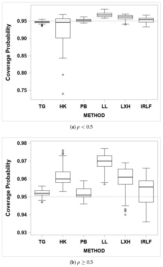
Figure 1. The coverage probability of the 95% confidence interval for ${\sigma }_a^2$.

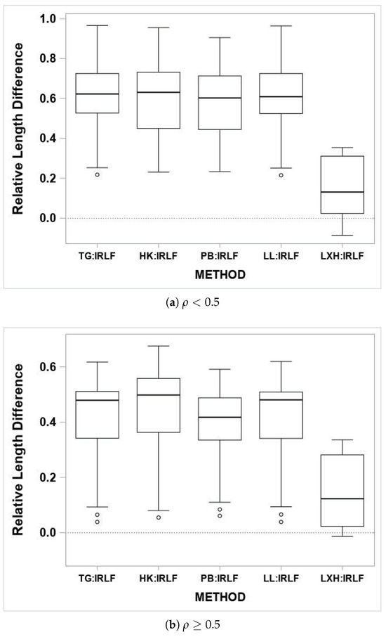
Figure 2. Relative difference of the average width of the 95% confidence interval for ${\sigma }_a^2$.

Figure 1 displays the coverage probability for all competing methods with $\rho <0.5$ and $\rho \ge 0.5$. The TG, PB, and IRLF methods maintain the nominal level, where $\rho <0.5$, and they obtain higher than the nominal level where $\rho \ge 0.5$. The HK method obtains lower than the nominal level where $\rho <0.5$, and it obtains higher than the nominal level where $\rho \ge 0.5$. The LL and LXH methods obtain higher than the nominal level for all situations.

The comparison of the average width of the confidence interval is shown in Figure 2, it implies that the average width of the IRLF interval is the smallest. The average width of the LXH interval is smaller than that of the other four methods. The average widths of the TG, HK, PB and LL intervals behave similarly.

5. Application

The data from Anionwu et al. [21] in 1981 are of a study of the steady-state hemoglobin levels for patients with various types of sickle cell disease. An interesting question is whether steady-state hemoglobin levels differ significantly between patients with the three different types. The three different types are Hemoglobin SS (HbSS), Hemoglobin S-beta-thalassaemia (HbSβ-thal), and Hemoglobin SC (HbSC). The data are shown in Table 2 [22].

Table 2. The steady-state hemoglobin levels in each type of sickle cell disease.

Type	Observations
HbSS	7.2	7.7	8	8.1	8.3	8.4	8.4	8.5	8.6	8.7	9.1	9.1
	9.1	9.8	10.1	10.3
HbSβ-thal	8.1	9.2	10	10.4	10.6	10.9	11.1	11.9	12	12.1
HbSC	10.7	11.3	11.5	11.6	11.7	11.8	12	12.1	12.3	12.6	12.6	13.3
	13.3	13.8	13.9

Model (1) is used to analyze the experiment of the steady-state hemoglobin levels, that is,

$$\begin{array}{c}\hfill y_{ij}=\mu +a_i+e_{ij},i=1,\dots ,g,j=1,\dots ,n_i,\end{array}$$

(9)

where $g=3$, $n_i=(16,10,15)$, $n={\sum }_{i=1}^3{n}_i=41$ and the measurement of the imbalanced is $\Phi =0.958$. Here, $a_i$ denotes the random factor of types of sickle cell disease, and we assume that $a_i$ is normally distributed with a mean of 0 and variance of ${\sigma }_a^2$. $e_{ij}$ represents the jth random error associated with the ith type of sickle cell disease, and we assume that $e_{ij}$ is normally distributed with a mean of 0 and variance of ${\sigma }_e^2$. The independence of $a_i$ and $e_{ij}$ is also assumed. According to Model (2), the vector of the random factor and the vector of the random error are denoted by $\mathbf{A}$ and $\mathbf{E}$, respectively. The distributions of $\mathbf{A}$ and $\mathbf{E}$ are given by $\mathbf{A}\sim N({\mathbf{0}}_3,{\sigma }_a^2{\mathbf{I}}_3)$ and $\mathbf{E}\sim N({\mathbf{0}}_{41},{\sigma }_e^2{\mathbf{I}}_{41})$, respectively. Moreover, $\mathbf{A}$ and $\mathbf{E}$ are independent. Next, we provide the confidence intervals of ${\sigma }_a^2$ followed by the procedure of the proposed method and the previous methods in the literature. The six confidence intervals of ${\sigma }_a^2$ based on the TG, HK, PB, LL, LXH and IRLF methods are demonstrated in Table 3. It is notably seen that the proposed method provides the shortest confidence interval for between-group variance, ${\sigma }_a^2$.

Table 3. The 95% confidence interval of ${\sigma }_a^2$ for the steady-state hemoglobin levels data.

Method	TG	HK	PB	LL	LXH	IRLF
Confidence interval	(0, 126.4)	(0, 127.1)	(0, 116.8)	(0, 135)	(0, 112.4)	(0, 83)

6. Conclusions

This paper proposes a new method to form the confidence interval of between-group variance in the unbalanced variance components model applying the iteratively reweighted least squares concept combining with fiducial generalized pivotal quantity. The simulation study is performed to collate the newly proposed method with five other methods. The results show that the TG, PB, and IRLF methods mostly maintain the nominal level where $\rho$ is small. The HK method is liberal where $\rho$ is small. Conversely, where $\rho$ is large, the HK method is conservative. The LL method is conservative for all situations. The LXH method is mostly conservative for all $\rho$. Clearly, the average width of the IRLF interval is the smallest. Other intervals behave similarly in term of the average width. In summary, these results confirms that the iteratively reweighted least squares fiducial generalized pivotal quantity to form the confidence intervals can be applied instead of the previous methods in the literature. Future research could incorporate the enhanced Laplace approximation [23] to construct the confidence interval for the between-group variance in unbalanced variance components model. Also, it can be used to implement hypothesis tests about the parameters of interest. Additionally, the analysis of the dataset further highlights the satisfactory performance of the IRLF method in terms of the smallest confidence interval. This finding confirms that the confidence interval based on the IRLF method is recommended for practical use in applications in various fields, such as industrial process management [24], animal breeding studies [25], education [26], and so on.

References

- Wackerly, D.; Mendenhall, W.; Scheaffer, R.B. Mathematical Statistics with Applications, 7th ed.; Thomson Learning: Chicago, IL, USA, 2008; p. 468. [Google Scholar]
- Searle, S.R.; Casella, G.; McCulloch, C.E.B. Variance Components; John Wiley and Sons: Hoboken, NJ, USA, 2006; p. 38. [Google Scholar]
- Ting, N.; Burdick, R.K.; Graybill, F.A.; Jeyaratnam, S.; Lu, T.F.C. Confidence intervals on linear combinations of variance components that are unrestricted in sign. J. Stat. Comput. Simul. 1990, 35, 135–143. [Google Scholar] [CrossRef]
- Hartung, J.; Knapp, G. Confidence intervals for the between group variance in the unbalanced one-way random effects model of analysis of variance. J. Stat. Comput. Simul. 2000, 65, 311–323. [Google Scholar] [CrossRef]
- Wald, A. A note on the analysis of variance with unequal class frequencies. Ann. Math. Stat. 1940, 11, 96–100. [Google Scholar] [CrossRef]
- Thomas, J.D.; Hultquist, R.A. Interval estimation for the unbalanced case of the one-way random effects model. Ann. Stat. 1978, 6, 582–587. [Google Scholar] [CrossRef]
- Park, D.J.; Burdick, R.K. Performance of confidence intervals in regression models with unbalanced one-fold nested error structures. Commun. Stat.-Simul. Comput. 2003, 32, 717–732. [Google Scholar] [CrossRef]
- Li, X.; Li, G. Confidence intervals on sum of variance components with unbalanced designs. Commun. Stat.-Theory Methods 2005, 34, 833–845. [Google Scholar] [CrossRef]
- Fisher, R.A. The fiducial argument in statistical inference. Ann. Eugen. 1935, 6, 391–398. [Google Scholar] [CrossRef]
- Hannig, J.; Iyer, H.; Patterson, P. Fiducial generalized confidence intervals. J. Am. Stat. Assoc. 2006, 101, 254–269. [Google Scholar] [CrossRef]
- Lidong, E.; Hannig, J.; Iyer, H. Fiducial intervals for variance components in an unbalanced two-component normal mixed linear model. J. Am. Stat. Assoc. 2008, 103, 854–865. [Google Scholar]
- Liu, X.; Xu, X.; Hannig, J. Least squares generalized inferences in unbalanced two component normal mixed linear model. Comput. Stat. 2015, 31, 973–988. [Google Scholar] [CrossRef]
- Burch, B.D. Confidence intervals for variance components in unbalanced one-way random effects model using non-normal distributions. J. Stat. Plan. Inference 2011, 141, 3793–3807. [Google Scholar] [CrossRef]
- Liu, X.; Xu, X. Confidence distribution inferences in one-way random effects model. Test 2015, 25, 59–74. [Google Scholar] [CrossRef]
- Li, X.; Li, G. Comparison of confidence intervals on the among group variance in the unbalanced variance component model. J. Stat. Comput. Simul. 2007, 77, 477–486. [Google Scholar] [CrossRef]
- Jiratampradab, A.; Supapakorn, T.; Suntornchost, J. Comparison of confidence intervals for variance components in an unbalanced one-way random effects model. Stat. Transit. New Ser. 2022, 23, 149–160. [Google Scholar] [CrossRef]
- Seber, G.A.; Wild, C.J.B. Nonlinear Regression; John Wiley and Sons: Hoboken, NJ, USA, 2003; pp. 582–587. [Google Scholar]
- Ahrens, H.; Pincus, R. On two measures of unbalancedness in a one-way model and their relation to efficiency. Biom. J. 1981, 23, 227–235. [Google Scholar] [CrossRef]
- Khuri, A.I. Measures of imbalance for unbalanced models. Biom. J. 1987, 29, 383–396. [Google Scholar] [CrossRef]
- Tornqvist, L.; Vartia, P.; Vartia, Y.O. How should relative changes be measured? Am. Stat. 1985, 39, 43–46. [Google Scholar]
- Anionwu, E.; Walford, D.; Brozovic, M.; Kirkwood, B. Sickle-cell disease in a British urban community. Br. Med J. 1981, 282, 283–286. [Google Scholar] [CrossRef]
- Sahai, H.; Ageel, M.I. The Analysis of Variance: Fixed, Random and Mixed Models; Springer Science and Business Media: New York, NY, USA, 2000; p. 121. [Google Scholar]
- Han, J.; Lee, Y. Enhanced laplace approximation. J. Multivar. Anal. 2024, 202, 105321. [Google Scholar] [CrossRef]
- Montgomery, D.C. Design and Analysis of Experiments; John Wiley and Sons: Hoboken, NJ, USA, 2017; pp. 133–135. [Google Scholar]
- Sahai, H.; Ojeda, M.M. Analysis of Variance for Random Models, Volume 2: Unbalanced Data: Theory, Methods, Applications, and Data Analysis; Springer Science and Business Media: Boston, UK, 2004; pp. 154–155. [Google Scholar]
- Heiberger, R.M.; Holland, B. Statistical Analysis and Data Display an Intermediate Course with Examples in R; Springer: New York, NY, USA, 2015; p. 215. [Google Scholar]
Disclaimer/Publisher’s Note: The statements, opinions and data contained in all publications are solely those of the individual author(s) and contributor(s) and not of MDPI and/or the editor(s). MDPI and/or the editor(s) disclaim responsibility for any injury to people or property resulting from any ideas, methods, instructions or products referred to in the content. |
© 2025 by the authors. Licensee MDPI, Basel, Switzerland. This article is an open access article distributed under the terms and conditions of the Creative Commons Attribution (CC BY) license (https://creativecommons.org/licenses/by/4.0/).