Evaluation of the Waiting Time in a Finite Capacity Queue with Bursty Input and a Generalized Push-Out Strategy

Abstract

In this paper, we study a finite capacity queue where the arrival process is a special case of the discrete time Markov modulated Poisson process, the service times are generally distributed, and the server takes repeated vacations when the system is empty. The buffer acceptance strategy is based on a generalized push-out scheme: when the buffer is full, an arriving customer pushes out the $N^{th}$ customer in the queue, where $N$ takes values between 2 and the capacity of the system, and the arriving customer joins the end of the queue. Such a strategy is important when, as well as short waiting times for served customers, the time a pushed-out customer occupies a buffer space is also an important performance measure. The Laplace transform of the waiting time of a served customer is determined. Numerical examples show the influence of the bustiness of the input process and also the trade-off between the average waiting time of served customers and the occupancy of the buffer space of pushed-out customers.

1. Introduction

This paper considers a queue with a finite buffer, where the server takes repeated vacations. Customers arrive at the system according to a bursty arrival process. They are served according to a first-come-first-served scheduling scheme. Arriving customers are admitted to the system using a general push-out strategy. When a customer arrives at a full buffer, then the customer in the queue on the $N$th place ($N$ being a value between 2 and the capacity of the queue) is pushed out and the arriving customer joins the end of the queue. This extends the results of [1] valid for $N=2$, when the server is active but differs from the one presented in this paper when the server is on vacation. Indeed, in [1] when a customer arrives at a full system while the server takes a vacation, the customer that is ready to be served first will be pushed out. In our system, it is not the customer ready for service that is pushed out, but the next customer ($N=2$). The analysis is based on the approach in [1,2].

Pushing out the oldest customer as in [1] is the appropriate strategy if the aim is to minimize the waiting time of a served customer. However, in this case, we do not take into account the time a pushed-out customer occupies a buffer space, an important resource of the system. In the system considered in this paper, this occupation time is taken into account by not necessarily pushing out the oldest customer, but a customer who has spent less time in the queue. Still, the resulting waiting time is an important performance measure, and therefore the trade-off between the waiting time of a served customer and the time a pushed-out customer occupies a position in the queue is considered.

Push-out strategies have received a lot of attention in the context of multi-class queueing systems, where customers of a higher priority class may push out a customer of a lower class when a threshold is reached or the queue is full (e.g., [3,4,5]). More complex systems have been studied too. In [6], a queueing system M1, M2/G1, G2/1/N with different scheduling and push-out schemes is evaluated. Ref. [7] considers two traffic flows, namely regular and negative customers. Regular customers are stored in a finite buffer and a negative customer pushes regular customers out of the queue and moves them to another queue. A push-out scheme with differentiated dropping that uses a weight function to estimate the weight of active flows based on their traffic intensity is described in [8]. Ref. [9] considers a push-out scheme for a queueing system, where a packet requires several rounds of service before it can be transmitted. The push-out scheme is based on the amount of work that is needed by a new arrival. In [10], an arriving customer that finds the queue full joins a retrial waiting group in order to seek service again after a period of time that is exponentially distributed. Ref. [11] considers a randomized push-out mechanism for secondary customers to free up space that can be taken by primary customers. In [12], a finite capacity M/G/1 priority queue is studied, where non-preemptive time priority is given to delay-sensitive traffic and push-out space priority to loss-sensitive traffic. Also, combination with other strategies has been studied [13]. A push-out strategy as in [1] was used in [14] in the context of battery-less low power sensor node communication.

In this paper, we do not consider different traffic classes but aim at a generalization of the results obtained in [1]. We are interested in the waiting time of a customer that is served when a push-out mechanism is used that does not necessarily push out the oldest customer, but a customer that has spent less time in the queue than the oldest customer and hence has occupied fewer resources during its stay in the queue.

Hence, the aim of this paper is threefold:

• To extend the results of [1] for a bursty input stream.
• To evaluate the waiting time of a served customer in a system where an arriving customer at a full buffer pushes out the customer on position $N$, where $N$ can take all possible values between 2 and the capacity of the queue; this extends the result of [1] for other values than $N=2$.
• To determine the trade-off between minimizing the waiting time of a served customer and the time a pushed-out customer occupies a position in the queue.

Whereas the first two goals are more of scientific interest as the corresponding results extend earlier work [1], the third goal leads to results that can be applied in a system where occupying a buffer place comes with a cost, and therefore there may be a trade-off between the time a pushed-out customer occupies a buffer place and the waiting time of a served customer. To obtain these results, we first computed the number of customers in the system, both at embedded time instants and at an arbitrary time instant using the appropriate Markov chain. The approach is similar to Lee [2], extended in [8] to allow a two-dimensional chain. The waiting time distribution of a tagged served customer is obtained by considering both the time that a customer spends in the queue between its arrival instant and the end of the vacation or the service upon arrival, together with the time needed to serve all customers that were in front of the tagged customer in the queue upon its arrival. The mean time a pushed-out customer spends in the queue is also derived.

2. System Model

Consider a single server queue with following characteristics. The service time of a customer has distribution $S\left(t\right)$, with mean $E\left[S\right]$ and Laplace Transform $S^{*}\left(\theta \right)$. When at the end of a service of a customer, the system is empty, then the server takes repeated vacations (i.e., vacations are repeated as long as the system is empty upon return of the server), the length of which has probability distribution $V\left(t\right)$, with mean $E\left[V\right]$ and Laplace Transform $V^{*}\left(\theta \right)$. The arrival process is a special case of the discrete time Markov modulated Poisson process (MMPP) and is characterized by a state transition matrix $\mathit{Q}={(q_{i,j})}_{1\le i,j\le M}$ and Poisson arrival rates ${\displaystyle \Lambda }=\left({\lambda }_1,{\lambda }_2,\cdots ,{\lambda }_M\right).$Transitions between states only take place at the end of a service or a vacation, using the transition matrix $\mathit{Q}$. While in state $i$, customers arrive according to a Poisson process with rate ${\lambda }_i$, $1\le i\le M$.

The system has capacity $K$, consisting of $K-1$ buffer places and a place for the customer in service. The buffer acceptance strategy is a generalized push-out strategy with parameter $N$, $2\le N\le K$. When a customer arrives at a full system (i.e., $K$ customers are present), the $N$th customer is pushed out and the arriving customer joins the end of the queue. We will compare the performance of the system using a Push-Out strategy ($P{O}_N),$for different values of $N$, with the system using the Drop-Tail ($DT$) strategy (i.e., a customer arriving at a full system is dropped).

Let $r$ be the steady state vector of the MMPP, i.e.,

$$\mathit{r}\mathit{Q}=\mathit{r}\mathrm{and}\mathit{r}\mathit{e}=1,$$

(1)

where $e$ is the unit column vector of size $M$. The fundamental arrival rate is then given by

$$\lambda =\mathit{r}{\mathit{\Lambda }}^{\prime }.$$

(2)

3. Number of Customers in the System

Notice that the number of customers in the system using the Drop-Tail strategy is the same as in the system using the Push-Out strategy with parameter $N$. Clearly this will not be the case for the waiting time of a served customer. The derivation of the number of customers in the system follows a similar method to that in [15]. However, in that paper, the additional variable models the available energy in the energy-harvesting system, whereas in the current system the additional variable models the state of the arrival process.

3.1. Number of Customers in the System at the End of a Vacation or a Service

Let $t_n$be the time instants at which a served customer leaves the system or a vacation ends. Furthermore, let $L_n$ be the number of customers at $t_n$ and $a_n$ be the state of the arrival process at $t_n$ (after a transition has been made). Then define

$$p_{k,i}=\underset{n\to \infty }{\lim }Prob\{L_n=k\wedge a_n=i\},0\le k\le K,1\le i\le M,$$

(3)

and

$${\mathit{p}}_{\mathit{k}}=\left(p_{k,1},p_{k,2},\cdots ,p_{k,M}\right)\mathrm{and}\mathit{p}=({\mathit{p}}_{{\displaystyle 0}},\cdots ,{\mathit{p}}_{\mathit{K}}).$$

(4)

Let $g_{k,i}$, resp. $h_{k,i}$, be the probability that $k$ customers arrive during a service time, resp. a vacation, while the state of the arrival process is $i$. Then

$$g_{k,i}={{\displaystyle \int }}_0^{\infty }\frac{{({\lambda }_{i}t)}^k}{k!}{e}^{-{\lambda }_{i}t}dS\left(t\right),$$

(5)

$$h_{k,i}={{\displaystyle \int }}_0^{\infty }\frac{{({\lambda }_{i}t)}^k}{k!}{e}^{-{\lambda }_{i}t}dV\left(t\right).$$

(6)

Let ${({\mathit{A}}_{\mathit{k}})}_{i,j}$, resp. ${({\mathit{B}}_{\mathit{k}})}_{i,j}$, be the probability that during a service time, resp. a vacation, $k$ customers arrive, the state of the arrival process at the start of the service, resp. vacation, was $i$, and at the end the state is $j$. Then

$${({\mathit{A}}_{\mathit{k}})}_{i,j}=g_{k,i}{q}_{i,j},$$

(7)

$${({\mathit{B}}_{\mathit{k}})}_{i,j}=h_{k,i}{q}_{i,j}.$$

(8)

The stochastic process ${(L_n,a_n)}_{n\in N}$ is a Markov chain with transition matrix

$$\mathit{P}=\left[\begin{array}{ccccccc}{\mathit{B}}_{{\displaystyle 0}}& {\mathit{B}}_{{\displaystyle 1}}& {\mathit{B}}_{{\displaystyle 2}}& \cdots & {\mathit{B}}_{\mathit{K}-{\displaystyle 2}}& {\mathit{B}}_{\mathit{K}-{\displaystyle 1}}& \hfill {{\displaystyle \sum }}_{\mathit{k}=\mathit{K}}^{\infty }{\mathit{B}}_{\mathit{k}}\\ {\mathit{A}}_{{\displaystyle 0}}& {\mathit{A}}_{{\displaystyle 1}}& {\mathit{A}}_{{\displaystyle 2}}& \cdots & {\mathit{A}}_{\mathit{K}-{\displaystyle 2}}& {\displaystyle \sum }_{\mathit{k}=\mathit{K}-{\displaystyle 1}}^{\infty }{\mathit{A}}_{\mathit{k}}& \hfill {\displaystyle 0}\\ {\displaystyle 0}& {\mathit{A}}_{{\displaystyle 0}}& {\mathit{A}}_{{\displaystyle 1}}& \cdots & {\mathit{A}}_{\mathit{K}-{\displaystyle 3}}& {{\displaystyle \sum }}_{\mathit{k}=\mathit{K}-{\displaystyle 2}}^{\infty }{\mathit{A}}_{\mathit{k}}& \hfill {\displaystyle 0}\\ ⋮& ⋮& ⋮& & ⋮& ⋮& \hfill ⋮\\ {\displaystyle 0}& {\displaystyle 0}& {\displaystyle 0}& \cdots & {\mathit{A}}_{{\displaystyle 0}}& {\displaystyle \sum }_{\mathit{k}=1}^{\infty }{\mathit{A}}_{\mathit{k}}& \hfill {\displaystyle 0}\\ {\displaystyle 0}& {\displaystyle 0}& {\displaystyle 0}& \cdots & {\displaystyle 0}& {\displaystyle \sum }_{\mathit{k}=0}^{\infty }{\mathit{A}}_{\mathit{k}}& \hfill {\displaystyle 0}\end{array}\right]$$

(9)

The distribution vector $\mathit{p}$satisfies the following equations

$$\mathit{p}=\mathit{p}\mathit{P},$$

(10)

$$\mathit{p}\mathit{e}=1,$$

(11)

where $\mathit{e}$ is the unit column vector of size $\left(K+1\right)M$.

Now it is possible to derive an expression for the joint distribution of the system occupancy and the state of the arrival process at the end of a service, ${\mathit{\pi }}_{\mathit{k}}=\left({\pi }_{k,1},{\pi }_{k,2},\cdots ,{\pi }_{k,M}\right),$resp. at the end of a vacation ${\mathit{\omega }}_{\mathit{k}}=\left({\omega }_{k,1},{\omega }_{k,2},\cdots ,{\omega }_{k,M}\right).$

Indeed, at the end of a service, there are $k=0,\cdots ,K-2$ customers present, if at the end of the previous time instant there were $l=1,\cdots ,k+1$ customers present and $k-l+1$ customers arrived during that service time. Taking into account the state of the arrival process leads to the following expression for ${\mathit{\pi }}_{\mathit{k}},k=0,\cdots ,K-2$:

$${\mathit{\pi }}_{\mathit{k}}={{\displaystyle \sum }}_{l=1}^{k+1}{\mathit{p}}_{\mathit{l}}{\mathit{A}}_{\mathit{k}-\mathit{l}+1},k=0,\cdots ,K-2.$$

(12)

A similar reasoning leads to the following expressions:

$${\mathit{\pi }}_{\mathit{K}-{\displaystyle 1}}={{\displaystyle \sum }}_{l=1}^K{\mathit{p}}_{\mathit{l}}{{\displaystyle \sum }}_{\mathit{n}=\mathit{K}-\mathit{l}}^{\infty }{\mathit{A}}_{\mathit{n}},$$

(13)

$${\mathit{\omega }}_{\mathit{k}}={\mathit{p}}_{{\displaystyle 0}}{\mathit{B}}_{\mathit{k}},k=0,\cdots ,K-1,$$

(14)

$${\mathit{\omega }}_{\mathit{K}}={\mathit{p}}_{{\displaystyle 0}}{{\displaystyle \sum }}_{\mathit{n}=\mathit{K}}^{\infty }{\mathit{B}}_{\mathit{n}}.$$

(15)

Clearly

$${\mathit{p}}_{\mathit{k}}={\mathit{\pi }}_{\mathit{k}}+{\mathit{\omega }}_{\mathit{k}},k=0,\cdots ,K-1,$$

(16)

$${\mathit{p}}_{\mathit{K}}={\mathit{\omega }}_{\mathit{K}}.$$

(17)

3.2. Number of Customers in the System at an Arbitrary Time Instant

Let $t$ be an arbitrary time instant. Let ${\Omega }_{k,i}\left(t\right)dt$ the probability that $t$ falls in a vacation that starts with the arrival process state equal to i, that at time $t$ there are k customers in the queue and the remaining time of the vacation $\tilde{V}$satisfies $t<\tilde{V}\le t+dt.$Similarly, let ${\Pi }_{k,i}\left(t\right)dt$be the probability that$t$ falls in a service, that at the start of this service the state of the arrival process is i, that at time $t$ there are k customers in the queue and the remaining time of the service $\tilde{S}$satisfies $t<\tilde{S}\le t+dt$. We denote the corresponding Laplace Stieltjes Transforms (LSTs) by

$${\Omega }_{k,i}^{*}\left(\theta \right)={\int }_0^{\infty }{e}^{-\theta t} {\Omega }_{k,i}\left(t\right)dt,$$

(18)

$${\Pi }_{k,i}^{*}\left(\theta \right)={{\displaystyle \int }}_0^{\infty }{e}^{-\theta t}{\Pi }_{k,i}\left(t\right)dt.$$

(19)

We follow a similar method of reasoning to Lee ([2]) to compute these LSTs. The first terms in Equations (20)–(23) and the first terms of (5) in Lee [2] clearly coincide. However, the simplifications that can be made in Equations (5a), (5b) and (5d) of Lee [2] to turn the two sums in the second terms into a single sum are no longer possible in our case. E.g., in Equation (5a) of [2], the second term ${\displaystyle \sum }_{k=1}^{j+1}{g}_{j-k+1}(p_k+q_k)$ can be replaced by $p_j$. This is not possible in our model, since $q_{i,j}$ is missing to apply this simplification (see Equations (7) and (8)), and hence, instead of having a single sum as in [2], the double sum remains.

$${\Omega }_{k,i}^{*}\left(\theta \right)=\frac{1}{{\lambda }_i·D}\{V^{*}\left(\theta \right)\left({\pi }_{0,i}+{\omega }_{0,i}\right){(\frac{{\lambda }_i}{{\lambda }_i-\theta })}^{k+1}-{{\displaystyle \sum }}_{l=0}^k\left({\pi }_{0,i}+{\omega }_{0,i}\right)h_{l,i}·{(\frac{{\lambda }_i}{{\lambda }_i-\theta })}^{k-l+1}\},$$

(20)

$${\Omega }_{K,i}^{*}\left(\theta \right)=-\frac{1}{{\lambda }_{i}D}\{V^{*}\left(\theta \right)\left({\pi }_{0,i}+{\omega }_{0,i}\right){(\frac{{\lambda }_i}{{\lambda }_i-\theta })}^{k+1}-{\displaystyle \sum }_{l=0}^K{\displaystyle \sum }_{j=0}^{K-1-l}\left({\pi }_{l,i}+{\omega }_{l,i}\right)h_{j,i}{(\frac{{\lambda }_i}{{\lambda }_i-\theta })}^{K-l-j}\},$$

(21)

$${\Pi }_{k,i}^{*}\left(\theta \right)=\frac{1}{{\lambda }_{i}D}\{S^{*}\left(\theta \right){\displaystyle \sum }_{l=1}^k\left({\pi }_{l,i}+{\omega }_{l,i}\right){(\frac{{\lambda }_i}{{\lambda }_i-\theta })}^{k-l+1}-{\displaystyle \sum }_{l=1}^k{\displaystyle \sum }_{j=0}^{k-l}\left({\pi }_{l,i}+{\omega }_{l,i}\right)g_{j,i}{(\frac{{\lambda }_i}{{\lambda }_i-\theta })}^{k-l-j+1}\},$$

(22)

$${\Pi }_{K,i}^{*}\left(\theta \right)=-\frac{1}{{\lambda }_{i}D}\{S^{*}\left(\theta \right)[{\displaystyle \sum }_{l=1}^{K-1}\left({\pi }_{l,i}+{\omega }_{l,i}\right)(\frac{{\lambda }_i}{{\lambda }_i-\theta }{)}^{K-l}+{\omega }_{K,i}]-{\displaystyle \sum }_{l=0}^{K-1}{\displaystyle \sum }_{j=0}^{K-1-l}\left({\pi }_{l,i}+{\omega }_{l,i}\right)g_{j,i}{(\frac{{\lambda }_i}{{\lambda }_i-\theta })}^{K-l-j}\},$$

(23)

with

$$D={\displaystyle \sum }_{j=1}^M\{\left({\omega }_{0,j}+{\pi }_{0,j}\right)E\left[V\right]+({\displaystyle \sum }_{k=1}^K{\omega }_{k,j}+{\displaystyle \sum }_{k=1}^{K-1}{\pi }_{k,j})E\left[S\right]\}.$$

(24)

The distribution of the number of packets in the system at an arbitrary time instant is then given by

$${\eta }_0={\displaystyle \sum }_{j=1}^M{\Omega }_{0,j}^{*}\left(0\right),$$

(25)

$${\eta }_k={\displaystyle \sum }_{j=1}^M[{\Omega }_{k,j}^{*}\left(0\right)+{\Pi }_{k,j}^{*}\left(0\right)],\hspace{1em}k=1,\dots ,K.$$

(26)

4. Waiting Time Distribution of a Served Customer

We follow a reasoning similar to [1], but where the input is a special case of the discrete-time MMPP and the customer on the $N$th place, $2\le N\le K$, is pushed out in case of a full system. The waiting time of a tagged served customer consists of two parts. The first part consists of the time the tagged customer spends in the queue between its arrival instant and the end of the vacation or the service upon its arrival. The second part is the time needed to serve all customers that were in front of the tagged customer in the queue upon its arrival. Notice that these two parts are not independent. In what follows, the LST of these two parts are determined.

Let $t$ be an arbitrary time instant. Let ${\Omega }_{k:n,i}\left(t\right)dt$ be the probability that $t$ falls in a vacation that starts with the arrival process state equal to i, that at time $t$ there are k customers in the queue, the remaining time of the vacation $\tilde{V}$satisfies $t<\tilde{V}\le t+dt$, and that during this remaining time n new customers arrive.

Similarly, let ${\Pi }_{k:n,i}\left(t\right)dt$be the probability that$t$ falls in a service, that at the start of this service the state of the arrival process is i, that at time $t$ there are k customers in the queue, that the remaining time of the service $\tilde{S}$satisfies $t<\tilde{S}\le t+dt$, and that during this remaining time n new customers arrive.

We denote the corresponding LSTs by ${\Omega }_{k:n,i}^{*}\left(\theta \right)$ and ${\Pi }_{k:n,i}^{*}\left(\theta \right)$. From their definition, it is clear that

$${\Omega }_{k:n,i}^{*}\left(\theta \right)={{\displaystyle \int }}_0^{\infty }\frac{{({\lambda }_{i}t)}^n}{n!}{e}^{-\left({\lambda }_i+\theta \right)t}{\Omega }_{k,i}\left(t\right)dt,$$

(27)

$${\Pi }_{k:n,i}^{*}\left(\theta \right)={{\displaystyle \int }}_0^{\infty }\frac{{({\lambda }_{i}t)}^n}{n!}{e}^{-\left({\lambda }_i+\theta \right)t}{\Pi }_{k,i}\left(t\right)dt.$$

(28)

Now consider the second part of the waiting time. Let ${\mathit{W}}_{k:n,j}\left(t\right)$ be the waiting time distribution of a tagged customer that has $k$ customers ahead and $n$ customers behind it at the end of a service or a vacation that started with the arrival process in state $j$. The corresponding LST is denoted by ${\mathit{W}}_{k:n,j}^{*}\left(\theta \right)$. Let

$$S_{n,i}^{*}\left(\theta \right)={{\displaystyle \int }}_0^{\infty }\frac{{({\lambda }_{i}t)}^n}{n!}{e}^{-(\theta +{\lambda }_i)t}dS\left(t\right).$$

(29)

The LSTs ${\mathit{W}}_{k:n,j}^{*}\left(\theta \right)$then satisfy the following recursive formulas. These formulas are obtained by considering at the end of a service $W_{k:n,j}^{*}\left(\theta \right)$ and seeing how at the end of the next service the tagged customer sees k-1 customers ahead of it, in case no customer of the k customers has been pushed out, or the correct number of customers ahead of it, in case one or more of the k customers ahead of it has been pushed out (as is the case in the second term of Equation (34)), together with the number of customers behind it. Notice that the tagged customer will be served eventually, as we are interested in the waiting time distribution of a served customer.

For $k=0$:

$${\mathit{W}}_{0:n,j}^{*}\left(\theta \right)=1$$

(30)

For $1\le k\le N-2$, $0\le n\le K-k-2$ and $1\le i\le M$:

$$\begin{array}{cc}\hfill {\mathit{W}}_{k:n,i}^{*}\left(\theta \right)& ={\displaystyle {\displaystyle \sum }_{j=1}^M}\{{\displaystyle {\displaystyle \sum }_{l=0}^{K-k-n-1}}{S}_{l,i}^{*}\left(\theta \right)W_{k-1:n+l,j}^{*}\left(\theta \right)\hfill \\ & +\left[{\displaystyle {\displaystyle \sum }_{l=K-k-n}^{\infty }}{S}_{l,i}^{*}\left(\theta \right)\right]{\mathit{W}}_{k-1:K-k-1,j}^{*}\left(\theta \right)\}{q}_{i,j}.\hfill \end{array}$$

(31)

It is easy to verify that in the previous equations, the infinite sum can be replaced by

$${\displaystyle \sum }_{l=K-k-n}^{\infty }{S}_{l,i}^{*}\left(\theta \right)=S^{*}\left(\theta \right)-{\displaystyle \sum }_{l=0}^{K-k-n-1}{S}_{l,i}^{*}\left(\theta \right).$$

(32)

For $k=N-1$, $0\le n\le K-N$ and $1\le i\le M$:

$${\mathit{W}}_{N-1:n,i}^{*}\left(\theta \right)={\displaystyle \sum }_{j=1}^M{\displaystyle \sum }_{l=0}^{K-N-n}{S}_{l,i}^{*}\left(\theta \right){\mathit{W}}_{N-2:n+l,j}^{*}\left(\theta \right)q_{i,j}$$

(33)

Finally, for $N\le k\le K-1$, $0\le n\le K-k-1$ and 1 ≤ i ≤ M:

$$\begin{array}{cc}{\mathit{W}}_{k:n,i}^{*}\left(\theta \right)={\displaystyle {\displaystyle \sum }_{j=1}^M}\{{\displaystyle {\displaystyle \sum }_{l=0}^{K-k-n-1}}\hfill & S_{l,i}^{*}\left(\theta \right){\mathit{W}}_{k-1:n+l,j}^{*}\left(\theta \right)+\hfill \\ & {\displaystyle {\displaystyle \sum }_{l=K-k-n}^{K-N-n}}{S}_{l,i}^{*}\left(\theta \right){\mathit{W}}_{K-l-n-2:n+l,j}^{*}\left(\theta \right)\}{q}_{i,j}.\end{array}$$

(34)

Using the expressions for ${\Omega }_{k:n,i}^{*}\left(\theta \right)$, ${\Pi }_{k:n,i}^{*}\left(\theta \right)$ and ${\mathit{W}}_{k:n,i}^{*}\left(\theta \right)$, it is possible to derive a formula for the LST of the waiting time of a tagged customer that is served.

Let $W\left(t\right)$ be the distribution of the waiting time of a served customer and $W^{*}\left(\vartheta \right)$ the corresponding LST. Then, according to Theorem 5 in [16],

$$W^{*}\left(\vartheta \right)=\frac{1}{\left(1-P_{loss}\right)r{\mathit{\Lambda }}^{\prime }}{{\displaystyle \sum }}_{i=1}^M\left(r_i{\lambda }_i\right){\mathit{W}}_i^{*}\left(\theta \right),$$

(35)

with ${\mathit{W}}_i^{*}\left(\theta \right)$ consisting of a sum of all possible values of k and n of two factors, where the first factors ${\Omega }_{k:n,i}^{*}\left(\theta \right)$ and ${\Pi }_{k:n,i}^{*}\left(\theta \right)$ stand for the time the tagged customer spends in the queue between its arrival instant and the end of the vacation or the service upon its arrival, while the second factor ${\mathit{W}}_{k:n,i}^{*}\left(\theta \right)$ takes into account the time needed to serve all customers that were in front of the tagged customer in the queue upon its arrival:

$$\begin{gathered} {\mathit{W}}_i^{*}\left(\theta \right)={\displaystyle \sum }_{k=0}^{N-2}\{{\displaystyle \sum }_{n=0}^{K-k-1}{\Omega }_{k:n,i}^{*}\left(\theta \right){\mathit{W}}_{k:n,i}^{*}\left(\theta \right)+[{\displaystyle \sum }_{n=K-k}^{\infty }{\Omega }_{k:n,i}^{*}\left(\theta \right)]{\mathit{W}}_{k:K-k-1,i}^{*}\left(\theta \right)\} \\ +{\displaystyle \sum }_{n=0}^{K-N}{\Omega }_{N-1:n,i}^{*}\left(\theta \right){\mathit{W}}_{N-1:n,i}^{*}\left(\theta \right) \\ +{\displaystyle \sum }_{k=N}^{K-1}[{\displaystyle \sum }_{n=0}^{K-k-1}{\Omega }_{k:n,i}^{*}\left(\theta \right){\mathit{W}}_{k:n,i}^{*}\left(\theta \right)+{\displaystyle \sum }_{n=K-k}^{K-N}{\Omega }_{k:n,i}^{*}\left(\theta \right){\mathit{W}}_{K-n-1:n,i}^{*}\left(\theta \right)]+{\displaystyle \sum }_{n=0}^{K-N}{\Omega }_{k:n,i}^{*}\left(\theta \right){\mathit{W}}_{K-n-1:n,i}^{*}\left(\theta \right)+ \\ {\displaystyle \sum }_{k=1}^{N-2}\{{\displaystyle \sum }_{n=0}^{K-k-1}{\Pi }_{k:n,i}^{*}\left(\theta \right){\mathit{W}}_{k-1:n,i}^{*}\left(\theta \right)+[{\displaystyle \sum }_{n=K-k}^{\infty }{\Pi }_{k:n,i}^{*}\left(\theta \right)]{\mathit{W}}_{k-1:K-k-1,i}^{*}\left(\theta \right)\} \\ +{\displaystyle \sum }_{n=0}^{K-N}{\Pi }_{N-1:n,i}^{*}\left(\theta \right){\mathit{W}}_{N-2:n,i}^{*}\left(\theta \right) \\ +{\displaystyle \sum }_{k=N}^{K-1}[{\displaystyle \sum }_{n=0}^{K-k-1}{\Pi }_{k:n,i}^{*}\left(\theta \right){\mathit{W}}_{k-1:n,i}^{*}\left(\theta \right) \\ +{\displaystyle \sum }_{n=K-k}^{K-N}{\Pi }_{k:n,i}^{*}\left(\theta \right){\mathit{W}}_{K-n-2:n,i}^{*}\left(\theta \right)]+{\displaystyle \sum }_{n=0}^{K-N}{\Pi }_{k:n,i}^{*}\left(\theta \right){\mathit{W}}_{K-n-2:n,i}^{*}\left(\theta \right). \end{gathered}$$

(36)

The average waiting time of an arriving served customer is then given by

$$E\left[W\right]=-\frac{d}{d\theta }{W}^{*}(\theta {)|}_{\theta =0}$$

(37)

According to [16], Theorem 5, the average waiting time of an arriving served customer in the system using the Drop-Tail strategy $W_{DT}$ is then given by

$$E\left[W_{DT}\right]=\frac{{{\displaystyle \sum }}_{n=1}^{N}n{\eta }_k}{\left(1-P_{loss}\right)r{\mathit{\Lambda }}^{\prime }}-E\left[S\right].$$

(38)

5. Mean Time That Pushed-out Customers Occupy Buffer Space

In order to study the trade-off between the mean waiting time of a served customer and the time a pushed-out customer occupies a buffer space, we need to know the mean waiting of a pushed-out customer. Using the same reasoning as in [1], it is possible to show that

$$E\left[W_{PO}|customerpushed-out\right]=\frac{\left(1-P_{loss}\right)}{P_{loss}}(E\left[W_{DT}\right]-E\left[W_{PO}|customerserved\right]),$$

(39)

where $W_{PO}$is the waiting time of a customer when the push-out strategy is used, and $W_{DT}$ is the waiting time in the Drop-Tail system. Since both $E\left[W_{DT}\right]$ (formula (38)) and $E\left[W_{PO}|customerserved\right]$ (formula (37)) are known, it is possible to obtain $E\left[W_{PO}|customerpushedout\right]$. This gives the time a customer that will eventually be pushed out occupies a buffer space in the system and hence is a measure for the waist of buffer capacity due to the push-out buffer acceptance strategy.

6. Numerical Results

In the following numerical examples, we let both the service time length and the vacation length have a constant value equal to 1. The capacity of the system is $K=16$. This allows the explicit computation of (7) and (8), and therefore also of (12), …, (15). Once the results for ${\mathit{\pi }}_{\mathit{k}}$ and ${\mathit{\omega }}_{\mathit{k}}$ are known, it is possible to compute the inverse LST of ${\Omega }_{k,i}^{*}\left(\theta \right)$ and ${\Pi }_{k,i}^{*}\left(\theta \right)$ using formulas (20), …, (23). Both parts of the waiting time of a served customer ${\Omega }_{k:n,i}^{*}\left(\theta \right)$, ${\Pi }_{k:n,i}^{*}\left(\theta \right)$ and ${\mathit{W}}_{k:n,i}^{*}\left(\theta \right)$ can be computed and, taking the derivative in Formula (37), this leads to the mean waiting time of a served customer. In the examples, we let the parameter $N$ vary between 2 and 16. The value $N=1$ was not used as this would have led to the customer in service being pushed out.

The four examples address the goals of this paper, as stated in the introduction. Examples 1 and 2 show the average waiting time as a function of the load when the parameter $N$ varies between 2 and 16. Example 2 not only showed that our analysis extends the results of [1], but also aimed at giving an insight in the convergence of the waiting time as the load increases for different values of $N$. Since one of the goals of this paper was to extend the results of [1] to a bursty input process, the impact of burstiness on the average waiting time was investigated in Example 3. In Example 4, the trade-off between minimizing the waiting time of a served customer and the time a pushed-out customer occupies a position in the queue was investigated.

6.1. Example 1: Poisson Input

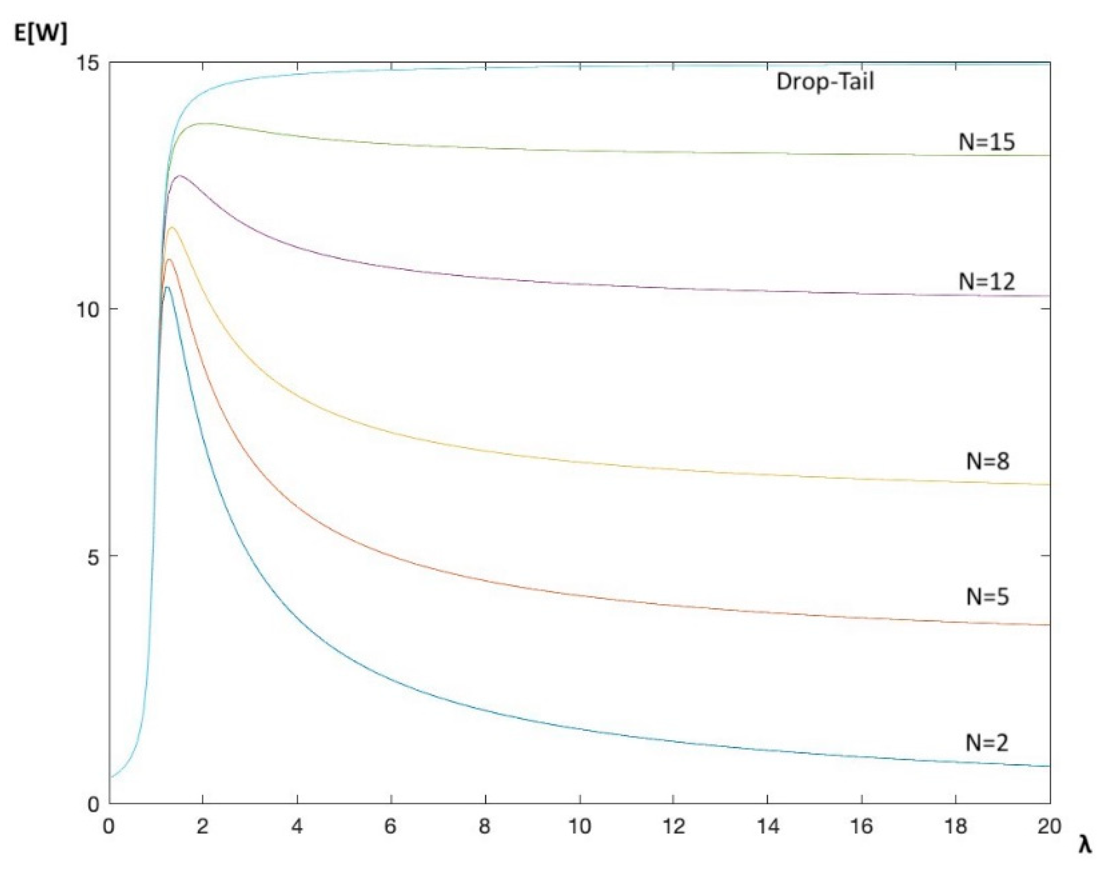
First, we considered the push-out scheme with Poisson input. The arrival rate $\lambda$ varied between 0 and 20. Figure 1 shows the average waiting time for served customers for variable push-out parameter $N$, $2\le N<16$, together with the corresponding result for the Drop-Tail strategy (i.e., when a customer arriving at a full buffer was dropped). The average waiting time increased clearly with the increasing value of $N$, with average waiting time for the Drop-Tail strategy as an upper bound. These results correspond to the results obtained in [1] for $N=2$. The difference between the two models in terms of E[W] for N = 2 is very small indeed. If the load was high, then the server only exceptionally took a vacation and hence the difference between the models was negligible in this case. In cases where the load was low, the server took vacations when, at the end of a service, the system was empty. However, unless the vacation was very long, the probability that the queue was full, and hence a push-out occurred, was extremely low. Hence, only if the vacation was long enough and the load was such that vacations occurred with non-negligible probability, and such that the queue was full at the end of a vacation, was the difference between the two models noticeable. However, even in that case, the difference was small as the models only differ in one buffer place, which was the candidate to be pushed out.

6.2. Example 2: Busty Input

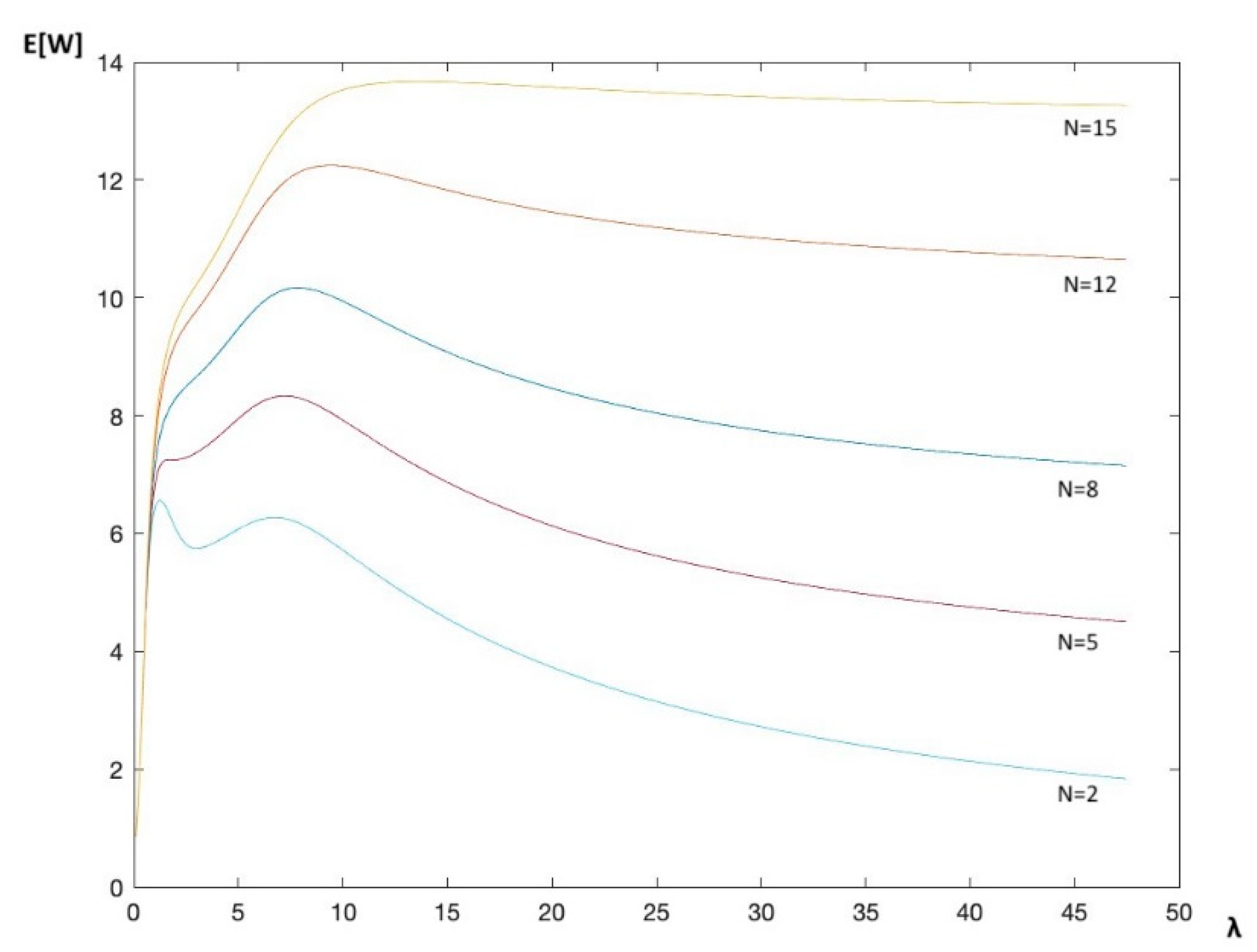
In this example, we let the input process be defined by the state transition matrix $\mathit{Q}=\left(\begin{array}{cc}0.3& 0.7\\ 0.1& 0.9\end{array}\right)$ and Poisson arrival rates $\mathit{\Lambda }=\left(k\times 6.66k\times 0.134\right),k=1,\cdots ,50$. Figure 2 shows the average waiting time for served customers for variable push-out parameter $N$, $2\le N<16$ as a function of the fundamental arrival rate $\lambda$.

From these results, we see that for a very high load, the average waiting time tends to a value close to $N-1$. Indeed, when the load is high, a tagged customer will reach position $N$ very rapidly after its arrival.

In most cases, this tagged customer will be pushed out, but if not (and this happens if between the arrival instant of the tagged customer at position $N$ and the time instant the customer in service leaves the system, no new customer arrives at the system and hence the tagged customer is not pushed-out and moves to position $N-1$), the tagged customer needs to wait $N-1$ service times before it is ready to be served. A similar observation can be made if the input is a Poisson process (Example 1).

In the above example, both states gave rise to arrival rates higher than 1 (for k > 7). If we consider an input process where some states of the arrival process lead to low arrival rates, then the above observation no longer holds.

Let

$$\mathit{Q}=\left[\begin{array}{c}0.1\hspace{1em}0.9\hspace{1em}0.0\hspace{1em}0.0\\ 0.0\hspace{1em}0.1\hspace{1em}0.9\hspace{1em}0.0\\ 0.0\hspace{1em}0.0\hspace{1em}0.2\hspace{1em}0.8\\ 0.1\hspace{1em}0.0\hspace{1em}0.0\hspace{1em}0.9\end{array}\right]$$

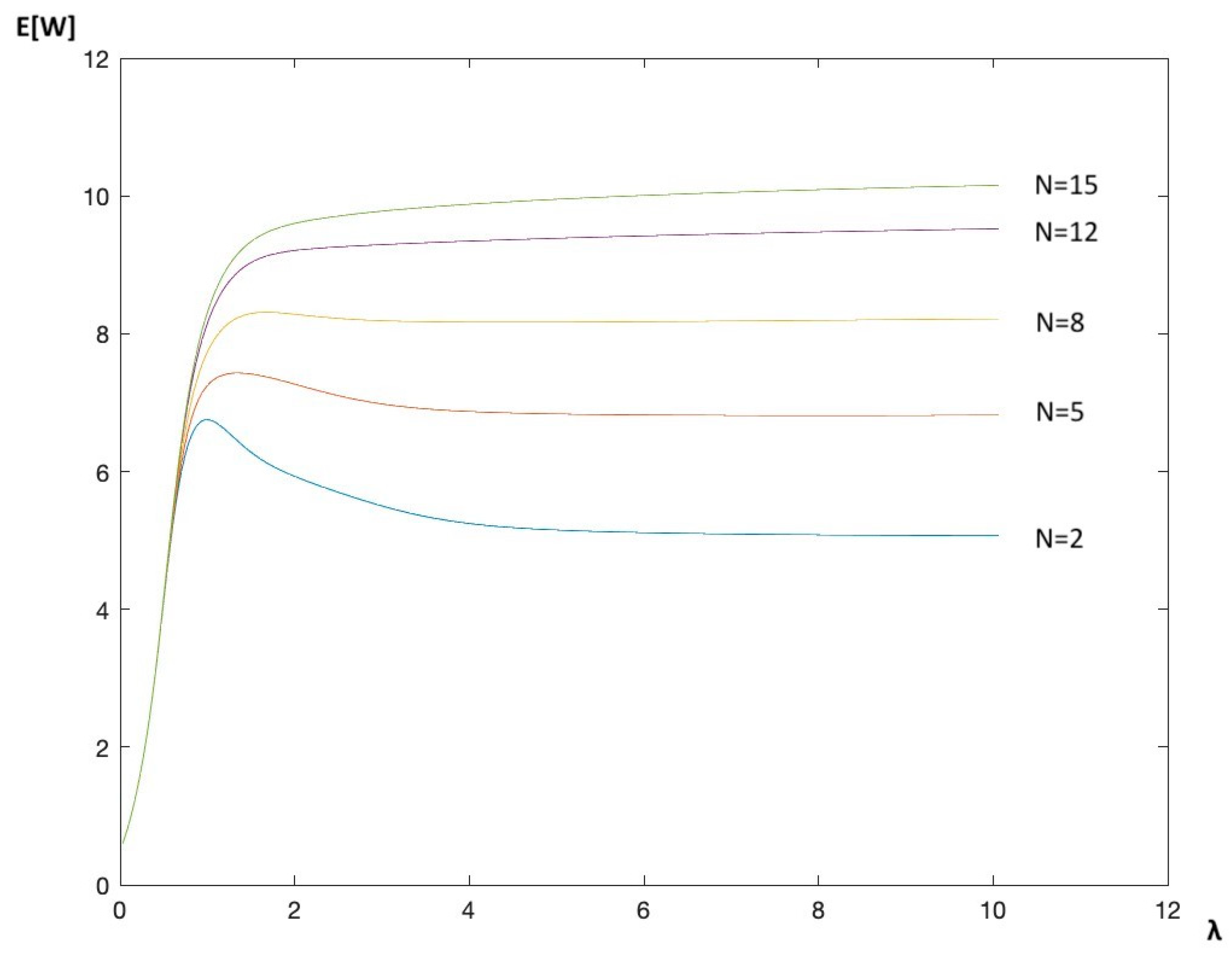
and let ${\displaystyle \Lambda }=\left(k\times 0.5,k\times 0.7,k\times 0.01,k\times 0.001\right),k=1,\cdots ,10$. Figure 3 shows the mean waiting time of a served customer for different values of $N$. The observation that the average waiting time clearly tends towards a value close to $N-1$ no longer holds. This is due to the fact that with probability $r_4=$ 0.7423 the input process is in the fourth state, and the corresponding rate is $k\times 0.001,k=1,\cdots ,10$, leading to low buffer occupancy, and hence, contrary to the previous example, a tagged customer will not reach position $N$ very rapidly after its arrival.

6.3. Example 3: Impact of the Burstiness

In this example, we investigated the impact of the burstiness of the input stream on the mean waiting time for different values of the parameter $N$. We used a simple definition for the burstiness $b$, namely the maximum arrival rate divided by the fundamental arrival rate:

$$b=\frac{\underset{i=1\cdots M}{\max }{\lambda }_i}{\mathit{r}{{\displaystyle \Lambda }}^{\prime }}$$

(40)

In this example, we let $M=3$ and kept $\mathit{Q}$ fixed, but changed the arrival rates ${\displaystyle \Lambda }=\left({\lambda }_1,{\lambda }_2,{\lambda }_3\right)$in order to have increasing values of the burstiness $b$ under constant fundamental arrival rate $\lambda$.

We let

$$\mathit{Q}=\left[\begin{array}{ccc}0.3& 0.7& 0.0\\ 0.0& 0.2& 0.8\\ 0.2& 0.0& 0.8\end{array}\right]$$

and considered three sets of arrival rates, ${{\displaystyle \Lambda }}_1=\left(8.9,12.0,0.6\right),{{\displaystyle \Lambda }}_2=\left(4.45,18.28,0.3\right),{{\displaystyle \Lambda }}_3=\left(1.112,23.0,0.075\right)$, chosen such that the fundamental arrival rate for all three sets is the same, namely $\lambda =4.0$, and the respective burstiness values are given by $b_1=3.0$, $b_2=4.57$ and $b_3=5.75$.

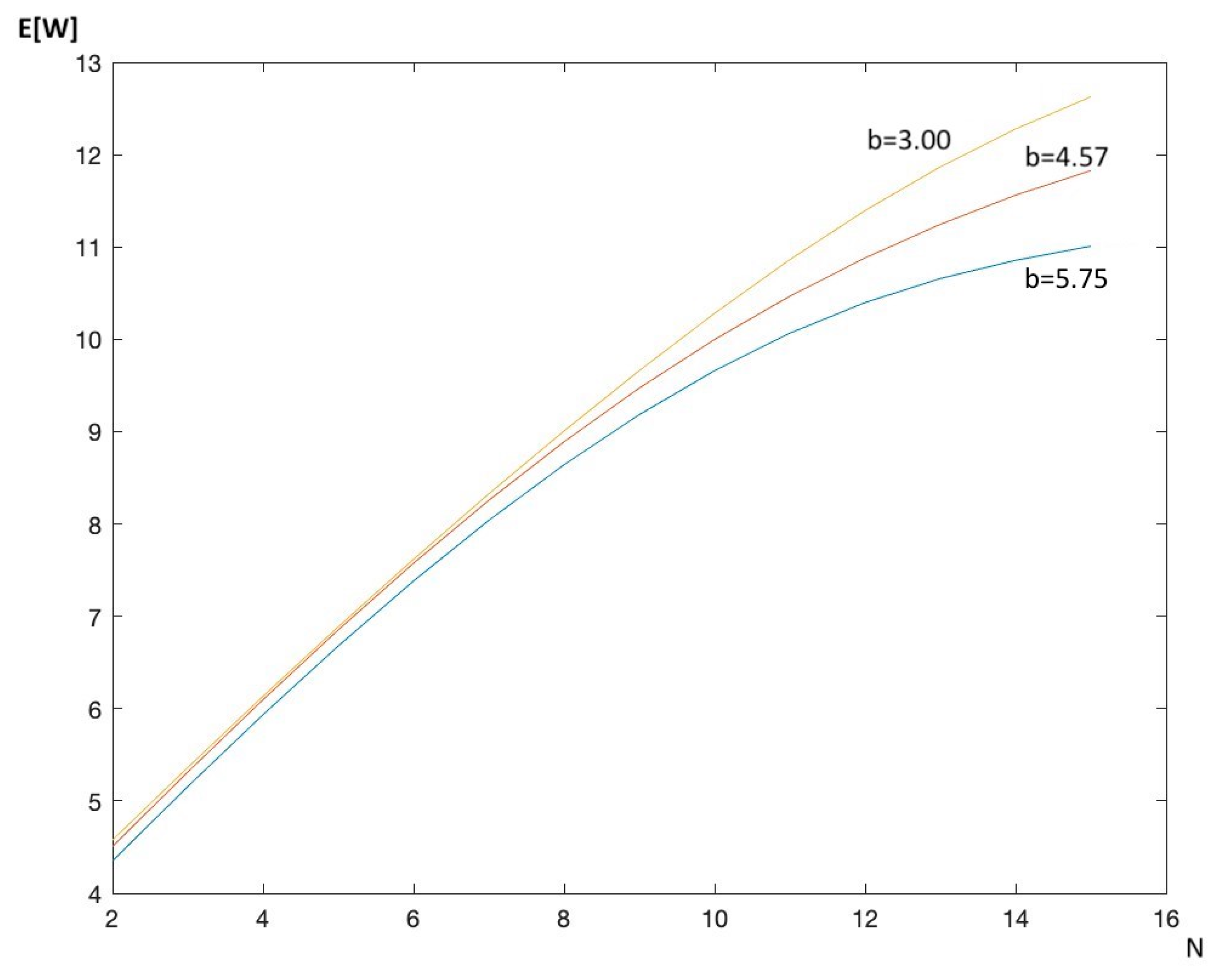
In Figure 4, we see that higher burstiness leads to shorter waiting times, in particular for larger values of the parameter $N$. Indeed, to increase the burstiness, the values of ${\lambda }_2$ were increased, but to keep the fundamental arrival rate $\lambda$ constant, the values of ${\lambda }_1$ and ${\lambda }_3$ were decreased. Since we did not change the transition matrix $\mathit{Q}$, the lower values of ${\lambda }_1$ and ${\lambda }_3$led to shorter mean waiting times.

6.4. Example 4: Waiting Time of Pushed-Out Customers

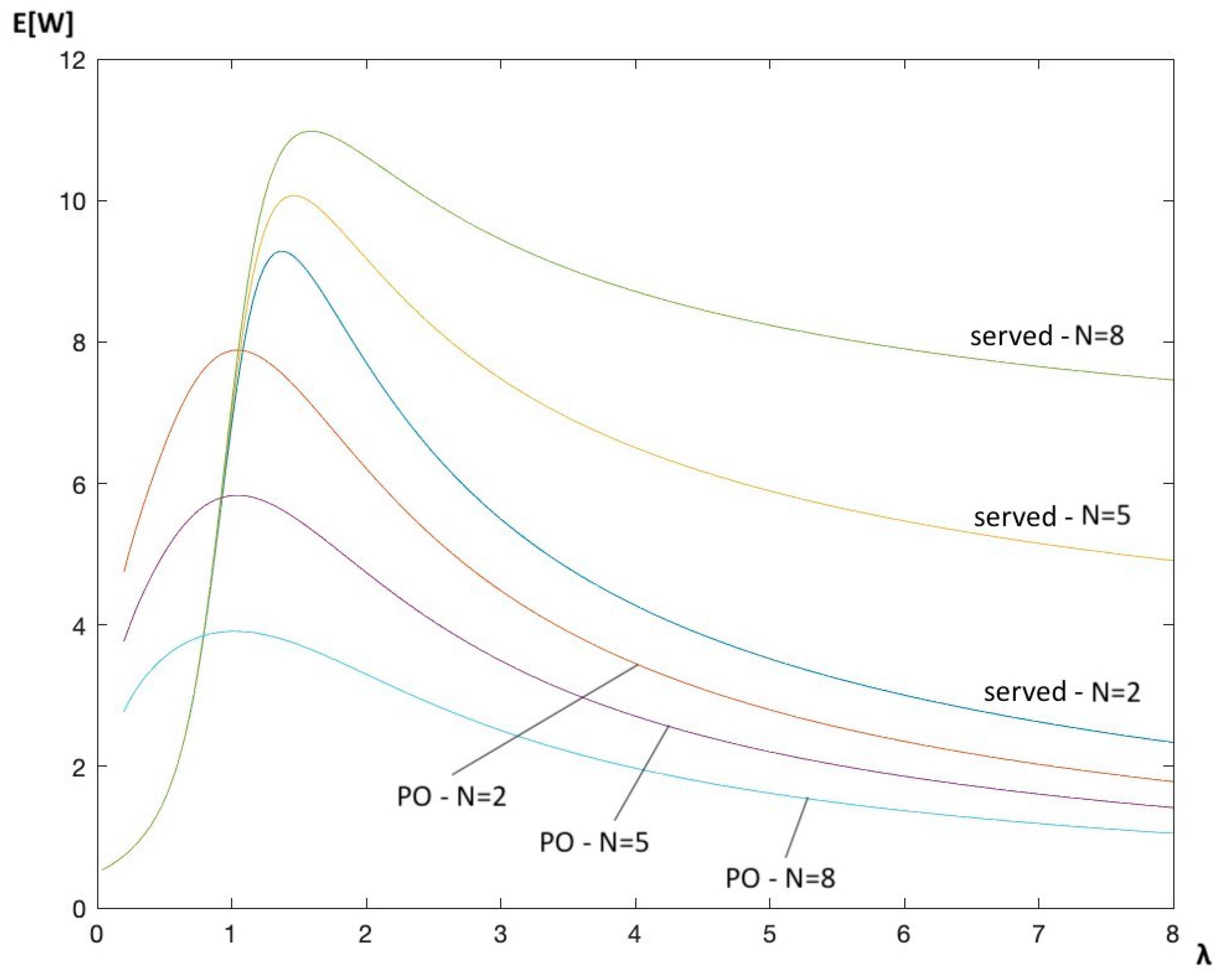
Let $\mathit{Q}=\left(\begin{array}{cc}0.3& 0.7\\ 0.1& 0.9\end{array}\right)$ and arrival rates ${\displaystyle \Lambda }=\left(k\times 0.6,k\times 0.12\right),k=1,\cdots ,50$. Figure 5 shows the average waiting time of served customers for variable push-out parameter $N$ (in Figure 5 denoted by served—$N$= 2, 5, 8) as a function of the fundamental arrival rate $\lambda$, together with the average waiting time of pushed-out customers for these values of $N$ (in Figure 5 denoted by PO—$N$ = 2, 5, 8).

Figure 5 shows that, while the average waiting time of served customers for fixed fundamental arrival rate increases with increasing values of $N$, the average time a pushed-out customer occupies a buffer space decreases for increasing $N$.

Assume that the fundamental arrival rate $\lambda$ is 2 and that the allowed average waiting time is 10, while the allowed average time a pushed-out customer stays in the queue is 5. $N$= 2 then clearly does not satisfy the latter requirement, while $N$= 5 does. This illustrates the possible trade-off between the average waiting time of a served customer and the average time a pushed-out customer is allowed to occupy a buffer place.

7. Conclusions

In this paper, we considered a queue with a finite buffer, where the server takes repeated vacations and customers arrive at the system according to a bursty arrival process. Arriving customers are admitted to the system using the following push-out strategy: when a customer arrives at a full buffer, the customer in the queue on the $N$th place ($N$ taking a value between 2 and the capacity of the queue) is pushed out and the arriving customer joins the end of the queue. This model is an immediate extension of the one considered in [1]. The LST of the waiting time distribution of a served customer is obtained. Also, the mean time a pushed-out customer occupies a buffer is derived. The numerical results coincide with the results obtained in [1] for $N=2$. For a deterministic distribution of both the vacation and service time, we see that the mean waiting time of served customers converges when the fundamental arrival rate increases, and that the mean waiting time is longer for increasing values of the parameter $N$. This means that, even for bursty arrivals, applying a push-out scheme with $N=2$ always leads to minimal average waiting time. Furthermore, higher burstiness of the input process implies a shorter mean waiting time. Finally, we show how the model can be used to determine the possible trade-off between the average waiting time of a served customer and the average time a pushed-out customer is allowed to occupy a buffer place, a relevant application when the duration of the occupancy of a buffer comes with a cost.