Exploring Dynamic Spalling Behavior in Rock–Shotcrete Combinations: A Theoretical and Numerical Investigation

Abstract

Spalling is a widespread dynamic disaster during blasting excavation in underground engineering. To clarify the coupled dynamic response and spalling behavior of an underground tunnel with a spray anchor, an investigation based on the rock–shotcrete combination was conducted using theoretical and numerical methods. The mathematical representation of stress wave propagation between rock and shotcrete was deduced based on the elastic stress wave theory. A novel method for predicting the location and time of initial spalling in a rock–shotcrete combination was proposed. A numerical simulation was conducted to verify the validity of the proposed theoretical method. In addition, the effect of the material’s tensile strength, the loading amplitude, and the thickness of shotcrete on the stress evolution and spalling characteristics was studied. The results demonstrate that the initial spalling locations are sensitive to the relationship between the normalized tensile strength of the rock, shotcrete, and interface. A high incident amplitude can cause the initial spalling in rock, and the shotcrete or rock–shotcrete interface can cause initial spalling due to a low incident amplitude. The stress evolution and spalling characteristics are sensitive to the thickness of shotcrete. The location of the initial spalling failure changes with the thickness of the shotcrete. An appropriate increment in thickness and normalized strength of the shotcrete is beneficial to the dynamic stability of underground engineering.

1. Introduction

In underground engineering, dynamic disturbances caused by blasting and earthquakes can cause some unexpected dynamic disasters, such as spalling [1,2], zoning disintegration [3], and rockburst [4,5]. Therefore, it has gradually become important to maintain the dynamic stability of underground engineering. When spalling occurs, the surrounding rock and support usually break apart layer by layer in a sheet-like manner, causing deterioration of the surrounding rock and the support, which poses serious challenges to the support design and stability evaluation of underground buildings. Therefore, a thorough understanding of the spalling mechanism and its influence on engineering structures is extremely significant.

The phenomenon of rock spalling has been a topic of considerable research interest thus far. In underground excavation or mining, blasting usually causes the spalling of adjacent tunnels, caverns, and pillars. For example, at the −600 m level of Kaiyang Phosphate Mine, the blasting excavation of a new tunnel has induced spalling in the surrounding rock of the adjacent tunnel (seen in Figure 1a) [6]. In the Chambishi copper mine, Zambia, spalling in shotcrete in the tunnels was also induced during a blasting operation in a stope (seen in Figure 1b). In addition, in the Heiniudong copper mine, China, the rock–shotcrete interface in the tunnel has also experienced this spalling phenomenon due to frequent blasting operations nearby (seen in Figure 1c). Generally, spalling is regarded as dynamic tensile fracturing, which is related to the reflection of stress waves on the building surfaces or structural planes [6,7]. Therefore, some scholars have analyzed the phenomenon of rock spalling based on the propagation characteristics of stress waves [8,9,10]. For example, Weerheijm and Doormaal [8] believe that spalling is a tensile failure caused by pressure waves in an area far from the free surface, and the failure phenomenon is related closely to the wave impedance of the material, impulse load, loading rate, and notch morphology. Li et al. [9] analyzed the spalling problem in a single medium and found that the spalling usually occurs at the location where the net tensile stress reaches the dynamic tensile strength of the rock mass after the superimposition of a stress wave. Zhao et al. [6] analyzed the spalling problem of existing tunnels caused by adjacent tunnel excavation through theoretical and numerical simulation. The results show that spalling damage of existing tunnels is mainly related to the radial stress concentration caused by short incident waves, and the circumferential and radial stress around the tunnel is negatively correlated with the number of cracks. Certainly, in underground environments, spalling is often induced by the coupling of dynamic loads and static loads [11,12,13,14,15]. For example, Qiu et al. [11] found that with the increase in mining depth, the spalling around a tunnel caused by blasting loads would intensify, while the damage in other areas would be suppressed. Moreover, Li et al. [15] also indicated that the lateral pressure coefficient, excavating depth, blasting wavelength, etc., will affect the formation of spalling cracks, rockbursts, and other damages around a tunnel.

Generally speaking, the dynamic tensile strength of rock masses can be obtained through direct or indirect tension methods [16,17]. As a typical tensile fracturing test, the spalling test can usually be used to determine the dynamic tensile strength of rock mass materials, also known as the “spalling strength”, based on SHPB devices [18,19]. Compared with the dynamic Brazilian splitting test or dynamic direct tensile test, the spalling test usually combines high accuracy and convenience. To this end, several scholars have conducted sufficient research on the spalling test [8,20,21,22]. For example, Kubota et al. [20] conducted spalling tests of sandstone using emulsion explosives and filled water and proposed a method for confirming rock spalling strength based on the velocity at the free end of the sample. Zhao et al. [21] conducted a study on the spalling strength and failure characteristics of sandstone and proposed a modified stress wave analysis method to calculate the dynamic tensile strength of rock-like materials. At the same time, they also indicated that the spalling failure and spalling strength will be affected by the confining pressure. Cho et al. [22] compared the dynamic and static tensile strength characteristics of Inada granite and Tag tuff, and the results showed that the inhomogeneity of rock would affect the strain-rate dependence of the tensile strength.

Additionally, as an important component of underground structures, the dynamic properties of support materials, especially their dynamic tensile properties, have also attracted the attention of some scholars [23,24,25]. For example, Erzar and Forquin [25] also carried out laboratory spalling tests and numerical simulations on concrete and determined the dynamic tensile strength based on three methods. The results showed that the spalling strength of concrete samples had a strong strain-rate dependence. Werheijm and Doormaal [8] also observed that the spalling behavior of concrete exhibits strong strain-rate dependence. Zhang et al. [26] found that the spalling strength of concrete is strengthened by the addition of steel fiber, and the strengthening degree is linearly related to the fiber slenderness ratio.

Whether it was conducted in the field or in laboratory experiments, the past research focused more on one single medium. As shotcrete has gradually become an important support means to maintain the stability of underground structures, the spalling behavior around the structures with shotcrete has shifted from the response problem of one medium to the coupled response problem of a rock–shotcrete combination or multiple media (as shown in Figure 2), which has been a subject of considerable interest. For example, Ahmed and Ansell [27] conducted a laboratory experiment on a concrete bar with cement-based mortar applied to it and partly verified the previously recommended maximum allowed peak particle vibration velocities in their numerical simulation investigation [28]. Luo et al. [29] investigated the dynamic tensile behavior of rock–shotcrete interface geometry exposed to vibrations and found that the bearing capacity of rock–shotcrete interfaces varies with the height of the micro sawtooth. Shen et al. [30] investigated the influence of the hydrophilicity and roughness of the rock interface on interfacial bond strength. Zhou et al. [31] conducted quasi-static and dynamic splitting tests to investigate the effect of interface inclination on the mechanical properties, dissipated energy, and failure characteristics of rock–concrete bi-material discs. Qiu et al. [32] investigated the effects of the elastic modulus and tensile strength of shotcrete on the dynamic tensile behavior of rock–shotcrete interfaces. The results showed that increasing shotcrete elastic modulus to a certain extent can achieve better tensile performance than increasing tensile strength. Zhu et al. [10] conducted a numerical simulation to study the dynamic response of rock joints and underground openings with shotcrete subject to tensile stress wave and found that shotcreting with sufficient thickness could effectively reinforce the surrounding rock and reduce the area of disturbed zones facing dynamic extension.

However, these studies on the rock–shotcrete interface focus more on the overall mechanical response of the combination. The understanding of stress wave propagation in a rock–shotcrete combination under dynamic extension is still in its infancy. The interaction and its internal mechanism remain vague. In addition, few studies have predicted the time and location of spalling failures occurring in underground openings with shotcrete lining. Thus, more attention should be focused on this subject. Furthermore, owing to the uncertainty of shotcrete construction, including the uneven thickness and strength of shotcrete, the location and intensity of spalling are evidently variable. Considering the randomness of dynamic disturbance, the occurrence of spalling is also more complicated. Therefore, accurate prediction of the location, time, and intensity of spalling is extremely challenging. Thus, in this paper, the dynamic spalling problem of a rock–shotcrete combination was studied through theoretical and numerical simulation methods. The stress evolution and spalling characteristics, such as initial spalling location and time, were analyzed during the stress wave propagation along a rock–shotcrete combination and a theoretical method was proposed to predict the spalling behavior of a rock–shotcrete combination. In addition, the influences of the material’s tensile strength, the loading conditions, and the thickness of shotcrete were further studied.

2. Mathematical Representation of Stress Wave Propagation in Rock–Shotcrete Interface Bar

2.1. Propagation Process of Stress Wave in Rock–Shotcrete Combination

As illustrated in Figure 3, we assume that a half-sine wave with a period T and length λ propagates from one end of the rock to the end of the shotcrete. The propagation process of a stress wave can be presented as discussed in this section. According to Li [33] and Wang [34], this ideal stress wave can usually be replaced by a half-sine wave, triangular wave, or rectangular wave in theoretical analysis. It has been confirmed that this complex blast wave can be replaced by simplified half-sine or triangular waves, causing the main waveform of the blast wave to be similar to these [4,11,35]. In this study, a half-sine wave was used to analyze the propagation process of stress waves in a rock–shotcrete combination, and it can be expressed in Equation (1) according to Li [33]. Note that the interface between rock and shotcrete is defined as a joint in this study. As shown in Figure 3, the compression stress wave first travels along the rock bar until reaching the joint, i.e., the interface between the rock and shotcrete. The arrows in Figure 3 refer to direction of the wave propagation. Afterward, the first reflection and transmission occur (named i) because of the difference in the acoustic impedances of the two materials. Thereafter, the transmitted stress wave in the shotcrete arrives at the free surface, and a perfect reflection occurs at this moment (named ii). After the process (ii), the reflected wave of the shotcrete reaches the joint again, and the second reflection and transmission at the joint can occur (named iii). Similar to processes i–ii, the new reflected wave propagates to the free surface, causing a perfect reflection again (iv). Furthermore, similar processes (v, vi, …) continue until the stress in the shotcrete is dissipated.

$$\sigma \left(t\right)={\sigma }_m\sin \left(\frac{\pi }{T}t\right)$$

(1)

where σ₀ denotes the amplitude of the stress wave. T represents the period of the stress wave.

2.2. Overview of Reflection and Transmission Coefficients

Without considering multiple reflections between the materials, if an elastic stress wave propagates from one material to another along the normal direction of the interface between them, based on the stress wave theory [34], the ratio of acoustic impedance of the two materials can be obtained:

$$\omega =\frac{{\rho }_1{C}_1}{{\rho }_2{C}_2}$$

(2)

where $\omega$ is the ratio of the acoustic impedance of the two materials. ρ₁, ρ₂, C₁, and C₂ are the density and wave velocity.

As shown in Figure 3, two cases are included during the reflection and transmission at the rock–shotcrete interface. In the first case, the stress wave is transmitted from the rock into the shotcrete, and in the second case, the stress wave is transmitted from the shotcrete into the rock. Thus, the reflection and transmission coefficients in the two cases might differ. Based on the stress wave propagation theory [34], for the first case, the transmission coefficient T₁ and reflection coefficient F₁ can be expressed using Equations (3) and (4). Based on the analysis of Section 2.1, it is only process i that meets the requirements of this case.

$$T_1=\frac{2}{1+\omega }=\xi$$

(3)

$$F_1=\frac{1-\omega }{1+\omega }=\xi -1$$

(4)

For the second case, i.e., processes iii, v, vii, …, the ratio of acoustic impedance n in Equations (5) and (6) was replaced by $1/\omega$; thereby, the transmission coefficient T₂ and reflection coefficient F₂ can be obtained.

$$T_2=\frac{2}{1+\raisebox{1ex}{$1$}\!\left/ \!\raisebox{-1ex}{$\omega $}\right.}=2-\xi$$

(5)

$$F_2=\frac{1-\raisebox{1ex}{$1$}\!\left/ \!\raisebox{-1ex}{$\omega $}\right.}{1+\raisebox{1ex}{$1$}\!\left/ \!\raisebox{-1ex}{$\omega $}\right.}=1-\xi$$

(6)

In addition, based on the stress wave propagation theory [32], when the perfect reflection occurred on the free surface, i.e., processes ii, iv, vi, …, the transmission coefficient T₃ and reflection coefficient F₃ could be expressed.

$$T_3=0$$

(7)

$$F_3=-1$$

(8)

Based on the stress wave theory [33,34], if the acoustic impedance of rock is greater than that of shotcrete, the reflected stress wave, which is in the rock, will be the tensile stress in process I (seen in Equations (2) and (4)). Additionally, the transmitted stress wave, which is in the shotcrete, will be compressive stress, and its amplitudes will be smaller than the incident stress wave (seen in Equations (2) and (3)). In processes ii, iv, vi, …, due to the wave impedance of the air behind the free surface being 0, the new reflected stress wave maintains the same amplitude according to Equation (8), and the stress type is converted from compression to tensile stress, or vice versa. However, for processes iii, v, vii, …, the reflection coefficient is greater than 0 but less than 1 according to Equation (6); thus, the new reflective stress in the shotcrete maintains the original stress type. However, its amplitude decreases accordingly. Furthermore, the rock is disturbed again by the new transmitted stress. Additionally, because the actual rock mass was a semi-infinite body, the rock bars in this study were assumed to be sufficiently long, and the reflection at the input end of the rock was not considered.

2.3. Stress Wave Representation in Rock–Shotcrete Combination

The two points A and B located within the shotcrete and rock, respectively, were first determined to understand the evolution of stress waves in rock and shotcrete in a better way, as shown in Figure 4. The distances between the two points and the free surface were expressed as L_A and L_B, respectively, and the length of the shotcrete was expressed as δ. The time when the incident wavefront reached the joint between the rock and shotcrete was assumed as the initial moment, and the x-coordinate of this free surface was defined as 0. The half-sine wave, which was loaded into the rock, could be tracked by Equation (1).

Based on the stress wave theory [34], a total stress wave can be synthesized by the superposition of wavelets generated at each time. Thus, the stress waves in rock and shotcrete can be regarded as the sum of the new stress after each reflection, transmission, and original stress. Because the period, wavelength, and amplitude of the initial incident stress wave might vary, the time t, distances L_A and L_B, length δ, and stress ${\sigma }_0$ were normalized. The normalization process was primarily based on the period T, wavelength λ_B, and amplitude σ_m of the initial incident wave, as shown in Equations (9)–(14). Here, the symbol $\tau$ represents the normalized time. The symbols $x_A$, $x_B$, and $x_d$ represent the normalized locations of point A, point B, and the joint, respectively. The symbol $\sigma$ represents the normalized stress. Additionally, a new parameter η was introduced to represent the relationship between the wavelength in the shotcrete ${\lambda }_A$ and that in the rock ${\lambda }_B$, as shown in Equation (14). The detailed propagation process of stress waves in a rock–shotcrete combination is provided in Appendix A.

$$\tau =\frac{t}{T}$$

(9)

$$x_A=\frac{L_A}{{\lambda }_B}$$

(10)

$$x_B=\frac{L_B}{{\lambda }_B}$$

(11)

$$x_d=\frac{\delta }{{\lambda }_B}$$

(12)

$$\sigma =\frac{{\sigma }_0}{{\sigma }_m}$$

(13)

$$\eta =\frac{{\lambda }_A}{{\lambda }_B}=\frac{C_A\times T}{C_B\times T}=\frac{C_A}{C_B}$$

(14)

As summarized in Appendix A, the stress wave at point A in any stage can be derived as follows:

$${\sigma }_N^A=\left\{\begin{array}{ll}{(-1)}^{K_1}{\xi (1-\xi )}^{K_2}\sin \pi (\tau -{\tau }_N^A)& {\tau }_N^A\le \tau \le {\tau }_N^A+1\\ 0& \tau <{\tau }_N^A\mathrm{or}\tau >{\tau }_N^A+1\end{array}\right.$$

(15)

$${\tau }_N^A=\left\{\begin{array}{ll}\frac{K_3\delta -L_A}{\eta \times {\lambda }_B}=\frac{K_3\times x_d-x_A}{\eta }& N=1,3,5,7\dots \\ \frac{K_3\delta +L_A}{\eta \times {\lambda }_B}=\frac{K_3\times x_d+x_A}{\eta }& N=2,4,6,8\dots \end{array}\right.$$

(16)

$$\left\{\begin{array}{lll}{K}_1=K_2=\frac{N-1}{2}& K_3=N& N=1,3,5,7\dots \\ K_1=\frac{N}{2}\hspace{1em}{K}_2=\frac{N-2}{2}& K_3=N-1& N=2,4,6,8\dots \end{array}\right.$$

(17)

Stress expressions at point B in any stage are given by

$${\sigma }_0^B=\left\{\begin{array}{ll}\sin \pi (\tau +{\tau }_0^B)& -{\tau }_0^B\le \tau \le 1-{\tau }_0^B\\ 0& \tau <{\tau }_0^B\mathrm{or}\tau >{\tau }_0^B+1\end{array}\right.\begin{array}{cc}& N=0\end{array}$$

(18)

$${\sigma }_1^B=\left\{\begin{array}{ll}(\xi -1)\sin \pi (\tau -{\tau }_1^B)& {\tau }_1^B\le \tau \le {\tau }_1^B+1\\ 0& \tau <{\tau }_1^B\mathrm{or}\tau >{\tau }_1^B+1\end{array}\right.\begin{array}{cc}& N=1\end{array}$$

(19)

$${\sigma }_N^B=\left\{\begin{array}{ll}{(-1)}^{K_1}\xi {(1-\xi )}^{K_2}(2-\xi )\sin \pi (\tau -{\tau }_N^B)& {\tau }_N^B\le \tau \le {\tau }_N^B+1\\ 0& \tau <{\tau }_N^B\mathrm{or}\tau >{\tau }_N^B+1\end{array}\right.\begin{array}{c}N=3,5,7,9\dots \end{array}$$

(20)

$${\tau }_N^B=\left\{\begin{array}{ll}{\mathrm{x}}_{\mathrm{B}}-{\mathrm{x}}_{\mathrm{d}}& N=0,1\\ \frac{K_3\delta }{{\lambda }_A}+\frac{L_B-\delta }{{\lambda }_B}=\left(\frac{K_3}{\eta }-1\right)\times x_d+x_B& N=3,5,7,9\dots \end{array}\right.$$

(21)

$$K_1=\frac{N-1}{2}\hspace{1em}{K}_2=\frac{N-3}{2}\hspace{1em}{K}_3=N-1\hspace{1em}N=3,5,7,9\dots$$

(22)

The total stress wave at points A and B can be obtained by superimposing the stress components at each stage, as expressed in Equations (23) and (24).

$${\sigma }^A={\sigma }_1^A+{\sigma }_2^A+{\sigma }_3^A+{\sigma }_4^A+{\sigma }_5^A+{\sigma }_6^A+{\sigma }_7^A+\dots$$

(23)

$${\sigma }^B={\sigma }_0^B+{\sigma }_1^B+{\sigma }_3^B+{\sigma }_5^B+{\sigma }_7^B+\dots$$

(24)

2.4. Modifications of Stress Wave Due to the Nonlinear Elastic Behavior of Joints

Formulas (15) and (18)–(20) are primarily based on the assumption of the linear elastic behavior of joints. However, the joint deformation behavior in the natural rock mass or some numerical models was often nonlinear elastic, and the displacement and deformation on both sides of the joint were discontinuous [36,37]. Therefore, when waves with different frequencies arrive at joints, cracks, and other geological defects, the wave velocity through the geological defects may be different, which is usually called the wave dispersion effect [38,39]. In numerical simulation or practical engineering, this incident wave is usually composed of multiple frequency wavelets, rather than an ideal wave with a unique frequency (such as the half-sine wave shown in Equation (1)). Therefore, when the incident wave passes through the joint, the wave velocity of each phase point in the wave may change, and as a result, the period of the reflected wave and the transmitted wave may be different from that of the incident wave. Furthermore, the transmitted and reflected coefficients might be different from those of linear elastic joints, as shown in Figure 5. For the convenience of subsequent analysis, a few parameters were determined. When the stress wave propagates from the medium A to B, the transmission attenuation coefficient f₁ is defined as the ratio of the transmission coefficient of the nonlinear elastic joint to that of the linear elastic joint, and the reflected attenuation coefficient f₂ is defined as the ratio of the reflected coefficients between the two types of joints. In contrast, the period extension coefficient $p_1$ is defined as the ratio of the transmission period of the nonlinear elastic joint to that of the linear elastic joint. Similarly, when the stress wave propagates from medium B to A, its transmission attenuation coefficient f₃, the reflected attenuation coefficient f₄, and the period extension coefficient $p_2$ can be obtained.

Considering the nonlinear elastic characteristics of the joints, Equations (15), (19) and (20) can be represented as

$${\sigma }_N^A=\left\{\begin{array}{ll}{(-1)}^{K_1}{f_1{f}_4}^{K_2}{\xi (1-\xi )}^{K_2}\sin \frac{\pi }{{p_1{p}_2}^{K_2}}(\tau -{\tau }_N^A)& {\tau }_N^A\le \tau \le {\tau }_N^A+{p_1{p}_2}^{K_2}\\ 0& \tau <{\tau }_N^A\mathrm{or}\tau >{\tau }_N^A+{p_1{p}_2}^{K_2}\end{array}\right.$$

(25)

$${\sigma }_1^{\mathrm{B}}=\left\{\begin{array}{ll}{f}_2(\xi -1)\sin \frac{\pi }{p_1}(\tau -{\tau }_1^{\mathrm{B}})& {\tau }_1^B\le \tau \le {\tau }_1^B+p_1\\ 0& \tau <{\tau }_1^B\mathrm{or}\tau >{\tau }_1^B+p_1\end{array}\right.\begin{array}{cc}& N=1\end{array}$$

(26)

$${\sigma }_N^B=\left\{\begin{array}{ll}{(-1)}^{K_1}{f}_1{f_3{f}_4}^{K_2}\xi {(1-\xi )}^{K_2}(2-\xi )\sin \frac{\pi }{{p_1{p}_2}^{K_1}}(\tau -{\tau }_N^B)& {\tau }_N^B\le \tau \le {\tau }_N^B+{p_1{p}_2}^{K_1}\\ 0& \tau <{\tau }_N^B\mathrm{or}\tau >{\tau }_N^B+{p_1{p}_2}^{K_1}\end{array}\right.$$

(27)

By substituting Equations (16), (17), (21) and (22) into Equations (18), (25), (26) and (27), respectively, we can obtain the stress wave at points A and B at each stage. Afterward, by substituting Equations (18) and (25)–(27) into Equations (23) and (24), the total stress at two points can be obtained again. Furthermore, when the parameters f₁, f₂, f₃, f₄, P₁, and P₂ are equal to 1, Equations (25)–(27) can characterize the stress wave characteristics of linear elastic joints. In addition, by transforming the locations and times of points A and B, the stress history of any point in the rock–shotcrete combination can be obtained.

3. Theoretical Prediction for Initial Spalling of Rock–Shotcrete Combination

In general, for a homogeneous material, the position with the largest stress is often the most prone to failure. Therefore, the initial spalling, which is primarily caused by the tensile stress, may be at the location where the stress wave first reaches the tensile strength. In this study, because the rock–shotcrete combination involved three parts, namely the rock, the shotcrete, and the joint between the rock and shotcrete, the initial spalling depended on the difference between the stress states of the three parts and their respective tensile strengths. Based on Section 2, the stress of the rock–shotcrete combination at any location at any moment could be obtained from Formulas (23) and (24). Therefore, the maximum tensile stress and its corresponding location in the rock–shotcrete combination at each moment could be recorded. For this purpose, MATLAB R2013b code was used. Because the compression stress did not induce spalling failure, this study primarily focused on the effect of tensile stress. Therefore, the compression stress defaulted to 0 in the MATLAB code for the convenience of analysis. As shown in

Table 1. List of studies on rock–shotcrete interface.

Year	Researchers	Works
2012	Ahmed and Ansell [27]	conducted a laboratory experiment and verified the previous recommendations
2012	Ahmed [28]	conducted numerical simulation and recommended maximum allowed peak particle vibration velocities
2017	Luo et al. [29]	investigated the effect of rock–shotcrete interface geometry on the dynamic tensile behavior
2019	Shen et al. [30]	investigated the influence of the hydrophilicity and roughness of the rock interface on interfacial bond strength
2020	Zhou et al. [31]	conducted splitting tests to investigate the effect of interface inclination on the mechanical properties of rock–concrete bi-material discs
2020	Qiu et al. [32]	investigated the effects of elastic modulus and tensile strength of shotcrete on the dynamic tensile behavior of rock–shotcrete interfaces
2021	Zhu et al. [10]	conducted numerical simulation to study dynamic response of underground openings with shotcrete

, the stress wave at points A and B depends not only on their locations (x_A, x_B) and time (τ) but also on the thickness of the shotcrete (x_d). Considering the thickness of shotcrete δ = 0.5 ηλ_B as an example, a method for predicting initial spalling is introduced in detail. The maximum tensile stress and its corresponding location are presented in Figure 6. The mechanical parameters of rock and shotcrete were firstly input, and they are referenced by the numerical results in Section 4.1. The densities of rock and shotcrete were 2628 and 1866 kg·m⁻³, respectively. The wave velocities of rock and shotcrete were 3700 and 2510 m/s, respectively. The parameters f₁, f₂, f₃, and f₄ were 0.96, 0.72, 0.98, and 0.94, respectively. The parameters P₁ and P₂ were 1.23 and 1.14, respectively.

As shown in Figure 6a–c, the blue lines represent variations in the maximum tensile stress σ_tmax in rock and shotcrete at the joint, respectively. The orange lines represent their corresponding locations. Once the tensile strength σ_t-rock of rock was determined, the failure moment τ_f-rock could be determined using the blue curve. In addition, its failure location x_f-rock could be determined based on the corresponding orange line, as shown in Figure 6a. In a similar way, the failure moments and locations of the shotcrete and joint could be obtained, as marked in Figure 6b,c. Based on the three failure moments (τ_f-rock, τ_f-shot, and τ_f-joint), one part failed first if its failure moment was ahead of the others. The minimum failure moment could be determined as the time of initial spalling of the rock–shotcrete combination (as shown in Formula (32)), and its corresponding location could be regarded as the location of the initial spalling. When the initial spalling occurs, the stress state in the three materials might change because of new cracks. Therefore, the above method might not be suitable for subsequent failure analyses.

$${\tau }_f=\min ({\tau }_{f\text{-}rock},{\tau }_{f\text{-}shot},{\tau }_{f\text{-}joint})$$

(28)

The aforementioned accurate material parameters, such as tensile strength and wave velocity, are very crucial for determining the location and time of initial spalling. However, the material parameters of natural rock mass, such as strength, elastic modulus, and wave velocity, usually exhibit a few uncertain characteristics [40,41]. Therefore, the analysis is limited to an accurate determination of the location and time of the initial spalling in the in situ condition based on the deterministic material parameters obtained from laboratory tests. Additionally, in the in situ condition, the failure time and location of the spalling often fluctuated within a certain range. Therefore, in the in situ condition, the potential time and location ranges of the initial spalling should have been determined according to the upper and lower limits of the material parameters.

In contrast, even if the strength of the material was unknown, the maximum time and maximum location ranges of the initial spallation could be inferred. Considering Figure 6 as an example, the initial spalling might occur in two stages in the rock, such as when τ = 0.5–1.088 and τ > 1.725. In the first stage (τ = 0.5–1.088 T), the location curve showed a V-shaped change, and the corresponding location was in the range x = 0.532–0.811. In the second stage (τ > 1.725), the maximum tensile stress remained constant, and the corresponding location increased with time. However, for τ = 1.088–1.725, its corresponding location x was always 0.339, which was exactly located at the joint (x_joint). Therefore, the initial spalling occurred at the joint instead of the rock at this stage. Similarly, the time of initial spalling in the shotcrete was τ = 1.227–1.567, and the corresponding location was in the range x = 0.242–0.338. For the joint, the time for initial spalling to occur was τ = 0.951–2.345. Therefore, the maximum time and maximum location ranges of the initial spalling in the three materials are summarized in Equations (29)–(32). In addition, since the spalling location x, spalling time τ, and tensile strength σ_t were normalized, the actual failure location, time, and stress were calculated by multiplying their respective wavelength ${\lambda }_B$, period T, and stress amplitude ${\sigma }_m$.

$$\left\{\begin{array}{l}{\tau }_{f\text{-}rock}=0.5~1.088\\ x_{f\text{-}rock}=0.532~0.811\end{array}\right.$$

(29)

$$\left\{\begin{array}{l}{\tau }_{f\text{-}rock}>1.725\\ x_{f\text{-}rock}>0.339\end{array}\right.$$

(30)

$$\left\{\begin{array}{l}{\tau }_{f\text{-}shot}=1.227~1.567\\ x_{f\text{-}shot}=0.242~0.338\end{array}\right.$$

(31)

$$\left\{\begin{array}{l}{\tau }_{f\text{-}joint}=0.951~2.345\\ x_{f\text{-}joint}=0.339\end{array}\right.$$

(32)

4. Comparison between Numerical Investigation and Theoretical Investigation

4.1. Numerical Modeling

To verify the aforementioned theoretical method for predicting initial spalling, two PFC2D models consisting of rock, shotcrete, and joint were used to perform the numerical simulation investigation, as shown in Figure 7, in which red arrows refers to the incident stress wave. Additionally, model A was used in subsequent analyses to compare the theoretical and numerical results, and model B was applied to conduct pretests for determining the stress wave propagation properties of joints. In addition, the parallel bond model (PBM) was applied to synthesize the rock and shotcrete, and the smooth joint model (SJM) was applied to represent the joint. The particle radius was 0.25–0.5 mm. For model A, the width of the rock–shotcrete combination was set to 0.035 m, the length of rock was set to 1.39 m, and the length of shotcrete was set to $0.5\eta {\lambda }_B$, namely $\delta =0.22\mathrm{m}$. For model B, the width was the same as model A, and the lengths of rock and shotcrete were 0.81 and 0.8 m, respectively. As described in Section 2 and Section 3, the stress history of any point of the rock–shotcrete bar, possible spalling location, and spalling time can be obtained. In addition, different normalized tensile strengths might cause a change in the location and time of the initial spalling. Thus, two groups of materials with different joint strengths were considered. In order to determine the mechanical properties of rock and shotcrete, uniaxial compression tests in the laboratory were carried out. And a series of numerical trial and error programs based on uniaxial compression tests were executed to match the experimental data. Furthermore, a spalling testing program was executed to obtain the tensile strength of rocks and shotcrete. The components of these two groups of materials and their macroscopic mechanical parameters are shown in

Table 2. Macroscopic mechanical parameters of materials.

Group	Component	Density ρ, kg·m−3	Tensile Strength σt, MPa	UCS, MPa	Young’s Modulus E, GPa	Poisson Ratio υ	P-Wave Velocity λ
Group 1	Rock	2628	14.13	146.6	31.6	0.15	3700
	Shotcrete	1866	11.84	57.4	10.5	0.23	2510
	Joint 1	-	6.95		-	-	-
Group 2	Rock	2628	14.13	146.6	31.6	0.15	3700
	Shotcrete	1866	11.84	57.4	10.5	0.23	2510
	Joint 2	-	9.80		-	-	-

. Accordingly, the microscopic mechanical parameters of these components are listed in

Table 3. Microscopic mechanical properties of materials.

Parameters	Analog Component
	Rock	Shotcrete	Joint 1	Joint 2
Particle density (kg/m3)	2628	1866	-	-
Particle radius (mm)	0.25–0.5	0.25–0.5	-	-
Damping	0.0	0.0	-	-
Friction angle $\varphi$	45°	45°	-	-
Linear contact modulus Ec (GPa)	19	7	-	-
Linear contact stiffness ratio (kn/ks)	1.08	1.65	-	-
Parallel bond modulus ${\overline{E}}_c$ (GPa)	19	7	-	-
Parallel bond stiffness ratio (${\overline{k}}_n/{\overline{k}}_s$)	1.08	1.65	-	-
Joint normal stiffness (${{\overline{k}}_n}^{\prime }$)	-	-	1 × 1014	1 × 1014
Joint shear stiffness (${{\overline{k}}_s}^{\prime }$)	-	-	1 × 1014	1 × 1014
Joint friction angle ${\varphi }^{\text{'}}$	-	-	0°	0°
Tensile strength ${\overline{\sigma }}_c$ (MPa)	93 $\pm$ 9	45 $\pm$ 4	5	25
Cohesion $\overline{c}$ (MPa)	93 $\pm$ 9	45 $\pm$ 4	5	25

.

The pretests based on model B were performed to obtain the inherent stress wave propagation properties of the joints, which primarily depended on the joint stiffness. The components and material parameters of model B were set according to group 1. A half-sine wave with a period of 175 μs and an amplitude of 10 MPa was chosen as the initial incident wave. Different incident directions were considered. Therefore, the incident wave was applied twice at both ends of the rock–shotcrete combination. Figure 8a displays the results of stress wave propagation from rock to shotcrete, and Figure 8b shows the results of stress wave propagation from shotcrete to rock. As shown in Figure 8, the period of the transmitted and reflected waves was evidently larger than that of the incident waves, which indicated that the joint in this model was not an ideal linear elastic material. Based on the results of Figure 8 and Table 2, we could determine that the parameters f₁, f₂, f₃, f₄, P₁, and P₂ are 0.96, 0.72, 0.98, 0.94, 1.23, and 1.14, respectively. Remarkably, the tensile stress was expressed as negative in this study, and the compressive stress was expressed as positive.

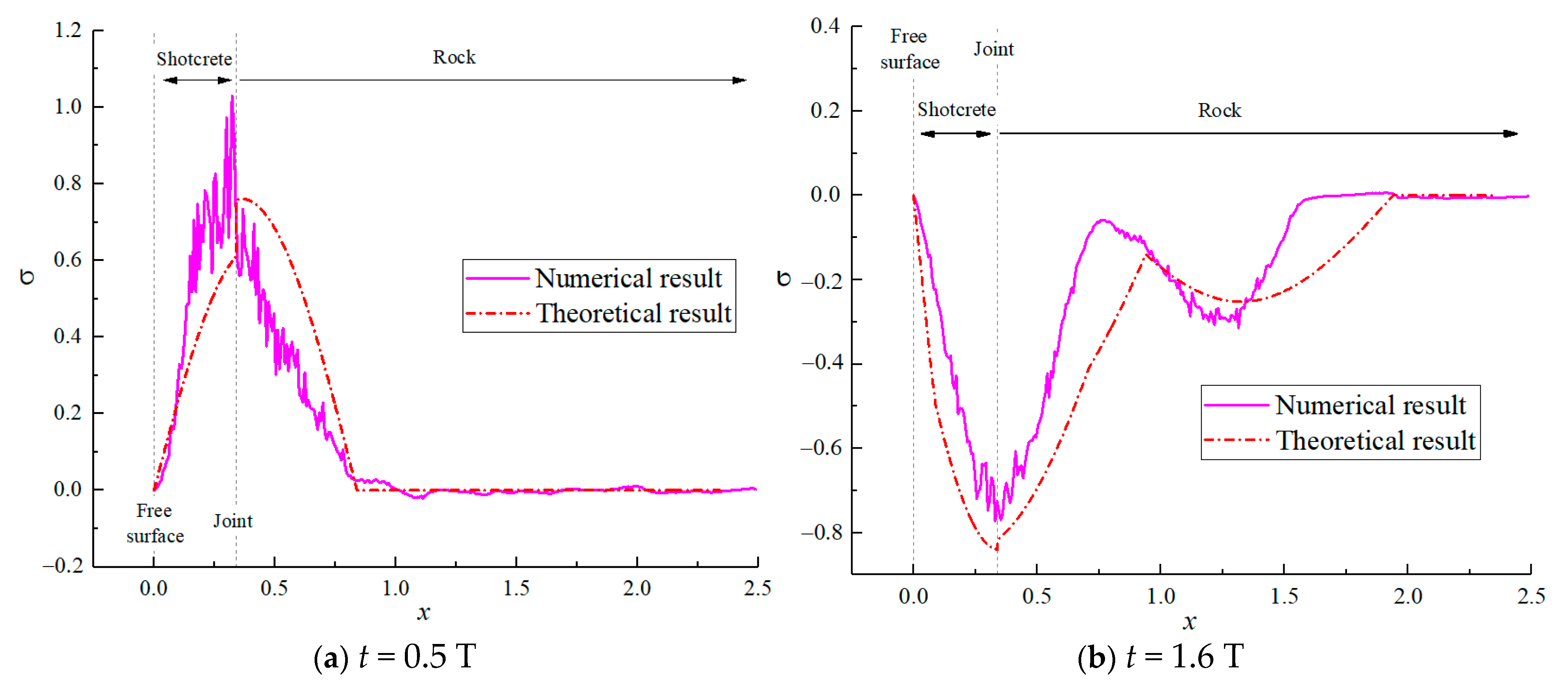
4.2. Stress Evolution Characteristics

As described in Section 2, the stress history at any point in the rock–shotcrete combination could be obtained by Equations (23) and (24). To verify the stress wave characteristics of the rock–shotcrete combination, an incident wave with an amplitude of 10 MPa and a period of 175 μs was applied to the left end of model A. The material parameters of group 1 were selected. In this case, the parameters f₁, f₂, f₃, f₄, P₁, and P₂ were first determined based on Figure 8. Then, the stress components in Formulas (23) and (24) were modified by Formulas (25)–(27). Finally, a MATLAB code was used to invert Formulas (23) and (24), and the stress values corresponding to different positions (x) and different times (t) could be calculated.

Figure 9 shows the variations in stress at points A (L_A = 0.2ηλ_B and 0.4ηλ_B) and B (L_B = 0.7ηλ_B and 0.9ηλ_B) over time. We observed that the numerical waveforms were similar to the theoretical waveforms as a whole with a slight difference in amplitude and time. As shown in Figure 9, the stress amplitude of points A and B decreases with time and gradually approaches zero. Based on Equations (9), (23), and (24), by setting the time t as a constant and location x as an independent variable, the stress distribution of the rock–shotcrete bar at a specific time can be obtained. Furthermore, the location x = 0 represents the free surface. Considering time t = 0.5 T and 1.6 T as examples, the stress distribution of the rock–shotcrete bar is presented in Figure 10. Although slight differences were present in amplitude and time, we observed the stress–location curves were similar between the numerical and theoretical results. In addition, we observed that when t = 0.5 T, practically no tensile stress existed in the rock–shotcrete combination, and the compressive stress near the joint was the largest. When t = 1.6 T, tensile stress occurred not only in the rock but also in the shotcrete and at the joint. However, the value of tensile stress in the three components was different. Evidently, the maximum tensile stress was distributed near the joint.

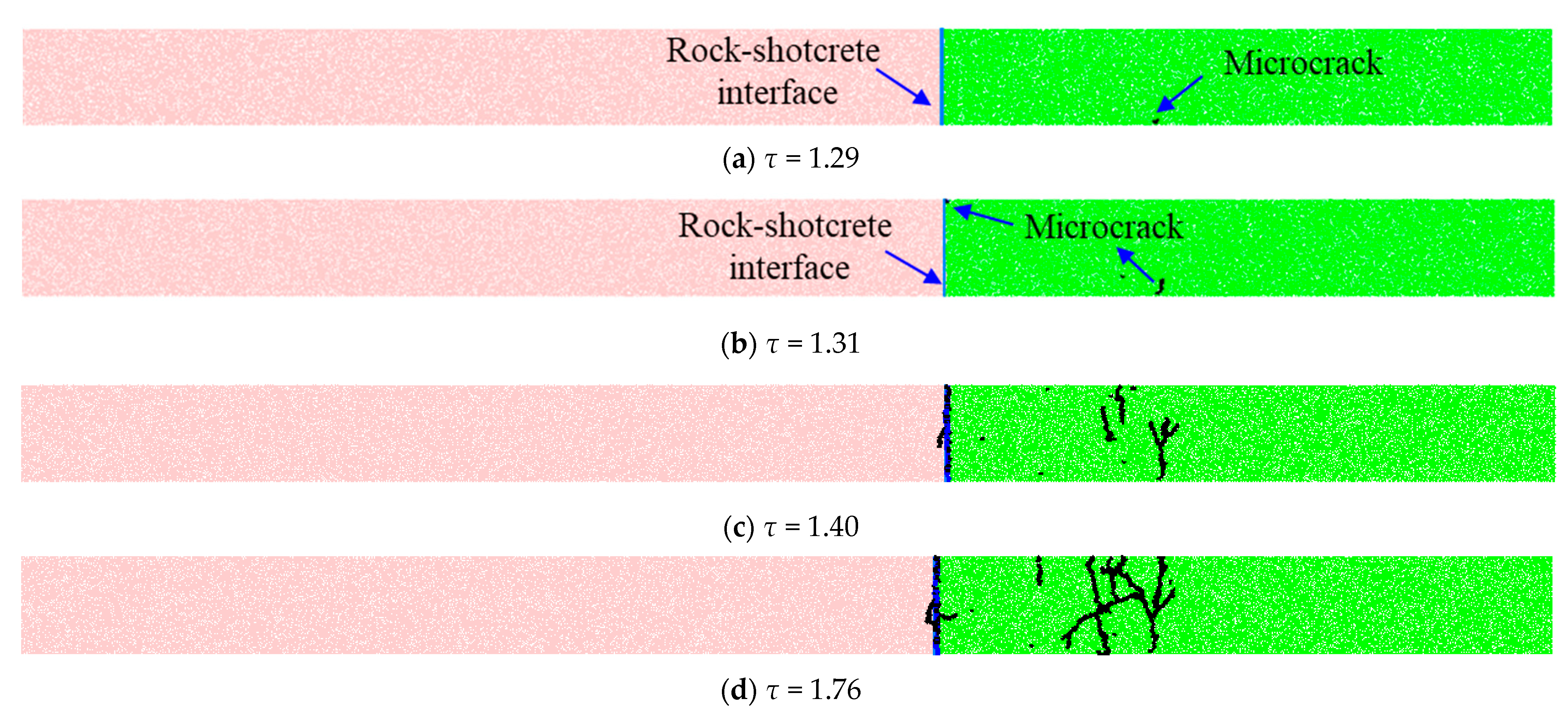
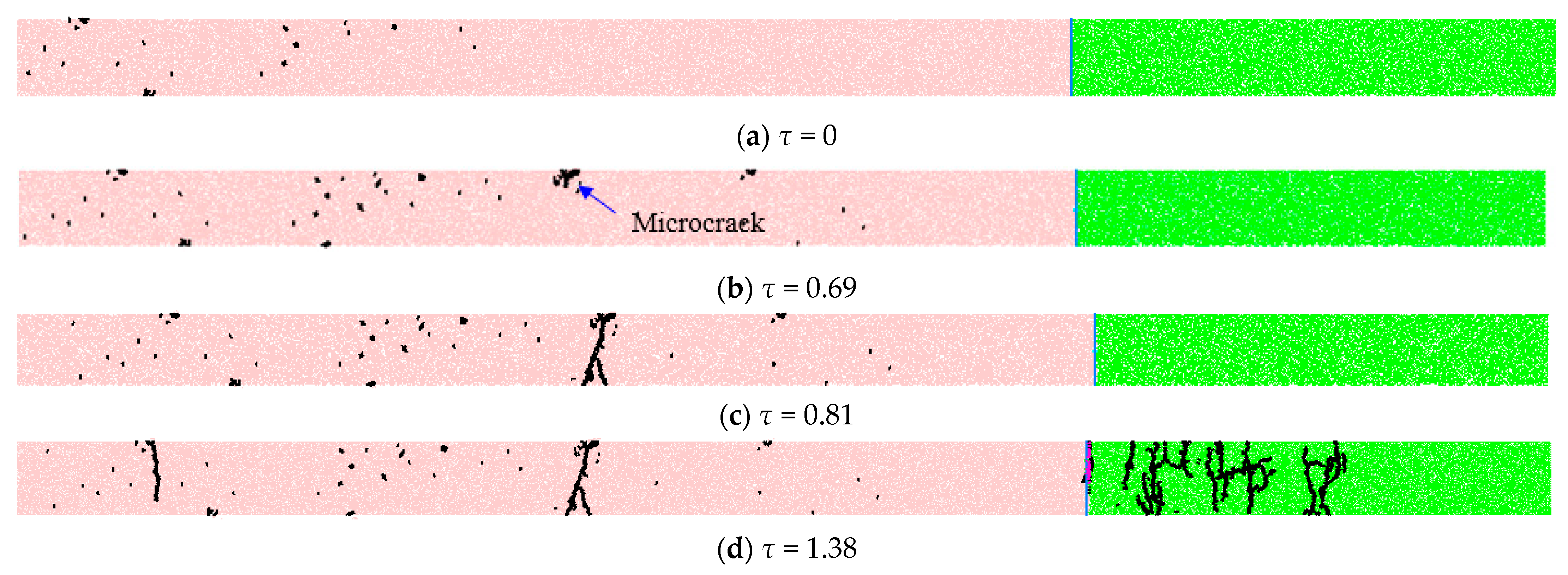
4.3. Spalling Characteristics

As described in Section 3, the location of the initial spalling was related to the normalized tensile strength of the materials. To verify the initial spalling characteristics of the rock–shotcrete combination, model A was applied in this section. Three cases are discussed, and their corresponding simulation schemes are shown in

Table 4. Initial spalling characteristics based on theory and numerical simulation.

Case	Model	Material	Incident Amplitude σm, MPa	Spalling Time, τ		Spalling Location, x
				Theoretical	Numerical	Theoretical	Numerical
Case 1	A	Group 1	15	1.24	1.19–1.23	0.339	0.339
Case 2	A	Group 2	30	1.15	1.29–1.40	0.339	0.339, 0.22
Case 3	A	Group 2	60	0.74	0.69–0.81	0.605	0.69

. As shown in Table 4, both sets of material parameters (group 1 and group 2) were used, and three stress waves with a period of 175 μs and different incident amplitudes (15, 30, and 60 MPa) were considered.

Figure 11, Figure 12 and Figure 13 show three typical spalling cases. It should be noted that the PFC2D 5.0 software provides an external crack insertion program to determine whether micro bonds between particles are damaged. When the stress inside the interparticle bond reaches its strength, the PFC2D software will mark the bond as broken and add a microscopic line at the bond location to indicate microcracks. In this study, this black small line represents newly formed microcracks, and this blue line represents the prefabricated rock–shotcrete interface, as shown in Figure 12. As shown in Figure 11, we observed that when the normalized time τ = 1.19, tensile cracks began to appear at the joint, and afterward, the joint failed at τ = 1.23. Furthermore, no additional damage was detected to the rock and shotcrete. In case 2, the initial spalling occurred practically simultaneously in the shotcrete and at the joint. As shown in Figure 12, at τ = 1.29 T, the shotcrete began to form microcracks, and only after a very short period (Δτ ≤ 0.02), microcracks appeared at the joint. When τ = 1.40 T, the joint completely failed, and a few discontinuous macro spalling cracks were formed in the shotcrete. Afterward, the damage of the shotcrete was increased under the residual stress wave, while the rock remained intact. For case 3, since the amplitude of the incident wave was large enough, a few initial damages occurred in the rock before the incident wave reached the joint for the first time, as shown in Figure 13a. Then, the microcrack in the rock started to expand at τ = 0.69 T, and a macro spalling crack was finally formed at τ = 0.81 T. Afterward, new macro failures appeared in the rock, joint, and shotcrete under the residual stress wave.

By comparing the above three cases, we observed that if the joint strength was small (e.g., case 1), a small incident amplitude (e.g., 15 MPa) could easily cause joint damage. However, if the joint strength was larger (e.g., case 2), a medium incident amplitude (e.g., 30 MPa) was not sufficient to cause the joint and rock to be damaged first. Interestingly, if the loading amplitude continued to increase (e.g., 60 MPa), the reflected wave in the rock first reached its tensile strength. Therefore, spalling first occurred in the rock. The three examples provided a vivid insight into the relationship between the spalling characteristics and incident amplitude along with the strength of the materials. Therefore, the inherent strength of materials and the amplitude of the incident wave might cause various spalling characteristics. Table 4 compares both the theoretical and numerical results of the cases. As shown in Table 4, the numerical results are consistent with the theoretical results in predicting the location and time of initial spalling.

5. Influence of the Thickness of Shotcrete

5.1. Influence of the Thickness of Shotcrete on Stress Evolution

To study the influence of the thickness of shotcrete δ on the stress evolution of a rock–shotcrete combination, four levels of thickness (δ = 0.1ηλ_B, 0.2ηλ_B, 0.5ηλ_B, and 0.8ηλ_B) were designed and input into the MATLAB code to obtain the maximum tensile stress and its corresponding locations, as shown in Figure 14. We noticed that the thickness of shotcrete δ had a significant effect on stress evolution. The stress evolution is characterized as follows:

(a)

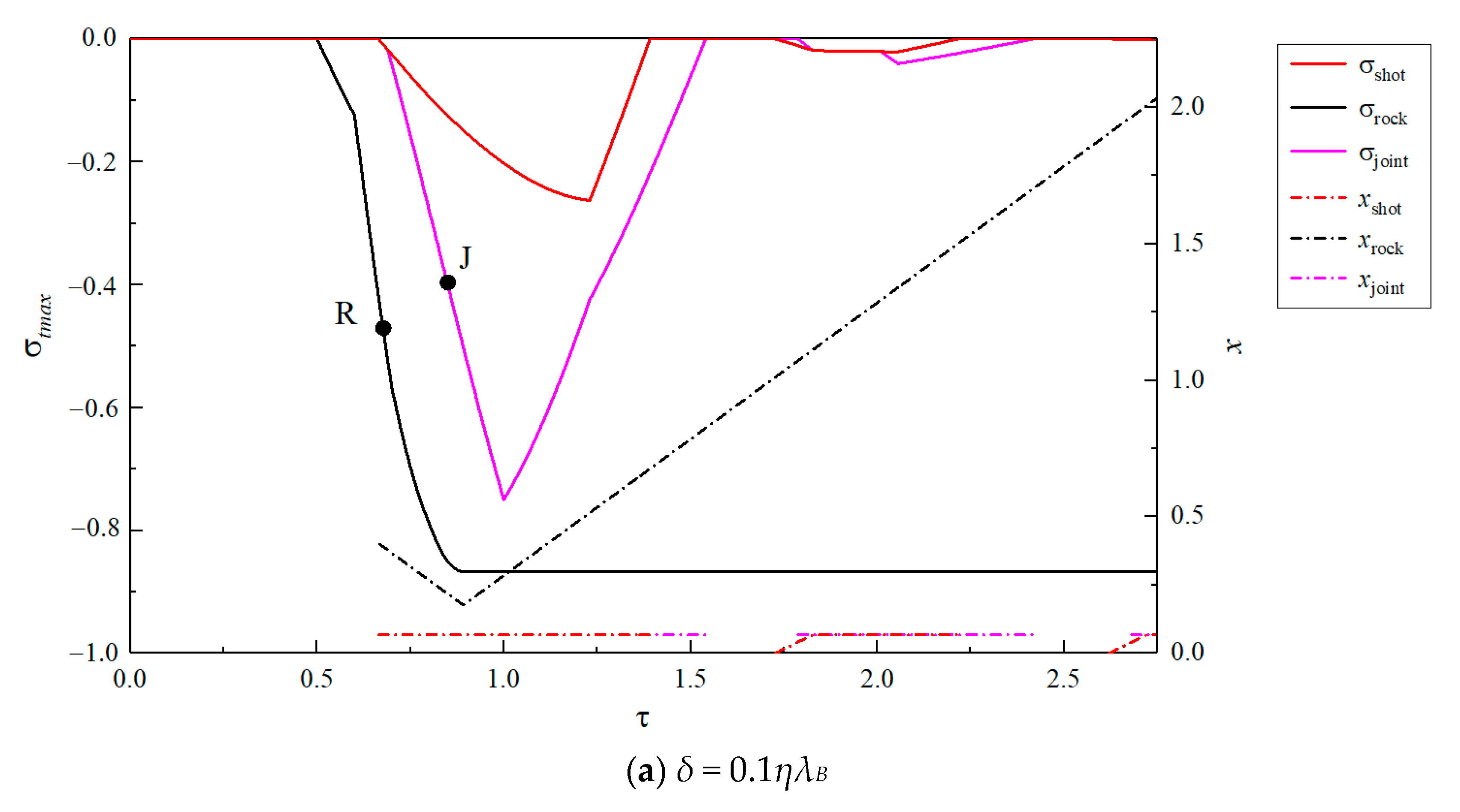
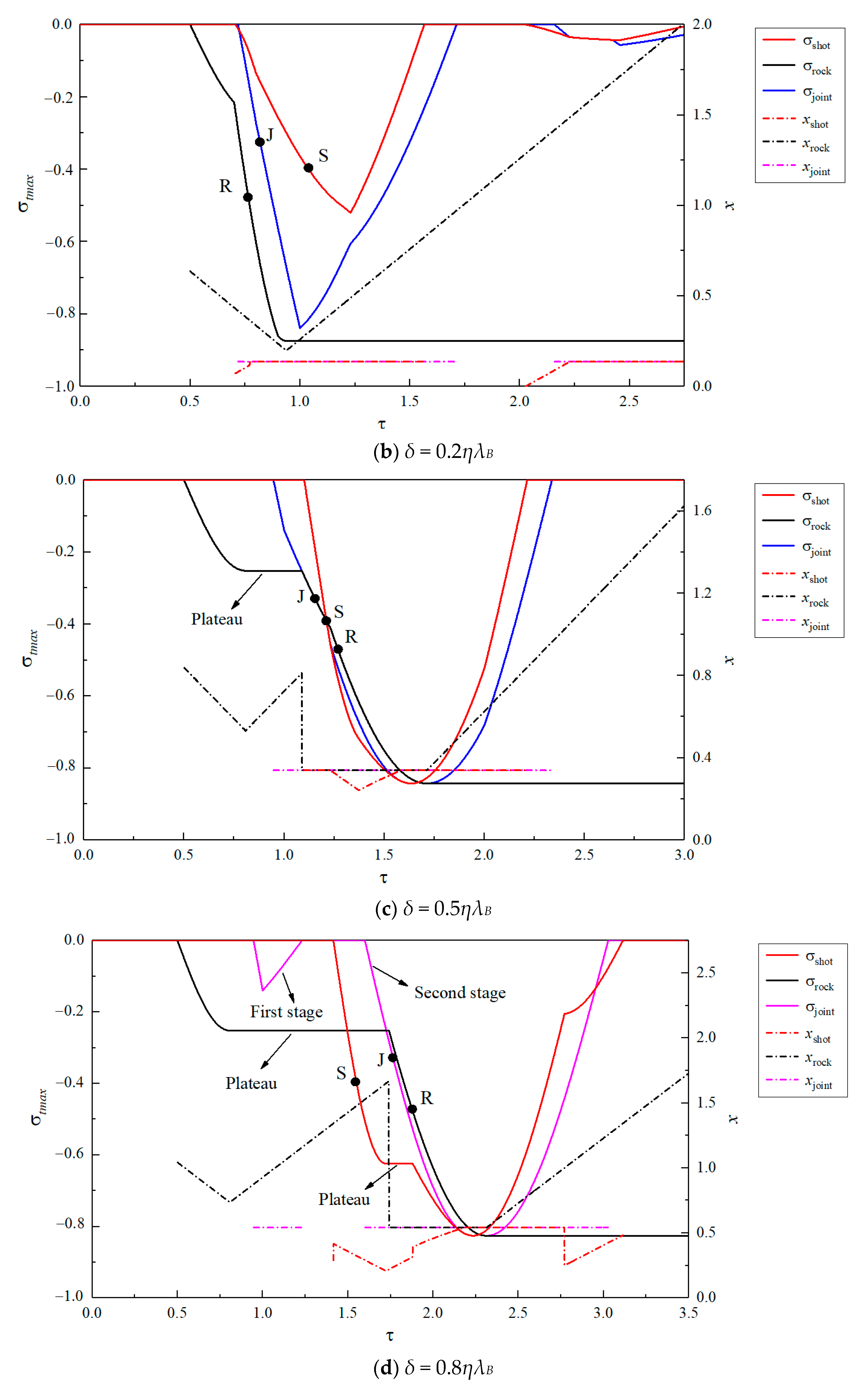
From Figure 14, we observed that the tensile stress always occurred first in the rock, while after a certain time interval, the tensile stress appeared in the shotcrete and at the joint. This result was obtained because the reflected wave in the rock was the tensile stress wave after the incident wave reached the joint for the first time, while in the shotcrete, the transmitted wave was the compressive stress wave. Thus, for generating the tensile stress in the shotcrete, one reflection is required to occur on the free surface at least, and the actual time of the net tensile stress lags behind the reflection time on the free surface due to the superposition effect with the original compression wave. Moreover, if the shotcrete was not long enough, it might take a considerable time for the total stress to change to tensile stress. At the joint, the tensile stress primarily depends on the stress difference between the two sides. In conclusion, for the thin shotcrete (e.g., δ = 0.1ηλ_B and δ = 0.2ηλ_B), the tensile stress at the joint and in the shotcrete appeared practically simultaneously. However, for the thick shotcrete (e.g., δ = 0.5ηλ_B and δ = 0.8ηλ_B), the tensile stress of the joint preceded the shotcrete, as shown in Figure 14.

(b)

For the thick shotcrete (e.g., δ = 0.5ηλ_B and δ = 0.8ηλ_B), there was a plateau in the stress–time curves of rock and shotcrete. However, this phenomenon did not occur in the thin shotcrete (e.g., δ = 0.1ηλ_B and δ = 0.2ηλ_B) because when the shotcrete was thick, it took a long time to generate new stress waves from the joint. Therefore, the original stress waves in the rock and shotcrete propagated stably for a period until the subsequent waves were sufficiently superimposed with them.

(c)

When the thickness was small (e.g., δ = 0.1ηλ_B and δ = 0.2ηλ_B), the tensile stress of the shotcrete was lower than that of the joint, and the tensile stress of the rock was the largest. However, when the thickness was moderate (e.g., δ = 0.5ηλ_B), the peaks of maximum tensile stress of rock, shotcrete, and joint were nearly equal. We noted that when the thickness was large enough (e.g., δ = 0.8ηλ_B), the tensile stress of the joint exhibited two stages: in the first stage, the peak of this maximum tensile stress was small; while in the second stage, the peak of the joint was equal to that of rock and shotcrete.

5.2. Influence of the Thickness of Shotcrete on Spalling Characteristics

In the above section, the influence of shotcrete thickness δ on the stress evolution of a rock–shotcrete bar and its reasons were analyzed. Based on the results, different spall failures might be caused by the change in the thickness of the shotcrete. For example, when the shotcrete δ was sufficiently thin (e.g., δ = 0.1ηλ_B and δ = 0.2ηλ_B), since the tensile stress first appeared in the rock, the rock might initially experience spalling as long as the normalized strength of the rock was appropriate. However, when the thickness of the shotcrete increased to a certain extent, the initial spalling might be transferred to the joint or shotcrete because the tensile stress wave in the rock propagated stably for a period before continuing to increase. Generally, when the thickness of the shotcrete was moderate (e.g., δ = 0.5ηλ_B), the initial spalling was prone to occur at the joint since the tensile stress first occurred at the joint rather than the shotcrete, and the tensile strength of the joint was usually less than that of the shotcrete. However, if the shotcrete was thick enough (e.g., δ = 0.8ηλ_B), the initial spalling might occur preferentially in the shotcrete because it might take a longer time for the tensile stress of the joint to increase to a point at its second stage (as shown in Figure 14d).

Figure 15 shows four spalling cases with different shotcrete thicknesses. The four cases have the same material parameters and loading amplitudes, which could be referred to as case 2 in Table 4. Based on Table 2 and Table 4, the corresponding normalized tensile strength values of the rock, joint, and shotcrete are 0.471, 0.327, and 0.395, respectively, and their theoretical spalling points (R, J, S) are also shown in Figure 14. As shown in Figure 14, points R, J, and S represent the failure points of the rock, joint, and shotcrete, respectively. As shown in Figure 14a, when δ = 0.1ηλ_B, the corresponding time at point R was significantly smaller than that at point J, indicating that the rock might fail before the joint, which was consistent with the numerical results (as shown in Figure 15a). As the tensile stress of the shotcrete is less than its normalized strength of 0.395, point S is not shown in Figure 14a. When δ = 0.2ηλ_B, as shown in Figure 14b, the corresponding time of point R is slightly smaller than that of point J (Δτ < 0.052 T), indicating that failure occurs in the rock slightly earlier than that at the joint. In contrast, in the numerical simulation, the joint was prior to failure, as shown in Figure 15b. When δ = 0.5ηλ_B, as shown in Figure 14c, the spalling of the joint occurs slightly earlier than that in the shotcrete (τ_J < τ_S). However, in the numerical simulation, the spalling of the joint and shotcrete appeared practically at the same time, as shown in Figure 12 and Figure 15c. When δ = 0.8ηλ_B, both theoretical and numerical results indicated that the spalling occurred preferentially in shotcrete (τ_S < τ_J < τ_R), as shown in Figure 14d and Figure 15d.

In summary, the numerical simulation results were consistent with the theoretical analysis. However, a few differences still appeared in the two cases of δ = 0.2ηλ_B and 0.5ηλ_B, and this might be because the microscopic geometrical morphology and mechanical parameters of the numerical materials were not completely homogeneous, while the materials assumed in the theory were completely homogeneous. For example, in the above two cases, the theoretical time interval between the first and second points was very short (Δτ < 0.052 T for δ = 0.2ηλ_B, Δτ < 0.051 T for δ = 0.5ηλ_B). Therefore, a slight error in the material strength or incident amplitude measured by the numerical model might lead to a change in the theoretical initial spalling. Therefore, the suggested theoretical analysis method was generally acceptable. However, sufficient attention should also be paid to the errors, which could cause a mismatch between actual and theoretical parameters. Additionally, the results indicated that the thickness of the shotcrete had a significant effect on the spalling characteristics of the rock–shotcrete combination.

6. Discussion

The propagation of stress waves caused by blasting in a single medium has been widely studied, and some attention has also been paid to two-medium interfaces, for example, by Ma et al. [42]. However, a rock–shotcrete interface is often subjected to dynamic loading caused by adjacent tunnel excavation, which has not received enough attention. The problem is further complicated by the existence of rock–shotcrete interfaces and excavation free surfaces. The propagation and spalling behavior of rock–shotcrete combinations are actually very complex. The basic principle of spalling mainly depends on the material, i.e., rock, shotcrete, or joint, whose tensile stress reaches its spalling strength first. For this, the propagation law of stress waves during rock–shotcrete interface and excavation free surface was analyzed, and a method to predict the location and time of the initial spalling was proposed by comparing the maximum tensile stress inside the rock–shotcrete combination. In this method, determining whether the normalized stress of rocks, joints, and shotcrete is close to the normalized strength is important information for identifying whether spalling occurs. Usually, there are many parameters that affect the normalized stress and strength of the rock, shotcrete, and joint, such as incident wave amplitude, shotcrete thickness, and material tensile strength.

In fact, regardless of the actual dynamic loading conditions (borehole spacing, borehole diameter, etc.), stress waves are the main loads leading to the dynamic failure of rock masses. The amplitude of the incident wave generated by an explosion is the parameter most directly related to explosion energy. Generally, the greater the blasting energy, the greater the damage to the surrounding rock mass and lining. On the other hand, different types of shotcrete production actually affect the tensile strength and elastic modulus of the shotcrete. According to Equation (17), it can be found that increasing the tensile strength of the shotcrete and decreasing the amplitude of the incident wave have similar effects on reducing the risk of spalling of the material. At the same time, different shotcreting techniques may result in varying thickness and roughness of shotcrete. Therefore, it is also very important to explore the changes in the morphological parameters and basic composition changes of shotcrete. For example, Mitelman and Elmo [43] have demonstrated the ineffectiveness of bonded fiber-reinforced liner in resisting intensive blast damage. Zhu et al. [10] found that shotcreting with sufficient thickness could effectively reinforce the surrounding rock and reduce the area of disturbed zones facing dynamic extension.

In this paper, two levels of explosion incident amplitude and four types of shotcrete thickness were designed in the numerical study, and initial spalling failure modes with respect to these two parameters were obtained. As shown in Figure 16, the higher the incident energy is, the thinner the shotcrete is, and the more easily the initial spalling failure occurs in the rock, which is contrary to the original intention of engineers to protect the surrounding rock with shotcrete. Increasing the thickness of the shotcrete and decreasing the incident energy of a single explosion will make the initial spalling failure more likely to occur at the interface or in the shotcrete. Therefore, the amount of explosive in a single charge needs to be strictly controlled during the blasting design. Meanwhile, when shotcrete support is implemented after excavation, it is necessary to control the thickness of the shotcrete. The thickness of shotcrete should not be too thin; it should be at least more than 0.2 times the wavelength of shotcrete. Malmgren et al. [44] also suggested that it is also important to obtain sufficient thickness all over the shotcreted area, i.e., avoid areas with thin shotcrete (20 mm or less), which is in accordance with the results in this paper. However, in further research, Malmgren and Nordlund [45] indicated that the number of failures in the interface increased more than the number of failures in the lining decreased with an increase in shotcrete thickness, which runs counter to the results of this paper. This is mainly because that research was under static conditions, while this paper considers the spalling failure under dynamic loading. It can be seen that the conclusions drawn from static loading conditions and dynamic loading conditions are diametrically opposite. Therefore, when designing shotcrete support, if blasting is adopted in the subsequent excavation, the influence of dynamic load should be fully considered, although the original intention of shotcrete support is only to resist self-weight.

In this paper, the half-sine wave was used to study the dynamic response of rock–shotcrete behavior. However, some other excavation methods in underground engineering may cause different loading conditions, so the spalling behavior and spalling characteristics of rock–shotcrete combinations will differ, and there will be a need to re-determine the nonlinear elastic parameters of the joint and the normalized stress inside the rock–shotcrete combination based on the specific incident waveform.

7. Conclusions

Although shotcrete support is primarily used to control gravity-induced rockfall and manage shallow zones of loose rock, underground engineering with shotcrete lining is always subjected to the disturbance of dynamic loading, such as explosions, which may cause severe spalling failures in surrounding rock or in shotcrete lining. In this paper, based on the stress wave theory, the stress wave propagation and its superposition in a rock–shotcrete combination was analyzed, and a method for predicting the location and time of initial spalling was proposed and described thoroughly. A numerical method was used to study the spalling characteristic of the rock–shotcrete combination and further confirmed that the proposed theoretical method is reliable. In addition, the incident amplitude of the wave and the thickness of the shotcrete have an important effect on the spalling characteristics of a rock–shotcrete combination, especially the initial spalling location and time.

The results show that the spalling characteristics of a rock–shotcrete combination are closely related to the incident amplitude and the thickness of shotcrete. A larger amount of incident energy and thinner thickness of shotcrete will lead to initial spalling failure inside the rock, which is contrary to the original intention of protecting the surrounding rock. However, a lower incident energy and thicker shotcrete thickness will lead to the initial spalling failure occurring inside the shotcrete or at the interface, which may result in the operation of re-shotcrete. The amount of explosive in a single charge needs to be controlled, and too-thin shotcrete should be avoided when spraying. This study provides a theoretical basis and useful guidelines for support performance in tunnel engineering.

References

1. Min, G.; Fukuda, D.; Oh, S.; Cho, S. Investigation of the dynamic tensile fracture process of rocks associated with spalling using 3-D FDEM. Comput. Geotech. 2023, 164, 105825. [Google Scholar] [CrossRef]
2. Wang, S.M.; Wang, J.Q.; Xong, X.R.; Chen, Z.H.; Gui, Y.L.; Zhou, J. Effect of oblique incident wave perturbation on rock spalling: An insight from DEM modelling. J. Cent. South Univ. 2023, 30, 1981–1992. [Google Scholar] [CrossRef]
3. Chen, B.P.; Li, Y.C.; Tang, C.A. Numerical Study on the Zonal Disintegration of a Deeply Buried High-Temperature Roadway during Cooling. Comput. Geotech. 2024, 165, 105848. [Google Scholar] [CrossRef]
4. Qiu, J.D.; Xie, H.P.; Zhu, J.B.; Wang, J.; Deng, J.H. Dynamic response and rockburst characteristics of underground cavern with unexposed joint. Int. J. Rock Mech. Min. Sci. 2023, 169, 105442. [Google Scholar] [CrossRef]
5. Xiao, P.; Liu, H.X.; Zhao, G.Y. Characteristics of ground pressure disaster and rockburst proneness in deep gold mine. Lithosphere 2023, 2022, 9329667. [Google Scholar] [CrossRef]
6. Zhao, R.; Tao, M.; Wu, C.Q.; Wang, S.F.; Zhu, J.B. Spallation damage of underground openings caused by excavation disturbance of adjacent tunnels. Tunn. Undergr. Sp. Technol. 2023, 132, 104892. [Google Scholar] [CrossRef]
7. Jiang, Q.; Feng, X.T.; Chen, J.; Huang, K.; Jiang, Y.L. Estimating in-situ rock stress from spalling veins: A case study. Eng. Geol. 2013, 152, 38–47. [Google Scholar] [CrossRef]
8. Weerheijm, J.; Van Doormaal, J.C.A.M. Tensile failure of concrete at high loading rates: New test data on strength and fracture energy from instrumented spalling tests. Int. J. Impact Eng. 2007, 34, 609–626. [Google Scholar] [CrossRef]
9. Li, X.B.; Tao, M.; Gong, F.Q.; Yin, Z.Q.; Du, K. Theoretical and experimental study of hard rock spalling fracture under impact dynamic loading. Chin. J. Rock Mech. Eng. 2011, 30, 1081–1088. [Google Scholar]
10. Zhu, J.B.; Li, Y.S.; Peng, Q.; Deng, X.F.; Gao, M.Z.; Zhang, J.G. Stress wave propagation across jointed rock mass under dynamic extension and its effect on dynamic response and supporting of underground opening. Tunn. Undergr. Sp. Technol. 2021, 108, 103648. [Google Scholar] [CrossRef]
11. Qiu, J.D.; Li, D.Y.; Li, X.B.; Zhu, Q.Q. Numerical investigation on the stress evolution and failure behavior for deep roadway under blasting disturbance. Soil Dyn. Earthquake Eng. 2020, 137, 106278. [Google Scholar] [CrossRef]
12. Li, X.B.; Tao, M.; Wu, C.Q.; Du, K.; Wu, Q.H. Spalling strength of rock under different static pre-confining pressures. Int. J. Impact Eng. 2017, 99, 69–74. [Google Scholar] [CrossRef]
13. Xie, H.P.; Zhu, J.; Zhou, T.; Zhang, K.; Zhou, C.T. Conceptualization and preliminary study of engineering disturbed rock dynamics. Geomech. Geophys. Geo-Energy Geo-Resour. 2020, 6, 1–14. [Google Scholar] [CrossRef]
14. Si, X.F.; Luo, Y.; Luo, S. Influence of lithology and bedding orientation on failure behavior of “D” shaped tunnel. Theor. Appl. Fract. Mech. 2024, 129, 104219. [Google Scholar] [CrossRef]
15. Li, C.J.; Li, X.B. Influence of wavelength-to-tunnel-diameter ratio on dynamic response of underground tunnels subjected to blasting loads. Int. J. Rock Mech. Min. Sci. 2018, 112, 323–338. [Google Scholar] [CrossRef]
16. Xie, H.P.; Zhu, J.B.; Zhou, T.; Zhao, J. Novel three-dimensional rock dynamic tests using the true triaxial electromagnetic Hopkinson bar system. Rock Mech. Rock Eng. 2021, 54, 2079–2086. [Google Scholar] [CrossRef]
17. Qiu, J.D.; Li, D.Y.; Li, X.B. Dynamic failure of a phyllite with a low degree of metamorphism under impact Brazilian test. Int. J. Rock Mech. Min. Sci. 2017, 94, 10–17. [Google Scholar] [CrossRef]
18. Fan, L.F.; Yang, Q.H.; Du, X.L. Spalling characteristics of high-temperature treated granitic rock at different strain rates. J. Rock Mech. Geotech. 2023, 16, 1280–1288. [Google Scholar] [CrossRef]
19. Martin, C.D.; Christiansson, R. Estimating the potential for spalling around a deep nuclear waste repository in crystalline rock. Int. J. Rock Mech. Min. Sci. 2009, 46, 219–228. [Google Scholar] [CrossRef]
20. Kubota, S.; Ogata, Y.; Wada, Y.; Simangunsong, G.; Shimada, H.; Matsui, K. Estimation of dynamic tensile strength of sandstone. Int. J. Rock Mech. Min. Sci. 2008, 45, 397–406. [Google Scholar] [CrossRef]
21. Zhao, H.T.; Tao, M.; Li, X.B.; Cao, W.Z.; Wu, C.Q. Estimation of spalling strength of sandstone under different pre-confining pressure by experiment and numerical simulation. Int. J. Impact Eng. 2019, 133, 103359. [Google Scholar] [CrossRef]
22. Cho, S.H.; Ogata, Y.; Kaneko, K. Strain-rate dependency of the dynamic tensile strength of rock. Int. J. Rock Mech. Min. Sci. 2003, 40, 763–777. [Google Scholar] [CrossRef]
23. Salem, S.; Eissa, E.; Zarif, E.; Sherif, S.; Shazly, M. Influence of moisture content on the concrete response under dynamic loading. Ain Shams Eng. J. 2023, 14, 101976. [Google Scholar] [CrossRef]
24. Peng, S.; Wu, B.; Du, X.Q.; Zhao, Y.F.; Yu, Z.P. Study on dynamic splitting tensile mechanical properties and microscopic mechanism analysis of steel fiber reinforced concrete. Structures 2023, 58, 105502. [Google Scholar] [CrossRef]
25. Erzar, B.; Forquin, P. An experimental method to determine the tensile strength of concrete at high rates of strain. Exp. Mech. 2010, 50, 941–955. [Google Scholar] [CrossRef]
26. Zhang, J.Y.; Ren, H.Q.; Han, F.; Sun, G.J.; Wang, X.; Zhao, Q.; Zhang, L. Spall strength of steel-fiber-reinforced concrete under one-dimensional stress state. Mech. Mater. 2020, 141, 103273. [Google Scholar] [CrossRef]
27. Ahmed, L.; Ansell, A. Laboratory investigation of stress waves in young shotcrete on rock. Mag. Concr. Res. 2012, 64, 899–908. [Google Scholar] [CrossRef]
28. Ahmed, L. Models for Analysis of Shotcrete on Rock Exposed to Blasting. Ph.D. Thesis, KTH Royal Institute of Technology, Stockholm, Sweden, 2012. [Google Scholar]
29. Luo, L.; Li, X.B.; Tao, M.; Dong, L.J. Mechanical behavior of rock-shotcrete interface under static and dynamic tensile loads. Tunn. Undergr. Sp. Technol. 2017, 65, 215–224. [Google Scholar] [CrossRef]
30. Shen, Y.J.; Wang, Y.Z.; Yang, Y.; Sun, Q.; Luo, T.; Zhang, H. Influence of surface roughness and hydrophilicity on bonding strength of concrete-rock interface. Constr. Build Mater. 2019, 213, 156–166. [Google Scholar] [CrossRef]
31. Zhou, Z.L.; Lu, J.Y.; Cai, X. Static and dynamic tensile behavior of rock-concrete bi-material disc with different interface inclinations. Constr. Build. Mater. 2020, 256, 119424. [Google Scholar] [CrossRef]
32. Qiu, J.D.; Luo, L.; Li, X.B.; Li, D.Y.; Chen, Y.; Luo, Y. Numerical investigation on the tensile fracturing behavior of rock-shotcrete interface based on discrete element method. Int. J. Min. Sci. Technol. 2020, 30, 293–301. [Google Scholar] [CrossRef]
33. Li, X.B. Rock Dynamics Fundamentals and Applications; Science Press: Changsha, China, 2014. [Google Scholar]
34. Wang, L.L. Foundations of Stress Waves; Elsevier: Amsterdam, The Netherlands, 2007. [Google Scholar]
35. Qiu, J.D.; Zhou, C.T.; Wang, Z.H.; Feng, F. Dynamic responses and failure behavior of jointed rock masses considering pre-existing joints using a hybrid BPM-DFN approach. Comput. Geotech. 2023, 155, 105237. [Google Scholar] [CrossRef]
36. Goodman, R.E. Methods of Geological Engineering in Discontinuous Rocks; West Publishing Company: St. Paul, MN, USA, 1976. [Google Scholar]
37. Kulhawy, F.H. Stress-deformation properties of rock and rock discontinuities. Eng. Geol. 1975, 9, 327–350. [Google Scholar] [CrossRef]
38. Gao, K.; Rougier, E.; Guyer, R.A. Simulation of crack induced nonlinear elasticity using the combined finitediscrete element method. Ultrasonics 2019, 98, 51–61. [Google Scholar] [CrossRef]
39. Liu, Y.G.; Xu, S.L.; Xi, D.Y. Dispersion effect of elastic wave in jointed basalts. Chin. J. Rock Mech. Eng. 2010, 29, 3314–3320. [Google Scholar]
40. Langford, J.C.; Diederichs, M.S. Quantifying uncertainty in Hoek–Brown intact strength envelopes. Int. J. Rock Mech. Min. Sci. 2015, 74, 91–102. [Google Scholar] [CrossRef]
41. Long, X.T.; Wang, G.L.; Lin, W.J.; Wang, J.; He, Z.Q.; Ma, J.C.; Yin, X.F. Locating geothermal resources using seismic exploration in Xian County, China. Geothermics 2023, 112, 102747. [Google Scholar] [CrossRef]
42. Ma, Y.C.; Chen, J.X.; Qiu, H.; Zhuang, J.P.; Zhou, L.; Wang, M. Investigation of stress-wave-induced crack penetration behavior at the rock-Ultra-High-Performance Concrete (UHPC) interface. Theor. Appl. Fract. Mech. 2024, 104399. [Google Scholar] [CrossRef]
43. Mitelman, A.; Elmo, D. Analysis of tunnel support design to withstand spalling induced by blasting. Tunn. Undergr. Sp. Technol. 2016, 51, 354–361. [Google Scholar] [CrossRef]
44. Malmgren, L.; Nordlund, E.; Rolund, S. Adhesion strength and shrinkage of shotcrete. Tunn. Undergr. Sp. Technol. 2005, 20, 33–48. [Google Scholar] [CrossRef]
45. Malmgren, L.; Nordlund, E. Interaction of shotcrete with rock and rock bolts—A numerical study. Int. J. Rock Mech. Min. Sci. 2008, 45, 538–553. [Google Scholar] [CrossRef]
Figure 1. Typical spalling phenomenon in tunnels. (a) Spalling in surrounding rock in Kaiyang Phosphate Mine [6]; (b) spalling in shotcrete in Chambishi copper mine, Zambia; (c) spalling at rock–shotcrete interface in Heiniudong copper mine, China.
Mathematics 12 01346 g001
Figure 2. Typical spalling problem in engineering practice.
Mathematics 12 01346 g002
Figure 3. Propagation process of stress wave in rock–shotcrete combination.
Mathematics 12 01346 g003
Figure 4. Half-sine stress wave propagates along the rock bar with shotcrete.
Mathematics 12 01346 g004
Figure 5. Comparison of stress wave propagation characteristics in linear and nonlinear elastic joints.
Mathematics 12 01346 g005
Figure 6. Variations in the maximum tensile stress and its corresponding location over time: (a) rock; (b) shotcrete; (c) joint.
Mathematics 12 01346 g006
Figure 7. Schematic diagram of numerical model.
Mathematics 12 01346 g007
Figure 8. Comparison of incident waves with transmitted and reflected waves.
Mathematics 12 01346 g008
Figure 9. Variations in stress at points A and B over time.
Mathematics 12 01346 g009aMathematics 12 01346 g009b
Figure 10. Stress distribution of rock–shotcrete bar when t = 0.5 T and 1.6 T.
Mathematics 12 01346 g010
Figure 11. Spalling characteristics of case 1.
Mathematics 12 01346 g011
Figure 12. Spalling characteristics of case 2.
Mathematics 12 01346 g012
Figure 13. Spalling characteristics of case 3.
Mathematics 12 01346 g013
Figure 14. Variations in the maximum tensile stress and its corresponding locations under different thicknesses of shotcrete.
Mathematics 12 01346 g014aMathematics 12 01346 g014b
Figure 15. Spalling characteristics of rock–shotcrete bar with different thicknesses of shotcrete.
Mathematics 12 01346 g015
Figure 16. Typical spalling failure modes in rock–shotcrete combination.
Mathematics 12 01346 g016