Abstract
Querying the geodesic distance field on a given smooth surface is a fundamental research pursuit in computer graphics. Both accuracy and smoothness serve as common indicators for evaluating geodesic algorithms. In this study, we argue that ensuring that the norm of the triangle-wise estimated gradients is not larger than 1 is preferable compared to the widely used eikonal condition. Inspired by this, we formulate the geodesic distance field problem as a Quadratically Constrained Linear Programming (QCLP) problem. This formulation can be further adapted into a Quadratically Constrained Quadratic Programming (QCQP) problem by incorporating considerations for smoothness requirements. Specifically, when enforcing a Hessian-energy-based smoothing term, our formulation, named QCQP-Hessian, effectively mitigates the cusps in the geodesic isolines within the near-ridge area while maintaining accuracy in the off-ridge area. We conducted extensive experiments to demonstrate the accuracy and smoothness advantages of QCQP-Hessian.
MSC:
65D18
1. Introduction
Let, be a smooth 2-manifold surface in 3D, and (or simply without ambiguity) be the distance field defined on rooted at the source point s. The eikonal equation is widely used to characterize a geodesic distance field. This implies that as the destination point moves away from the source point, must change at a rate of “one meter per meter”. As a fundamental research problem in computer graphics and computational geometry, the fast and accurate estimation of geodesic distances [1] is central to various applications. These applications range from surface sampling, parametrization, and skinning [2,3,4] to shape segmentation, registration, and editing [5,6]. Geodesic distance estimation can also be applied in image descriptors [7] and facial action unit recognition [8].
There is a substantial body of literature [9,10,11,12,13,14,15] on computing geodesic distances on polygonal meshes. Some methods are exact if numerical computation is precise [9,10,11,12], while others are approximate [13,14,15]. Run-time performance and accuracy are two key criteria for evaluating geodesic algorithms. It is well-known that an exact geodesic distance field, even on a smooth surface is not smooth everywhere. In certain application scenarios, such as segmentation, intrinsic shape signature, and parameterization [16], there is a desire to compute smooth distances. Since an exact geodesic distance field cannot be smooth on general 3D surfaces, one may need to sacrifice accuracy for smoothness. Representative methods for computing smooth distances on 3D surfaces include commute distances [17], diffusion distances [18], biharmonic distances [19], heat distances [14], and quasi-geodesic distances (QGDF) [20].
However, achieving a trade-off between accuracy and smoothness is seemingly straightforward but highly non-trivial. Despite the ability of the mentioned approaches to produce a smooth distance field, they tend to be weak in predicting an accurate distance field. As the properties of a geodesic distance field have been comprehensively studied in the research community, is non-differential at destination points with two or more shortest paths; these points are referred to as “ridge” points. All the non-differential points form a one-dimensional curve that reveals the topology of the base surface, known as a “ridge” curve. To carefully maintain a balance between accuracy and smoothness, the key for the target distance field is required to be as close as possible to the accurate distance field at off-ridge points. Simultaneously, it should better manifest smoothness than around the ridge curve.
In this paper, we first systematically discuss the behaviors of in both continuous and discrete settings. Let, t be a triangle, and be the exact geodesic distances at the three vertices. Define as the estimated gradients based on . We observe that with the increasing mesh resolution, for triangles located in the off-ridge area (except for just a few triangles incident to the source vertex or pseudo-source vertex). However, for triangles across the ridge curve. This interesting observation implies that can better characterize a geodesic gradient field than the widely used eikonal condition . Recall that the heat-based geodesic method forcibly normalizes to a unit vector, which accounts for the inaccuracy of the heat-based geodesic method in the near-ridge area (we shall validate this observation in Section 4).
In fact, the inequality can be rewritten as a quadratic inequality. All these inequalities collectively define a system of constraints that must satisfy. We further define the objective function as (similar to [20]) and thus formulate the geodesic distance field problem into a Quadratically Constrained Linear Programming (QCLP) problem. Experimental results demonstrate that the QCLP formulation is even more accurate than the well-known fast marching method. Building upon QCLP, we introduce a Hessian-energy-based smoothing term, adapting QCLP into a Quadratically Constrained Quadratic Programming (QCQP). Our extensive experiments show that the QCQP-Hessian formulation effectively mitigates cusps in the geodesic isolines within the near-ridge area while maintaining accuracy in the off-ridge area.
Our contributions are threefold:
- We systematically discuss the behaviors of in both continuous and discrete settings and observe that can better characterize a geodesic gradient field than the eikonal condition .
- We demonstrate that naturally implies the triangle inequality and can produce a distance field that is not larger than that generated by Dijkstra’s algorithm.
- We propose a convex QCLP formulation with a linear objective function and further adapt QCLP to QCQP-Hessian. The latter can eliminate cusps in the geodesic isolines within the near-ridge area while maintaining accuracy in the off-ridge area.
2. Related Works
There is a substantial body of literature on geodesic computation. Existing algorithms encompass both exact and approximate methods, with approximation algorithms further categorized based on differences in algorithmic paradigms. In this section, we initially review exact geodesic algorithms, followed by an exploration of graph-based approximation algorithms. Subsequently, we summarize approximation algorithms based on . Finally, we delve into a review of smoothness-driven algorithms and discuss the objectives of this paper.
2.1. Exact Geodesic Distance Field
When dealing with a surface with an analytic representation, the inquiry of a geodesic path can be formulated as the Euler–Lagrange partial differential equation in differential geometry. However, the PDE generally lacks a closed-form solution, necessitating the use of numerical methods to find a solution.
Considering that a smooth surface can be discretized into a polygonal mesh, researchers initiated the study of computing an exact geodesic distance field on a polygonal surface forty years ago. Representative algorithms include the MMP algorithm [9], the CH algorithm [10], and some variant versions [11,12,21,22,23]. These algorithms commonly utilize a window to encode geodesic paths that share the same edge sequence, allowing for the representation of infinite geodesic paths with a finite number of discrete windows. The key idea is to propagate a dynamic outward wavefront across mesh faces in a Dijkstra-like sweep. Later, the Geodesic Source Propagation (GSP) method [24] is introduced, relying on the propagation of virtual sources. The algorithm distinguishes itself by replacing the traditional priority queue with a dual queue system based on two FIFO queues and adopting an organized cache-coherent mesh layout, thereby enhancing performance. This design makes GSP notable for its outstanding runtime efficiency and accuracy. In contrast to traditional approximation algorithms, GSP has the capability to provide mostly exact distance values, given the correct identification of edge sequences. However, exact geodesic algorithms face challenges in extension to other geometric domains, such as point clouds or tetrahedral meshes.
2.2. Graph-Based Geodesic Distance Approximation
Graph-based methods address the discrete geodesic problem by transforming the polygonal mesh M into a dense graph G, allowing any geodesic path on the mesh M to have an approximate counterpart encoded by G. Aleksandrov et al. [25] propose adding a logarithmic number of Steiner points along each edge of the mesh, placed in a geometric progression along an edge. The computation of a -approximation geodesic path then takes time, where m is the total number of Steiner points, and n is the number of mesh edges. Xin et al. [15] suggest adding m uniformly distributed auxiliary points on the mesh surface, requiring time to construct G with edges. With the help of G, the approximate geodesic distance between any pair of points (not necessarily mesh vertices) can be queried in constant time. Ying et al. [26] propose a saddle vertex graph (SVG) for encoding all-pair geodesic distances. Constructing SVG takes time, where K is the maximal degree to define the proximity between saddle vertices. Wang et al. [27] introduce a discrete geodesic graph (DGG) to approximate the geodesic distance between a pair of points with a specified accuracy, running in empirically linear computational time.
2.3. Approximation Algorithms Based on
Most PDE-based methods aim to solve the Eikonal equation with the boundary condition , where s represents the source point. For instance, the fast marching method (FMM) [13,28,29] employs an upwind finite difference scheme to approximate the accurate geodesic distance field in time. Weber et al. [30] proposed an -time parallel FMM on geometry images. Other approaches solve the Eikonal equation indirectly. For example, the heat method [14], along with its parallel implementation [31], leverages the observation that the heat field and the geodesic distance field share common isolines (though their values may differ). They need to normalize the gradient field into a unit vector field before reconstructing the distance field. The implementation can be found in libigl [32].
2.4. Smoothness Driven Geodesic Algorithms
While there are smoothness-driven geodesic algorithms like commute distances [17], diffusion distances [18], biharmonic distances [19], heat distances [14], and QGDF [20], few studies systematically discuss the relationship between smoothness and accuracy. A geodesic distance field differs significantly from a general scalar field. The distinction lies in the fact that an exact geodesic distance field is naturally smooth at non-ridge points but not at ridge points. To carefully maintain the balance between smoothness and accuracy, the smoothing effect should be enforced in the near-ridge area rather than across the entire surface, which is the goal of this paper.
3. Formulation
In this section, we begin by reviewing the properties of a geodesic distance field . Following that, we delve into the geometric behaviors of in both continuous and discrete settings. Based on this discussion, we enumerate a family of optimization-driven formulations characterized by a linear objective function with various smoothness terms and linear/quadratic constraints.
3.1. Geodesic Distance Field in the Continuous Setting
Given a 2-manifold surface and a source point , there exists a shortest path for any destination point p. Consequently, every point has the shortest distance, forming the continuous geodesic distance field for . The most significant characteristic of a geodesic distance field can be characterized by the famous eikonal equation:
subject to the boundary condition . Intuitively, the eikonal equation states a simple fact: as the destination point moves away from the source, the distance function must change at a rate of “one meter per meter”, as shown in Figure 1.
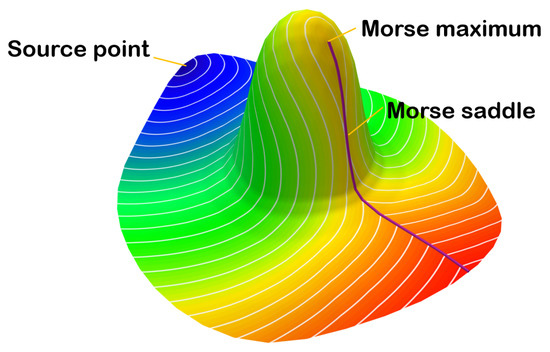
Figure 1.
The gradients of a continuous geodesic distance field are unit everywhere except at the source point and ridge points. Only source points can be Morse-minimum points. The ridge curve is highlighted in purple. Morse-maximum points and Morse-saddle points must lie on the ridge curve.
However, is not differentiable everywhere, even for smooth surfaces. Specifically, if p has only one shortest path to s, then is smooth at p, and holds. However, when there are two or more shortest paths between p and s, is not smooth at p, making it non-differentiable at p. All non-differentiable points form a curve on the surface, called a “ridge”, which characterizes its topology. Polygonal meshes, being piecewise smooth, also exhibit such properties.
According to Morse theory, we make the following observations:
- The source point is the unique Morse-minimum point of the geodesic distance field.
- Each off-ridge point (except the source point) is a Morse-regular point.
- The Morse-maximum points and Morse-saddle points are located on the ridge curve (but not vice versa).
3.2. Unit Gradient and Triangle Inequality
Polygonal meshes are the most prevalent discrete geometric domain for geometry processing. A common practice for encoding a geodesic distance field on a polygonal surface is to compute distance values only at vertices, while the change inside a triangle is considered to be linear. Under this assumption, the gradient is a piecewise constant vector field.
Consider a triangle . Let , , and be the three edge vectors of t. One can estimate the gradient in t based on the distance values , and of the three vertices of t,
where A is the area of t and ⊥ denotes counterclockwise rotation.
Theorem 1.
Let, be one of the triangles in the polygonal mesh . is computed according to Equation (2). If the gradient satisfies , holds and for arbitrary source point.
Proof.
Since the gradient is computed based on the assumption that is linear in t, We have
which implies based on the given condition . □
Theorem 1 demonstrates that by enforcing , the distance field naturally satisfies the triangle inequality property.
3.3. Piecewise Constant Gradient
Now, we assume that is a vector of size n containing all the exact distances at vertices, where n is the number of vertices. When we use the term “exact”, we refer to the path that is the shortest among all those permitted to pass through both edge interior points and face interior points (rather than constrained only to mesh edges). Next, we will provide an in-depth discussion on piecewise constant gradient approximation. Specifically, we will analyze the length of in every triangle. Figure 2 shows the estimated gradients based on Equation (2). In the following, we consider three situations.
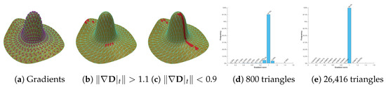
Figure 2.
Triangle-range gradient estimation. (a) By estimating gradients triangle by triangle, we obtain a piecewise constant gradient field. (b) The highlighted triangles are with . (c) The highlighted triangles are with . (d) Most of the triangles satisfy . Among 800 triangles, there are 766 triangles whose gradient norm is between 0.9 and 1.1. (e) Increasing the mesh resolution may increase the proportion of . For example, with 26,416 triangles, 99.3% triangles have unit-length gradients.
- Situation #1:
Suppose that is the source vertex of the triangle . Since encodes the exact geodesic distances at vertices, we have , and . According to
we have
which implies since is a unit vector, and “=” holds only when the vector is co-linear with the edge . Similarly,
also implies , where “=” holds when is co-linear with the edge . Combining the above observations, we have (“=” cannot hold) for the triangles incident to the source vertex. The reason why seems counter-intuitive lies in that , as an approximation of the gradients in t is estimated based on the three distances , and , rather than the change of real geodesic distance in a sufficiently small neighborhood. At the same time, we must point out that may also occur on triangles near the source point or a pseudo-source (although the number of such triangles is quite limited). In Figure 2b, the model consists of 800 triangles, and only seven of them satisfy . When the sparse model is subdivided into a denser version (a total of 26,416 triangles), it has only four triangles with .
- Situation #2:
From Figure 2a, it can be observed that the isolines are fair and equally spaced, without any cusps, in the area away from the source point and the ridge curve. Therefore, the distance propagates approximately “one meter per meter” in such an area, i.e., is roughly a unit vector. Statistics reveal that when the exact geodesic distance of every vertex is available, the gradient length inferred by Equation (2) falls in the range of for 766 triangles (recall that the total number of triangles is 800), indicating that the vast majority of triangles satisfy . When the model is subdivided from 800 triangles into 26,416 triangles, the proportion of triangles with estimated gradients close to 1 in length is further increased.
- Situation #3:
Some triangles are passed through by the ridge curve where geodesics converge from different directions, and the real distance field is far from being linear. If we estimate the gradients in a triangle t using Equation (2), the length of may be far less than 1. In Figure 2c, there are 27 triangles (out of a total of 800) satisfying . In contrast, the denser version (26,416 triangles) has 105 triangles with . Most of these triangles are intersected by the ridge curve. Therefore, the number of such triangles cannot be negligible. At the same time, we must emphasize that may also occur when a large triangle exists (which may not be intersected by the ridge curve); see the left part of Figure 2c.
- Summary
In fact, we can understand the triangle-range gradient estimation from the perspective of divergence:
- If , the triangle-based gradient estimation tends to report .
- If , the triangle-based gradient estimation tends to report .
- If , the triangle-based gradient estimation tends to report .
We plot the histograms of the gradient lengths for the sparse and dense versions of the Hat model; see Figure 2d,e. Based on the statistics, we make the following observations:
- If we estimate the gradients triangle by triangle, the number of triangles satisfying will decrease as the mesh resolution increases.
- There are still many triangles with around the ridge curve, even when the model has a dense triangulation.
- Quadratic constraints
It is reasonable to require the length of to be at most 1 for those triangles not incident to the source vertex, i.e.,
or equivalently
where is a semi-positive-definite matrix (with an eigenvalue of 0), making the quadratic constraint to be convex.
3.4. Geodesic Distance Field on a Graph
Given a graph and a source node , the geodesic distance field on can be computed by querying the minimum distance from s to all the destination vertices in V. In fact, the problem of computing the unknown can also be formulated as standard linear programming [33].
subject to
and
Note, that can also be replaced by a combination:
Since the objective function (9) encourages the disparity between distance values, we call it stretching term in this paper.
Lemma 1.
Proof.
The shortest distances computed by Dijkstra’s algorithm satisfy the triangle inequality. In particular, for each edge , we have
Since the solution to (9) maximizes , we have
Notice that Dijkstra’s algorithm has a property that for any vertex ,
which implies
Let be a sufficiently large number such that for any . We can rewrite the objective function (9) into an equivalent form
Equation (15), with the constraint is a typical minimization problem. After solving the minimization problem, we can recover the actual distance by replacing with . It is worth noting that the resulting distance field has no difference from that reported by Dijkstra’s algorithm. Since the objective function (15) tends to spread out the distances to avoid a trivial solution (i.e., ), we call it “stretching” energy.
Theorem 1 implies that as long as is enforced for every triangle, the triangle inequality naturally holds for every mesh edge. In other words, the condition is stricter than the system of inequalities . Therefore, we immediately obtain the following result.
Theorem 2.
Proof.
Let v be an arbitrary vertex other than source s. When Dijkstra’s algorithm terminates, one can backtrace an edge sequence
that encodes the shortest path. It is easy to see
Since and are in the same triangle and
we have
which completes the proof. □
3.5. Smoothness Energy
In recent years, there has been a trend to consider smoothness requirements when computing a distance field. Various types of smooth geodesic distances have been proposed, including commute distance [17], diffusion distance [18], biharmonic distance [19], and heat distance [14]. Among them, heat distance, with a smoothness feature is closest to the real geodesic distance. Cao et al. [20] developed an optimization method with a quadratic objective function and linear inequality constraints, i.e., Equation (12) for defining constraints, Equation (15) for stretching, and Hessian energy for smoothness.
By reviewing the existing literature, it can be found that accuracy and smoothness were often considered as a trade-off, where increasing smoothness appeared to come at the cost of accuracy. However, the relationship between accuracy and smoothness is not merely a trade-off. It is preferable to maintain the distance field as accurate as possible in the off-ridge area while increasing smoothness in the near-ridge area, which is the goal of this paper. In the following, we review three commonly used smoothing energies.
3.5.1. Dirichlet Energy
Dirichlet energy measures the degree to which the scalar field is close to a harmonic field. In the continuous setting, it is defined by . In the discrete setting, it can be computed by summing the squared gradient norms within each triangle, weighted by the triangle areas. In this paper, we normalize it by dividing it by the total area, ensuring that the energy is independent of the model scale.
where T is the face set, is the area of the triangle t, and the piecewise constant gradient can be computed using Equation (2).
Due to its first-order nature, the Dirichlet-like smoothness energy tends to produce good results for the parts close to the source but may yield poor results (e.g., with unevenly spaced isolines) for the parts away from the source.
3.5.2. Laplacian Energy
The (squared) Laplacian energy, in the continuous setting is also a classical smoothness energy. Given a mesh surface , the sparse/symmetric cot-weight matrix can be computed immediately. The discrete Laplacian energy on a polygonal mesh [34] is defined by
where A is the diagonal matrix of mixed Voronoi areas. The discrete Laplacian energy defined above is independent of the model scale.
3.5.3. Hessian Energy
Stein et al. [35] introduced generalized Hessian energy for curved surfaces by extending their earlier work [36]. The Hessian energy is expressed in terms of the covariant one-form Dirichlet energy, the Gaussian curvature, and the exterior derivative. The discrete form is
where and M are, respectively, the discrete gradient operator, the diagonal matrix of triangle areas, the discrete matrix divergence operator, and the discrete mass matrix; See [36] for details. Similarly, the discrete Hessian energy is also independent of the model scale.
3.6. Various Configurations of Formulation
There are various combinations of objective functions and constraints. We summarize them with a unified template:
where the stretching energy is defined in Equation (15), the smoothness energy can be any of Equations (16)–(18), is a parameter for balancing the stretching term and the smoothness term, and denotes either the linear constraints (Equation (12)) or the quadratic constraints (Equation (8)). Setting yields a solution that is as accurate as possible. With the increasing value of , the resulting distance field becomes smoother around ridge curves but still maintains the accuracy requirement to some degree.
In Table 1, we list a total of eight possible combinations for assembling stretching terms, smoothness terms and constraints, where the LCQP-Hessian combination of Equation (10), Equation (15), and Hessian energy is exactly the QGDF approach [20]. We shall compare them in detail and recommend QCQP-Hessian (Equation (12), Equation (15), and Hessian energy) as the preferred combination in Section 4. It is worth noting that all these formulations belong to convex linear/quadratic programming, ensuring the uniqueness of the solution; in cases where multiple solutions exist, they yield the same value for the objective function.

Table 1.
Eight possible combinations for assembling stretching terms, smoothness terms, and inequality constraints.
4. Evaluation
4.1. Experimental Setting
4.1.1. Experimental Platform and Data Sets
We conducted the experiments on a platform with a 2.8 GHz Intel Core i5-8400 CPU (Intel, Santa Clara, CA, USA) and Win10 operating system. Our algorithm was implemented in Matlab 2020b and Mosek 9.1.9. Some 3D models are commonly used in the graphics community, while others are courtesy of Thingi10k 3D shape repository [37], which contains a large number of anisotropic meshes.
4.1.2. Methods
We include the following geodesic approaches for comparison:
- The VTP algorithm [23] that is a state-of-the-art exact algorithm;
- Dijkstra’s algorithm [38] is a textbook algorithm for computing the shortest paths on graphs.
- The fast marching method [13] is very popular in geodesic approximation;
- The heat-based method [14] can report a smooth distance field in a very short time.
- Quasi geodesic distance field (QGDF) [20] formulates the geodesic distance field problem into a linearly constrained quadratic programming.
Note, that the Geodesic Source Propagation (GSP) method [24] relies on the propagation of virtual sources, distinguishing itself from traditional approximation algorithms. GSP can be considered as a simplified version of exact algorithms. Additionally, in this paper, our goal is to find an algorithm that satisfies both accuracy and smoothness requirements simultaneously. Consequently, we have excluded GSP from our comparisons.
4.2. Ablation Study
4.2.1. QCLP v.s. LCLP
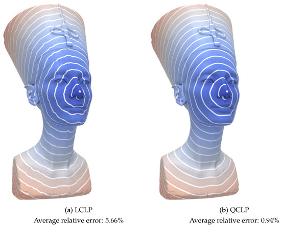
In this paper, we discuss two types of constraints. The first involves enforcing the triangle inequality for each mesh edge, expressed as , where denotes a mesh edge (refer to Equation (12)). The second constraint is to limit the gradient norm to not exceed 1, as indicated in Equation (8). Specifically, Equation (12) characterizes graph-based distance constraints, assuming each path traverses a sequence of mesh edges. In contrast, Equation (8) permits a path passing through face interior points. The constraints defined by Equation (8) are superior to those of Equation (12). In Figure 3, we compare LCLP and QCLP, both having the same objective function but with different constraints. The ablation study reveals that Equation (8) results in a much more accurate distance field than Equation (12), attributed to the requirement of the gradient norm not exceeding 1. Consequently, we recommend QCLP for the accurate estimation of the geodesic distance field and further utilize it to define a smoothness-oriented variant named QCQP-Hessian.
4.2.2. Choice of Smoothness Term
Seeking a smooth distance field is not a simple task. A casual design of the smoothness term can make it challenging to maintain a balance between accuracy and smoothness. Specifically, our aim is to reduce the cusps of the geodesic isolines while keeping the isolines equally spaced in the off-ridge area. We pursue this goal by activating the smoothness term in Equation (19). In Figure 4, we set to different values (e.g., , , , ) and observe the accuracy statistics of the Dirichlet energy, the Laplacian energy, and the Hessian energy. The results indicate that the Hessian smoothness energy is the best choice for preserving accuracy. Therefore, we select the Hessian energy for the smoothness purpose.
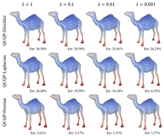
Figure 4.
By setting different values of , we observe that the Hessian smoothness term can better maintain the accuracy.
4.2.3. Ablation Study about
To facilitate users to tune the parameter (independent of model scale and mesh resolution), we take , where n is the number of vertices of the base mesh, h is the average edge length, and m is a user-specified parameter to balance the smoothness and accuracy. Rather than directly finding a suitable , we tune m instead. Based on extensive experimental results, it can be observed that when , the geodesic isolines are approximate with an equal gap and smooth even near the ridge curve, and the cusps of the geodesic isolines are rubbed down as well. But we must point out that users are allowed to specify a different m according to the desired smoothness in practice.
4.2.4. Accuracy with the Increasing Mesh Resolution
In Figure 5, we employ three versions (1K faces, 10K faces, and 100K faces) of the Shell model to assess whether our algorithm improves in accuracy with increasing mesh resolution. The observed reduction in average relative error from 2.53% to 0.57% validates our observation.
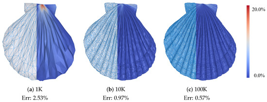
Figure 5.
Our algorithm becomes more and more accurate with the increasing mesh resolution.
4.3. Accuracy Comparison with Existing Algorithms
4.3.1. Subsection Accuracy Comparison on Buddha
We test various algorithms on the 30K-face Buddha model, including Dijkstra’s algorithm [38], the fast marching method [13], the heat method [14], QGDF [20], and our algorithm. We visualize the distribution of relative errors using color coding in Figure 6. Statistics show that the average relative errors of Dijkstra’s algorithm, the fast marching method, the heat method, QGDF, and ours are, respectively, 5.24%, 1.59%, 2.61%, 4.10% and 0.97%. This shows that our algorithm approximates the real geodesic distance field more accurately than the other approximation-based methods. Note, that in practical applications, to maximize the accuracy of our QCQP-Hessian, it is necessary to reduce the weighting coefficient of the Hessian term while increasing it for higher smoothness.
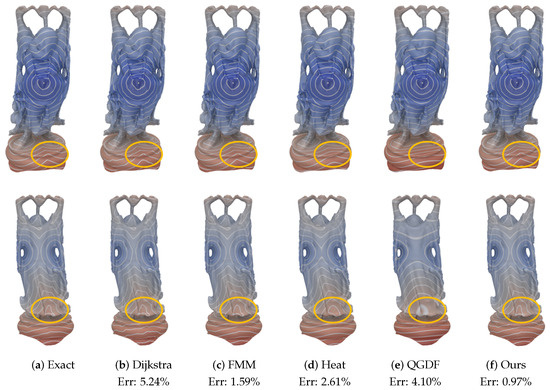
Figure 6.
Visualizing the distribution of relative errors using color coding. The difference can be seen from the highlighted areas. Statistics show that our method is more accurate than most approximation-based methods.
4.3.2. Accuracy Comparison on Anisotropic Meshes
In the field of computer-aided design, there are numerous poorly triangulated models or anisotropic meshes exported from parametric surfaces. It is essential to test if our algorithm can be applied to these models. For a triangle t, one can define the anisotropy measure of t as:
where and S are, respectively, the half-perimeter, the longest edge length, and the area of t. Therefore, the overall anisotropy of a mesh surface can be measured by
where T denotes the face set. We select about 20 models from the Think10K repository whose overall anisotropy scores range from 2 to 50. As Figure 7 shows, the accuracy of Dijkstra’s algorithm, FMM, the heat method, and QGDF decreases on the anisotropic mesh (), but the accuracy of our algorithm (0.21%) remains almost unchanged.
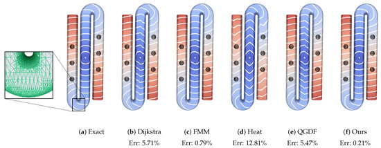
Figure 7.
Our algorithm can report an accurate geodesic distance field on an anisotropic mesh.
4.4. Other Advantages
Capable of Handling Non-Manifold Surfaces
Non-manifold surfaces are also an important kind of geometric domains. For example, medial-axis surfaces, as a compact representation of the original surface are mostly non-manifold. Further reduction in a medial-axis surface into a skeleton needs to analyze the geodesic distance (one can imagine the grassfire transform). Most of the existing geodesic approaches have to depend on half-edge structures in implementation. Recall that our formulation defines the constraints for triangle faces and does not need half-edge structures as the support, which implies that our algorithm is capable of easily handling non-manifold surfaces. We use Figure 8 to show that our algorithm can deal with non-manifold surfaces.
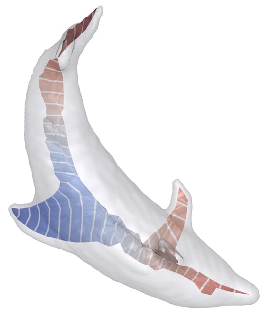
Figure 8.
Our algorithm is capable of easily handling non-manifold surfaces; See the geodesic distance field on the non-manifold medial-axis surface.
4.5. Evaluation on Smoothness
In fact, an exact distance field is generally not smooth, limiting its applicability in some contexts (e.g., defining a shape signature). In recent years, several research works have focused on smoothness-driven distance fields. Representative methods for computing smooth distances include the heat method [14], biharmonic distances [19], and QGDF [20].
In Figure 9, we evaluate these approaches, including ours, on the Bimba model with 51K faces, highlighting differences in the near-ridge area. This example demonstrates that our algorithm achieves better accuracy performance while maintaining smoothness. In detail, the nice features of the QCQP-Hessian formulation are two-fold:
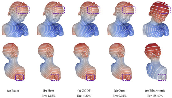
Figure 9.
Comparison with other smooth distance methods: Our algorithm (QCQP-Hessian) slightly refines the cusps of the geodesic isolines while maintaining an approximately equal gap between them. The heat method, on the other hand, tends to over-smooth distances near ridges, leading to larger errors. Refer to the highlighted regions.
- The isolines in the off-ridge area do not vary much with the value of m since the geodesic distance field in the off-ridge area is already very smooth and meets .
- The smoothness term, despite still having a slight effect in the off-ridge area, mainly makes the distance field in the near-ridge area smoother.
To summarize, the requirement of smoothness does not need to be at the cost of accuracy loss.
4.6. Statistics of Accuracy and Run-Time Performance
In Figure 10, we present additional examples generated using our QCQP-Hessian method. We also provide statistics on accuracy and run-time performance for existing approximation-based approaches in Table 2. In terms of accuracy, our approach outperforms other methods. However, in its current form, our algorithm does not have an advantage in terms of run-time performance. This is due to the time-consuming nature of solving quadratic programming, even with Mosek. For instance, our algorithm takes 35.8 s to infer the distance field on the 51K-face Bimba model. In contrast, the exact VTP algorithm runs faster and requires only 0.16 s.
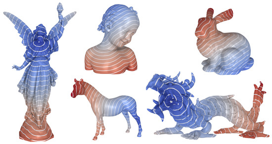
Figure 10.
More results produced by our QCQP-Hessian. The accuracy and run-time performance statistics are shown in Table 2.
Table 2.
Comparison with Dijkstra’s method [39], the fast marching method [13], the heat method [14], the QGDF method [20], and the exact VTP method [23].
4.7. Discussion
4.7.1. Dijkstra’s Algorithm
It is widely employed for computing shortest paths on graphs, thanks to its simplicity and high efficiency. However, traced geodesic isolines using this algorithm may zigzag because the resulting paths are constrained to mesh edges, leading to poor accuracy. Even with a high-resolution input mesh, accuracy cannot be guaranteed. Consequently, it proves ineffective when a high degree of accuracy or smoothness is required.
4.7.2. The Fast Marching Method (FMM)
The FMM achieves asymptotic accuracy when the triangulation of the input mesh is sufficiently dense and of high quality. For a high-resolution mesh, the FMM is a popular and appropriate choice, striking a balance between accuracy and performance. However, the FMM has two main disadvantages. Firstly, it inherits the algorithmic paradigm of Dijkstra’s algorithm, focusing on obtaining an as-accurate-as-possible distance field, without consideration for the smoothness requirement. Secondly, when the input mesh contains skinny triangles, accuracy may decrease, especially for points far from the source, as the propagation-based algorithmic scheme can lead to error accumulation. The key distinction between the FMM and our method is that the FMM propagates distances from near to far, while ours is optimization-driven and independent of the sweeping process. Extensive statistics demonstrate that our algorithm is more accurate than the FMM.
4.7.3. The VTP Algorithm
The VTP algorithm stands out as the most efficient exact geodesic method. It employs a greater number of filtering rules compared to other exact geodesic approaches, and the filtering operation occurs between two windows arriving at the same triangle face but from different bounding edges. However, as it does not consider smoothness, the resulting geodesic isolines may exhibit sharp cusps in the near-ridge area. Therefore, it is not suitable for querying a smooth distance field.
4.7.4. The Heat-Based Method
Crane et al. [14] introduced the heat method (HM), which involves placing heat at the source vertex and diffusing it over a short time to compute the geodesic distance field through the solution of a pair of linear systems. Subsequently, Tao et al. [31] enhanced the speed and scalability of HM but did not address its robustness and accuracy. The primary drawback of HM lies in its accuracy. Our experimental results indicate that the inaccuracy of the heat method arises from two aspects. Firstly, it enforces the gradient norm to be 1 in every triangle, even if the triangle is across the ridge curve, which is less reasonable than . Secondly, the heat method assumes that the isolines of the heat field can align with the isolines of the geodesic distance field (except for misaligned values). However, in numerical implementation, this assumption faces challenges due to poor triangulation and complicated geometry/topology.
4.7.5. The Smooth Quasi-Geodesic Distance Field (QGDF)
Among the existing approximation algorithms, both QGDF and ours are optimization-driven. The distinction lies in the fact that QGDF defines constraints by setting the upper limit of the distance difference for the two endpoints of each mesh edge. If QGDF excludes the smoothness term, it essentially reduces to the graph-based distance field, aligning with the result obtained by Dijkstra’s algorithm. In our QCQP-Hessian approach, we constrain the triangle-based gradients using a set of quadratic inequalities. The theoretical analysis of the differences between them is presented in Section 3.4, where we emphasize that better characterizes a geodesic distance field.
4.7.6. Summary
In this subsection, we compare our geodesic method with other geodesic algorithms in terms of run-time performance, accuracy, and smoothness. The FMM and the heat method exhibit fair accuracy, while Dijkstra’s algorithm performs poorly. Graph-based algorithms, however, come close to providing an exact output. In terms of run-time performance, Dijkstra’s algorithm, the FMM, and the heat method run very fast, whereas graph-based algorithms generally incur a precomputation cost. Regarding smoothness, the heat method and QGDF can produce a smooth distance field, whereas Dijkstra’s algorithm and the FMM cannot. Our QCQP-Hessian approach strikes a balance between accuracy and smoothness requirements simultaneously.
5. Conclusions and Future Work
In this paper, we systematically investigate the gradient of geodesic distances in both continuous and discrete settings. We emphasize that the inequality constraint better characterizes discrete geodesic distances than the widely used eikonal condition . Building on our findings, we propose an optimization-based approach, named QCQP-Hessian, to effectively mitigate cusps in geodesic isolines within the near-ridge area while maintaining accuracy in the off-ridge area. Extensive experimental results validate its effectiveness.
The proposed algorithm, as it currently exists, requires considerable computational resources. With densely triangulated inputs, an effective method to enhance performance involves first applying the algorithm to a simplified version of the mesh. Following this, the generated distance field can then be transferred to the original mesh.
Author Contributions
Conceptualization, S.C. and Y.H.; methodology, N.H.; validation, N.H., S.H. and Z.Y.; formal analysis, N.H.; investigation, S.C.; resources, S.C.; data curation, N.H.; writing—original draft preparation, S.C. and N.H.; writing—review and editing, S.C.; visualization, N.H.; supervision, S.C.; project administration, Y.H.; funding acquisition, S.C. All authors have read and agreed to the published version of the manuscript.
Funding
This research was funded by Natural Science Foundation of China (62002190) and Natural Science Foundation of Shandong Province (ZR2020MF036).
Data Availability Statement
The raw data supporting the conclusions of this article will be made available by the authors on request.
Conflicts of Interest
The authors declare no conflict of interest.
References
- Simon, C.; Koniusz, P.; Harandi, M. On learning the geodesic path for incremental learning. In Proceedings of the IEEE/CVF Conference on Computer Vision and Pattern Recognition, Nashville, TN, USA, 20–25 June 2021; pp. 1591–1600. [Google Scholar]
- Elad, A.; Keller, Y.; Kimmel, R. Texture mapping via spherical multi-dimensional scaling. In Proceedings of the Scale Space and PDE Methods in Computer Vision: 5th International Conference, Scale-Space 2005, Hofgeismar, Germany, 7–9 April 2005; Proceedings 5. Springer: Berlin/Heidelberg, Germany, 2005; pp. 443–455. [Google Scholar]
- Schlömer, T.; Heck, D.; Deussen, O. Farthest-point optimized point sets with maximized minimum distance. In Proceedings of the ACM SIGGRAPH Symposium on High Performance Graphics. ACM, Vancouver, BC, Canada, 5–7 August 2011; pp. 135–142. [Google Scholar]
- Sloan, P.P.J.; Rose, C.F., III; Cohen, M.F. Shape by example. In Proceedings of the 2001 Symposium on Interactive 3D Graphics, Chapel Hill, NC, USA, 26–29 March 2001; ACM: New York, NY, USA, 2001; pp. 135–143. [Google Scholar]
- Rabin, J.; Peyré, G.; Cohen, L.D. Geodesic shape retrieval via optimal mass transport. In Proceedings of the European Conference on Computer Vision, Heraklion, Crete, Greece, 5–11 September 2010; Springer: Berlin/Heidelberg, Germany, 2010; pp. 771–784. [Google Scholar]
- New, A.T.; Mukhopadhyay, A.; Arabnia, H.R.; Bhandarkar, S.M. Non-rigid shape correspondence and description using geodesic field estimate distribution. In ACM SIGGRAPH 2012 Posters; ACM: New York, NY, USA, 2012; p. 96. [Google Scholar]
- Potje, G.; Martins, R.; Cadar, F.; Nascimento, E.R. Learning geodesic-aware local features from RGB-D images. Comput. Vis. Image Underst. 2022, 219, 103409. [Google Scholar] [CrossRef]
- Chen, Y.; Song, G.; Shao, Z.; Cai, J.; Cham, T.J.; Zheng, J. GeoConv: Geodesic guided convolution for facial action unit recognition. Pattern Recognit. 2022, 122, 108355. [Google Scholar] [CrossRef]
- Mitchell, J.S.; Mount, D.M.; Papadimitriou, C.H. The discrete geodesic problem. SIAM J. Comput. 1987, 16, 647–668. [Google Scholar] [CrossRef]
- Chen, J.; Han, Y. Shortest paths on a polyhedron. In Proceedings of the Sixth Annual Symposium on Computational Geometry, Berkeley, CA, USA, 6–8 June 1990; ACM: New York, NY, USA, 1990; pp. 360–369. [Google Scholar]
- Surazhsky, V.; Surazhsky, T.; Kirsanov, D.; Gortler, S.J.; Hoppe, H. Fast exact and approximate geodesics on meshes. ACM Trans. Graph. (TOG) 2005, 24, 553–560. [Google Scholar] [CrossRef]
- Xin, S.Q.; Wang, G.J. Improving Chen and Han’s algorithm on the discrete geodesic problem. ACM Trans. Graph. (TOG) 2009, 28, 104. [Google Scholar] [CrossRef]
- Sethian, J.A. A fast marching level set method for monotonically advancing fronts. Proc. Natl. Acad. Sci. USA 1996, 93, 1591–1595. [Google Scholar] [CrossRef]
- Crane, K.; Weischedel, C.; Wardetzky, M. Geodesics in heat: A new approach to computing distance based on heat flow. ACM Trans. Graph. (TOG) 2013, 32, 152. [Google Scholar] [CrossRef]
- Xin, S.Q.; Ying, X.; He, Y. Constant-time all-pairs geodesic distance query on triangle meshes. In Proceedings of the ACM SIGGRAPH Symposium on Interactive 3D Graphics and Games, Costa Mesa, CA, USA, 9–11 March 2012; ACM: New York, NY, USA; pp. 31–38. [Google Scholar]
- Mejia-Parra, D.; Sánchez, J.R.; Posada, J.; Ruiz-Salguero, O.; Cadavid, C. Quasi-isometric mesh parameterization using heat-based geodesics and poisson surface fills. Mathematics 2019, 7, 753. [Google Scholar] [CrossRef]
- Fouss, F.; Pirotte, A.; Renders, J.M.; Saerens, M. Random-Walk Computation of Similarities between Nodes of a Graph with Application to Collaborative Recommendation. IEEE Trans. Knowl. Data Eng. 2007, 19, 355–369. [Google Scholar] [CrossRef]
- Coifman, R.R.; Lafon, S. Diffusion maps. Appl. Comput. Harmon. Anal. 2006, 21, 5–30. [Google Scholar] [CrossRef]
- Lipman, Y.; Rustamov, R.M.; Funkhouser, T.A. Biharmonic distance. ACM Trans. Graph. (TOG) 2010, 29, 27. [Google Scholar] [CrossRef]
- Cao, L.; Zhao, J.; Xu, J.; Chen, S.; Liu, G.; Xin, S.; Zhou, Y.; He, Y. Computing Smooth Quasi-geodesic Distance Field (QGDF) with Quadratic Programming. Comput.-Aided Design 2020, 127, 102879. [Google Scholar] [CrossRef]
- Liu, Y.J. Exact geodesic metric in 2-manifold triangle meshes using edge-based data structures. Comput.-Aided Des. 2013, 45, 695–704. [Google Scholar] [CrossRef]
- Xu, C.; Wang, T.Y.; Liu, Y.J.; Liu, L.; He, Y. Fast wavefront propagation (FWP) for computing exact geodesic distances on meshes. IEEE Trans. Vis. Comput. Graph. 2015, 21, 822–834. [Google Scholar] [CrossRef]
- Qin, Y.; Han, X.; Yu, H.; Yu, Y.; Zhang, J. Fast and exact discrete geodesic computation based on triangle-oriented wavefront propagation. ACM Trans. Graph. (TOG) 2016, 35, 125. [Google Scholar] [CrossRef]
- Trettner, P.; Bommes, D.; Kobbelt, L. Geodesic Distance Computation via Virtual Source Propagation. In Computer Graphics Forum; Wiley Online Library: Hoboken, NJ, USA, 2021; Volume 40, pp. 247–260. [Google Scholar]
- Aleksandrov, L.; Lanthier, M.; Maheshwari, A.; Sack, J.R. An ε—Approximation algorithm for weighted shortest paths on polyhedral surfaces. In Proceedings of the Scandinavian Workshop on Algorithm Theory, Stockholm, Sweden, 8–10 July 1998; Springer: Berlin/Heidelberg, Germany, 1998; pp. 11–22. [Google Scholar]
- Ying, X.; Wang, X.; He, Y. Saddle vertex graph (SVG): A novel solution to the discrete geodesic problem. ACM Trans. Graph. (TOG) 2013, 32, 170. [Google Scholar] [CrossRef]
- Wang, X.; Fang, Z.; Wu, J.; Xin, S.Q.; He, Y. Discrete geodesic graph (DGG) for computing geodesic distances on polyhedral surfaces. Comput. Aided Geom. Des. 2017, 52, 262–284. [Google Scholar] [CrossRef]
- Kimmel, R.; Sethian, J.A. Computing geodesic paths on manifolds. Proc. Natl. Acad. Sci. USA 1998, 95, 8431–8435. [Google Scholar] [CrossRef]
- Sethian, J.A.; Vladimirsky, A. Fast methods for the Eikonal and related Hamilton–Jacobi equations on unstructured meshes. Proc. Natl. Acad. Sci. USA 2000, 97, 5699–5703. [Google Scholar] [CrossRef] [PubMed]
- Weber, O.; Devir, Y.S.; Bronstein, A.M.; Bronstein, M.M.; Kimmel, R. Parallel algorithms for approximation of distance maps on parametric surfaces. ACM Trans. Graph. (TOG) 2008, 27, 1–16. [Google Scholar] [CrossRef]
- Tao, J.; Zhang, J.; Deng, B.; Fang, Z.; Peng, Y.; He, Y. Parallel and scalable heat methods for geodesic distance computation. IEEE Trans. Pattern Anal. Mach. Intell. 2019, 43, 579–594. [Google Scholar] [CrossRef] [PubMed]
- Jacobson, A.; Panozzo, D. Libigl: Prototyping geometry processing research in c++. In SIGGRAPH Asia 2017 Courses; Association for Computing Machinery: New York, NY, USA, 2017; pp. 1–172. [Google Scholar]
- Boyd, S.; Vandenberghe, L. Convex Optimization; Cambridge University Press: Cambridge, UK, 2004. [Google Scholar]
- Manson, J.; Schaefer, S. Hierarchical Deformation of Locally Rigid Meshes. Computer Graphics Forum. In Computer Graphics Forum; Blackwell Publishing Ltd.: Oxford, UK, 2011. [Google Scholar]
- Stein, O.; Jacobson, A.; Wardetzky, M.; Grinspun, E. A Smoothness Energy without Boundary Distortion for Curved Surfaces. ACM Trans. Graph. 2020, 39, 18. [Google Scholar] [CrossRef]
- Stein, O.; Grinspun, E.; Wardetzky, M.; Jacobson, A. Natural boundary conditions for smoothing in geometry processing. ACM Trans. Graph. (TOG) 2018, 37, 23. [Google Scholar] [CrossRef]
- Zhou, Q.; Jacobson, A. Thingi10k: A dataset of 10,000 3d-printing models. arXiv 2016, arXiv:1605.04797. [Google Scholar]
- Dijkstra, E.W. A note on two problems in connexion with graphs. Numer. Math. 1959, 1, 269–271. [Google Scholar] [CrossRef]
- Schwartz, W.R.; Rezende, P.J.; Pedrini, H. Faster Approximations of Shortest Geodesic Paths on Polyhedra Through Adaptive Priority Queue. In Proceedings of the 10th International Conference on Computer Vision Theory and Applications-Volume 2: VISAPP, (VISIGRAPP 2015), INSTICC, Berlin, Germany, 11–14 March 2015; SciTePress: Setúbal, Portugal, 2015; pp. 371–378. [Google Scholar]
Disclaimer/Publisher’s Note: The statements, opinions and data contained in all publications are solely those of the individual author(s) and contributor(s) and not of MDPI and/or the editor(s). MDPI and/or the editor(s) disclaim responsibility for any injury to people or property resulting from any ideas, methods, instructions or products referred to in the content. |
© 2024 by the authors. Licensee MDPI, Basel, Switzerland. This article is an open access article distributed under the terms and conditions of the Creative Commons Attribution (CC BY) license (https://creativecommons.org/licenses/by/4.0/).