
Hybrid Sine Cosine and Particle Swarm Optimization Algorithm for High-Dimensional Global Optimization Problem and Its Application


Abstract
1. Introduction
- A new SCA strategy is proposed, this strategy is highly flexible by regulating the search range through the periodic variation of the sine–cosine function.
- A novel framework of PSO is proposed, which is more efficient than the original PSO algorithm. Meanwhile, VFSCPSO does not increase the computational complexity compared to PSO.
- The ductability of VFSCPSO in solving large-scale problems is verified through 10,000-dimensional numerical experiments on the CEC2005 test suite. The robustness of VFSCPSO in the PID parameter-tuning problem is verified through simulation experiments.
2. Standard PSO and SCA
2.1. Particle Swarm Optimization (PSO)
| Algorithm 1 Particle Swarm Optimization |
| Input: Initialize population N, dimension D, iteration K, learning factors , , inertia weight w, velocity boundaries , , position boundaries , Output: Optimal fitness value
|
2.2. Sine Cosine Algorithm (SCA)
| Algorithm 2 Sine Cosine Algorithm |
| Input: Initialize dimension D, iteration K, constant parameter a Output: Optimal fitness value |
3. Proposed Method
3.1. Proposed SCA Strategy
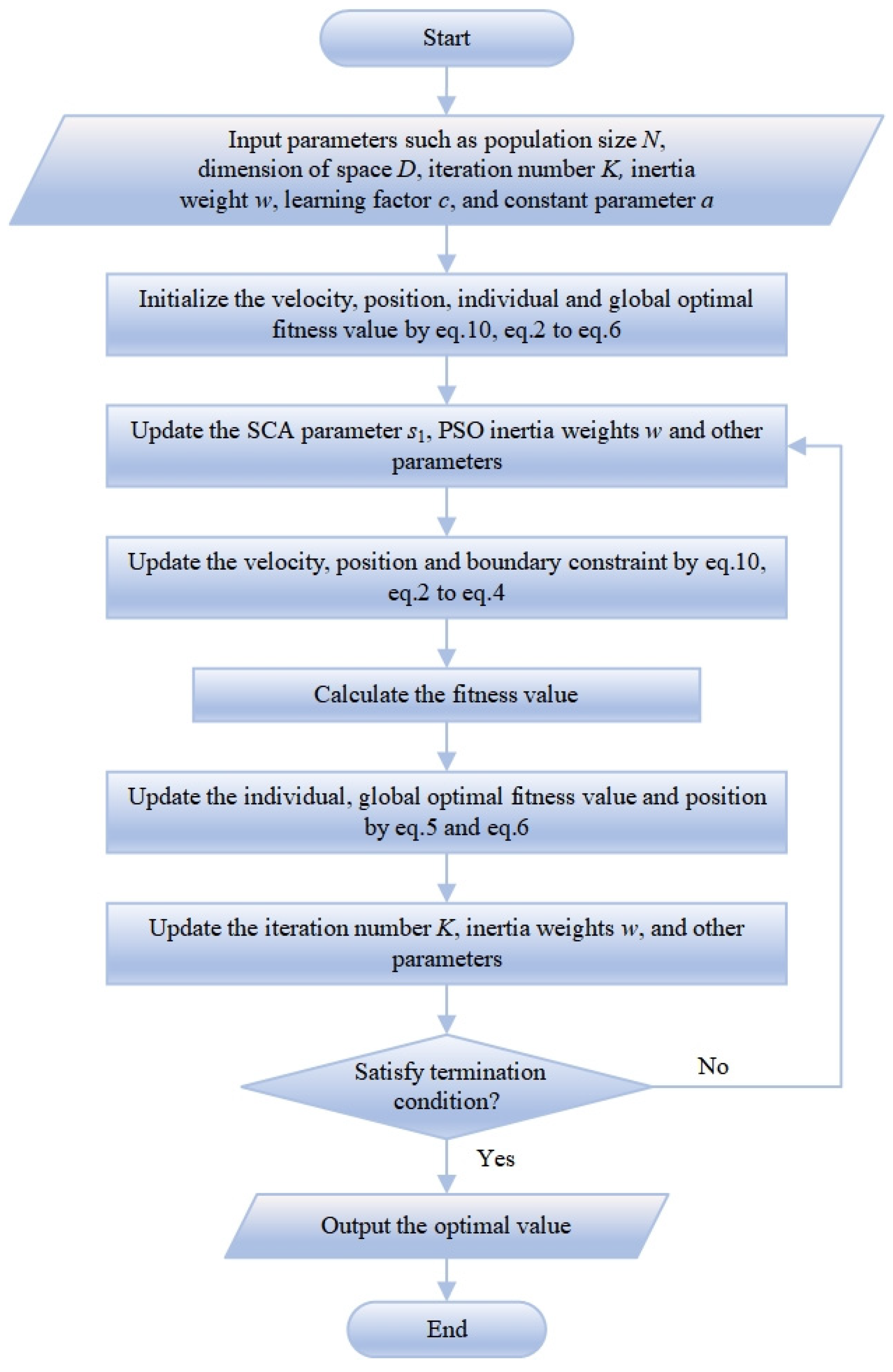
3.2. Proposed Velocity Four Sine Cosine Particle Swarm Optimization (VFSCPSO)
| Algorithm 3 Velocity Four Sine Cosine Particle Swarm Optimization |
| Input: Initialize population N, dimension D, iteration K, learning factors , , , inertia weight w, velocity boundaries , , position boundaries , constant parameter a Output: Optimal fitness value
|
3.3. Complexity Discussion
4. Experiment and Analysis
4.1. Experimental Settings
4.2. Experimental Results and Analysis
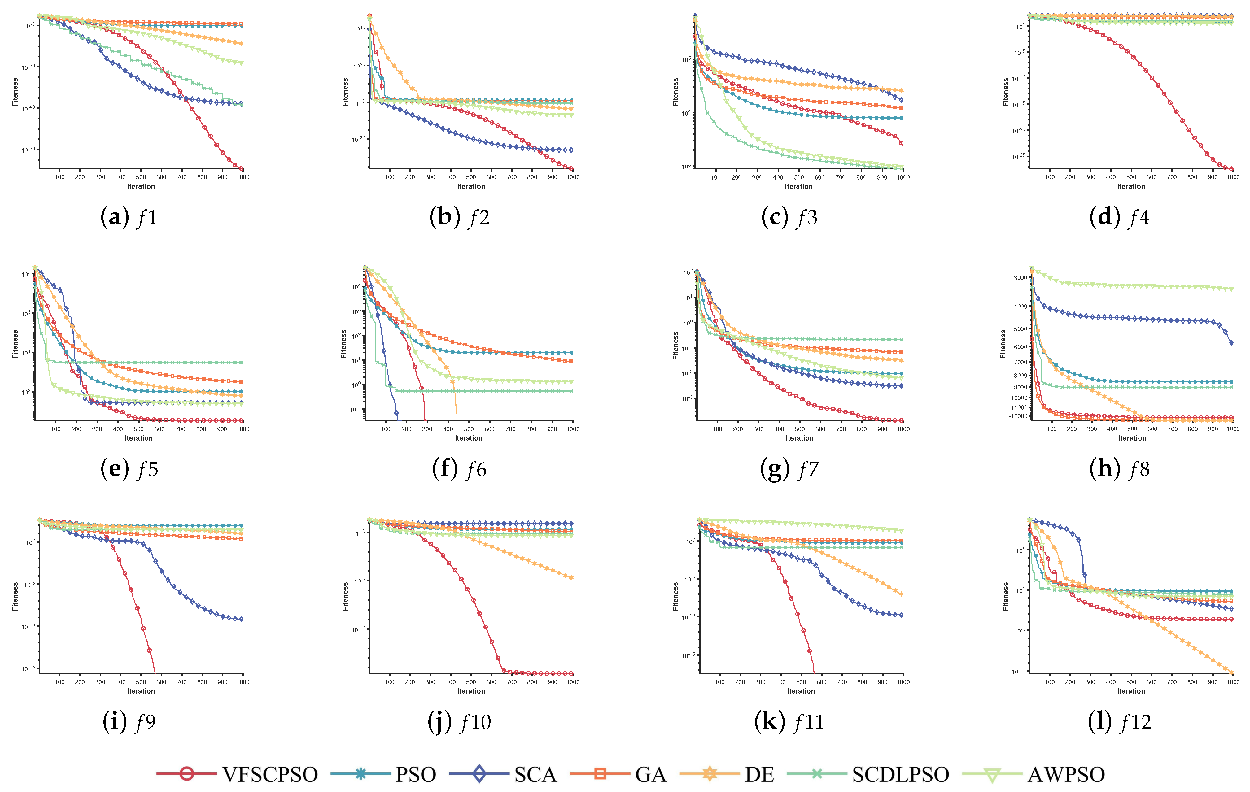
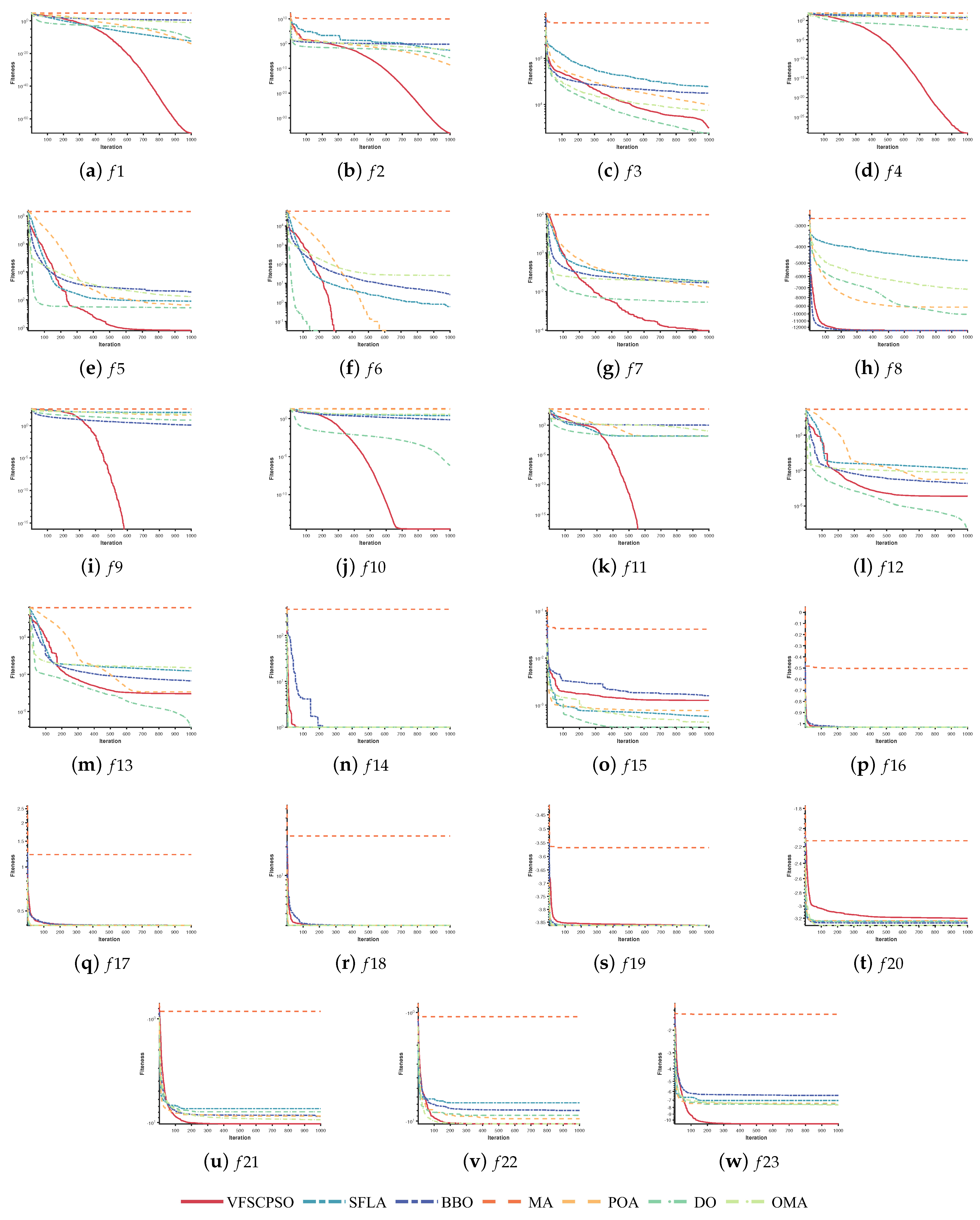
4.2.1. Performance of Algorithm in Standard Environment
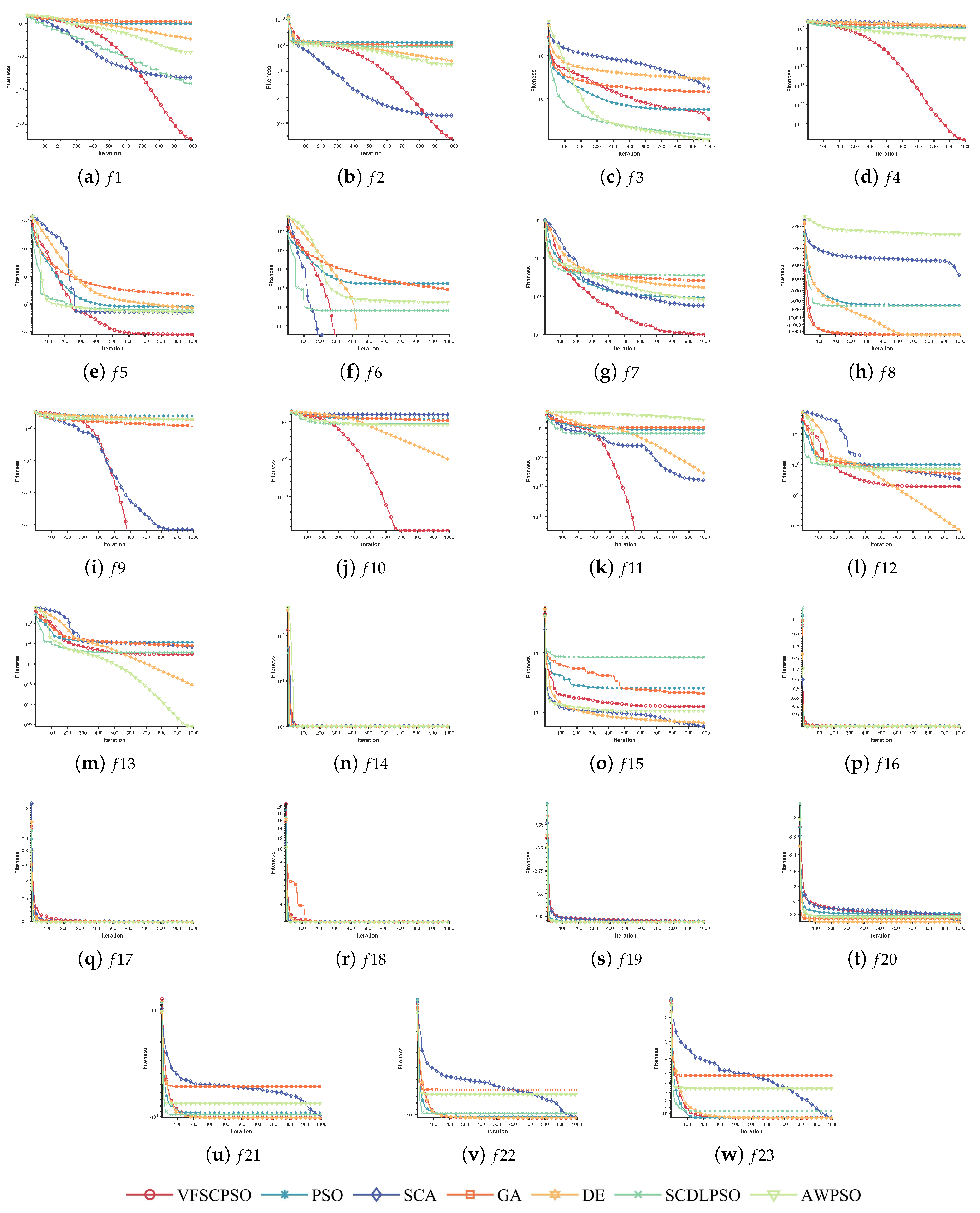
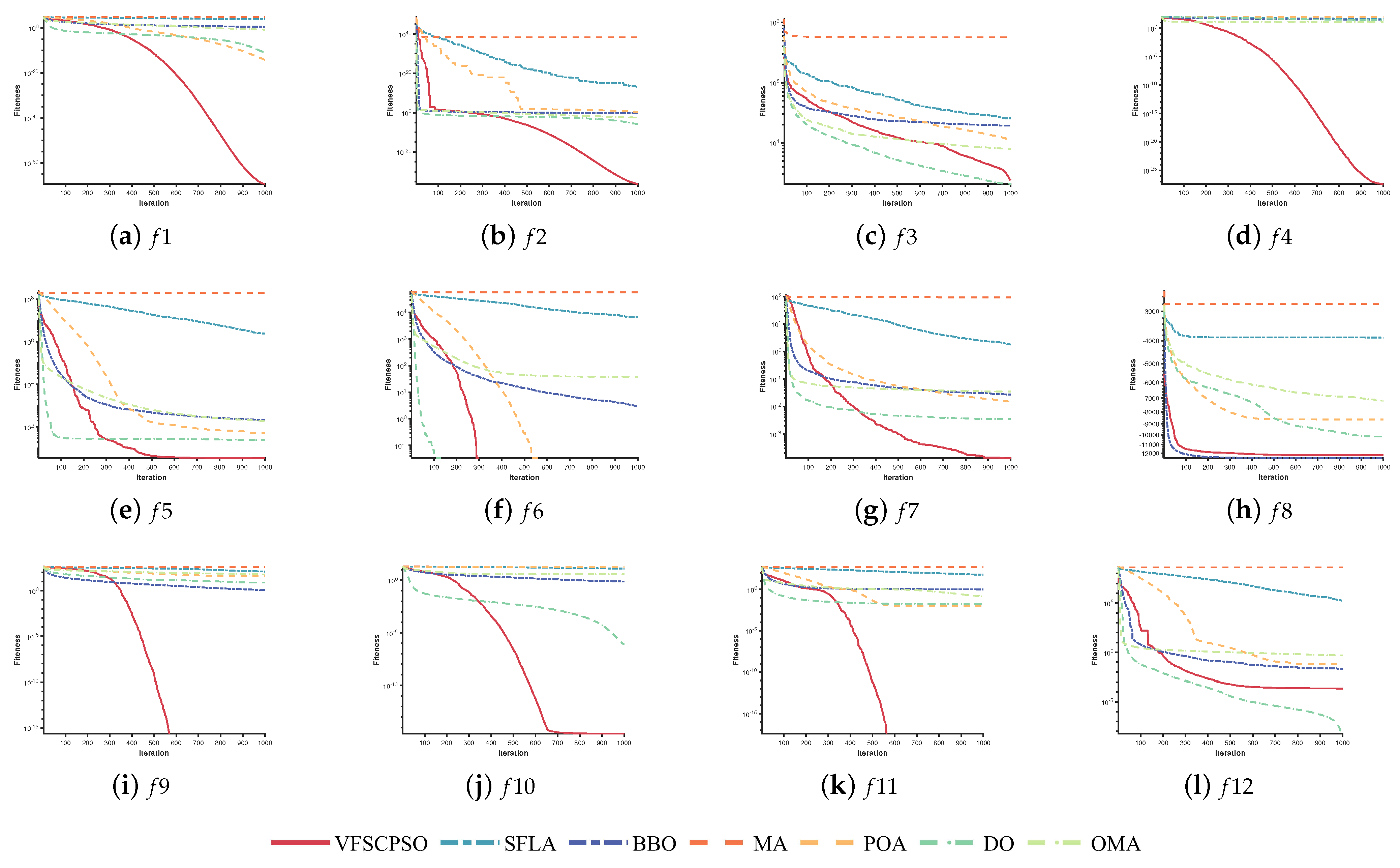
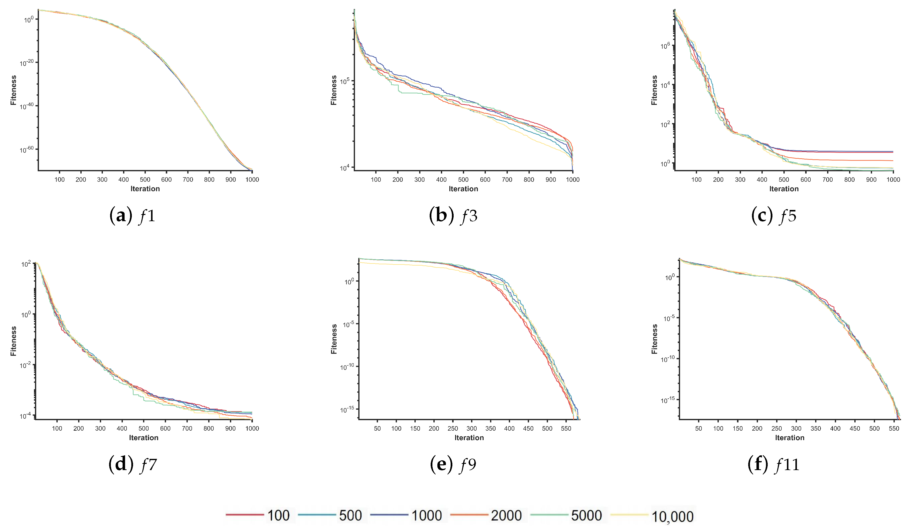
4.2.2. Performance of Algorithms in High-Dimensional Environment
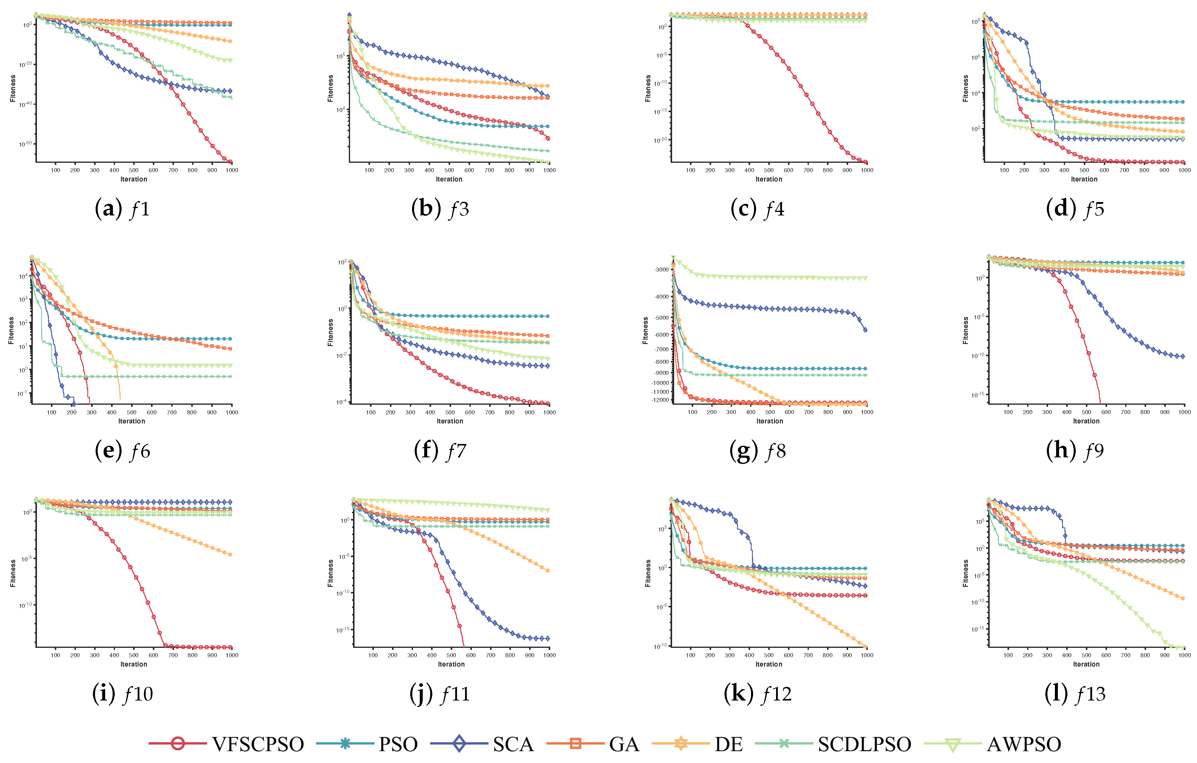
4.2.3. Performance of Algorithms in Large-Scale Environment
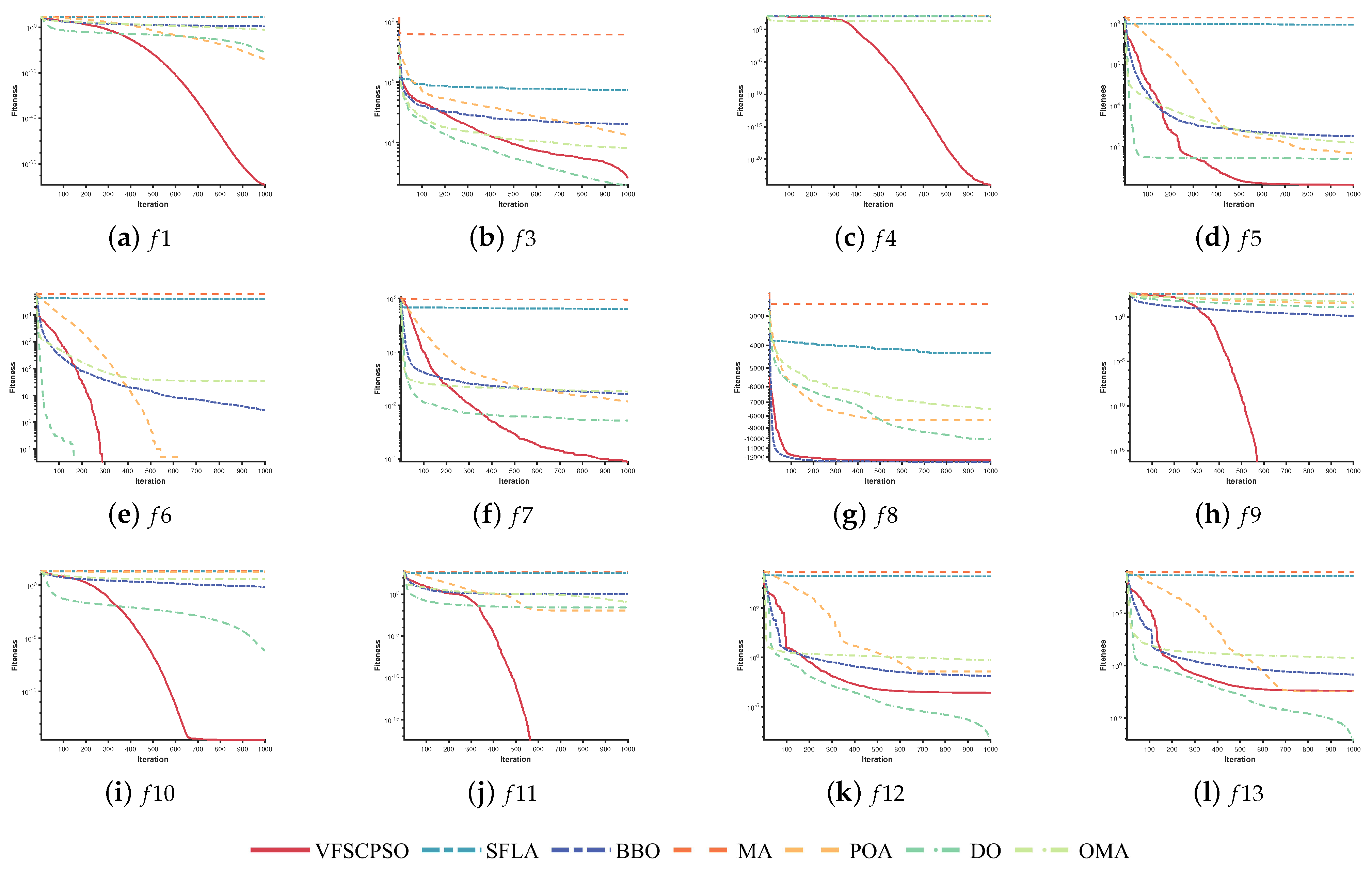
4.2.4. Performance of Algorithm in Ultra-Large-Scale Environment
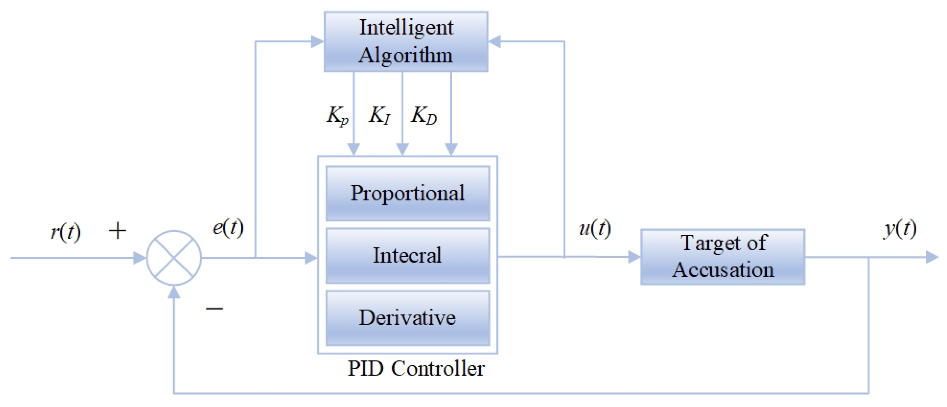
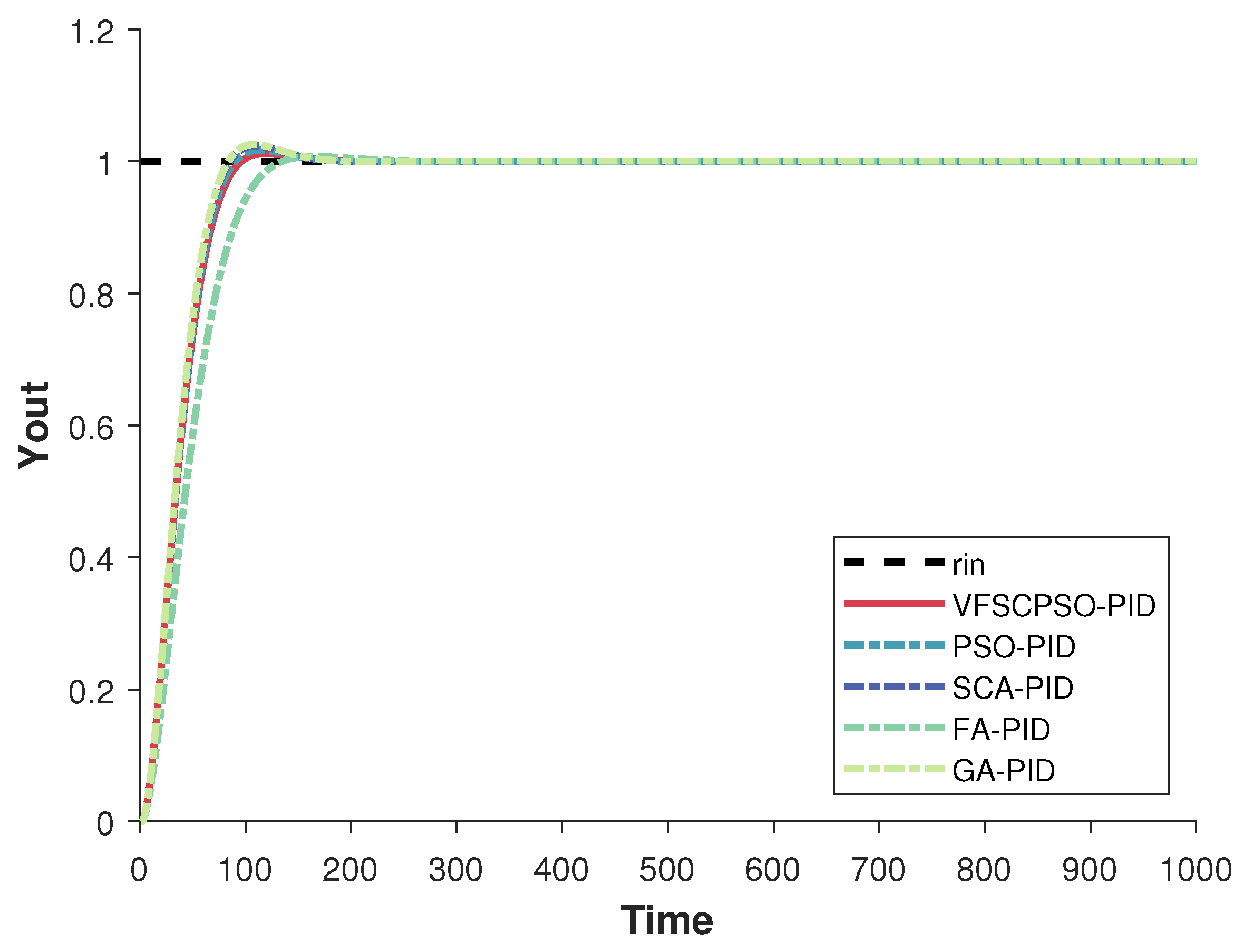
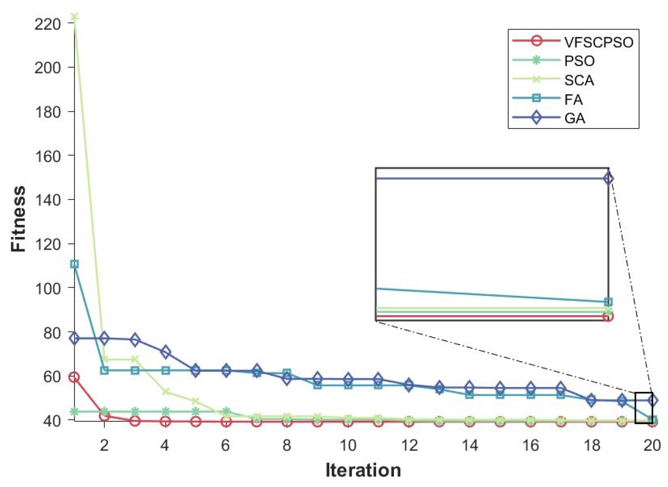
4.2.5. Application in PID Parameter Tuning
- Variables: In optimization problems, variables are quantities that can be adjusted or changed. They represent the decision variables or parameters of the optimal solution sought by the optimization method. In problems in engineering, science, or economics, variables can be various adjustable parameters such as size, velocity, temperature, etc. In the PID parameter-tuning problem, the variables usually are the parameters of the PID controller, i.e., the proportionality coefficients, the integration time, and the differentiation time. The response characteristics of the PID controller are controlled by tuning these parameters.
- Objective function: The objective function is the quantity to be maximized or minimized in an optimization problem. It represents the objective of the optimization. The form of the objective function depends on the specific problem; it can represent cost, benefit, efficiency, distance, or any other metric to be optimized. The objective is to bring these performance metrics to their optimal values or to satisfy certain requirements. In PID parameter-tuning problems, the objective function is usually the performance metric of the control system.
- Constraints: Constraints are conditions or restrictions that must be satisfied so that the solution is considered feasible or acceptable. Constraints define the space of feasible solutions and within this space the optimal solution is sought. Constraints usually come from physical limitations, technical limitations, regulations, or other constraints. In the case of PID parameter-tuning problems, constraints may come from the stability requirements of the control system. There may also be engineering constraints from practical applications, such as the range of PID parameter values or the performance requirements of the control system. The constraints are handled using a penalty function approach in this paper. There may also be engineering constraints from practical applications, such as the range of PID parameter values or the performance requirements of the control system. The constraints are handled using a penalty function approach in the paper. By introducing a penalty function, the constraints are incorporated into the objective function, thus transforming the original problem into an unconstrained optimization problems.
- Optimization method: An optimization method is a technique used to search for optimal solutions that minimize or maximize an objective function. The selection of an appropriate optimization method depends on the nature of the problem, constraints, objective function, and the availability of computational resources. The optimization method described in Section 1 can be used in the PID parameter-tuning problem, and therefore, will not be repeated here.
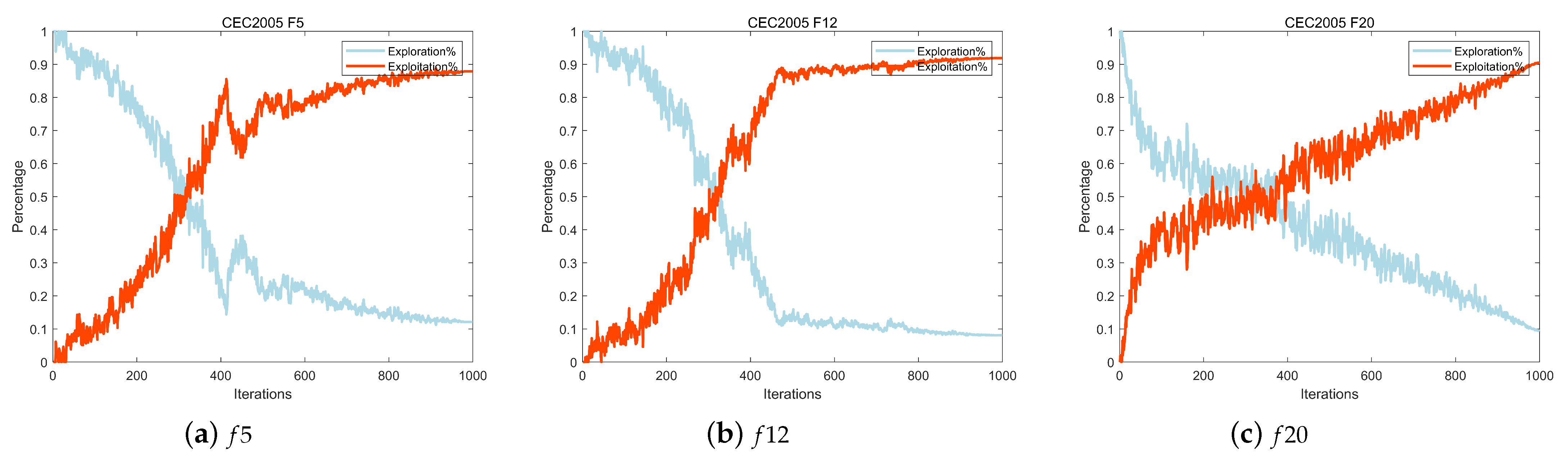
4.2.6. Analysis of VFSCPSO’s Exploration and Exploitation
4.2.7. Analysis of VFSCPSO’s Disadvantages
5. Conclusions
Author Contributions
Funding
Data Availability Statement
Conflicts of Interest
Appendix A. CEC2005 Test Suite of 23 Benchmark Functions
Appendix A.1. Sphere Function
Appendix A.2. Schwefel’s Problem 2.22
Appendix A.3. Schwefel’s Problem 1.2
Appendix A.4. Schwefel’s Problem 2.21
Appendix A.5. Generalized Rosenbrock’s Function
Appendix A.6. Step Function
Appendix A.7. Quartic Function i.e., Noise
Appendix A.8. Generalized Schwefel’s Problem 2.26
Appendix A.9. Generalized Rastrigin’s Function
Appendix A.10. Ackley’s Function
Appendix A.11. Generalized Griewank’s Function
Appendix A.12. Generalized Penalized Function 1
Appendix A.13. Generalized Penalized Function 2
Appendix A.14. Shekel’s Foxholes Function
Appendix A.15. Kowalik’s Function
Appendix A.16. Six-Hump Camel-Back Function
Appendix A.17. Branin Function
Appendix A.18. Goldstein Price Function
Appendix A.19. Hartman’s Family 1
Appendix A.20. Hartman’s Family 2
Appendix A.21. Shekel’s Family 1
Appendix A.22. Shekel’s Family 2
Appendix A.23. Shekel’s Family 3
References
- Holland, J.H. Adaptation in Natural and Artificial Systems: An Introductory Analysis with Applications to Biology; MIT Press: Cambridge, MA, USA, 1975. [Google Scholar]
- Storn, R.; Price, K. Differential evolution—A simple and efficient heuristic for global optimization over continuous spaces. J. Glob. Optim. 1997, 11, 341–359. [Google Scholar] [CrossRef]
- Zhao, S.; Zhang, T.; Ma, S.; Chen, M. Dandelion Optimizer: A nature-inspired metaheuristic algorithm for engineering applications. Eng. Appl. Artif. Intell. 2022, 114, 105075. [Google Scholar] [CrossRef]
- Simon, D. Biogeography-based optimization. IEEE Trans. Evol. Comput. 2008, 12, 702–713. [Google Scholar] [CrossRef]
- Kennedy, J.; Eberhart, R. Particle swarm optimization. In Proceedings of the ICNN’95-International Conference on Neural Networks, Perth, Australia, 27 November–1 December 1995; Volume 4, pp. 1942–1948. [Google Scholar] [CrossRef]
- Eusuff, M.M.; Lansey, K.E. Optimization of water distribution network design using the shuffled frog leaping algorithm. J. Water Resour. Plan. Manag. 2003, 129, 210–225. [Google Scholar] [CrossRef]
- Yang, X.S. Firefly algorithms for multimodal optimization. In Proceedings of the International Symposium on Stochastic Algorithms, Sapporo, Japan, 26–28 October 2009; pp. 169–178. [Google Scholar] [CrossRef]
- Zervoudakis, K.; Tsafarakis, S. A mayfly optimization algorithm. Comput. Ind. Eng. 2020, 145, 106559. [Google Scholar] [CrossRef]
- Wang, J.; Yang, B.; Chen, Y.; Zeng, K.; Zhang, H.; Shu, H.; Chen, Y. Novel phasianidae inspired peafowl (Pavo muticus/cristatus) optimization algorithm: Design, evaluation, and SOFC models parameter estimation. Sustain. Energy Technol. Assess. 2022, 50, 101825. [Google Scholar] [CrossRef]
- Bertsimas, D.; Tsitsiklis, J. Simulated annealing. Stat. Sci. 1993, 8, 10–15. [Google Scholar] [CrossRef]
- Mirjalili, S. SCA: A sine cosine algorithm for solving optimization problems. Knowl.-Based Syst. 2016, 96, 120–133. [Google Scholar] [CrossRef]
- Das, B.; Mukherjee, V.; Das, D. Student psychology based optimization algorithm: A new population based optimization algorithm for solving optimization problems. Adv. Eng. Softw. 2020, 146, 102804. [Google Scholar] [CrossRef]
- Cheng, M.Y.; Sholeh, M.N. Optical microscope algorithm: A new metaheuristic inspired by microscope magnification for solving engineering optimization problems. Knowl.-Based Syst. 2023, 279, 110939. [Google Scholar] [CrossRef]
- Nayak, J.; Swapnarekha, H.; Naik, B.; Dhiman, G.; Vimal, S. 25 Years of Particle Swarm Optimization: Flourishing Voyage of Two Decades. Arch. Comput. Methods Eng. 2023, 30, 1663–1725. [Google Scholar] [CrossRef]
- Yu, Z.; Si, Z.; Li, X.; Wang, D.; Song, H. A novel hybrid particle swarm optimization algorithm for path planning of UAVs. IEEE Internet Things J. 2022, 9, 22547–22558. [Google Scholar] [CrossRef]
- Wang, C.; Wang, Z.; Han, F.; Dong, H.; Liu, H. A novel PID-like particle swarm optimizer: On terminal convergence analysis. Complex Intell. Syst. 2022, 8, 1217–1228. [Google Scholar] [CrossRef]
- Tijjani, S.; Ab Wahab, M.N.; Mohd Noor, M.H. An enhanced particle swarm optimization with position update for optimal feature selection. Expert Syst. Appl. 2024, 247, 123337. [Google Scholar] [CrossRef]
- Suriyan, K.; Nagarajan, R. Particle Swarm Optimization in Biomedical Technologies: Innovations, Challenges, and Opportunities. In Emerging Technologies for Health Literacy and Medical Practice; IGI Global: Hershey, PA, USA, 2024; pp. 220–238. [Google Scholar] [CrossRef]
- Li, F.; Yue, Q.; Liu, Y.; Ouyang, H.; Gu, F. A fast density peak clustering based particle swarm optimizer for dynamic optimization. Expert Syst. Appl. 2024, 236, 121254. [Google Scholar] [CrossRef]
- Shi, Y.; Eberhart, R.C. Empirical study of particle swarm optimization. In Proceedings of the 1999 Congress on Evolutionary Computation-CEC99 (Cat. No. 99TH8406), Washington, DC, USA, 6–9 July 1999; Volume 3, pp. 1945–1950. [Google Scholar] [CrossRef]
- Liu, W.; Wang, Z.; Yuan, Y.; Zeng, N.; Hone, K.; Liu, X. A novel sigmoid-function-based adaptive weighted particle swarm optimizer. IEEE Trans. Cybern. 2019, 51, 1085–1093. [Google Scholar] [CrossRef] [PubMed]
- Refaat, A.; Elbaz, A.; Khalifa, A.E.; Mohamed Elsakka, M.; Kalas, A.; Hegazy Elfar, M. Performance evaluation of a novel self-tuning particle swarm optimization algorithm-based maximum power point tracker for porton exchange membrane fuel cells under different operating conditions. Energy Convers. Manag. 2024, 301, 118014. [Google Scholar] [CrossRef]
- Zhang, J.; Zhang, J.; Ji, W. Particle swarm optimization algorithm with self-correcting and dimension-by-dimension learning capabilities. J. Chin. Comput. Syst. 2021, 42, 919–926. [Google Scholar]
- Xue, Y.; Tang, T.; Pang, W.; Liu, A.X. Self-adaptive parameter and strategy based particle swarm optimization for large-scale feature selection problems with multiple classifiers. Appl. Soft Comput. 2020, 88, 106031. [Google Scholar] [CrossRef]
- Kaseb, Z.; Rahbar, M. Towards CFD-based optimization of urban wind conditions: Comparison of Genetic algorithm, Particle Swarm Optimization, and a hybrid algorithm. Sustain. Cities Soc. 2022, 77, 103565. [Google Scholar] [CrossRef]
- Shams, M.Y.; El-kenawy, E.S.M.; Ibrahim, A.; Elshewey, A.M. A hybrid dipper throated optimization algorithm and particle swarm optimization (DTPSO) model for hepatocellular carcinoma (HCC) prediction. Biomed. Signal Process. Control. 2023, 85, 104908. [Google Scholar] [CrossRef]
- Major Advances in Particle Swarm Optimization: Theory, Analysis, and Application. Swarm Evol. Comput. 2021, 63, 100868. [CrossRef]
- Shami, T.M.; El-Saleh, A.A.; Alswaitti, M.; Al-Tashi, Q.; Summakieh, M.A.; Mirjalili, S. Particle Swarm Optimization: A Comprehensive Survey. IEEE Access 2022, 10, 10031–10061. [Google Scholar] [CrossRef]
- Yang, X.; Wang, R.; Zhao, D.; Yu, F.; Huang, C.; Heidari, A.A.; Cai, Z.; Bourouis, S.; Algarni, A.D.; Chen, H. An adaptive quadratic interpolation and rounding mechanism sine cosine algorithm with application to constrained engineering optimization problems. Expert Syst. Appl. 2023, 213, 119041. [Google Scholar] [CrossRef]
- Gul, H.H.; Egrioglu, E.; Bas, E. Statistical learning algorithms for dendritic neuron model artificial neural network based on sine cosine algorithm. Inf. Sci. 2023, 629, 398–412. [Google Scholar] [CrossRef]
- Akay, R.; Yildirim, M.Y. Multi-strategy and self-adaptive differential sine-cosine algorithm for multi-robot path planning. Expert Syst. Appl. 2023, 232, 120849. [Google Scholar] [CrossRef]
- Rizk-Allah, R.M. An improved sine–cosine algorithm based on orthogonal parallel information for global optimization. Soft Comput. 2019, 23, 7135–7161. [Google Scholar] [CrossRef]
- Zhou, W.; Wang, P.; Heidari, A.A.; Zhao, X.; Chen, H. Spiral Gaussian mutation sine cosine algorithm: Framework and comprehensive performance optimization. Expert Syst. Appl. 2022, 209, 118372. [Google Scholar] [CrossRef]
- Ma, H.; Zhang, C.; Peng, T.; Nazir, M.S.; Li, Y. An integrated framework of gated recurrent unit based on improved sine cosine algorithm for photovoltaic power forecasting. Energy 2022, 256, 124650. [Google Scholar] [CrossRef]
- Hamad, Q.S.; Samma, H.; Suandi, S.A.; Mohamad-Saleh, J. Q-learning embedded sine cosine algorithm (QLESCA). Expert Syst. Appl. 2022, 193, 116417. [Google Scholar] [CrossRef]
- Cheng, R.; Jin, Y. A social learning particle swarm optimization algorithm for scalable optimization. Inf. Sci. 2015, 291, 43–60. [Google Scholar] [CrossRef]
- Chakraborty, S.; Saha, A.K.; Chakraborty, R.; Saha, M. An enhanced whale optimization algorithm for large scale optimization problems. Knowl.-Based Syst. 2021, 233, 107543. [Google Scholar] [CrossRef]
- Xu, H.Q.; Gu, S.; Fan, Y.C.; Li, X.S.; Zhao, Y.F.; Zhao, J.; Wang, J.J. A strategy learning framework for particle swarm optimization algorithm. Inf. Sci. 2023, 619, 126–152. [Google Scholar] [CrossRef]
- Wang, F.; Wang, X.; Sun, S. A reinforcement learning level-based particle swarm optimization algorithm for large-scale optimization. Inf. Sci. 2022, 602, 298–312. [Google Scholar] [CrossRef]
- Yi, J.H.; Xing, L.N.; Wang, G.G.; Dong, J.; Vasilakos, A.V.; Alavi, A.H.; Wang, L. Behavior of crossover operators in NSGA-III for large-scale optimization problems. Inf. Sci. 2020, 509, 470–487. [Google Scholar] [CrossRef]
- Ziegler, J.G.; Nichols, N.B. Optimum settings for automatic controllers. Trans. Am. Soc. Mech. Eng. 1942, 64, 759–765. [Google Scholar] [CrossRef]
- Cao, F. PID controller optimized by genetic algorithm for direct-drive servo system. Neural Comput. Appl. 2020, 32, 23–30. [Google Scholar] [CrossRef]
- Zhu, Y.; Jiao, J. Automatic Control System Design for Industrial Robots Based on Simulated Annealing and PID Algorithms. Adv. Multimed. 2022, 2022, 9226576. [Google Scholar] [CrossRef]
- Huang, M.; Tian, M.; Liu, Y.; Zhang, Y.; Zhou, J. Parameter optimization of PID controller for water and fertilizer control system based on partial attraction adaptive firefly algorithm. Sci. Rep. 2022, 12, 12182. [Google Scholar] [CrossRef] [PubMed]
- Shi, Y.; Eberhart, R.C. Parameter selection in particle swarm optimization. In Proceedings of the Evolutionary Programming VII: 7th International Conference, EP98, San Diego, CA, USA, 25–27 March 1998; pp. 591–600. [Google Scholar] [CrossRef]
- Suganthan, P.N.; Hansen, N.; Liang, J.J.; Deb, K.; Chen, Y.P.; Auger, A.; Tiwari, S. Problem definitions and evaluation criteria for the CEC 2005 special session on real-parameter optimization. Kangal Rep. 2005, 2005005, 2005. [Google Scholar]
- Derrac, J.; García, S.; Molina, D.; Herrera, F. A practical tutorial on the use of nonparametric statistical tests as a methodology for comparing evolutionary and swarm intelligence algorithms. Swarm Evol. Comput. 2011, 1, 3–18. [Google Scholar] [CrossRef]
- Hussain, K.; Salleh, M.N.M.; Cheng, S.; Shi, Y. On the exploration and exploitation in popular swarm-based metaheuristic algorithms. Neural Comput. Appl. 2019, 31, 7665–7683. [Google Scholar] [CrossRef]


| Problem | Name | Dimensions | Search Space | |
|---|---|---|---|---|
| Sphere Function | 30 | 0 | ||
| Schwefel’s Problem 2.22 | 30 | 0 | ||
| Schwefel’s Problem 1.2 | 30 | 0 | ||
| Schwefel’s Problem 2.21 | 30 | 0 | ||
| Generalized Rosenbrock’s Function | 30 | 0 | ||
| Step Function | 30 | 0 | ||
| Quartic Function, i.e., Noise | 30 | 0 | ||
| Generalized Schwefel’s Problem 2.26 | 30 | −12,569.5 | ||
| Generalized Rastrigin’s Function | 30 | 0 | ||
| Ackley’s Function | 30 | 0 | ||
| Generalized Griewank’s Function | 30 | 0 | ||
| Generalized Penalized Function 1 | 30 | 0 | ||
| Generalized Penalized Function 2 | 30 | 0 | ||
| Shekel’s Foxholes Function | 2 | 0.998003838 | ||
| Kowalik’s Function | 4 | 0.0003075 | ||
| Six-Hump Camel-Back Function | 2 | −1.03162845 | ||
| Branin Function | 2 | 0.397887358 | ||
| Goldstein Price Function | 2 | 3 | ||
| Hartman’s Family 1 | 3 | −3.86278215 | ||
| Hartman’s Family 2 | 6 | −3.32199517 | ||
| Shekel’s Family 1 | 4 | −10.1531997 | ||
| Shekel’s Family 2 | 4 | −10.4029406 | ||
| Shekel’s Family 3 | 4 | −10.5364 |
| Problem | Metric | GA | DE | PSO | SCA | AWPSO | SCDLPSO | VFSCPSO |
|---|---|---|---|---|---|---|---|---|
| best | 3.24E+00 | 1.82E−10 | 4.15E−02 | 1.37E−48 | 6.77E−23 | 4.40E−46 | 3.63E−74 | |
| mean | 6.63E+00 | 3.23E−10 | 6.12E−01 | 6.32E−33 | 9.66E−18 | 1.59E−38 | 1.69E−69 | |
| worst | 1.19E+01 | 4.69E−10 | 2.00E+00 | 1.88E−31 | 2.65E−16 | 4.57E−37 | 4.54E−68 | |
| std | 2.27E+00 | 7.16E−11 | 4.67E−01 | 3.43E−32 | 4.83E−17 | 8.35E−38 | 8.27E−69 | |
| best | 6.38E−01 | 5.19E−07 | 9.08E−01 | 1.32E−32 | 1.47E−11 | 3.33E−21 | 6.24E−39 | |
| mean | 8.37E−01 | 9.29E−07 | 1.08E+01 | 9.33E−28 | 5.28E−08 | 3.33E−01 | 7.44E−37 | |
| worst | 1.04E+00 | 1.28E−06 | 3.12E+01 | 1.85E−26 | 5.11E−07 | 1.00E+01 | 6.17E−36 | |
| std | 1.20E−01 | 1.79E−07 | 8.84E+00 | 3.38E−27 | 1.25E−07 | 1.83E+00 | 1.25E−36 | |
| best | 6.62E+03 | 1.63E+04 | 1.44E+03 | 8.50E+03 | 3.76E+02 | 8.09E+01 | 8.66E−02 | |
| mean | 1.38E+04 | 2.87E+04 | 5.54E+03 | 1.72E+04 | 1.09E+03 | 1.43E+03 | 3.06E+03 | |
| worst | 3.31E+04 | 3.93E+04 | 3.66E+04 | 2.46E+04 | 2.71E+03 | 6.31E+03 | 5.24E+04 | |
| std | 5.82E+03 | 6.31E+03 | 6.92E+03 | 4.04E+03 | 5.10E+02 | 1.81E+03 | 1.38E+04 | |
| best | 3.31E+00 | 3.89E+00 | 8.15E−01 | 6.70E−11 | 4.68E−04 | 5.69E−01 | 1.89E−32 | |
| mean | 4.98E+00 | 4.86E+00 | 1.93E+00 | 2.97E+00 | 2.10E−03 | 1.42E+00 | 6.45E−30 | |
| worst | 6.55E+00 | 5.76E+00 | 3.24E+00 | 1.95E+01 | 6.04E−03 | 3.67E+00 | 6.49E−29 | |
| std | 6.92E−01 | 4.81E−01 | 7.09E−01 | 5.52E+00 | 1.33E−03 | 6.40E−01 | 1.42E−29 | |
| best | 1.61E+02 | 3.68E+01 | 3.01E+01 | 2.60E+01 | 7.40E+00 | 9.90E−04 | 6.34E−02 | |
| mean | 4.39E+02 | 5.31E+01 | 6.94E+01 | 2.65E+01 | 2.84E+01 | 3.56E+01 | 6.15E−01 | |
| worst | 2.35E+03 | 8.46E+01 | 2.97E+02 | 2.69E+01 | 7.86E+01 | 8.14E+01 | 4.07E+00 | |
| std | 4.35E+02 | 1.31E+01 | 5.97E+01 | 2.28E−01 | 1.67E+01 | 2.84E+01 | 8.61E−01 | |
| best | 1.00E+00 | 0.00E+00 | 1.00E+00 | 0.00E+00 | 0.00E+00 | 0.00E+00 | 0.00E+00 | |
| mean | 7.97E+00 | 0.00E+00 | 1.71E+01 | 0.00E+00 | 1.77E+00 | 6.33E−01 | 0.00E+00 | |
| worst | 1.60E+01 | 0.00E+00 | 3.40E+01 | 0.00E+00 | 1.00E+01 | 7.00E+00 | 0.00E+00 | |
| std | 3.22E+00 | 0.00E+00 | 6.96E+00 | 0.00E+00 | 2.60E+00 | 1.56E+00 | 0.00E+00 | |
| best | 2.00E−02 | 1.68E−02 | 2.27E−03 | 3.46E−04 | 3.09E−03 | 9.75E−03 | 1.45E−05 | |
| mean | 6.53E−02 | 2.85E−02 | 8.35E−03 | 3.24E−03 | 6.40E−03 | 1.25E−01 | 9.41E−05 | |
| worst | 1.34E−01 | 4.34E−02 | 1.79E−02 | 1.37E−02 | 1.44E−02 | 2.70E+00 | 5.07E−04 | |
| std | 2.67E−02 | 6.71E−03 | 4.77E−03 | 2.78E−03 | 2.71E−03 | 4.88E−01 | 1.08E−04 | |
| best | −1.26E+04 | −1.26E+04 | −1.00E+04 | −6.93E+03 | −4.11E+03 | −1.06E+04 | −1.26E+04 | |
| mean | −1.26E+04 | −1.26E+04 | −8.49E+03 | −5.76E+03 | −3.33E+03 | −8.58E+03 | −1.25E+04 | |
| worst | −1.25E+04 | −1.26E+04 | −5.17E+03 | −5.26E+03 | −2.79E+03 | −7.28E+03 | −1.22E+04 | |
| std | 5.39E+00 | 3.82E−05 | 1.01E+03 | 3.19E+02 | 3.41E+02 | 8.80E+02 | 7.89E+01 | |
| best | 1.38E+00 | 1.84E+01 | 3.25E+01 | 0.00E+00 | 1.69E+01 | 1.09E+01 | 0.00E+00 | |
| mean | 2.63E+00 | 2.39E+01 | 9.38E+01 | 1.78E−16 | 3.13E+01 | 3.15E+01 | 0.00E+00 | |
| worst | 4.13E+00 | 3.00E+01 | 1.54E+02 | 5.33E−15 | 5.87E+01 | 7.16E+01 | 0.00E+00 | |
| std | 7.44E−01 | 2.63E+00 | 3.41E+01 | 9.73E−16 | 9.35E+00 | 1.71E+01 | 0.00E+00 | |
| best | 9.94E−01 | 5.95E−06 | 4.47E−01 | 4.44E−15 | 1.74E−12 | 3.24E−14 | 8.88E−16 | |
| mean | 1.39E+00 | 9.18E−06 | 2.34E+00 | 8.80E+00 | 3.87E−01 | 5.19E−01 | 3.14E−15 | |
| worst | 1.87E+00 | 2.25E−05 | 3.94E+00 | 2.01E+01 | 2.32E+00 | 1.90E+00 | 4.44E−15 | |
| std | 2.13E−01 | 3.12E−06 | 9.03E−01 | 1.00E+01 | 7.97E−01 | 6.90E−01 | 1.74E−15 | |
| best | 1.02E+00 | 1.78E−09 | 2.26E−01 | 0.00E+00 | 1.51E+01 | 7.40E−03 | 0.00E+00 | |
| mean | 1.06E+00 | 1.61E−08 | 5.83E−01 | 1.29E−09 | 2.20E+01 | 1.20E−01 | 0.00E+00 | |
| worst | 1.10E+00 | 1.02E−07 | 9.60E−01 | 3.87E−08 | 2.57E+01 | 4.07E−01 | 0.00E+00 | |
| std | 1.98E−02 | 2.44E−08 | 2.13E−01 | 7.06E−09 | 2.48E+00 | 9.44E−02 | 0.00E+00 | |
| best | 7.48E−03 | 7.22E−12 | 5.97E−02 | 2.20E−03 | 2.04E−24 | 8.40E−23 | 8.56E−06 | |
| mean | 2.80E−02 | 1.34E−11 | 9.14E−01 | 4.18E−03 | 1.38E−01 | 2.02E−01 | 2.21E−04 | |
| worst | 8.77E−02 | 2.88E−11 | 4.15E+00 | 7.35E−03 | 8.30E−01 | 2.98E+00 | 5.71E−04 | |
| std | 1.81E−02 | 4.71E−12 | 9.53E−01 | 1.50E−03 | 2.18E−01 | 5.59E−01 | 1.42E−04 | |
| best | 1.38E−01 | 2.11E−11 | 8.58E−01 | 3.34E−02 | 1.82E−25 | 1.35E−32 | 2.89E−04 | |
| mean | 3.84E−01 | 4.44E−11 | 2.57E+00 | 1.91E−01 | 3.20E−21 | 6.95E−03 | 2.49E−03 | |
| worst | 7.05E−01 | 8.25E−11 | 5.09E+00 | 4.91E−01 | 3.83E−20 | 5.48E−02 | 7.32E−03 | |
| std | 1.47E−01 | 1.48E−11 | 1.32E+00 | 1.24E−01 | 8.89E−21 | 1.27E−02 | 1.90E−03 | |
| best | 9.98E−01 | 9.98E−01 | 9.98E−01 | 9.98E−01 | 9.98E−01 | 9.98E−01 | 9.98E−01 | |
| mean | 9.98E−01 | 9.98E−01 | 9.98E−01 | 9.98E−01 | 9.98E−01 | 9.98E−01 | 9.98E−01 | |
| worst | 9.98E−01 | 9.98E−01 | 9.98E−01 | 9.98E−01 | 9.98E−01 | 9.98E−01 | 9.98E−01 | |
| std | 2.23E−10 | 3.39E−16 | 3.39E−16 | 5.14E−12 | 3.39E−16 | 3.34E−16 | 1.08E−13 | |
| best | 6.01E−04 | 5.02E−04 | 3.07E−04 | 3.24E−04 | 3.07E−04 | 3.07E−04 | 3.07E−04 | |
| mean | 2.06E−03 | 6.70E−04 | 2.55E−03 | 5.82E−04 | 1.05E−03 | 8.44E−03 | 1.26E−03 | |
| worst | 2.04E−02 | 7.78E−04 | 2.04E−02 | 1.22E−03 | 2.04E−02 | 2.04E−02 | 2.25E−03 | |
| std | 3.52E−03 | 8.38E−05 | 5.05E−03 | 1.94E−04 | 3.66E−03 | 9.91E−03 | 8.35E−04 |
| Problem | Metric | GA | DE | PSO | SCA | AWPSO | SCDLPSO | VFSCPSO |
|---|---|---|---|---|---|---|---|---|
| best | −1.03E+00 | −1.03E+00 | −1.03E+00 | −1.03E+00 | −1.03E+00 | −1.03E+00 | −1.03E+00 | |
| mean | −1.03E+00 | −1.03E+00 | −1.03E+00 | −1.03E+00 | −1.03E+00 | −1.03E+00 | −1.03E+00 | |
| worst | −1.03E+00 | −1.03E+00 | −1.03E+00 | −1.03E+00 | −1.03E+00 | −1.03E+00 | −1.03E+00 | |
| std | 7.62E−06 | 6.78E−16 | 6.78E−16 | 9.74E−09 | 6.78E−16 | 6.78E−16 | 1.83E−09 | |
| best | 3.98E−01 | 3.98E−01 | 3.98E−01 | 3.98E−01 | 3.98E−01 | 3.98E−01 | 3.98E−01 | |
| mean | 3.98E−01 | 3.98E−01 | 3.98E−01 | 3.98E−01 | 3.98E−01 | 3.98E−01 | 3.98E−01 | |
| worst | 3.98E−01 | 3.98E−01 | 3.98E−01 | 3.98E−01 | 3.98E−01 | 3.98E−01 | 3.98E−01 | |
| std | 4.11E−05 | 0.00E+00 | 0.00E+00 | 1.36E−06 | 0.00E+00 | 0.00E+00 | 1.09E−07 | |
| best | 3.00E+00 | 3.00E+00 | 3.00E+00 | 3.00E+00 | 3.00E+00 | 3.00E+00 | 3.00E+00 | |
| mean | 3.00E+00 | 3.00E+00 | 3.00E+00 | 3.00E+00 | 3.00E+00 | 3.00E+00 | 3.00E+00 | |
| worst | 3.00E+00 | 3.00E+00 | 3.00E+00 | 3.00E+00 | 3.00E+00 | 3.00E+00 | 3.00E+00 | |
| std | 5.31E−05 | 1.73E−15 | 1.32E−15 | 2.32E−07 | 9.69E−16 | 1.32E−15 | 1.78E−07 | |
| best | −3.86E+00 | −3.86E+00 | −3.86E+00 | −3.86E+00 | −3.86E+00 | −3.86E+00 | −3.86E+00 | |
| mean | −3.86E+00 | −3.86E+00 | −3.86E+00 | −3.86E+00 | −3.86E+00 | −3.86E+00 | −3.86E+00 | |
| worst | −3.86E+00 | −3.86E+00 | −3.85E+00 | −3.86E+00 | −3.86E+00 | −3.86E+00 | −3.85E+00 | |
| std | 1.07E−06 | 2.71E−15 | 2.73E−03 | 7.53E−05 | 2.71E−15 | 2.71E−15 | 1.45E−03 | |
| best | −3.32E+00 | −3.32E+00 | −3.32E+00 | −3.32E+00 | −3.32E+00 | −3.32E+00 | −3.32E+00 | |
| mean | −3.27E+00 | −3.32E+00 | −3.18E+00 | −3.30E+00 | −3.25E+00 | −3.22E+00 | −3.20E+00 | |
| worst | −3.20E+00 | −3.32E+00 | −2.95E+00 | −3.20E+00 | −3.14E+00 | −3.13E+00 | −3.02E+00 | |
| std | 6.03E−02 | 1.36E−15 | 7.85E−02 | 4.60E−02 | 6.37E−02 | 5.14E−02 | 9.50E−02 | |
| best | −1.03E+01 | −1.03E+01 | −1.03E+01 | −1.03E+01 | −1.03E+01 | −1.03E+01 | −1.03E+01 | |
| mean | −5.25E+00 | −1.03E+01 | −9.29E+00 | −9.94E+00 | −7.58E+00 | −9.63E+00 | −1.03E+01 | |
| worst | −2.66E+00 | −1.03E+01 | −5.10E+00 | −5.10E+00 | −2.66E+00 | −5.09E+00 | −1.03E+01 | |
| std | 3.46E+00 | 3.39E−06 | 2.13E+00 | 1.32E+00 | 3.30E+00 | 1.81E+00 | 5.81E−05 | |
| best | −1.06E+01 | −1.06E+01 | −1.06E+01 | −1.06E+01 | −1.06E+01 | −1.06E+01 | −1.06E+01 | |
| mean | −6.19E+00 | −1.06E+01 | −1.04E+01 | −1.06E+01 | −6.74E+00 | −9.74E+00 | −1.06E+01 | |
| worst | −2.24E+00 | −1.06E+01 | −5.34E+00 | −1.04E+01 | −2.91E+00 | −5.34E+00 | −1.06E+01 | |
| std | 3.55E+00 | 4.51E−05 | 9.65E−01 | 3.58E−02 | 3.50E+00 | 2.00E+00 | 5.62E−05 | |
| best | −1.07E+01 | −1.07E+01 | −1.07E+01 | −1.07E+01 | −1.07E+01 | −1.07E+01 | −1.07E+01 | |
| mean | −5.28E+00 | −1.07E+01 | −1.07E+01 | −1.07E+01 | −6.57E+00 | −9.58E+00 | −1.07E+01 | |
| worst | −2.28E+00 | −1.07E+01 | −1.07E+01 | −1.07E+01 | −3.02E+00 | −5.19E+00 | −1.07E+01 | |
| std | 2.34E+00 | 1.44E−03 | 4.21E−04 | 1.68E−02 | 2.16E+00 | 1.97E+00 | 1.65E−15 | |
| Count | 0 | 9 | 4 | 2 | 6 | 4 | 11 | |
| Avg. rank | 5.695652174 | 2.652173913 | 4.782608696 | 3.782608696 | 3.565217391 | 3.782608696 | 2.608695652 | |
| Overall rank | 7 | 2 | 6 | 4 | 3 | 4 | 1 |
| Problem | Metric | SFLA | BBO | MA | POA | DO | OMA | VFSCPSO |
|---|---|---|---|---|---|---|---|---|
| best | 2.38E−14 | 9.56E−01 | 4.22E+04 | 4.58E−16 | 2.28E−12 | 2.35E−02 | 3.63E−74 | |
| mean | 3.79E−13 | 2.84E+00 | 5.93E+04 | 9.08E−15 | 1.23E−11 | 7.37E−02 | 1.69E−69 | |
| worst | 3.33E−12 | 6.33E+00 | 7.05E+04 | 5.39E−14 | 4.81E−11 | 2.56E−01 | 4.54E−68 | |
| std | 5.97E−13 | 1.35E+00 | 6.16E+03 | 1.17E−14 | 9.27E−12 | 4.95E−02 | 8.27E−69 | |
| best | 1.75E−07 | 3.81E−01 | 2.16E+02 | 3.05E−10 | 8.65E−07 | 2.13E−03 | 6.24E−39 | |
| mean | 1.82E−03 | 5.41E−01 | 9.61E+09 | 2.41E−09 | 2.01E−06 | 4.31E−03 | 7.44E−37 | |
| worst | 5.09E−02 | 7.88E−01 | 1.33E+11 | 1.00E−08 | 6.50E−06 | 2.44E−02 | 6.17E−36 | |
| std | 9.28E−03 | 9.60E−02 | 2.91E+10 | 2.07E−09 | 1.05E−06 | 4.19E−03 | 1.25E−36 | |
| best | 8.30E+03 | 8.47E+03 | 9.27E+04 | 4.06E+03 | 4.89E+02 | 3.93E+03 | 8.66E−02 | |
| mean | 2.43E+04 | 1.76E+04 | 5.91E+05 | 9.68E+03 | 2.38E+03 | 7.39E+03 | 3.06E+03 | |
| worst | 4.89E+04 | 3.88E+04 | 1.74E+06 | 1.54E+04 | 4.66E+03 | 1.35E+04 | 5.24E+04 | |
| std | 1.01E+04 | 6.87E+03 | 3.48E+05 | 3.12E+03 | 1.10E+03 | 2.63E+03 | 1.38E+04 | |
| best | 5.88E−01 | 4.44E+00 | 5.40E+01 | 1.28E−01 | 1.45E−03 | 7.37E+00 | 1.89E−32 | |
| mean | 5.47E+00 | 5.61E+00 | 7.83E+01 | 1.47E+00 | 4.25E−03 | 1.02E+01 | 6.45E−30 | |
| worst | 1.20E+01 | 7.64E+00 | 9.06E+01 | 5.90E+00 | 1.08E−02 | 1.36E+01 | 6.49E−29 | |
| std | 3.08E+00 | 8.21E−01 | 8.13E+00 | 1.40E+00 | 2.08E−03 | 1.37E+00 | 1.42E−29 | |
| best | 1.07E+01 | 1.09E+02 | 1.27E+08 | 1.70E+01 | 2.40E+01 | 8.61E+01 | 6.34E−02 | |
| mean | 7.93E+01 | 3.60E+02 | 2.12E+08 | 4.22E+01 | 2.65E+01 | 1.67E+02 | 6.15E−01 | |
| worst | 3.03E+02 | 3.07E+03 | 2.72E+08 | 1.59E+02 | 9.04E+01 | 2.78E+02 | 4.07E+00 | |
| std | 7.24E+01 | 5.41E+02 | 3.58E+07 | 3.32E+01 | 1.21E+01 | 5.68E+01 | 8.61E−01 | |
| best | 0.00E+00 | 1.00E+00 | 4.45E+04 | 0.00E+00 | 0.00E+00 | 4.00E+00 | 0.00E+00 | |
| mean | 6.00E−01 | 2.57E+00 | 5.89E+04 | 0.00E+00 | 0.00E+00 | 2.59E+01 | 0.00E+00 | |
| worst | 3.00E+00 | 7.00E+00 | 7.23E+04 | 0.00E+00 | 0.00E+00 | 1.26E+02 | 0.00E+00 | |
| std | 8.14E−01 | 1.50E+00 | 5.87E+03 | 0.00E+00 | 0.00E+00 | 2.28E+01 | 0.00E+00 | |
| best | 1.47E−02 | 8.58E−03 | 3.55E+01 | 7.55E−03 | 6.16E−04 | 1.39E−02 | 1.45E−05 | |
| mean | 3.33E−02 | 2.79E−02 | 9.33E+01 | 1.69E−02 | 2.82E−03 | 3.26E−02 | 9.41E−05 | |
| worst | 4.84E−02 | 5.41E−02 | 1.37E+02 | 2.97E−02 | 5.52E−03 | 6.42E−02 | 5.07E−04 | |
| std | 9.29E−03 | 9.86E−03 | 2.48E+01 | 6.16E−03 | 1.13E−03 | 1.22E−02 | 1.08E−04 | |
| best | −6.50E+03 | −1.26E+04 | −3.43E+03 | −1.11E+04 | −1.10E+04 | −8.99E+03 | −1.26E+04 | |
| mean | −4.84E+03 | −1.26E+04 | −2.72E+03 | −9.12E+03 | −1.00E+04 | −7.16E+03 | −1.25E+04 | |
| worst | −3.59E+03 | −1.26E+04 | −2.05E+03 | −7.09E+03 | −9.08E+03 | −5.48E+03 | −1.22E+04 | |
| std | 8.04E+02 | 2.77E+00 | 3.48E+02 | 1.10E+03 | 4.17E+02 | 9.65E+02 | 7.89E+01 | |
| best | 7.07E+01 | 5.75E−01 | 3.34E+02 | 1.89E+01 | 6.72E−12 | 2.39E+01 | 0.00E+00 | |
| mean | 1.11E+02 | 1.23E+00 | 3.80E+02 | 4.40E+01 | 7.27E+00 | 5.45E+01 | 0.00E+00 | |
| worst | 2.05E+02 | 2.68E+00 | 4.34E+02 | 8.36E+01 | 1.70E+01 | 1.00E+02 | 0.00E+00 | |
| std | 3.18E+01 | 4.58E−01 | 3.06E+01 | 1.38E+01 | 5.52E+00 | 2.29E+01 | 0.00E+00 | |
| best | 3.59E−05 | 5.32E−01 | 1.88E+01 | 5.59E−07 | 2.73E−07 | 2.09E+00 | 8.88E−16 | |
| mean | 2.55E+00 | 7.24E−01 | 2.01E+01 | 1.66E+01 | 7.54E−07 | 3.76E+00 | 3.14E−15 | |
| worst | 4.34E+00 | 1.14E+00 | 2.07E+01 | 2.00E+01 | 1.18E−06 | 6.07E+00 | 4.44E−15 | |
| std | 1.09E+00 | 1.69E−01 | 4.04E−01 | 7.55E+00 | 2.01E−07 | 9.32E−01 | 1.74E−15 | |
| best | 6.93E−13 | 7.84E−01 | 2.72E+02 | 3.33E−16 | 3.60E−11 | 3.34E−02 | 0.00E+00 | |
| mean | 1.49E−02 | 9.84E−01 | 5.12E+02 | 1.36E−02 | 1.29E−02 | 9.86E−02 | 0.00E+00 | |
| worst | 4.41E−02 | 1.05E+00 | 6.37E+02 | 3.44E−02 | 4.89E−02 | 2.36E−01 | 0.00E+00 | |
| std | 1.29E−02 | 6.46E−02 | 7.69E+01 | 1.19E−02 | 1.41E−02 | 5.16E−02 | 0.00E+00 | |
| best | 2.05E−09 | 2.43E−03 | 2.93E+08 | 2.51E−15 | 1.51E−09 | 1.00E−05 | 8.56E−06 | |
| mean | 1.66E+00 | 1.50E−02 | 4.60E+08 | 5.53E−02 | 5.49E−09 | 4.31E−01 | 2.21E−04 | |
| worst | 6.51E+00 | 1.15E−01 | 6.26E+08 | 5.19E−01 | 1.69E−08 | 1.42E+00 | 5.71E−04 | |
| std | 1.82E+00 | 2.17E−02 | 9.20E+07 | 1.08E−01 | 3.27E−09 | 4.37E−01 | 1.42E−04 | |
| best | 6.84E−13 | 4.72E−02 | 4.63E+08 | 6.99E−16 | 2.54E−08 | 7.97E−03 | 2.89E−04 | |
| mean | 2.95E+00 | 1.35E−01 | 9.03E+08 | 4.39E−03 | 7.69E−08 | 7.71E+00 | 2.49E−03 | |
| worst | 3.69E+01 | 2.24E−01 | 1.25E+09 | 1.10E−02 | 1.39E−07 | 3.09E+01 | 7.32E−03 | |
| std | 8.46E+00 | 4.33E−02 | 1.87E+08 | 5.47E−03 | 2.67E−08 | 9.65E+00 | 1.90E−03 | |
| best | 9.98E−01 | 9.98E−01 | 3.04E+01 | 9.98E−01 | 9.98E−01 | 9.98E−01 | 9.98E−01 | |
| mean | 9.98E−01 | 9.98E−01 | 3.75E+02 | 9.98E−01 | 9.98E−01 | 9.98E−01 | 9.98E−01 | |
| worst | 9.98E−01 | 9.98E−01 | 5.00E+02 | 9.98E−01 | 9.98E−01 | 9.98E−01 | 9.98E−01 | |
| std | 3.71E−16 | 5.01E−07 | 1.75E+02 | 3.39E−16 | 2.44E−16 | 3.39E−16 | 1.08E−13 | |
| best | 3.08E−04 | 5.54E−04 | 4.63E−03 | 3.07E−04 | 3.07E−04 | 3.07E−04 | 3.07E−04 | |
| mean | 5.72E−04 | 1.58E−03 | 4.09E−02 | 7.65E−04 | 3.38E−04 | 4.33E−04 | 1.26E−03 | |
| worst | 1.38E−03 | 3.28E−03 | 1.47E−01 | 1.22E−03 | 1.22E−03 | 2.50E−03 | 2.25E−03 | |
| std | 2.70E−04 | 6.48E−04 | 3.31E−02 | 4.66E−04 | 1.67E−04 | 4.29E−04 | 8.35E−04 |
| Problem | Metric | SFLA | BBO | MA | POA | DO | OMA | VFSCPSO |
|---|---|---|---|---|---|---|---|---|
| best | −1.03E+00 | −1.03E+00 | −1.00E+00 | −1.03E+00 | −1.03E+00 | −1.03E+00 | −1.03E+00 | |
| mean | −1.03E+00 | −1.03E+00 | −5.05E−01 | −1.03E+00 | −1.03E+00 | −1.03E+00 | −1.03E+00 | |
| worst | −1.03E+00 | −1.03E+00 | 3.80E−01 | −1.03E+00 | −1.03E+00 | −1.03E+00 | −1.03E+00 | |
| std | 5.98E−16 | 5.66E−04 | 3.99E−01 | 6.78E−16 | 6.65E−15 | 6.78E−16 | 1.83E−09 | |
| best | 3.98E−01 | 3.98E−01 | 4.23E−01 | 3.98E−01 | 3.98E−01 | 3.98E−01 | 3.98E−01 | |
| mean | 3.98E−01 | 3.99E−01 | 1.21E+00 | 3.98E−01 | 3.98E−01 | 3.98E−01 | 3.98E−01 | |
| worst | 3.98E−01 | 4.05E−01 | 4.85E+00 | 3.98E−01 | 3.98E−01 | 3.98E−01 | 3.98E−01 | |
| std | 0.00E+00 | 1.62E−03 | 9.24E−01 | 0.00E+00 | 3.27E−13 | 0.00E+00 | 1.09E−07 | |
| best | 3.00E+00 | 3.00E+00 | 3.74E+00 | 3.00E+00 | 3.00E+00 | 3.00E+00 | 3.00E+00 | |
| mean | 3.00E+00 | 3.00E+00 | 2.60E+01 | 3.00E+00 | 3.00E+00 | 3.00E+00 | 3.00E+00 | |
| worst | 3.00E+00 | 3.04E+00 | 9.87E+01 | 3.00E+00 | 3.00E+00 | 3.00E+00 | 3.00E+00 | |
| std | 2.06E−15 | 7.03E−03 | 1.98E+01 | 1.34E−15 | 2.70E−10 | 1.98E−15 | 1.78E−07 | |
| best | −3.86E+00 | −3.86E+00 | −3.84E+00 | −3.86E+00 | −3.86E+00 | −3.86E+00 | −3.86E+00 | |
| mean | −3.86E+00 | −3.86E+00 | −3.57E+00 | −3.86E+00 | −3.86E+00 | −3.86E+00 | −3.86E+00 | |
| worst | −3.86E+00 | −3.86E+00 | −2.95E+00 | −3.86E+00 | −3.86E+00 | −3.86E+00 | −3.85E+00 | |
| std | 2.51E−15 | 1.21E−04 | 2.49E−01 | 2.71E−15 | 5.15E−10 | 2.70E−15 | 1.45E−03 | |
| best | −3.32E+00 | −3.32E+00 | −2.87E+00 | −3.32E+00 | −3.32E+00 | −3.32E+00 | −3.32E+00 | |
| mean | −3.25E+00 | −3.28E+00 | −2.13E+00 | −3.24E+00 | −3.26E+00 | −3.32E+00 | −3.20E+00 | |
| worst | −3.20E+00 | −3.20E+00 | −1.37E+00 | −3.20E+00 | −3.20E+00 | −3.32E+00 | −3.02E+00 | |
| std | 5.92E−02 | 5.83E−02 | 4.45E−01 | 5.54E−02 | 6.03E−02 | 1.79E−15 | 9.50E−02 | |
| best | −1.03E+01 | −1.03E+01 | −1.61E+00 | −1.03E+01 | −1.03E+01 | −1.03E+01 | −1.03E+01 | |
| mean | −7.36E+00 | −8.74E+00 | −8.48E−01 | −8.68E+00 | −7.90E+00 | −9.41E+00 | −1.03E+01 | |
| worst | −2.66E+00 | −2.66E+00 | −3.60E−01 | −2.66E+00 | −2.66E+00 | −5.09E+00 | −1.03E+01 | |
| std | 3.54E+00 | 2.87E+00 | 3.31E−01 | 2.60E+00 | 2.89E+00 | 1.64E+00 | 5.81E−05 | |
| best | −1.06E+01 | −1.06E+01 | −2.35E+00 | −1.06E+01 | −1.06E+01 | −1.06E+01 | −1.06E+01 | |
| mean | −6.79E+00 | −8.00E+00 | −1.09E+00 | −9.51E+00 | −8.85E+00 | −1.06E+01 | −1.06E+01 | |
| worst | −2.91E+00 | −2.91E+00 | −5.59E−01 | −3.94E+00 | −5.13E+00 | −1.06E+01 | −1.06E+01 | |
| std | 3.28E+00 | 3.31E+00 | 3.92E−01 | 2.27E+00 | 2.55E+00 | 5.12E−03 | 5.62E−05 | |
| best | −1.07E+01 | −1.07E+01 | −3.79E+00 | −1.07E+01 | −1.07E+01 | −1.07E+01 | −1.07E+01 | |
| mean | −7.05E+00 | −6.44E+00 | −1.50E+00 | −7.43E+00 | −7.55E+00 | −7.62E+00 | −1.07E+01 | |
| worst | −3.17E+00 | −4.24E+00 | −8.86E−01 | −5.19E+00 | −5.19E+00 | −6.84E+00 | −1.07E+01 | |
| std | 2.80E+00 | 2.34E+00 | 6.40E−01 | 2.46E+00 | 2.54E+00 | 1.28E+00 | 1.65E−15 | |
| Count | 3 | 1 | 0 | 5 | 5 | 6 | 12 | |
| Avg. rank | 4.130434783 | 4.652173913 | 7 | 2.956521739 | 2.695652174 | 3.47826087 | 2.47826087 | |
| Overall rank | 5 | 6 | 7 | 3 | 2 | 4 | 1 |
| Problem | Dimensions | Metric | GA | DE | PSO | SCA | AWPSO | SCDLPSO | VFSCPSO |
|---|---|---|---|---|---|---|---|---|---|
| 50 | mean | 7.88E+00 | 7.88E−10 | 5.25E−01 | 3.15E−32 | 4.52E−17 | 9.37E−43 | 1.19E−69 | |
| std | 2.66E+00 | 2.01E−10 | 3.41E−01 | 1.72E−31 | 2.43E−16 | 3.26E−42 | 6.30E−69 | ||
| 100 | mean | 5.74E+00 | 1.48E−09 | 6.74E−01 | 1.86E−38 | 1.29E−18 | 8.49E−41 | 5.24E−70 | |
| std | 1.59E+00 | 4.28E−10 | 4.65E−01 | 7.36E−38 | 4.29E−18 | 4.53E−40 | 1.48E−69 | ||
| 500 | mean | 7.41E+00 | 2.56E−09 | 6.55E−01 | 1.36E−37 | 7.96E−19 | 4.76E−41 | 7.48E−70 | |
| std | 3.04E+00 | 6.65E−10 | 6.17E−01 | 5.09E−37 | 3.45E−18 | 2.05E−40 | 1.76E−69 | ||
| 50 | mean | 8.68E−01 | 3.70E−06 | 1.24E+01 | 2.25E−26 | 4.83E−08 | 3.33E−01 | 1.04E−36 | |
| std | 1.33E−01 | 6.52E−07 | 1.30E+01 | 7.76E−26 | 1.86E−07 | 1.83E+00 | 1.73E−36 | ||
| 100 | mean | 9.06E−01 | 1.82E−04 | 1.31E+01 | 1.06E−26 | 1.24E−07 | 3.34E−01 | 7.17E−37 | |
| std | 1.74E−01 | 3.59E−05 | 9.41E+00 | 3.11E−26 | 4.85E−07 | 1.83E+00 | 9.86E−37 | ||
| 500 | mean | 1.73E+35 | 8.60E+81 | 1.24E+01 | 5.32E−26 | 3.58E−08 | 9.99E−01 | 7.91E−37 | |
| std | 9.45E+35 | 4.70E+82 | 1.28E+01 | 1.66E−25 | 1.01E−07 | 3.05E+00 | 1.19E−36 | ||
| 50 | mean | 1.59E+04 | 2.65E+04 | 4.70E+03 | 1.69E+04 | 1.05E+03 | 1.56E+03 | 2.81E+03 | |
| std | 6.69E+03 | 4.08E+03 | 4.49E+03 | 3.39E+03 | 4.69E+02 | 3.52E+03 | 1.43E+04 | ||
| 100 | mean | 1.21E+04 | 2.61E+04 | 7.95E+03 | 1.67E+04 | 9.58E+02 | 8.89E+02 | 2.39E+03 | |
| std | 4.27E+03 | 5.77E+03 | 9.77E+03 | 3.77E+03 | 4.53E+02 | 7.42E+02 | 1.19E+04 | ||
| 500 | mean | 1.44E+04 | 2.62E+04 | 8.23E+03 | 1.71E+04 | 1.32E+03 | 8.70E+02 | 2.53E+03 | |
| std | 6.25E+03 | 6.32E+03 | 1.54E+04 | 4.96E+03 | 7.04E+02 | 1.03E+03 | 1.23E+04 | ||
| 50 | mean | 2.05E+01 | 2.51E+01 | 3.50E+00 | 4.91E+01 | 3.86E−01 | 4.16E+00 | 1.14E−28 | |
| std | 1.45E+00 | 1.21E+00 | 1.05E+00 | 1.16E+01 | 2.52E−01 | 1.28E+00 | 2.17E−28 | ||
| 100 | mean | 5.01E+01 | 6.92E+01 | 5.68E+00 | 8.16E+01 | 3.63E+00 | 8.99E+00 | 4.24E−28 | |
| std | 1.23E+00 | 2.38E+00 | 1.50E+00 | 4.64E+00 | 5.33E−01 | 1.50E+00 | 1.48E−27 | ||
| 500 | mean | 8.85E+01 | 9.89E+01 | 1.26E+01 | 9.84E+01 | 8.10E+00 | 1.75E+01 | 9.66E−27 | |
| std | 4.30E−01 | 2.58E−01 | 2.99E+00 | 3.67E−01 | 4.61E−01 | 1.95E+00 | 2.45E−26 | ||
| 50 | mean | 3.43E+02 | 6.84E+01 | 1.79E+02 | 2.65E+01 | 2.52E+01 | 3.34E+01 | 2.09E+00 | |
| std | 1.63E+02 | 1.95E+01 | 5.58E+02 | 2.40E−01 | 9.52E+00 | 2.58E+01 | 6.72E+00 | ||
| 100 | mean | 3.19E+02 | 6.19E+01 | 1.04E+02 | 2.64E+01 | 2.46E+01 | 3.03E+03 | 3.43E+00 | |
| std | 1.21E+02 | 1.87E+01 | 1.95E+02 | 2.19E−01 | 1.03E+01 | 1.64E+04 | 8.08E+00 | ||
| 500 | mean | 3.27E+02 | 7.67E+01 | 3.14E+03 | 2.66E+01 | 2.85E+01 | 2.74E+01 | 5.40E−01 | |
| std | 1.28E+02 | 1.98E+01 | 1.64E+04 | 2.37E−01 | 1.66E+01 | 2.44E+01 | 5.34E−01 | ||
| 50 | mean | 7.33E+00 | 0.00E+00 | 1.75E+01 | 0.00E+00 | 1.37E+00 | 4.67E−01 | 0.00E+00 | |
| std | 2.01E+00 | 0.00E+00 | 8.14E+00 | 0.00E+00 | 2.06E+00 | 6.81E−01 | 0.00E+00 | ||
| 100 | mean | 8.63E+00 | 0.00E+00 | 1.94E+01 | 0.00E+00 | 1.33E+00 | 5.33E−01 | 0.00E+00 | |
| std | 3.58E+00 | 0.00E+00 | 1.12E+01 | 0.00E+00 | 1.42E+00 | 1.20E+00 | 0.00E+00 | ||
| 500 | mean | 7.13E+00 | 0.00E+00 | 7.00E+01 | 0.00E+00 | 2.23E+00 | 1.37E+00 | 0.00E+00 | |
| std | 2.37E+00 | 0.00E+00 | 9.18E+01 | 0.00E+00 | 3.68E+00 | 4.63E+00 | 0.00E+00 | ||
| 50 | mean | 6.03E−02 | 3.05E−02 | 1.88E−01 | 3.85E−03 | 7.10E−03 | 3.62E−02 | 9.79E−05 | |
| std | 2.06E−02 | 4.84E−03 | 6.80E−01 | 3.33E−03 | 2.56E−03 | 2.24E−02 | 1.11E−04 | ||
| 100 | mean | 6.76E−02 | 3.18E−02 | 9.43E−03 | 3.05E−03 | 6.50E−03 | 2.10E−01 | 1.32E−04 | |
| std | 1.94E−02 | 6.36E−03 | 6.02E−03 | 1.62E−03 | 2.35E−03 | 6.86E−01 | 1.04E−04 | ||
| 500 | mean | 6.27E−02 | 3.32E−02 | 3.67E−01 | 3.63E−03 | 6.72E−03 | 1.26E−01 | 1.22E−04 | |
| std | 2.39E−02 | 6.19E−03 | 1.54E+00 | 2.61E−03 | 2.40E−03 | 5.00E−01 | 1.19E−04 | ||
| 50 | mean | −1.26E+04 | −1.26E+04 | −8.74E+03 | −5.66E+03 | −3.41E+03 | −8.83E+03 | −1.24E+04 | |
| std | 3.98E+00 | 3.09E−05 | 1.07E+03 | 3.00E+02 | 3.90E+02 | 9.55E+02 | 3.56E+02 | ||
| 100 | mean | −1.26E+04 | −1.26E+04 | −8.54E+03 | −5.84E+03 | −3.35E+03 | −9.01E+03 | −1.22E+04 | |
| std | 5.61E+00 | 2.47E−05 | 1.29E+03 | 3.74E+02 | 3.15E+02 | 1.38E+03 | 4.93E+02 | ||
| 500 | mean | −1.26E+04 | −1.26E+04 | −8.55E+03 | −5.71E+03 | −3.31E+03 | −8.90E+03 | −1.22E+04 | |
| std | 5.11E+00 | 1.84E−05 | 1.05E+03 | 2.53E+02 | 4.19E+02 | 9.99E+02 | 4.80E+02 | ||
| 50 | mean | 2.51E+00 | 1.61E+01 | 9.22E+01 | 2.25E−15 | 3.48E+01 | 2.76E+01 | 0.00E+00 | |
| std | 8.36E−01 | 2.39E+00 | 3.05E+01 | 7.85E−15 | 1.26E+01 | 1.21E+01 | 0.00E+00 | ||
| 100 | mean | 2.45E+00 | 8.82E+00 | 8.81E+01 | 6.65E−10 | 3.09E+01 | 3.01E+01 | 0.00E+00 | |
| std | 7.64E−01 | 2.52E+00 | 3.56E+01 | 2.68E−09 | 8.79E+00 | 1.39E+01 | 0.00E+00 | ||
| 500 | mean | 2.42E+00 | 4.27E+00 | 8.79E+01 | 3.64E−10 | 3.24E+01 | 3.38E+01 | 0.00E+00 | |
| std | 9.77E−01 | 2.39E+00 | 3.14E+01 | 1.99E−09 | 6.16E+00 | 2.03E+01 | 0.00E+00 | ||
| 50 | mean | 1.31E+00 | 1.41E−05 | 2.42E+00 | 9.02E+00 | 7.10E−01 | 4.55E−01 | 3.61E−15 | |
| std | 2.74E−01 | 4.29E−06 | 7.49E−01 | 9.90E+00 | 1.12E+00 | 7.47E−01 | 1.53E−15 | ||
| 100 | mean | 1.27E+00 | 1.78E−05 | 2.33E+00 | 8.70E+00 | 5.23E−01 | 7.72E−01 | 2.55E−15 | |
| std | 2.70E−01 | 4.20E−06 | 9.26E−01 | 1.01E+01 | 1.03E+00 | 8.77E−01 | 1.80E−15 | ||
| 500 | mean | 1.27E+00 | 2.14E−05 | 1.91E+00 | 8.02E+00 | 2.94E−01 | 4.73E−01 | 3.14E−15 | |
| std | 2.86E−01 | 4.53E−06 | 8.21E−01 | 9.99E+00 | 7.77E−01 | 7.60E−01 | 1.74E−15 |
| Problem | Dimensions | Metric | GA | DE | PSO | SCA | AWPSO | SCDLPSO | VFSCPSO |
|---|---|---|---|---|---|---|---|---|---|
| 50 | mean | 1.06E+00 | 4.14E−08 | 5.11E−01 | 3.29E−12 | 2.09E+01 | 1.19E−01 | 0.00E+00 | |
| std | 2.37E−02 | 4.37E−08 | 1.98E−01 | 1.55E−11 | 3.72E+00 | 8.47E−02 | 0.00E+00 | ||
| 100 | mean | 1.06E+00 | 7.20E−08 | 5.47E−01 | 1.72E−10 | 2.09E+01 | 1.31E−01 | 0.00E+00 | |
| std | 2.45E−02 | 1.02E−07 | 1.82E−01 | 9.21E−10 | 2.65E+00 | 1.24E−01 | 0.00E+00 | ||
| 500 | mean | 1.07E+00 | 1.81E−07 | 5.19E−01 | 3.11E−15 | 2.12E+01 | 1.22E−01 | 0.00E+00 | |
| std | 2.27E−02 | 2.83E−07 | 2.33E−01 | 1.70E−14 | 2.22E+00 | 1.06E−01 | 0.00E+00 | ||
| 50 | mean | 2.89E−02 | 2.75E−11 | 6.58E−01 | 4.04E−03 | 1.14E−01 | 1.27E−01 | 2.87E−04 | |
| std | 1.89E−02 | 7.92E−12 | 6.50E−01 | 1.58E−03 | 2.79E−01 | 2.12E−01 | 2.07E−04 | ||
| 100 | mean | 3.82E−02 | 4.71E−11 | 7.31E−01 | 4.52E−03 | 1.45E−01 | 2.78E−01 | 2.24E−04 | |
| std | 3.35E−02 | 1.26E−11 | 7.72E−01 | 2.22E−03 | 1.92E−01 | 4.70E−01 | 1.41E−04 | ||
| 500 | mean | 3.89E−02 | 7.76E−11 | 6.81E−01 | 3.91E−03 | 1.73E−01 | 2.08E−01 | 2.29E−04 | |
| std | 3.89E−02 | 2.62E−11 | 8.50E−01 | 1.61E−03 | 2.44E−01 | 3.06E−01 | 1.33E−04 | ||
| 50 | mean | 3.70E−01 | 9.58E−11 | 2.56E+00 | 1.85E−01 | 4.64E−20 | 7.66E−03 | 3.86E−03 | |
| std | 1.41E−01 | 2.68E−11 | 1.55E+00 | 1.07E−01 | 1.66E−19 | 1.96E−02 | 3.90E−03 | ||
| 100 | mean | 3.86E−01 | 1.83E−10 | 2.94E+00 | 1.74E−01 | 1.72E−20 | 4.03E−03 | 4.38E−03 | |
| std | 1.31E−01 | 6.34E−11 | 1.67E+00 | 1.18E−01 | 4.08E−20 | 8.89E−03 | 5.55E−03 | ||
| 500 | mean | 4.00E−01 | 3.20E−10 | 2.74E+00 | 2.13E−01 | 3.04E−20 | 4.76E−03 | 2.94E−03 | |
| std | 1.36E−01 | 8.15E−11 | 1.32E+00 | 1.49E−01 | 1.07E−19 | 1.14E−02 | 1.67E−03 |
| Dimension | Metrics | GA | DE | PSO | SCA | AWPSO | SCDLPSO | VFSCPSO |
|---|---|---|---|---|---|---|---|---|
| 50 | count | 0 | 1 | 0 | 3 | 2 | 0 | 9 |
| Ave.rank | 5.923076 | 3.76923 | 5.230769 | 3.461538 | 3.846153 | 4 | 1.538461 | |
| Total.rank | 7 | 3 | 6 | 2 | 4 | 5 | 1 | |
| 100 | count | 0 | 1 | 0 | 3 | 1 | 1 | 9 |
| Ave.rank | 5.615384 | 3.76923 | 5.153846 | 3.461538 | 3.846153 | 4.307692 | 1.615384 | |
| Total.rank | 7 | 3 | 6 | 2 | 4 | 5 | 1 | |
| 500 | count | 0 | 1 | 0 | 3 | 1 | 1 | 9 |
| Ave.rank | 5.846153 | 3.615384 | 5.076923 | 3.76923 | 3.923076 | 4 | 1.538461 | |
| Total.rank | 7 | 2 | 6 | 3 | 4 | 5 | 1 |
| Problem | Dimensions | Metric | SFLA | BBO | MA | DO | OMA | POA | VFSCPSO |
|---|---|---|---|---|---|---|---|---|---|
| 50 | mean | 3.42E+02 | 2.40E+00 | 5.64E+04 | 1.23E−11 | 7.40E−02 | 9.60E−15 | 1.19E−69 | |
| std | 8.12E+02 | 6.76E−01 | 8.83E+03 | 7.78E−12 | 3.47E−02 | 1.27E−14 | 6.30E−69 | ||
| 100 | mean | 6.12E+03 | 2.96E+00 | 5.92E+04 | 1.29E−11 | 1.49E−01 | 5.95E−15 | 5.24E−70 | |
| std | 2.89E+03 | 1.24E+00 | 7.71E+03 | 8.22E−12 | 3.40E−01 | 7.08E−15 | 1.48E−69 | ||
| 500 | mean | 3.93E+04 | 2.90E+00 | 5.81E+04 | 1.12E−11 | 7.27E−02 | 9.73E−15 | 7.48E−70 | |
| std | 2.74E+03 | 1.19E+00 | 6.44E+03 | 7.88E−12 | 4.21E−02 | 2.16E−14 | 1.76E−69 | ||
| 50 | mean | 1.61E+03 | 5.46E−01 | 1.02E+19 | 2.14E−06 | 2.94E−03 | 1.39E−08 | 1.04E−36 | |
| std | 8.73E+03 | 8.74E−02 | 5.56E+19 | 9.23E−07 | 7.20E−04 | 1.31E−08 | 1.73E−36 | ||
| 100 | mean | 1.43E+13 | 5.72E−01 | 2.19E+38 | 1.94E−06 | 3.27E−03 | 2.27E+00 | 7.17E−37 | |
| std | 7.55E+13 | 1.10E−01 | 1.20E+39 | 1.48E−06 | 3.94E−03 | 6.85E+00 | 9.86E−37 | ||
| 500 | mean | 2.98E+239 | 7.91E−01 | 6.02E+190 | 1.73E−06 | 1.44E−03 | 4.54E+83 | 7.91E−37 | |
| std | 6.55E+04 | 1.31E−01 | 6.55E+04 | 6.93E−07 | 4.62E−04 | 2.48E+84 | 1.19E−36 | ||
| 50 | mean | 2.47E+04 | 2.48E+04 | 5.86E+05 | 2.35E+03 | 7.91E+03 | 9.04E+03 | 2.81E+03 | |
| std | 1.28E+04 | 1.10E+04 | 4.28E+05 | 1.23E+03 | 2.77E+03 | 4.12E+03 | 1.43E+04 | ||
| 100 | mean | 2.54E+04 | 1.93E+04 | 5.70E+05 | 2.08E+03 | 7.86E+03 | 1.13E+04 | 2.39E+03 | |
| std | 1.05E+04 | 1.16E+04 | 4.04E+05 | 1.06E+03 | 2.46E+03 | 3.90E+03 | 1.19E+04 | ||
| 500 | mean | 7.77E+04 | 2.23E+04 | 6.00E+05 | 2.06E+03 | 7.58E+03 | 1.23E+04 | 2.53E+03 | |
| std | 2.37E+04 | 8.37E+03 | 4.06E+05 | 1.09E+03 | 2.44E+03 | 3.94E+03 | 1.23E+04 | ||
| 50 | mean | 3.48E+01 | 1.33E+01 | 8.37E+01 | 5.87E−01 | 1.21E+01 | 7.44E+01 | 1.14E−28 | |
| std | 5.03E+00 | 1.79E+00 | 6.81E+00 | 3.87E−01 | 1.43E+00 | 7.86E+00 | 2.17E−28 | ||
| 100 | mean | 4.26E+01 | 3.17E+01 | 8.97E+01 | 2.86E+01 | 1.35E+01 | 8.85E+01 | 4.24E−28 | |
| std | 9.77E−01 | 2.38E+00 | 3.89E+00 | 7.00E+00 | 9.86E−01 | 1.64E+00 | 1.48E−27 | ||
| 500 | mean | 9.46E+01 | 7.81E+01 | 9.51E+01 | 9.03E+01 | 1.76E+01 | 9.70E+01 | 9.66E−27 | |
| std | 2.62E−01 | 1.27E+00 | 2.49E+00 | 2.00E+00 | 1.14E+00 | 3.82E−01 | 2.45E−26 | ||
| 50 | mean | 3.41E+04 | 2.72E+02 | 1.94E+08 | 2.42E+01 | 1.54E+02 | 4.23E+01 | 2.09E+00 | |
| std | 8.02E+04 | 3.26E+02 | 4.29E+07 | 1.60E−01 | 6.21E+01 | 3.54E+01 | 6.72E+00 | ||
| 100 | mean | 2.40E+06 | 2.13E+02 | 2.02E+08 | 2.43E+01 | 1.90E+02 | 5.09E+01 | 3.43E+00 | |
| std | 1.58E+06 | 9.18E+01 | 3.42E+07 | 2.06E−01 | 8.84E+01 | 3.71E+01 | 8.08E+00 | ||
| 500 | mean | 8.25E+07 | 3.49E+02 | 1.99E+08 | 2.42E+01 | 1.61E+02 | 3.90E+01 | 5.40E−01 | |
| std | 1.80E+07 | 4.54E+02 | 3.49E+07 | 3.30E−01 | 7.71E+01 | 2.83E+01 | 5.34E−01 | ||
| 50 | mean | 4.48E+01 | 2.63E+00 | 5.90E+04 | 0.00E+00 | 3.34E+01 | 0.00E+00 | 0.00E+00 | |
| std | 8.31E+01 | 1.73E+00 | 6.14E+03 | 0.00E+00 | 2.97E+01 | 0.00E+00 | 0.00E+00 | ||
| 100 | mean | 6.63E+03 | 2.97E+00 | 5.76E+04 | 0.00E+00 | 3.84E+01 | 0.00E+00 | 0.00E+00 | |
| std | 2.98E+03 | 2.31E+00 | 7.27E+03 | 0.00E+00 | 3.32E+01 | 0.00E+00 | 0.00E+00 | ||
| 500 | mean | 3.81E+04 | 2.33E+00 | 5.82E+04 | 0.00E+00 | 3.70E+01 | 0.00E+00 | 0.00E+00 | |
| std | 3.21E+03 | 1.52E+00 | 8.55E+03 | 0.00E+00 | 3.17E+01 | 0.00E+00 | 0.00E+00 | ||
| 50 | mean | 3.03E−01 | 2.59E−02 | 8.72E+01 | 2.89E−03 | 3.75E−02 | 1.44E−02 | 9.79E−05 | |
| std | 2.78E−01 | 9.10E−03 | 2.74E+01 | 2.16E−03 | 1.18E−02 | 5.16E−03 | 1.11E−04 | ||
| 100 | mean | 1.75E+00 | 2.71E−02 | 9.31E+01 | 3.46E−03 | 3.47E−02 | 1.49E−02 | 1.32E−04 | |
| std | 7.25E−01 | 9.06E−03 | 2.13E+01 | 1.48E−03 | 1.11E−02 | 5.74E−03 | 1.04E−04 | ||
| 500 | mean | 4.07E+01 | 2.88E−02 | 8.56E+01 | 2.89E−03 | 3.33E−02 | 1.28E−02 | 1.22E−04 | |
| std | 5.36E+00 | 9.54E−03 | 1.72E+01 | 1.00E−03 | 1.21E−02 | 4.12E−03 | 1.19E−04 | ||
| 50 | mean | −3.96E+03 | −1.26E+04 | −2.69E+03 | −1.00E+04 | −7.11E+03 | −8.98E+03 | −1.24E+04 | |
| std | 5.45E+02 | 2.31E+00 | 4.33E+02 | 6.20E+02 | 8.19E+02 | 8.15E+02 | 3.56E+02 | ||
| 100 | mean | −3.88E+03 | −1.26E+04 | −2.79E+03 | −1.02E+04 | −7.18E+03 | −8.62E+03 | −1.22E+04 | |
| std | 3.04E+02 | 3.12E+00 | 5.64E+02 | 3.79E+02 | 9.82E+02 | 7.28E+02 | 4.93E+02 | ||
| 500 | mean | −4.47E+03 | −1.26E+04 | −2.61E+03 | −1.01E+04 | −7.21E+03 | −8.78E+03 | −1.22E+04 | |
| std | 3.17E+02 | 2.12E+00 | 3.99E+02 | 5.94E+02 | 8.83E+02 | 8.40E+02 | 4.80E+02 | ||
| 50 | mean | 1.16E+02 | 1.26E+00 | 3.81E+02 | 8.50E+00 | 4.67E+01 | 3.86E+01 | 0.00E+00 | |
| std | 4.11E+01 | 4.43E−01 | 3.69E+01 | 7.26E+00 | 1.88E+01 | 1.02E+01 | 0.00E+00 | ||
| 100 | mean | 1.21E+02 | 1.14E+00 | 3.85E+02 | 7.54E+00 | 5.84E+01 | 3.94E+01 | 0.00E+00 | |
| std | 5.30E+01 | 3.73E−01 | 2.08E+01 | 6.75E+00 | 2.60E+01 | 1.12E+01 | 0.00E+00 | ||
| 500 | mean | 3.29E+02 | 1.04E+00 | 3.94E+02 | 7.14E+00 | 4.90E+01 | 4.11E+01 | 0.00E+00 | |
| std | 1.68E+01 | 3.49E−01 | 3.08E+01 | 5.35E+00 | 2.20E+01 | 1.05E+01 | 0.00E+00 | ||
| 50 | mean | 4.87E+00 | 7.11E−01 | 2.01E+01 | 7.39E−07 | 4.14E+00 | 1.66E+01 | 3.61E−15 | |
| std | 3.10E+00 | 1.75E−01 | 3.15E−01 | 2.57E−07 | 1.14E+00 | 7.54E+00 | 1.53E−15 | ||
| 100 | mean | 1.31E+01 | 7.56E−01 | 2.01E+01 | 7.97E−07 | 3.84E+00 | 1.79E+01 | 2.55E−15 | |
| std | 2.25E+00 | 1.86E−01 | 3.45E−01 | 2.86E−07 | 7.40E−01 | 6.08E+00 | 1.80E−15 | ||
| 500 | mean | 1.96E+01 | 7.03E−01 | 2.00E+01 | 8.11E−07 | 4.04E+00 | 1.85E+01 | 3.14E−15 | |
| std | 1.97E−01 | 2.09E−01 | 5.60E−01 | 2.36E−07 | 8.67E−01 | 5.04E+00 | 1.74E−15 |
| Problem | Dimensions | Metric | SFLA | BBO | MA | DO | OMA | POA | VFSCPSO |
|---|---|---|---|---|---|---|---|---|---|
| 50 | mean | 2.87E+00 | 9.95E−01 | 5.26E+02 | 1.41E−02 | 1.32E−01 | 9.92E−03 | 0.00E+00 | |
| std | 7.45E+00 | 4.80E−02 | 4.13E+01 | 1.94E−02 | 7.10E−02 | 1.32E−02 | 0.00E+00 | ||
| 100 | mean | 6.07E+01 | 9.99E−01 | 5.23E+02 | 1.75E−02 | 1.33E−01 | 9.27E−03 | 0.00E+00 | |
| std | 2.60E+01 | 3.95E−02 | 7.46E+01 | 2.26E−02 | 9.25E−02 | 1.05E−02 | 0.00E+00 | ||
| 500 | mean | 3.46E+02 | 1.01E+00 | 5.37E+02 | 9.10E−03 | 1.59E−01 | 1.39E−02 | 0.00E+00 | |
| std | 3.67E+01 | 2.88E−02 | 5.04E+01 | 1.33E−02 | 1.05E−01 | 1.64E−02 | 0.00E+00 | ||
| 50 | mean | 1.25E+03 | 1.59E−02 | 4.36E+08 | 5.88E−09 | 4.13E−01 | 8.31E−02 | 2.87E−04 | |
| std | 4.76E+03 | 1.76E−02 | 1.12E+08 | 3.06E−09 | 6.26E−01 | 2.31E−01 | 2.07E−04 | ||
| 100 | mean | 1.76E+05 | 2.03E−02 | 4.26E+08 | 5.87E−09 | 4.82E−01 | 6.22E−02 | 2.24E−04 | |
| std | 2.01E+05 | 2.77E−02 | 8.97E+07 | 2.09E−09 | 6.15E−01 | 1.00E−01 | 1.41E−04 | ||
| 500 | mean | 1.49E+08 | 1.81E−02 | 4.36E+08 | 5.63E−09 | 2.64E−01 | 6.58E−02 | 2.29E−04 | |
| std | 3.45E+07 | 1.94E−02 | 8.58E+07 | 2.27E−09 | 3.96E−01 | 1.65E−01 | 1.33E−04 | ||
| 50 | mean | 2.50E+04 | 1.45E−01 | 8.70E+08 | 7.43E−08 | 6.73E+00 | 3.66E−03 | 3.86E−03 | |
| std | 1.03E+05 | 7.32E−02 | 2.11E+08 | 2.24E−08 | 8.44E+00 | 5.27E−03 | 3.90E−03 | ||
| 100 | mean | 2.30E+06 | 1.20E−01 | 8.24E+08 | 6.92E−08 | 1.10E+01 | 3.66E−03 | 4.38E−03 | |
| std | 1.84E+06 | 3.26E−02 | 1.61E+08 | 3.56E−08 | 1.18E+01 | 5.27E−03 | 5.55E−03 | ||
| 500 | mean | 3.47E+08 | 1.29E−01 | 9.08E+08 | 6.74E−08 | 6.40E+00 | 3.66E−03 | 2.94E−03 | |
| std | 5.39E+07 | 4.61E−02 | 1.99E+08 | 3.12E−08 | 9.00E+00 | 5.27E−03 | 1.67E−03 |
| Dimensions | Metric | SFLA | BBO | MA | DO | OMA | POA | VFSCPSO |
|---|---|---|---|---|---|---|---|---|
| 50 | Count | 0 | 1 | 0 | 4 | 0 | 1 | 9 |
| Avg. rank | 5.76923 | 3.923076 | 7 | 2.076923 | 4.307692 | 3.307692 | 1.384615 | |
| Overall rank | 6 | 4 | 7 | 2 | 5 | 3 | 1 | |
| 100 | Count | 0 | 1 | 0 | 4 | 0 | 1 | 9 |
| Avg. rank | 5.846153 | 3.76923 | 7 | 2.076923 | 4.153846 | 3.538461 | 1.384615 | |
| Overall rank | 6 | 4 | 7 | 2 | 5 | 3 | 1 | |
| 500 | Count | 0 | 1 | 0 | 4 | 0 | 1 | 9 |
| Avg. rank | 6 | 3.692307 | 6.846153 | 2.076923 | 4.153846 | 3.692307 | 1.307692 | |
| Overall rank | 6 | 3 | 7 | 2 | 5 | 3 | 1 |
| Problem | Dimensions | Metric | GA | DE | PSO | SCA | AWPSO | SCDLPSO | VFSCPSO |
|---|---|---|---|---|---|---|---|---|---|
| 1000 | mean | 7.22E+00 | 2.66E−09 | 5.71E−01 | 1.30E−33 | 7.45E−19 | 2.05E−39 | 1.24E−70 | |
| std | 2.36E+00 | 7.86E−10 | 5.03E−01 | 4.99E−33 | 1.68E−18 | 1.12E−38 | 3.04E−70 | ||
| 2000 | mean | 6.94E+00 | 2.93E−09 | 5.61E−01 | 3.86E−34 | 1.35E−18 | 1.42E−38 | 6.89E−70 | |
| std | 2.13E+00 | 6.40E−10 | 4.12E−01 | 1.35E−33 | 3.81E−18 | 4.67E−38 | 1.72E−69 | ||
| 5000 | mean | 7.13E+00 | 3.30E−09 | 4.40E−01 | 8.30E−38 | 3.10E−18 | 4.46E−42 | 5.15E−70 | |
| std | 2.15E+00 | 9.43E−10 | 2.61E−01 | 2.61E−37 | 1.16E−17 | 1.09E−41 | 1.16E−69 | ||
| 1000 | mean | 6.55E+04 | 6.55E+04 | 2.82E+00 | 6.55E+04 | 4.50E+01 | 9.60E−05 | 1.39E−36 | |
| std | Nan | Nan | 2.98E+00 | Nan | 4.39E+01 | 3.30E−04 | 2.12E−36 | ||
| 2000 | mean | 6.55E+04 | 6.55E+04 | 4.62E+00 | 6.55E+04 | 6.55E+04 | 4.59E−13 | 4.50E−36 | |
| std | Nan | Nan | 1.98E+00 | Nan | Nan | 2.05E−12 | 7.65E−36 | ||
| 5000 | mean | 6.55E+04 | 6.55E+04 | 6.55E+04 | 6.55E+04 | 6.55E+04 | 6.55E+04 | 4.77E−30 | |
| std | Nan | Nan | Nan | Nan | Nan | Nan | 1.49E−29 | ||
| 1000 | mean | 1.73E+04 | 2.65E+04 | 9.31E+03 | 1.88E+04 | 1.27E+03 | 1.03E+03 | 2.80E+03 | |
| std | 8.51E+03 | 4.88E+03 | 1.87E+04 | 4.60E+03 | 6.18E+02 | 1.07E+03 | 1.72E+03 | ||
| 2000 | mean | 1.58E+04 | 2.74E+04 | 4.79E+03 | 1.70E+04 | 1.03E+03 | 1.66E+03 | 2.59E+03 | |
| std | 8.06E+03 | 4.56E+03 | 6.65E+03 | 4.33E+03 | 4.08E+02 | 1.47E+03 | 1.86E+03 | ||
| 5000 | mean | 1.42E+04 | 2.64E+04 | 3.75E+03 | 1.61E+04 | 8.68E+02 | 7.41E+02 | 2.67E+03 | |
| std | 6.21E+03 | 6.09E+03 | 4.00E+03 | 4.56E+03 | 4.42E+02 | 6.15E+02 | 1.97E+03 | ||
| 1000 | mean | 9.41E+01 | 9.95E+01 | 1.47E+01 | 9.93E+01 | 9.37E+00 | 2.15E+01 | 1.65E−25 | |
| std | 1.97E−01 | 1.22E−01 | 2.43E+00 | 1.44E−01 | 3.21E−01 | 2.18E+00 | 5.94E−25 | ||
| 2000 | mean | 9.70E+01 | 9.97E+01 | 1.89E+01 | 9.97E+01 | 1.07E+01 | 2.35E+01 | 1.15E−24 | |
| std | 1.22E−01 | 5.85E−02 | 3.00E+00 | 8.35E−02 | 3.72E−01 | 1.34E+00 | 3.25E−24 | ||
| 5000 | mean | 9.88E+01 | 9.99E+01 | 2.42E+01 | 9.99E+01 | 1.26E+01 | 2.79E+01 | 8.03E−24 | |
| std | 5.01E−02 | 1.60E−02 | 3.74E+00 | 4.93E−02 | 2.62E−01 | 2.25E+00 | 1.41E−23 | ||
| 1000 | mean | 3.46E+02 | 7.32E+01 | 1.01E+02 | 2.64E+01 | 2.44E+01 | 3.18E+01 | 3.92E+00 | |
| std | 1.44E+02 | 1.94E+01 | 1.38E+02 | 1.86E−01 | 1.11E+01 | 2.92E+01 | 9.17E+00 | ||
| 2000 | mean | 3.33E+02 | 6.68E+01 | 3.09E+03 | 2.65E+01 | 2.97E+01 | 2.09E+02 | 1.33E+00 | |
| std | 1.46E+02 | 1.73E+01 | 1.64E+04 | 2.35E−01 | 1.97E+01 | 6.77E+02 | 4.84E+00 | ||
| 5000 | mean | 3.75E+02 | 6.47E+01 | 1.36E+02 | 2.65E+01 | 2.24E+01 | 1.83E+01 | 4.04E−01 | |
| std | 1.57E+02 | 1.61E+01 | 1.91E+02 | 2.60E−01 | 3.05E+00 | 2.46E+01 | 2.99E−01 | ||
| 1000 | mean | 8.33E+00 | 0.00E+00 | 1.97E+01 | 0.00E+00 | 1.70E+00 | 7.67E−01 | 0.00E+00 | |
| std | 3.21E+00 | 0.00E+00 | 1.16E+01 | 0.00E+00 | 1.93E+00 | 1.38E+00 | 0.00E+00 | ||
| 2000 | mean | 7.50E+00 | 0.00E+00 | 2.02E+01 | 0.00E+00 | 1.50E+00 | 5.00E−01 | 0.00E+00 | |
| std | 2.61E+00 | 0.00E+00 | 7.96E+00 | 0.00E+00 | 1.36E+00 | 6.88E−01 | 0.00E+00 | ||
| 5000 | mean | 7.80E+00 | 0.00E+00 | 2.12E+01 | 0.00E+00 | 1.93E+00 | 1.33E−01 | 0.00E+00 | |
| std | 2.96E+00 | 0.00E+00 | 8.35E+00 | 0.00E+00 | 1.87E+00 | 3.52E−01 | 0.00E+00 | ||
| 1000 | mean | 6.13E−02 | 3.34E−02 | 3.70E−01 | 3.91E−03 | 7.36E−03 | 3.09E−02 | 1.10E−04 | |
| std | 1.84E−02 | 6.56E−03 | 1.16E+00 | 2.86E−03 | 1.94E−03 | 1.36E−02 | 8.58E−05 | ||
| 2000 | mean | 6.51E−02 | 3.36E−02 | 4.57E−01 | 3.40E−03 | 7.00E−03 | 3.31E−02 | 7.92E−05 | |
| std | 2.53E−02 | 7.33E−03 | 1.42E+00 | 1.92E−03 | 2.35E−03 | 1.51E−02 | 5.14E−05 | ||
| 5000 | mean | 5.05E−02 | 3.53E−02 | 1.48E−02 | 3.82E−03 | 7.60E−03 | 3.89E−01 | 1.20E−04 | |
| std | 2.00E−02 | 4.80E−03 | 8.59E−03 | 2.40E−03 | 2.69E−03 | 1.38E+00 | 9.93E−05 | ||
| 1000 | mean | −1.26E+04 | −1.26E+04 | −8.32E+03 | −5.70E+03 | −3.28E+03 | −9.15E+03 | −1.22E+04 | |
| std | 4.68E+00 | 2.87E−05 | 1.05E+03 | 3.54E+02 | 3.97E+02 | 1.01E+03 | 5.32E+02 | ||
| 2000 | mean | −1.26E+04 | −1.26E+04 | −8.62E+03 | −5.79E+03 | −3.28E+03 | −9.23E+03 | −1.24E+04 | |
| std | 8.24E+00 | 1.66E−05 | 1.02E+03 | 3.58E+02 | 3.32E+02 | 1.12E+03 | 3.20E+02 | ||
| 5000 | mean | −1.26E+04 | −1.26E+04 | −8.71E+03 | −5.62E+03 | −3.16E+03 | −8.87E+03 | −1.24E+04 | |
| std | 6.55E+00 | 2.06E−05 | 1.10E+03 | 2.72E+02 | 3.88E+02 | 1.22E+03 | 1.62E+02 | ||
| 1000 | mean | 2.48E+00 | 3.95E+00 | 9.09E+01 | 1.14E−05 | 2.92E+01 | 2.92E+01 | 0.00E+00 | |
| std | 7.17E−01 | 2.32E+00 | 3.37E+01 | 6.26E−05 | 1.00E+01 | 1.28E+01 | 0.00E+00 | ||
| 2000 | mean | 2.59E+00 | 3.65E+00 | 8.10E+01 | 7.65E−11 | 2.61E+01 | 2.98E+01 | 0.00E+00 | |
| std | 8.62E−01 | 2.65E+00 | 3.23E+01 | 3.66E−10 | 8.00E+00 | 1.28E+01 | 0.00E+00 | ||
| 5000 | mean | 2.37E+00 | 3.11E+00 | 8.17E+01 | 0.00E+00 | 3.36E+01 | 3.96E+01 | 0.00E+00 | |
| std | 8.56E−01 | 2.23E+00 | 3.84E+01 | 0.00E+00 | 1.04E+01 | 2.08E+01 | 0.00E+00 | ||
| 1000 | mean | 1.21E+00 | 2.31E−05 | 2.23E+00 | 1.00E+01 | 4.28E−01 | 6.18E−01 | 3.02E−15 | |
| std | 1.85E−01 | 4.94E−06 | 8.08E−01 | 1.02E+01 | 8.77E−01 | 8.19E−01 | 1.77E−15 | ||
| 2000 | mean | 1.15E+00 | 2.08E−05 | 2.38E+00 | 1.14E+01 | 8.72E−01 | 4.86E−01 | 2.90E−15 | |
| std | 2.33E−01 | 3.85E−06 | 6.31E−01 | 1.01E+01 | 1.44E+00 | 6.56E−01 | 1.79E−15 | ||
| 5000 | mean | 1.32E+00 | 2.54E−05 | 1.98E+00 | 1.00E+01 | 1.27E−01 | 7.07E−01 | 3.73E−15 | |
| std | 2.92E−01 | 5.67E−06 | 1.06E+00 | 1.06E+01 | 4.91E−01 | 7.60E−01 | 1.50E−15 |
| Problem | Dimensions | Metric | GA | DE | PSO | SCA | AWPSO | SCDLPSO | VFSCPSO |
|---|---|---|---|---|---|---|---|---|---|
| 1000 | mean | 1.07E+00 | 1.25E−07 | 4.78E−01 | 9.86E−11 | 2.16E+01 | 1.46E−01 | 0.00E+00 | |
| std | 1.62E−02 | 1.45E−07 | 2.24E−01 | 5.40E−10 | 3.00E+00 | 1.06E−01 | 0.00E+00 | ||
| 2000 | mean | 1.06E+00 | 8.15E−08 | 5.19E−01 | 5.92E−17 | 2.09E+01 | 1.27E−01 | 0.00E+00 | |
| std | 2.55E−02 | 6.74E−08 | 1.82E−01 | 2.23E−16 | 3.17E+00 | 1.25E−01 | 0.00E+00 | ||
| 5000 | mean | 1.08E+00 | 1.73E−07 | 5.33E−01 | 7.77E−17 | 2.02E+01 | 1.43E−01 | 0.00E+00 | |
| std | 2.77E−02 | 1.80E−07 | 2.25E−01 | 2.46E−16 | 2.46E+00 | 1.06E−01 | 0.00E+00 | ||
| 1000 | mean | 3.82E−02 | 7.68E−11 | 9.59E−01 | 3.74E−03 | 1.35E−01 | 2.80E−01 | 2.07E−04 | |
| std | 3.52E−02 | 2.89E−11 | 1.12E+00 | 1.79E−03 | 1.83E−01 | 4.57E−01 | 1.50E−04 | ||
| 2000 | mean | 4.07E−02 | 6.60E−11 | 7.61E−01 | 4.06E−03 | 1.14E−01 | 1.34E−01 | 2.55E−04 | |
| std | 3.70E−02 | 1.80E−11 | 1.05E+00 | 2.04E−03 | 1.50E−01 | 2.91E−01 | 2.07E−04 | ||
| 5000 | mean | 2.88E−02 | 8.07E−11 | 7.17E−01 | 4.58E−03 | 2.07E−01 | 3.04E−01 | 3.38E−04 | |
| std | 1.36E−02 | 1.82E−11 | 5.85E−01 | 1.82E−03 | 3.82E−01 | 4.16E−01 | 1.47E−04 | ||
| 1000 | mean | 3.57E−01 | 3.09E−10 | 3.67E+00 | 2.44E−01 | 3.66E−04 | 5.12E−03 | 2.59E−03 | |
| std | 1.03E−01 | 1.06E−10 | 2.35E+00 | 1.69E−01 | 2.01E−03 | 1.07E−02 | 1.70E−03 | ||
| 2000 | mean | 3.87E−01 | 2.87E−10 | 2.90E+00 | 2.42E−01 | 3.71E−19 | 2.75E−03 | 3.72E−03 | |
| std | 1.30E−01 | 7.50E−11 | 1.98E+00 | 1.59E−01 | 1.52E−18 | 4.88E−03 | 3.25E−03 | ||
| 5000 | mean | 4.12E−01 | 3.42E−10 | 2.38E+00 | 2.55E−01 | 2.49E−22 | 2.20E−03 | 3.93E−03 | |
| std | 1.27E−01 | 1.42E−10 | 2.27E+00 | 1.37E−01 | 3.97E−22 | 4.55E−03 | 5.45E−03 |
| Dimensions | Problem | GA | DE | PSO | SCA | AWPSO | SCDLPSO | VFSCPSO |
|---|---|---|---|---|---|---|---|---|
| 1000 | Count | 0 | 1 | 0 | 4 | 0 | 1 | 9 |
| Avg. rank | 5.615385 | 3.923077 | 5.153846 | 3.615385 | 4 | 3.692308 | 1.538462 | |
| Overall rank | 7 | 4 | 6 | 2 | 5 | 3 | 1 | |
| 2000 | Count | 0 | 1 | 0 | 3 | 2 | 0 | 9 |
| Avg. rank | 5.692308 | 3.769231 | 5 | 3.538462 | 3.923077 | 3.769231 | 1.615385 | |
| Overall rank | 7 | 3 | 6 | 2 | 5 | 3 | 1 | |
| 5000 | Count | 0 | 2 | 0 | 3 | 1 | 1 | 9 |
| Avg. rank | 5.307692 | 3.692308 | 4.923077 | 3.461538 | 3.769231 | 3.769231 | 1.615385 | |
| Overall rank | 7 | 3 | 6 | 2 | 4 | 4 | 1 |
| Problem | Dimensions | Metric | SFLA | BBO | MA | DO | OMA | POA | VFSCPSO |
|---|---|---|---|---|---|---|---|---|---|
| 1000 | mean | 3.86E+04 | 2.48E+00 | 5.88E+04 | 1.46E−11 | 8.33E−02 | 5.98E−15 | 1.24E−70 | |
| std | 3.33E+03 | 1.10E+00 | 8.76E+03 | 9.50E−12 | 4.69E−02 | 7.73E−15 | 3.04E−70 | ||
| 2000 | mean | 4.00E+04 | 2.79E+00 | 5.77E+04 | 1.37E−11 | 8.54E−02 | 5.95E−15 | 6.89E−70 | |
| std | 2.97E+03 | 1.36E+00 | 6.89E+03 | 6.85E−12 | 4.83E−02 | 9.53E−15 | 1.72E−69 | ||
| 5000 | mean | 3.82E+04 | 2.05E+00 | 5.64E+04 | 1.40E−11 | 6.77E−02 | 7.34E−15 | 5.15E−70 | |
| std | 3.71E+03 | 7.78E−01 | 8.85E+03 | 6.97E−12 | 3.75E−02 | 1.20E−14 | 1.16E−69 | ||
| 1000 | mean | 6.55E+04 | 6.55E+04 | 6.55E+04 | 6.55E+04 | 6.55E+04 | 6.55E+04 | 1.39E−36 | |
| std | Nan | Nan | Nan | Nan | Nan | Nan | 2.12E−36 | ||
| 2000 | mean | 6.55E+04 | 6.55E+04 | 6.55E+04 | 6.55E+04 | 6.55E+04 | 6.55E+04 | 4.50E−36 | |
| std | Nan | Nan | Nan | Nan | Nan | Nan | 7.65E−36 | ||
| 5000 | mean | 6.55E+04 | 6.55E+04 | 6.55E+04 | 6.55E+04 | 6.55E+04 | 6.55E+04 | 4.77E−30 | |
| std | Nan | Nan | Nan | Nan | Nan | Nan | 1.49E−29 | ||
| 1000 | mean | 7.38E+04 | 2.26E+04 | 5.85E+05 | 2.44E+03 | 8.25E+03 | 1.21E+04 | 2.80E+03 | |
| std | 2.24E+04 | 7.97E+03 | 3.20E+05 | 1.28E+03 | 3.21E+03 | 6.56E+03 | 1.72E+03 | ||
| 2000 | mean | 7.33E+04 | 2.01E+04 | 6.12E+05 | 1.99E+03 | 8.00E+03 | 1.31E+04 | 2.59E+03 | |
| std | 1.93E+04 | 1.24E+04 | 3.88E+05 | 9.75E+02 | 2.81E+03 | 4.65E+03 | 1.86E+03 | ||
| 5000 | mean | 5.72E+04 | 2.62E+04 | 6.65E+05 | 1.80E+03 | 7.96E+03 | 1.60E+04 | 2.67E+03 | |
| std | 2.10E+04 | 8.79E+03 | 5.38E+05 | 1.10E+03 | 2.65E+03 | 4.21E+03 | 1.97E+03 | ||
| 1000 | mean | 9.80E+01 | 8.83E+01 | 9.65E+01 | 9.57E+01 | 1.90E+01 | 9.85E+01 | 1.65E−25 | |
| std | 1.34E−01 | 7.79E−01 | 1.39E+00 | 7.60E−01 | 1.10E+00 | 1.57E−01 | 5.94E−25 | ||
| 2000 | mean | 9.92E+01 | 9.40E+01 | 9.76E+01 | 9.82E+01 | 2.05E+01 | 9.91E+01 | 1.15E−24 | |
| std | 6.99E−02 | 3.40E−01 | 9.93E−01 | 3.68E−01 | 9.22E−01 | 1.08E−01 | 3.25E−24 | ||
| 5000 | mean | 9.97E+01 | 9.76E+01 | 9.83E+01 | 9.94E+01 | 2.25E+01 | 9.96E+01 | 8.03E−24 | |
| std | 2.54E−02 | 2.24E−01 | 5.56E−01 | 1.23E−01 | 6.30E−01 | 3.45E−02 | 1.41E−23 | ||
| 1000 | mean | 9.78E+07 | 2.24E+02 | 1.97E+08 | 2.42E+01 | 1.71E+02 | 5.96E+01 | 3.92E+00 | |
| std | 1.31E+07 | 1.01E+02 | 3.42E+07 | 2.46E−01 | 8.53E+01 | 5.08E+01 | 9.17E+00 | ||
| 2000 | mean | 8.91E+07 | 3.20E+02 | 1.99E+08 | 2.43E+01 | 1.54E+02 | 4.84E+01 | 1.33E+00 | |
| std | 1.43E+07 | 3.38E+02 | 3.68E+07 | 2.28E−01 | 4.60E+01 | 2.93E+01 | 4.84E+00 | ||
| 5000 | mean | 8.54E+07 | 2.70E+02 | 1.82E+08 | 2.43E+01 | 1.95E+02 | 4.96E+01 | 4.04E−01 | |
| std | 1.60E+07 | 1.41E+02 | 3.56E+07 | 2.80E−01 | 7.38E+01 | 4.18E+01 | 2.99E−01 | ||
| 1000 | mean | 3.94E+04 | 3.13E+00 | 5.65E+04 | 0.00E+00 | 4.43E+01 | 0.00E+00 | 0.00E+00 | |
| std | 4.51E+03 | 1.78E+00 | 5.35E+03 | 0.00E+00 | 3.14E+01 | 0.00E+00 | 0.00E+00 | ||
| 2000 | mean | 4.00E+04 | 2.85E+00 | 6.16E+04 | 0.00E+00 | 3.48E+01 | 0.00E+00 | 0.00E+00 | |
| std | 3.60E+03 | 1.95E+00 | 5.63E+03 | 0.00E+00 | 2.50E+01 | 0.00E+00 | 0.00E+00 | ||
| 5000 | mean | 3.86E+04 | 3.60E+00 | 5.80E+04 | 0.00E+00 | 3.07E+01 | 0.00E+00 | 0.00E+00 | |
| std | 2.74E+03 | 1.84E+00 | 6.89E+03 | 0.00E+00 | 2.14E+01 | 0.00E+00 | 0.00E+00 | ||
| 1000 | mean | 4.38E+01 | 2.87E−02 | 8.73E+01 | 3.03E−03 | 3.31E−02 | 1.32E−02 | 1.10E−04 | |
| std | 6.81E+00 | 9.19E−03 | 2.11E+01 | 1.52E−03 | 1.15E−02 | 4.26E−03 | 8.58E−05 | ||
| 2000 | mean | 4.08E+01 | 2.65E−02 | 9.02E+01 | 2.75E−03 | 3.35E−02 | 1.43E−02 | 7.92E−05 | |
| std | 8.05E+00 | 8.82E−03 | 2.13E+01 | 1.24E−03 | 9.93E−03 | 6.04E−03 | 5.14E−05 | ||
| 5000 | mean | 3.85E+01 | 2.52E−02 | 9.44E+01 | 4.22E−03 | 3.21E−02 | 1.40E−02 | 1.20E−04 | |
| std | 8.03E+00 | 7.27E−03 | 2.98E+01 | 3.08E−03 | 7.21E−03 | 4.00E−03 | 9.93E−05 | ||
| 1000 | mean | −4.41E+03 | −1.26E+04 | −2.74E+03 | −9.84E+03 | −7.39E+03 | −8.69E+03 | −1.22E+04 | |
| std | 3.61E+02 | 3.39E+00 | 4.13E+02 | 5.43E+02 | 1.19E+03 | 7.09E+02 | 5.32E+02 | ||
| 2000 | mean | −4.32E+03 | −1.26E+04 | −2.66E+03 | −1.01E+04 | −7.49E+03 | −8.35E+03 | −1.24E+04 | |
| std | 3.02E+02 | 3.32E+00 | 3.01E+02 | 6.63E+02 | 1.14E+03 | 9.00E+02 | 3.20E+02 | ||
| 5000 | mean | −4.50E+03 | −1.26E+04 | −2.79E+03 | −1.01E+04 | −7.27E+03 | −8.62E+03 | −1.24E+04 | |
| std | 3.25E+02 | 3.94E+00 | 4.65E+02 | 6.18E+02 | 1.05E+03 | 5.29E+02 | 1.62E+02 | ||
| 1000 | mean | 3.34E+02 | 1.19E+00 | 3.88E+02 | 8.87E+00 | 5.18E+01 | 3.90E+01 | 0.00E+00 | |
| std | 1.38E+01 | 5.13E−01 | 3.05E+01 | 6.49E+00 | 2.19E+01 | 9.08E+00 | 0.00E+00 | ||
| 2000 | mean | 3.33E+02 | 1.28E+00 | 3.88E+02 | 1.16E+01 | 5.03E+01 | 3.75E+01 | 0.00E+00 | |
| std | 1.46E+01 | 4.90E−01 | 3.77E+01 | 8.83E+00 | 2.02E+01 | 1.05E+01 | 0.00E+00 | ||
| 5000 | mean | 3.27E+02 | 1.25E+00 | 4.03E+02 | 9.30E+00 | 4.59E+01 | 3.48E+01 | 0.00E+00 | |
| std | 1.19E+01 | 3.97E−01 | 4.29E+01 | 6.10E+00 | 1.58E+01 | 1.03E+01 | 0.00E+00 | ||
| 1000 | mean | 1.96E+01 | 7.09E−01 | 2.01E+01 | 8.32E−07 | 4.20E+00 | 1.86E+01 | 3.02E−15 | |
| std | 2.39E−01 | 1.85E−01 | 3.38E−01 | 2.63E−07 | 9.80E−01 | 5.05E+00 | 1.77E−15 | ||
| 2000 | mean | 1.96E+01 | 7.10E−01 | 2.00E+01 | 7.40E−07 | 3.81E+00 | 1.69E+01 | 2.90E−15 | |
| std | 1.94E−01 | 1.73E−01 | 2.71E−01 | 2.77E−07 | 1.01E+00 | 7.30E+00 | 1.79E−15 | ||
| 5000 | mean | 1.95E+01 | 6.40E−01 | 2.01E+01 | 7.51E−07 | 3.96E+00 | 1.86E+01 | 3.73E−15 | |
| std | 3.44E−01 | 1.58E−01 | 3.84E−01 | 2.71E−07 | 1.13E+00 | 5.15E+00 | 1.50E−15 |
| Problem | Dimensions | Metric | SFLA | BBO | MA | DO | OMA | POA | VFSCPSO |
|---|---|---|---|---|---|---|---|---|---|
| 1000 | mean | 3.51E+02 | 1.00E+00 | 5.33E+02 | 1.13E-02 | 1.59E-01 | 1.97E-02 | 0.00E+00 | |
| std | 3.00E+01 | 3.03E-02 | 4.56E+01 | 1.81E-02 | 8.94E-02 | 2.26E-02 | 0.00E+00 | ||
| 2000 | mean | 3.64E+02 | 1.00E+00 | 5.24E+02 | 2.59E-02 | 1.13E-01 | 1.10E-02 | 0.00E+00 | |
| std | 2.67E+01 | 4.19E-02 | 5.96E+01 | 2.94E-02 | 4.27E-02 | 1.07E-02 | 0.00E+00 | ||
| 5000 | mean | 3.50E+02 | 1.00E+00 | 5.41E+02 | 1.28E-02 | 1.27E-01 | 8.86E-03 | 0.00E+00 | |
| std | 3.40E+01 | 6.12E-02 | 7.51E+01 | 1.96E-02 | 6.31E-02 | 8.91E-03 | 0.00E+00 | ||
| 1000 | mean | 1.53E+08 | 1.75E-02 | 3.86E+08 | 6.22E-09 | 4.13E-01 | 7.26E-02 | 2.07E-04 | |
| std | 3.19E+07 | 1.90E-02 | 1.07E+08 | 3.29E-09 | 5.70E-01 | 1.34E-01 | 1.50E-04 | ||
| 2000 | mean | 1.57E+08 | 1.18E-02 | 4.40E+08 | 4.65E-09 | 5.00E-01 | 3.63E-02 | 2.55E-04 | |
| std | 3.49E+07 | 1.01E-02 | 9.30E+07 | 1.75E-09 | 4.83E-01 | 6.95E-02 | 2.07E-04 | ||
| 5000 | mean | 1.30E+08 | 1.67E-02 | 4.82E+08 | 4.48E-09 | 2.98E-01 | 1.38E-02 | 3.38E-04 | |
| std | 1.87E+07 | 1.25E-02 | 1.15E+08 | 2.37E-09 | 4.02E-01 | 5.35E-02 | 1.47E-04 | ||
| 1000 | mean | 3.62E+08 | 1.21E-01 | 9.07E+08 | 7.28E-08 | 1.45E+01 | 3.30E-03 | 2.59E-03 | |
| std | 8.35E+07 | 3.59E-02 | 1.65E+08 | 3.78E-08 | 1.45E+01 | 5.12E-03 | 1.70E-03 | ||
| 2000 | mean | 3.68E+08 | 1.33E-01 | 9.23E+08 | 8.00E-08 | 5.49E+00 | 3.30E-03 | 3.72E-03 | |
| std | 7.66E+07 | 4.09E-02 | 1.28E+08 | 3.21E-08 | 8.12E+00 | 5.17E-03 | 3.25E-03 | ||
| 5000 | mean | 3.28E+08 | 1.47E-01 | 9.12E+08 | 6.51E-08 | 5.22E+00 | 3.66E-03 | 3.93E-03 | |
| std | 5.95E+07 | 3.90E-02 | 1.75E+08 | 2.20E-08 | 7.12E+00 | 5.36E-03 | 5.45E-03 |
| Dimensions | Metric | SFLA | BBO | MA | DO | OMA | POA | VFSCPSO |
|---|---|---|---|---|---|---|---|---|
| 1000 | Count | 0 | 1 | 0 | 4 | 0 | 1 | 9 |
| Avg. rank | 5.692308 | 3.538462 | 6.461538 | 2.076923 | 4.076923 | 3.461538 | 1.307692 | |
| Overall rank | 6 | 4 | 7 | 2 | 5 | 3 | 1 | |
| 2000 | Count | 0 | 1 | 0 | 4 | 0 | 1 | 9 |
| Avg. rank | 5.769231 | 3.538462 | 6.384615 | 2.230769 | 4.076923 | 3.230769 | 1.384615 | |
| Overall rank | 6 | 4 | 7 | 2 | 5 | 3 | 1 | |
| 5000 | Count | 0 | 1 | 0 | 4 | 0 | 1 | 9 |
| Avg. rank | 5.769231 | 3.615385 | 6.384615 | 2.230769 | 4.076923 | 3.153846 | 1.384615 | |
| Overall rank | 6 | 4 | 7 | 2 | 5 | 3 | 1 |
| Problem | Metric | GA | DE | PSO | SCA | AWPSO | SCDLPSO | VFSCPSO |
|---|---|---|---|---|---|---|---|---|
| best | 5.03E+00 | 1.89E−09 | 7.25E−02 | 1.87E−45 | 1.76E−21 | 2.79E−47 | 5.73E−73 | |
| mean | 7.10E+00 | 2.83E−09 | 7.90E−01 | 1.20E−36 | 5.80E−19 | 3.42E−38 | 6.16E−70 | |
| worst | 9.79E+00 | 3.91E−09 | 1.84E+00 | 6.97E−36 | 3.65E−18 | 3.40E−37 | 5.44E−69 | |
| std | 1.52E+00 | 6.70E−10 | 5.94E−01 | 2.51E−36 | 1.14E−18 | 1.07E−37 | 1.7E−69 | |
| best | 6.55E+04 | 6.55E+04 | 5.11E+00 | 6.55E+04 | 8.20E+01 | 3.35E−12 | 2.05E−36 | |
| mean | 6.55E+04 | 6.55E+04 | 6.55E+04 | 6.55E+04 | 6.55E+04 | 6.55E+04 | 1.66E−30 | |
| worst | 6.55E+04 | 6.55E+04 | 6.55E+04 | 6.55E+04 | 6.55E+04 | 6.55E+04 | 1.64E−29 | |
| std | Nan | Nan | Nan | Nan | Nan | Nan | 5.17E−30 | |
| best | 8.77E+03 | 1.51E+04 | 2.95E+02 | 1.04E+04 | 4.28E+02 | 1.67E+02 | 1.07E−01 | |
| mean | 1.33E+04 | 2.91E+04 | 5.57E+03 | 1.76E+04 | 1.18E+03 | 9.88E+02 | 1.04E+04 | |
| worst | 1.86E+04 | 4.00E+04 | 2.13E+04 | 2.55E+04 | 2.16E+03 | 3.55E+03 | 6.99E+04 | |
| std | 4.22E+03 | 8.11E+03 | 5.94E+03 | 3.86E+03 | 5.25E+02 | 1.10E+03 | 1.44E+04 | |
| best | 9.94E+01 | 9.99E+01 | 2.11E+01 | 9.99E+01 | 1.36E+01 | 2.85E+01 | 8.02E−27 | |
| mean | 9.94E+01 | 9.99E+01 | 2.84E+01 | 1.00E+02 | 1.40E+01 | 3.18E+01 | 1.32E−21 | |
| worst | 9.94E+01 | 1.00E+02 | 3.43E+01 | 1.00E+02 | 1.44E+01 | 3.44E+01 | 1.20E−20 | |
| std | 2.02E−02 | 1.78E−02 | 4.10E+00 | 7.58E−03 | 2.54E−01 | 2.12E+00 | 3.77E−21 | |
| best | 1.87E+02 | 3.86E+01 | 2.98E+01 | 2.62E+01 | 7.21E+00 | 1.27E+01 | 5.06E−03 | |
| mean | 3.22E+02 | 7.23E+01 | 5.75E+01 | 2.64E+01 | 2.11E+01 | 4.95E+01 | 5.65E−01 | |
| worst | 4.81E+02 | 1.03E+02 | 1.83E+02 | 2.70E+01 | 2.74E+01 | 1.05E+02 | 1.67E+00 | |
| std | 8.36E+01 | 1.98E+01 | 4.64E+01 | 2.18E−01 | 5.22E+00 | 3.41E+01 | 5.63E−01 | |
| best | 2.00E+00 | 0.00E+00 | 0.00E+00 | 0.00E+00 | 0.00E+00 | 0.00E+00 | 0.00E+00 | |
| mean | 6.30E+00 | 0.00E+00 | 1.57E+01 | 0.00E+00 | 1.30E+00 | 2.50E+00 | 0.00E+00 | |
| worst | 1.00E+01 | 0.00E+00 | 3.80E+01 | 0.00E+00 | 3.00E+00 | 1.00E+01 | 0.00E+00 | |
| std | 2.54E+00 | 0.00E+00 | 1.18E+01 | 0.00E+00 | 1.06E+00 | 3.78E+00 | 0.00E+00 | |
| best | 4.61E−02 | 2.82E−02 | 4.09E−03 | 1.46E−03 | 4.08E−03 | 2.50E−02 | 1.98E−05 | |
| mean | 6.59E−02 | 3.44E−02 | 8.23E−03 | 3.56E−03 | 2.76E−01 | 3.63E−02 | 6.67E−05 | |
| worst | 7.95E−02 | 4.39E−02 | 2.06E−02 | 6.13E−03 | 2.69E+00 | 4.84E−02 | 1.92E−04 | |
| std | 1.17E−02 | 4.83E−03 | 5.36E−03 | 1.53E−03 | 8.49E−01 | 7.52E−03 | 5.50E−05 | |
| best | −1.26E+04 | −1.26E+04 | −1.01E+04 | −6.25E+03 | −3.44E+03 | −1.05E+04 | −1.26E+04 | |
| mean | −1.26E+04 | −1.26E+04 | −8.37E+03 | −5.70E+03 | −3.13E+03 | −8.97E+03 | −1.23E+04 | |
| worst | −1.25E+04 | −1.26E+04 | −7.32E+03 | −5.18E+03 | −2.81E+03 | −6.27E+03 | −1.15E+04 | |
| std | 5.29E+00 | 1.12E−05 | 9.60E+02 | 3.48E+02 | 1.97E+02 | 1.29E+03 | 3.66E+02 | |
| best | 1.04E+00 | 4.06E−01 | 0.00E+00 | 0.00E+00 | 1.79E+01 | 1.19E+01 | 0.00E+00 | |
| mean | 2.49E+00 | 2.41E+00 | 3.36E+01 | 0.00E+00 | 2.99E+01 | 2.48E+01 | 0.00E+00 | |
| worst | 4.33E+00 | 7.38E+00 | 1.35E+02 | 0.00E+00 | 4.18E+01 | 4.97E+01 | 0.00E+00 | |
| std | 9.98E−01 | 2.02E+00 | 4.78E+01 | 0.00E+00 | 7.91E+00 | 1.07E+01 | 0.00E+00 | |
| best | 7.96E−01 | 1.78E−05 | 2.13E+00 | 4.44E−15 | 3.29E−12 | 4.31E−14 | 8.88E−16 | |
| mean | 1.36E+00 | 2.27E−05 | 2.56E+00 | 8.03E+00 | 1.13E+00 | 4.00E−01 | 2.31E−15 | |
| worst | 1.77E+00 | 2.96E−05 | 3.19E+00 | 2.01E+01 | 3.09E+00 | 1.50E+00 | 4.44E−15 | |
| std | 3.27E−01 | 3.41E−06 | 3.47E−01 | 1.04E+01 | 1.24E+00 | 6.49E−01 | 1.83E−15 | |
| best | 1.04E+00 | 2.64E−08 | 3.98E−01 | 0.00E+00 | 1.72E+01 | 2.70E−02 | 0.00E+00 | |
| mean | 1.06E+00 | 9.74E−08 | 6.45E−01 | 5.55E−17 | 2.01E+01 | 1.21E−01 | 0.00E+00 | |
| worst | 1.10E+00 | 3.26E−07 | 8.51E−01 | 5.55E−16 | 2.26E+01 | 3.32E−01 | 0.00E+00 | |
| std | 1.55E−02 | 8.96E−08 | 1.50E−01 | 1.76E−16 | 1.85E+00 | 8.98E−02 | 0.00E+00 | |
| best | 1.15E−02 | 5.50E−11 | 0.00E+00 | 0.00E+00 | 5.90E−24 | 1.57E−32 | 0.00E+00 | |
| mean | 3.67E−02 | 8.46E−11 | 2.70E−01 | 1.25E−03 | 2.28E−01 | 2.95E−01 | 7.03E−05 | |
| worst | 1.02E−01 | 1.22E−10 | 2.87E+00 | 5.84E−03 | 8.32E−01 | 2.54E+00 | 4.58E−04 | |
| std | 2.83E−02 | 1.89E−11 | 6.17E−01 | 1.76E−03 | 2.76E−01 | 7.90E−01 | 1.37E−04 | |
| best | 2.17E−01 | 1.82E−10 | 1.74E+00 | 7.85E−02 | 1.68E−24 | 1.35E−32 | 8.58E−04 | |
| mean | 3.81E−01 | 3.54E−10 | 3.68E+00 | 2.23E−01 | 4.57E−20 | 6.50E−03 | 3.35E−03 | |
| worst | 6.29E−01 | 5.96E−10 | 7.57E+00 | 3.93E−01 | 2.58E−19 | 2.10E−02 | 6.47E−03 | |
| std | 1.21E−01 | 1.16E−10 | 1.70E+00 | 1.20E−01 | 8.15E−20 | 7.47E−03 | 1.70E−03 | |
| Count | 0 | 3 | 0 | 2 | 1 | 1 | 9 | |
| Avg. rank | 5 | 3.307692 | 5 | 3.692308 | 4.076923 | 3.846154 | 1.615385 | |
| Overall rank | 6 | 2 | 6 | 3 | 5 | 4 | 1 |
| Problem | Metric | SFLA | BBO | MA | DO | OMA | POA | VFSCPSO |
|---|---|---|---|---|---|---|---|---|
| best | 3.23E+04 | 1.49E+00 | 5.26E+04 | 2.18E−12 | 2.97E−02 | 7.88E−16 | 5.73E−73 | |
| mean | 3.72E+04 | 2.83E+00 | 6.07E+04 | 1.85E−11 | 7.90E−02 | 3.50E−15 | 6.16E−70 | |
| worst | 4.07E+04 | 4.47E+00 | 6.43E+04 | 6.82E−11 | 2.34E−01 | 1.48E−14 | 5.44E−69 | |
| std | 3.12E+03 | 8.98E−01 | 3.80E+03 | 1.88E−11 | 6.04E−02 | 4.35E−15 | 1.7E−69 | |
| best | 6.55E+04 | 6.55E+04 | 6.55E+04 | 6.55E+04 | 6.55E+04 | 6.55E+04 | 2.05E−36 | |
| mean | 6.55E+04 | 6.55E+04 | 6.55E+04 | 6.55E+04 | 6.55E+04 | 6.55E+04 | 1.66E−30 | |
| worst | 6.55E+04 | 6.55E+04 | 6.55E+04 | 6.55E+04 | 6.55E+04 | 6.55E+04 | 1.64E−29 | |
| std | Nan | Nan | Nan | Nan | Nan | Nan | 5.17E−30 | |
| best | 4.29E+04 | 8.03E+03 | 9.37E+04 | 4.31E+02 | 4.74E+03 | 6.91E+03 | 1.07E−01 | |
| mean | 6.07E+04 | 1.84E+04 | 5.89E+05 | 2.46E+03 | 8.21E+03 | 1.40E+04 | 1.04E+04 | |
| worst | 7.77E+04 | 2.84E+04 | 1.88E+06 | 3.94E+03 | 1.14E+04 | 1.91E+04 | 6.99E+04 | |
| std | 1.27E+04 | 7.01E+03 | 5.55E+05 | 1.16E+03 | 2.25E+03 | 4.11E+03 | 1.44E+04 | |
| best | 9.98E+01 | 9.86E+01 | 9.80E+01 | 9.97E+01 | 2.26E+01 | 9.97E+01 | 8.02E−27 | |
| mean | 9.99E+01 | 9.87E+01 | 9.91E+01 | 9.97E+01 | 2.37E+01 | 9.98E+01 | 1.32E−21 | |
| worst | 9.99E+01 | 9.88E+01 | 9.97E+01 | 9.99E+01 | 2.58E+01 | 9.98E+01 | 1.20E−20 | |
| std | 1.10E−02 | 5.57E−02 | 6.02E−01 | 5.16E−02 | 9.51E−01 | 2.38E−02 | 3.77E−21 | |
| best | 7.18E+07 | 1.31E+02 | 1.47E+08 | 2.41E+01 | 1.02E+02 | 2.50E+01 | 5.06E−03 | |
| mean | 7.67E+07 | 2.11E+02 | 2.02E+08 | 2.43E+01 | 1.63E+02 | 6.20E+01 | 5.65E−01 | |
| worst | 8.15E+07 | 2.89E+02 | 2.58E+08 | 2.45E+01 | 2.56E+02 | 9.57E+01 | 5.65E−01 | |
| std | 6.83E+06 | 5.77E+01 | 3.21E+07 | 1.40E−01 | 5.22E+01 | 3.18E+01 | 5.63E−01 | |
| best | 2.93E+04 | 0.00E+00 | 5.25E+04 | 0.00E+00 | 6.00E+00 | 0.00E+00 | 0.00E+00 | |
| mean | 3.17E+04 | 1.80E+00 | 6.07E+04 | 0.00E+00 | 3.02E+01 | 0.00E+00 | 0.00E+00 | |
| worst | 3.40E+04 | 3.00E+00 | 7.12E+04 | 0.00E+00 | 7.20E+01 | 0.00E+00 | 0.00E+00 | |
| std | 3.31E+03 | 9.19E−01 | 6.40E+03 | 0.00E+00 | 2.09E+01 | 0.00E+00 | 0.00E+00 | |
| best | 3.12E+01 | 1.42E−02 | 8.83E+01 | 7.93E−04 | 1.77E−02 | 5.36E−03 | 1.98E−05 | |
| mean | 3.41E+01 | 2.75E−02 | 1.04E+02 | 2.32E−03 | 3.31E−02 | 1.42E−02 | 6.67E−05 | |
| worst | 3.70E+01 | 3.86E−02 | 1.24E+02 | 4.19E−03 | 5.11E−02 | 2.76E−02 | 1.92E−04 | |
| std | 4.06E+00 | 7.74E−03 | 1.06E+01 | 1.11E−03 | 1.10E−02 | 6.80E−03 | 5.50E−05 | |
| best | −4.49E+03 | −1.26E+04 | −4.25E+03 | −1.10E+04 | −7.82E+03 | −9.36E+03 | −1.26E+04 | |
| mean | −4.32E+03 | −1.26E+04 | −2.76E+03 | −1.03E+04 | −7.03E+03 | −8.15E+03 | −1.23E+04 | |
| worst | −4.14E+03 | −1.26E+04 | −1.95E+03 | −9.33E+03 | −6.13E+03 | −6.73E+03 | −1.15E+04 | |
| std | 2.50E+02 | 1.47E+00 | 6.52E+02 | 4.82E+02 | 5.99E+02 | 8.31E+02 | 3.66E+02 | |
| best | 3.30E+02 | 5.83E−01 | 3.37E+02 | 4.99E−12 | 2.49E+01 | 2.19E+01 | 0.00E+00 | |
| mean | 3.32E+02 | 1.20E+00 | 3.77E+02 | 4.98E+00 | 4.04E+01 | 3.40E+01 | 0.00E+00 | |
| worst | 3.33E+02 | 1.69E+00 | 4.11E+02 | 1.99E+01 | 6.47E+01 | 4.68E+01 | 0.00E+00 | |
| std | 2.37E+00 | 3.92E−01 | 2.30E+01 | 7.30E+00 | 1.30E+01 | 8.45E+00 | 0.00E+00 | |
| best | 1.93E+01 | 4.77E−01 | 1.95E+01 | 4.04E−07 | 3.37E+00 | 3.99E−07 | 8.88E−16 | |
| mean | 1.95E+01 | 6.44E−01 | 2.02E+01 | 7.28E−07 | 4.30E+00 | 1.80E+01 | 2.31E−15 | |
| worst | 1.97E+01 | 8.68E−01 | 2.05E+01 | 1.03E−06 | 5.89E+00 | 2.00E+01 | 4.44E−15 | |
| std | 2.80E−01 | 1.43E−01 | 2.96E−01 | 2.03E−07 | 8.45E−01 | 6.31E+00 | 1.83E−15 | |
| best | 2.93E+02 | 9.53E−01 | 4.74E+02 | 7.42E−11 | 5.07E−02 | 1.55E−15 | 0.00E+00 | |
| mean | 3.12E+02 | 1.01E+00 | 5.48E+02 | 1.74E−02 | 1.37E−01 | 1.82E−02 | 0.00E+00 | |
| worst | 3.31E+02 | 1.03E+00 | 6.42E+02 | 7.30E−02 | 3.21E−01 | 6.61E−02 | 0.00E+00 | |
| std | 2.71E+01 | 2.67E−02 | 5.74E+01 | 2.66E−02 | 8.52E−02 | 2.22E−02 | 0.00E+00 | |
| best | 1.37E+08 | 5.14E−03 | 2.63E+08 | 3.08E−09 | 2.32E−04 | 3.36E−16 | 0.00E+00 | |
| mean | 1.54E+08 | 9.97E−03 | 4.29E+08 | 5.34E−09 | 5.24E−01 | 5.18E−02 | 7.03E−05 | |
| worst | 1.72E+08 | 2.19E−02 | 6.61E+08 | 9.00E−09 | 1.46E+00 | 2.07E−01 | 4.58E−04 | |
| std | 2.46E+07 | 4.69E−03 | 1.17E+08 | 1.92E−09 | 5.48E−01 | 7.33E−02 | 1.37E−04 | |
| best | 2.36E+08 | 4.93E−02 | 6.26E+08 | 3.03E−08 | 1.19E−02 | 2.51E−15 | 8.58E−04 | |
| mean | 3.04E+08 | 1.36E−01 | 8.71E+08 | 5.75E−08 | 2.60E+00 | 4.39E−03 | 3.35E−03 | |
| worst | 3.72E+08 | 2.12E−01 | 1.13E+09 | 1.16E−07 | 1.14E+01 | 1.10E−02 | 6.47E−03 | |
| std | 9.59E+07 | 4.63E−02 | 1.64E+08 | 2.38E−08 | 4.00E+00 | 5.67E−03 | 1.70E−03 | |
| Count | 0 | 1 | 0 | 4 | 0 | 1 | 9 | |
| Avg. rank | 5.76923 | 3.538461 | 6.384615 | 2.153846 | 4 | 3.384615 | 1.384615 | |
| Overall rank | 6 | 4 | 7 | 2 | 5 | 3 | 1 |
| Metric | VFSCPSO | PSO | SCA | FA | GA |
|---|---|---|---|---|---|
| 39.26745 | 39.57185 | 39.83905 | 40.26736 | 48.93632 | |
| 0.012408 | 0.016805 | 0.023350 | 0.02546 | 0.007273 | |
| 1.012408 | 1.016805 | 1.023350 | 1.02546 | 1.007273 |
Disclaimer/Publisher’s Note: The statements, opinions and data contained in all publications are solely those of the individual author(s) and contributor(s) and not of MDPI and/or the editor(s). MDPI and/or the editor(s) disclaim responsibility for any injury to people or property resulting from any ideas, methods, instructions or products referred to in the content. |
© 2024 by the authors. Licensee MDPI, Basel, Switzerland. This article is an open access article distributed under the terms and conditions of the Creative Commons Attribution (CC BY) license (https://creativecommons.org/licenses/by/4.0/).
Share and Cite
Wang, H.; Gao, Y.; He, Y. Hybrid Sine Cosine and Particle Swarm Optimization Algorithm for High-Dimensional Global Optimization Problem and Its Application. Mathematics 2024, 12, 965. https://doi.org/10.3390/math12070965
Wang H, Gao Y, He Y. Hybrid Sine Cosine and Particle Swarm Optimization Algorithm for High-Dimensional Global Optimization Problem and Its Application. Mathematics. 2024; 12(7):965. https://doi.org/10.3390/math12070965
Chicago/Turabian StyleWang, Huimin, Yuelin Gao, and Yahua He. 2024. "Hybrid Sine Cosine and Particle Swarm Optimization Algorithm for High-Dimensional Global Optimization Problem and Its Application" Mathematics 12, no. 7: 965. https://doi.org/10.3390/math12070965
APA StyleWang, H., Gao, Y., & He, Y. (2024). Hybrid Sine Cosine and Particle Swarm Optimization Algorithm for High-Dimensional Global Optimization Problem and Its Application. Mathematics, 12(7), 965. https://doi.org/10.3390/math12070965