Improved Financial Predicting Method Based on Time Series Long Short-Term Memory Algorithm

Abstract

With developments in global economic integration and the increase in future economic uncertainty, it is imperative to have the ability to predict future capital in relation to financial capital inflow and outflow predictions to ensure capital optimization is within a controllable range within the current macroeconomic environment and situation. This paper proposes an automated capital prediction strategy for the capital supply chain using time series analysis artificial intelligence methods. Firstly, to analyze the fluctuation and tail risk of the financial characteristics, the paper explores the financial characteristics for measuring the dynamic VaR from the perspectives of volatility, tail, and peak with the Bayesian peaks over threshold (POT) model. Following this, in order to make the modeling more refined, the forecast targets are split before modeling with seasonal Autoregressive Integrated Moving Average (ARIMA) models and Prophet models. Finally, the time series modeling of the wavelet Long Short-Term Memory (LSTM) model is carried out using a two-part analysis method to determine the linear separated wavelet and non-linear embedded wavelet parts to predict strong volatility in financial capital. Taking the user capital flow of the Yu’e Bao platform, the results prove the feasibility and prediction accuracy of the innovative model proposed.

1. Introduction

Business scenarios within financial markets involve large amounts of capital inflows and outflows every day. When faced with a large user base, the pressure on fund management can be very high [1]. Thus, accurately predicting the inflow and outflow of funds has become particularly important in ensuring minimal liquidity risk and meeting the needs of daily business operations.

At present, the demand for funding forecasts in major global capital markets is gradually changing. Companies are placing more emphasis on efficient management and utilization of funds already acquired, rather than predicting potential future cash acquisitions [2]. People’s research on predicting the inflow and outflow of funds is often based on research across the entire industry. Currently, most of the research on financial time series prediction is based on the fluctuations of several forms of historical data from the past, as are methods of establishing models to describe financial structures [3]. This carries important research significance for investors and financial institutions [4,5].

The stock market plays an important role in this financial field, so predicting the inflow and outflow of funds has always been a research and exploration topic for scholars at home and abroad. However, the price trend of the stock market is influenced by many factors, such as economy, politics, military, etc. [6,7,8]. Therefore, relying solely on theoretical analysis to gain precise control over the market becomes more difficult, and the prediction effect is often poor. Furthermore, too many studies tend to use statistical or artificial intelligence techniques, such as Yin et al. [9] who proposed the adaptive BPNN genetic algorithm optimization for predicting stock prices. Devi et al. [10] proposed an improved ARIMA model, and the trained time series model was used to predict future stock price fluctuations. However, the ARIMA model [11] requires a stable input time series, though in reality, most financial data is not necessarily stable [12]. Therefore, for some stock types with severe stock price fluctuations, the ARIMA model does not have universality.

Prediction research of financial time series is also widely applied to the prediction of the inflow and outflow funds in various industries [13]. To improve prediction accuracy, accelerate decision-making processes, identify potential risks, and better adapt to the complexity and dynamics of financial markets, some researchers applied machine learning algorithms to financial data predictions, e.g., support vector machine (SVM) and random forests (RF) algorithms [14]. Choi et al. [15] used a combination of the seasonal ARIMA model and wavelet transform to predict sales and cash flow sequences and verified their effectiveness through experimental comparisons. Chen et al. [16] proposed the Bagging SVM model for predicting stock price trends. Due to the fact that machine learning does not make strict assumptions about stationary sequence modeling for the functional form of the model, the assumptions about the interactions between variables and the statistical distribution of parameters are simpler compared to traditional econometric methods [17]. Therefore, it can be better used for the analysis and modeling of nonlinear data, and can better handle the prediction problem of non-stationary data. However, the stock market is easily influenced by various factors such as internal and external factors of enterprises, and financial time series also have high-dimensional characteristics, which makes it difficult for traditional machine learning algorithms to accurately predict high-dimensional data.

With the rapid development of artificial intelligence, neural network models have been applied to high-dimensional financial data prediction. The neural network models, especially the LSTM model, can analyze data features from multiple perspectives and has favorable learning ability for deep level features of data [18]. For example, to reduce the fluctuation frequency and the price fluctuations of the output, Liu et al. [14] proposed a novel deep neural network method combining RF and Long Short-Term Memory (LSTM) models for predicting component stock price trends, and Ning [19] explores the prediction effect of the BP neural network during different time periods by grouping predicted results according to the length of time. In addition, to improve the robustness of the inflow and outflow funds, Yang et al. [20] constructed a deep LSTM model for global stock index prediction research and Lahouar et al. [21] used random forests and feature screening to predict short-term electricity demand carrying capacity. However, the aforementioned single models are prone to ignoring local features with large fluctuations. Safari et al. [22] used a fusion model made up of exponential smoothing and LSTM models to predict oil prices, and the experimental results showed a higher accuracy compared to traditional time series methods. In addition, the inflow and outflow funds have strong volatility and are susceptible to external interference, so to overcome this, Maia et al. [23] used third-order exponential smoothing to improve the performance of the LSTM models, and genetic models to predict the inflow and outflow funds of stock. Cai et al. [24] used a synthetic model based on a fund genetic algorithm and LSTM model to predict inflow and outflow funds of stock, and experiments showed that it can improve prediction accuracy and overcome strong volatility. However, the aforementioned models cannot evaluate the fluctuation theoretically. Thus, Kim et al. [25] combined the LSTM model with various generalized autoregressive conditional heteroscedasticity models and proposed a new hybrid long short-term memory model to predict stock price fluctuations. Moreover, it should be noted that the LSTM model has an outstanding ability to reinforce effective factors in heterogeneous information learning processes and it also has favorable fitting and predictive ability for nonlinear time series [26]. However, stock data possesses high noise and severe data fluctuation characteristics, and the single neural network model to predict stock prices will easily ignore the impact of dynamic features in its output results.

However, with the continuous intensification of global systemic risks in recent years, based on the continuous development of real situations and changes in potential risks, the demand for predicting future cash flows by enterprises and individuals is increasing [27]. The daily influx and outflow of a large amount of funds puts great pressure on fund management. At the same time, financial data is often influenced by various factors, such as the economy and politics, and the data is unstable and highly volatile, which makes it difficult to predict the fund flow. If the prediction is accurate, it is very beneficial for the users’ fund management. However, if the prediction results are biased, the sudden increase or decrease in capital flow may result in certain systemic risks and serious losses. Therefore, a financial capital prediction strategy for the capital supply chain is needed to accurately measure volatility risk to determine the future inflow and outflow of funds.

To fill these gaps, this paper proposes an automated capital prediction strategy of financial capital inflow and outflow using time series analysis artificial intelligence methods, including the fluctuation and tail risk analysis module, the time series split module, and the time series wavelet LSTM capital predicting module.

2. Preliminaries

2.1. VaR Test Based on Bayesian Method

Bayesian Value at Risk (VaR) test [28] is a highly robust method for analyzing volatility data. Assuming the observation period of the test sample is T days, when the actual loss exceeds the VaR value, it is recorded as failure. Then, the number of failure days N within T days follows a binomial distribution B (n, p), where p is the failure rate, which is the probability that the actual profit and loss exceeds the estimated VaR value. The probability distribution is as Equation (1):

$$P(N=k|p)=C_T^k{p}^k{(1-p)}^{T-k},k=1,2,\cdots ,T.$$

(1)

where probability p can be treated as a random variable, according to Bayesian theory, the interval upper and lower limits of p at different confidence levels is given in Equation (2):

$$\begin{array}{l}{p}_1=\frac{k+1}{k+1+(T-k+1)\times F_{\varphi /2}(2(T-k+1),2(k+1))}\\ p_2=\frac{k+1}{k+1+(T-k+1)\times F_{1-\varphi /2}(2(T-k+1),2(k+1))}\end{array}$$

(2)

where $F_{\varphi }(\cdot )$ represents the joint distribution function at confidence level $\varphi$.

2.2. Wavelet Neural Network Model

Neural networks [29] have multiple derivative models based on the traditional BP network [30]. A wavelet neural network is the most typical type. The wavelet neural network model combines wavelet theory and neural network algorithms, fully leveraging the advantages of these two algorithms to improve the overall prediction accuracy of the model. The wavelet neural network is a discrete affine wavelet analysis method [31]. The basic idea is to integrate the discrete wavelet transform into the neural network analysis model, change the structure of the original signal through the translation and scaling of the Sigmoid formula, and thus form an affine framework to construct the wavelet network. Taking a three-layer wavelet neural network as an example, the structure of a wavelet neural network is shown in Figure 1. The wavelet neural network includes the input layer, the hidden layer, as well as the output layer. The input layer has a hidden layer and k (k = 1,2, …, K) wavelet neurons with hidden layers. The hidden input layer has l (l = 1,2, …, L) wavelet neurons with hidden layers, and the output layer contains a neuron with p (p = 1,2, …, P) hidden layers. Morlet wavelet is the most common neuron activation function for the hidden layer, as Equation (3):

$$h\left(\frac{x-\mathrm{b}}{\mathrm{a}}\right)=\cos \left(1.75\frac{x-\mathrm{b}}{\mathrm{a}}\right)\exp \left(-0.5{\left(\frac{x-\mathrm{b}}{\mathrm{a}}\right)}^2\right)$$

(3)

where b represents the minimum value of x, a represents the range of x. For the wavelet neural network model, assume the learning rate η is fixed, and the objective weighting function is the result of outputting the momentum weighted learning rate of the given sample. Assume that the learning rate objective function of the given sample is a constant, the definition of the momentum factor is λ (0 < λ < 1), the error of the objective function is:

$$E={\displaystyle \sum _{p=1}^P{E}^p}={\displaystyle \sum _{p=1}^P{\displaystyle \sum _{n=1}^N{w}_p(d_n^p-y_n^p)}}$$

(4)

where d is the actual output value; y is the training output value, i.e., the output value of the output layer nodes. For the specific algorithm of wavelet neural networks, there are generally no special requirements in relevant literature, and the same algorithm as with ordinary neural networks can be used. It can be seen that the wavelet neural network model has a favorable model performance for dealing with the non-stationary and nonlinear data, and is efficient at capturing the local feature for complex time-frequency analysis tasks. In addition, the wavelet neural network model can effectively handle the data with its multi-scale and multi-resolution features and has great flexibility. However, due to the complexity of the optimization process, the wavelet neural network model has high training and calculation needs, requiring a large number of samples for model training, and is easy to overfit. In addition, the wavelet neural network model is sensitive to initial parameters, requires careful adjustments to the network structure and hyper parameters, and has weak interpretability. Thus, some hypothesis testing and data preprocessing methods should be introduced to enhance the performance of the wavelet neural network model.

2.3. ARIMA Model

The autoregressive moving average (ARMA) model [32] is a combination of the Auto Regressive (AR) and Moving Average (MA) models. Compared to the AR and MA models, it has higher accuracy, with two orders of p and q, known as the ARMA (p, q) model. The expression is:

$$x_t={\alpha }_1{x}_{t-1}+\cdots +{\alpha }_p{x}_{t-p}+u_t-{\varnothing }_1{u}_{t-1}-\cdots -{\varnothing }_p{u}_{t-q}$$

(5)

where $u_{\cdot }$ represents the white noise and is a random fluctuation of time series values; $\alpha$ and $\varnothing$ are the autoregressive coefficients [33]. The ARMA model combines the characteristics of the AR and MA models. AR solves the relationship between the pre and post data, whereas MA solves the problem of random variation or noise. Therefore, it can fit all time series. However, the model is based on stationary data. Due to the fact that, in practice, many forms of data are unstable, the process of differentiation is to smooth the input unstable data, which involves performing subtraction operations on the front and back data. Compared to ARMA, ARIMA has a differential operation added to perform differential stabilization on unstable data, for which it displays a significantly strong tolerance for financial volatility data.

2.4. Prophet Model

Prophet is a time prediction based on the Additive Model [34]. Its additive principle is the process of dividing raw data into several parts for accumulation, which can accurately predict nonlinear periodic trends. At the same time, Prophet’s advantage lies in the addition of a Holiday impact factor, which can effectively predict the sudden changes in active data caused by holidays such as the National Day holiday and the Spring Festival. For example, during the traditional Chinese Spring Festival holiday, people will purchase a large number of new products, causing significant changes in cash flow. Therefore, the dates before and after these major events will be considered separately, and simulate the effects of holidays and events by fitting additional parameters. The Prophet model is expressed as:

$$y(t)=g(t)+s(t)+h(t)+e$$

(6)

where g(t) represents the trend term, used to represent non periodic changes in the time series; s(t) represents the periodic term, used to represent periodic changes in a time series; h(t) represents the prior knowledge function, such as the holidays information; and e is the white noise, and obeys normal distribution. Compared to the ARMA/ARIMA models, Prophet can set parameters such as saturation growth, mutation points, holidays, and major events. In Prophet’s model prediction, it does not provide an exact number, but rather a range of fluctuations, which makes the prediction interval more reasonable and less prone to overfitting.

3. Method

To overcome the fluctuation and tail risk of the financial capital supply chain industry, this paper proposes an automated capital prediction strategy for the capital supply chain using time series analysis artificial intelligence methods.

3.1. Bayesian POT Risk Analysis

With the increasing global systemic risks, the volatility research and risk measurement of internet financial product returns are becoming increasingly important for investors and regulatory authorities. This paper establishes a Bayesian-peaks over threshold (POT) model [35] to analyze the overall volatility characteristics of capital data and measure the tail risk. The Bayesian POT is effective at measuring the potential volatility quantitatively. The establishment and solution of the Bayesian POT model are as follows.

According to the distribution function of generalized pareto distribution (GPD) [36], the probability density function of random variables $\epsilon ~\mathrm{GPD}(\theta ,\beta ,\xi )$, ($\theta \in \Re$, $\xi \in \Re$,$\beta >0$) is as Equation (7):

$$g_{\xi ,\beta }(\epsilon )=\frac{1}{\beta }{(1+\frac{\xi (\epsilon -\theta )}{\beta })}^{-1/\xi -1}$$

(7)

In Equation (7), when $\xi \ge 0$, $\epsilon \ge \theta$; when $\xi <0$, $\theta \le \epsilon \le \theta -\beta$. The likelihood function of the samples is given as (8):

$$L(\epsilon |\xi ,\beta )={\displaystyle \prod _{i=1}^{N_u}{g}_{\xi ,\beta }({\epsilon }_i)=\frac{1}{{\beta }^{N_u}}{\displaystyle \prod _{i=1}^{N_u}{(1+\frac{\xi {\epsilon }_i}{\beta })}^{-(1+1/\xi )}}}$$

(8)

where ${\epsilon }_i(i=1,\dots ,N_u)$ represents the observed value that exceeds the threshold; $N_u$ is the number of the observed value that exceeds the threshold. Follow this, select the prior distributions as Equation (9) that are independent of each other:

$$\left\{\begin{array}{l}\beta \sim IG({\lambda }_1,{\lambda }_2);{\lambda }_1>0,{\lambda }_2>0\\ \xi \sim N(\mu ,{\sigma }^2);\mu >0,\sigma >0\end{array}\right.$$

(9)

where $IG(\cdot )$ is the Inverse Gaussian distribution function, ${\lambda }_1$ and ${\lambda }_2$ are the parameters of the $IG(\cdot )$ function, and reflect the IG distribution; $N(\cdot )$ is the Gaussian distribution function, $\mu$ and $\sigma$ are the parameters of the $N(\cdot )$ function, and reflect the Gaussian distribution. The density function of the two parameters is as Equation (10):

$$\begin{array}{l}\pi (\beta )=\frac{{{\lambda }_2}^{{\lambda }_1}}{\Gamma ({\lambda }_1)}{\beta }^{-({\lambda }_1+1)}\exp (-\frac{{\lambda }_2}{\beta })\\ \pi (\xi )=\frac{1}{\sqrt{2\pi \sigma }}\exp (-\frac{{(\xi -\mu )}^2}{2{\sigma }^2})\end{array}$$

(10)

where $\Gamma (\cdot )$ is the Gamma distribution. The joint prior distribution of parameters can be obtained as Equation (11):

$$\pi (\beta ,\xi )=\frac{{{\lambda }_2}^{{\lambda }_1}}{\Gamma ({\lambda }_1)}{\beta }^{-({\lambda }_1+1)}\exp (-\frac{{\lambda }_2}{\beta })\cdot \frac{1}{\sqrt{2\pi \sigma }}\exp (-\frac{{(\xi -\mu )}^2}{2{\sigma }^2})$$

(11)

According to Bayesian theory, the joint posterior distribution expression can be obtained as Equation (12):

$$\begin{array}{ll}\pi (\beta ,\xi |\epsilon )& \propto L({\epsilon }_i|\xi ,\beta )\pi (\beta )\pi (\xi )\\ & \propto {\beta }^{-({\lambda }_1+1+N_u)}{\displaystyle \prod _{i=1}^{N_u}{(1+\xi \frac{{\epsilon }_i}{\beta })}^{-(1+1/\xi )}\exp \left\{-\frac{{\lambda }_2}{\beta }-\frac{{(\xi -\mu )}^2}{2{\sigma }^2}\right\}}\end{array}$$

(12)

Finally, the fully conditional posterior distribution of each parameter can be obtained as Equation (13):

$$\begin{array}{l}\pi (\xi |\beta ,\epsilon )\propto {\displaystyle \prod _{i=1}^{N_u}{(1+\xi \frac{{\epsilon }_i}{\beta })}^{-(1+1/\xi )}\exp \left\{-\frac{{(\xi -\mu )}^2}{2{\sigma }^2}\right\}}\\ \pi (\beta |\xi ,\epsilon )\propto {\displaystyle \prod _{i=1}^{N_u}{(1+\xi \frac{{\epsilon }_i}{\beta })}^{-(1+1/\xi )}{\beta }^{-({\lambda }_1+1+N_u)}\exp \left\{-\frac{{\lambda }_2}{\beta }\right\}}\end{array}$$

(13)

Based on the Bayesian POT analysis model, this paper explores the characteristics of financial data from three perspectives: volatility, tail, and peak. For volatility, divide the samples according to the time series information and compare the standard deviation with the overall standard deviation to explore the impact of previous period fluctuations on current fluctuations. As for tail features, the standard normal distribution and t-distribution are used as comparison criteria. After standardizing the capital flow data with the same statistical caliber, a quantile value is selected at the tail of the sample distribution as the left endpoint of a certain interval, and then fix the probability value within the interval to determine the right endpoint of the interval. Once the length of the interval is determined, by comparing the interval lengths of the three distributions, find the longest interval of the sample data to obtain tail characteristics. For peak features, establish probability non-zero and probability distinguishability rules near the mode of each distribution, determine a sufficiently small neighborhood radius, and calculate the probability of sample data falling within that neighborhood to obtain the distribution peak information.

3.2. Seasonal and Trend Decomposition Model Using Loess

The Seasonal-Trend Decomposition Procedure Based on Loess (STL decomposition) algorithm [37] is a time series decomposition algorithm based on local weighted regression, and can achieve favorable decomposition results for periodic data. The STL algorithm decomposes periodic time series data into three components: (1) the low-frequency component reflects the trend component in the data, and represents the trend and direction of the data; (2) the periodic component refers to the high-frequency component in the data, representing the repetitive patterns of change over time in the data; and (3) the remainder refers to the remaining components of the original sequence after subtracting the trend and periodic components, including the noise components in the sequence. Specifically, the original sequence can be decomposed into three components as given in Equation (14):

$$Y_t=T_t+S_t+R_t$$

(14)

where $S_t$ is the periodic sequence in the tth inner loop; $T_t$ is the trend sequence in the tth inner loop; and $R_t$ is the remaining components of the original sequence in the tth inner loop, including the noise components in the sequence. To smooth the data, the STL algorithm repeatedly introduces a smoothing method, named locally weighted regression (Loess) method. During the smoothing process, the detailed steps are as follows.

Firstly, select the q samples closest to the fitted sample x within the neighborhood range, and then assign weights to each point based on the distance between these q samples and the sample x to be fitted. Define the weight function W as Equation (15):

$$\mathrm{W}(\gamma )=\left\{\begin{array}{ccc}{(1-{\gamma }^3)}^3& ,& 0\le \gamma <1\\ 0& ,& 1\le \gamma \end{array}\right.$$

(15)

Then calculate the distance between q samples and the fitted sample x separately, and record the maximum distance function as ${\phi }_q(x)$, then for the given sample x_i near the fitting sample x, the weight ${\upsilon }_i(x)$ is calculated as:

$${\upsilon }_i(x)=\mathrm{W}\left(\frac{|x_i-x|}{{\phi }_q(x)}\right)$$

(16)

It can be seen from Equation (16) that the closer the sample x to be fitted, the greater the weight will be, and the weight will decrease as it moves away from the sample to be fitted, until the farthest qth sample satisfied, the weights of the other samples decay to 0.

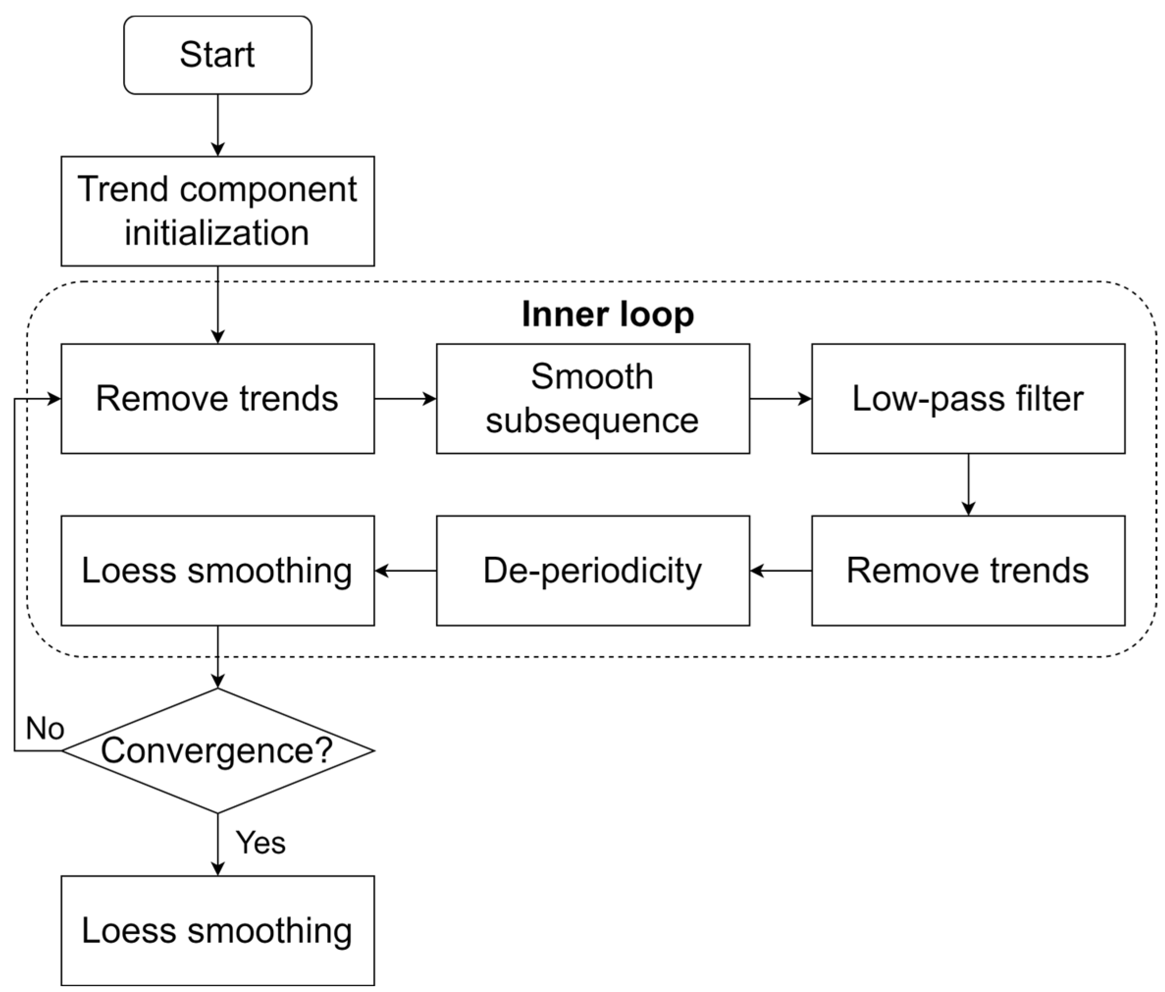
The STL algorithm (as shown in Figure 2) includes two parts: an outer loop and an inner loop. The Loess algorithm is used multiple times in the inner loop to smooth the trend and periodic components. The outer loop calculates robust weights based on the results of the inner loop to reduce the impact of noise on the next inner loop. Overall, the performance of the inner loop in the STL algorithm directly affects the generic performance in various scenarios and data features. The detailed procedure of the inner loop for STL is given as follows. Initialize the value in $T_t$ to 0, and set $Y_t$ as the original sequence. The steps of the inner loop are divided into the following 6 steps:

Step 1:

Remove trends. Generate $Y_t-T_t$ as a trend removal sequence.

Step 2:

Smooth subsequences. Firstly, the trend removal sequence is divided into multiple subsequences, and then each subsequence is smoothed with Loess. Then, each subsequence is combined and restored, and the restored sequence is defined as $C_t$.

Step 3:

Low-pass filtering on the restored sequence. The filtering process is divided into three steps:

Step 3.1:

First, two sliding averages with a cycle length.

Step 3.2:

One sliding average with a cycle length of 3.

Step 3.3:

Another Loess smoothing. Record the filtered result as $L_t$.

Step 4:

Remove trends. Generate a new periodic sequence as $S_t$, by $C_t$ minus $L_t$.

Step 5:

De-periodicity. Generate a new de-periodic sequence by $Y_t$ minus $S_t$.

Step 6:

Loess smoothing. Carry out Loess smoothing on the de-periodic sequence and obtain a new trend sequence $T_t$.

STL decomposition algorithm is a robust decomposition algorithm with a robust locally weighted regression algorithm to smooth the original time series data during the decomposition process, thereby overcoming the impact of outliers and missing values.

3.3. Periodic Factor Time Series Split Model

Many time series have obvious periodicity, such as shopping, passenger traffic, etc. For commuters, the traffic on Monday is the highest and the traffic on weekends is the lowest. Similar data shows a cyclical fluctuation trend, so it is necessary to consider cyclical factors and determine the length of the cycle, such as one week or one month, before making predictions.

For data with significant periodic fluctuations, the accuracy of using the ARIMA/Prophet model for prediction will decrease. The principle of ARIMA/Prophet is to use time points in the past to predict the next time point, which continues a trend. However, when applied to data with periodic factors, the prediction results will show significant deviation.

Therefore, the core task of using periodic factors to predict a time series is to extract periodic features, such as weekdays, as accurately as possible. The specific operation is to obtain the mean from Monday to Sunday, and then divide it by the overall mean to obtain the number of factors. The second step is to set a base, which can be the average of the last week. Finally, the base value is multiplied by the cycle factor for prediction. The specific process is given in Algorithm 1.

Algorithm 1: Periodic Factor Time Series Split Model

1. Segmenting the cycle: A cycle calculated based on one month is divided into each day as the unit of calculation.

2. Display frequency: Count the smallest unit of quantity and calculate the average over time.

3. Calculate cycle factor: Median factor, Weighting factor.

4. Prediction: Based on the cycle factor of each unit and the base, predict the minimum unit value.

5. Optimize Base: Optimizing the base is to optimize the average of the time period, by removing periodicity from the nearest unit values mentioned above, and then taking the average value.

It can be seen from the procedure that for time series data that are relatively stable and have strong periodicity without trend, time series prediction using periodic factors would be more reasonable.

3.4. LSTM-Wavelet Capital Predicting Model

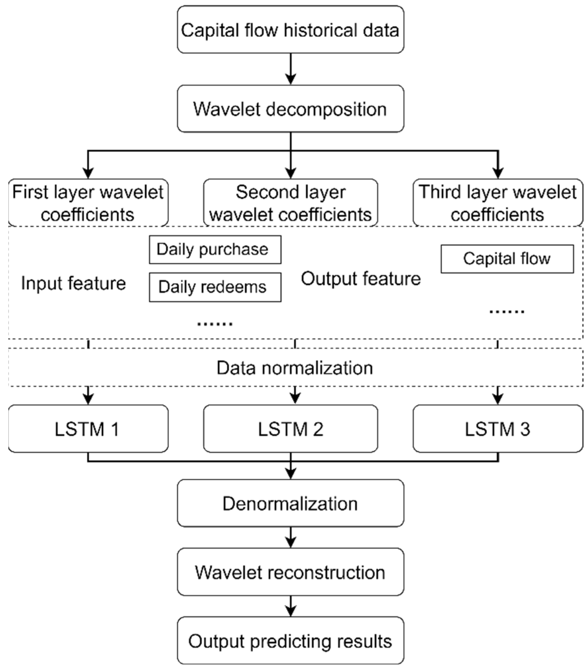
Due to high noise and severe data fluctuation characteristics in capital flow data, using the single neural network model to predict stock prices will easily lead to overlooking the impacts of different features on the output results. Therefore, this paper constructs an LSTM-Wavelet [35] model for capital prediction. It obtains wavelet coefficients with more obvious features through wavelet decomposition, and introduces the LSTM model for hierarchical prediction to achieve accurate prediction of capital flow. The introduced LSTM-Wavelet model can be implemented in three stages:

The first stage: wavelet decomposition is performed on the input dimensions of capital flow data to make the stabilized data more consistent with the original financial flow feature. Specifically, construct a subspace column within the subspace sequence space. If the subspace sequence has multi-resolution analysis, then for a given f(t):

$$f(t)={\displaystyle \sum _{m=m_0+1}^{\infty }{\displaystyle \sum _{n=-\infty }^{\infty }<f,{\Psi }_{m,n}>{\Psi }_{m,n}(t)}+}{\displaystyle \sum _{m=-\infty }^{m_0}{\displaystyle \sum _{n=-\infty }^{\infty }<f,{\Psi }_{m,n}>{\Psi }_{m,n}(t)}}$$

(17)

where ${\Psi }_{m,n}(t)=2^{-\frac{m}{2}}\Psi (\frac{t-n{2}^m}{2^m})=2^{-\frac{m}{2}}\Psi (2^{-m}t-n)$ is a binary discrete wavelet, $m\in Z$, and $n\in \Re$. The basis function of binary discrete wavelet ${\varphi }_{m,n}(t)$ is defined as Equation (18):

$${\varphi }_{m,n}(t)=2^{-\frac{m}{2}}\varphi (2^{-m}t-n)$$

(18)

where $m\in Z$ and $n\in \Re$. Set $C_{m_0,n}=<f,{\varphi }_{m,n}>,d_{m,n}=<f,{\Psi }_{m,n}>$, then Equation (17) can be transformed as Equation (19):

$$f(t)={\displaystyle \sum _{n=-\infty }^{\infty }{C}_{m_0,n}{\varphi }_{m,n}(t)}+{\displaystyle \sum _{m=-\infty }^m{\displaystyle \sum _{n=-\infty }^{\infty }{d}_{m,n}{\Psi }_{m,n}(t)}}$$

(19)

where the first part is the low-frequency part of f(t) at scale $2^{m_0}$, denoted as $A_{m_0}$, and the second part is the high-frequency part, denoted as $D_{m_0}$, so there is

$$A_{m_0-1}=A_{m_0}+D_{m_0}$$

(20)

$$f(t)=A_{m_0}+{\displaystyle \sum _{m=-\infty }^{m_0}{D}_m}=A_{m_0-1}+{\displaystyle \sum _{m=-\infty }^{m_0-1}{D}_m}$$

(21)

It can be seen from Equation (21) that multi resolution analysis only further decomposes the low-frequency part, whereas the high-frequency part is not considered.

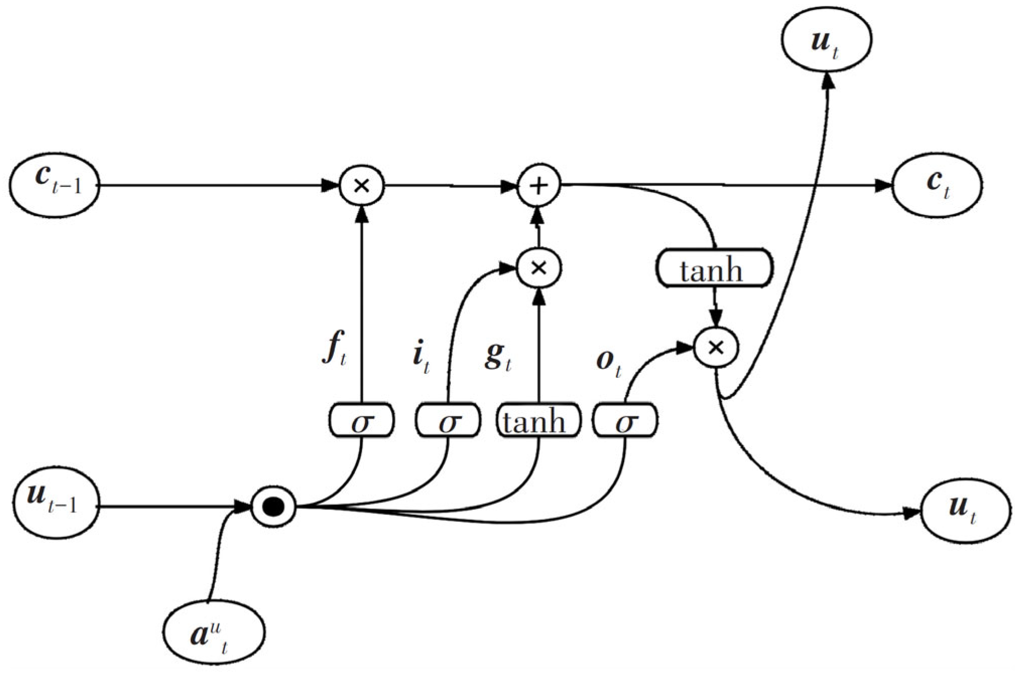
The second stage: LSTM models are established to predict the wavelet coefficients of each layer after wavelet decomposition. The LSTM neural network is a type of neural network commonly used for processing variable length sequences. The framework of LSTM is given in Figure 3.

LSTM solves gradient vanishing and explosion problems of traditional recurrent neural networks (RNNs), and adds gate (forgetting gate, input gate, output gate) settings to control the forgetting and updating of sequence information. After inputting the data ${\mathit{a}}_t^u$ into LSTM, it first enters the forgetting gate “and”, and through the sigmoid activation function the previous state information u_t−1 outputs the coefficient matrix f_t as

$${\mathit{f}}_{\mathit{t}}=\sigma ({\mathit{W}}_{\mathit{f}}\cdot [{\mathit{u}}_{t-1},{\mathit{a}}_t^u]+{\mathit{b}}_f)$$

(22)

where ${\mathit{W}}_f$ and ${\mathit{b}}_f$ represent the weight parameter matrix and bias parameter of the forgetting gate, respectively. Next, ${\mathit{a}}_t^u$ and u_t−1 enter the input gate and obtain the output ${\mathit{i}}_t$ through the sigmoid activation function. Then create a new value vector g_t by activating the tanh function with u_t−1 and ${\mathit{a}}_t^u$, and use the information from ${\mathit{i}}_t$ and ${\mathit{g}}_t$ to jointly control the update of sequence information as

$${\mathit{i}}_t=\sigma ({\mathit{W}}_i\cdot [{\mathit{u}}_{t-1},{\mathit{a}}_t^u]+{\mathit{b}}_i)$$

(23)

$${\mathit{g}}_t=\tanh ({\mathit{W}}_c\cdot [{\mathit{u}}_{t-1},{\mathit{x}}_t]+{\mathit{b}}_c)$$

(24)

where ${\mathit{W}}_i$ and ${\mathit{W}}_c$ represent the weight parameter matrices of the sigmoid and tanh activation function layers, respectively, and ${\mathit{b}}_i$ and ${\mathit{b}}_c$ represent the bias parameters of the sigmoid and tanh activation function layers, respectively. At this point, ${\mathit{c}}_{t-1}$ on the transmission belt outputs f_t through the forgetting gate, and completes the selective memory of the original sequence information. In addition, the product of the input gate output ${\mathit{i}}_t$ and the new value vector ${\mathit{g}}_t$ yields the new state information ${\mathit{c}}_t$, expressed as

$${\mathit{c}}_t={\mathit{f}}_t\times {\mathit{c}}_{t-1}+{\mathit{i}}_t\times {\mathit{g}}_t$$

(25)

After updating the forgetting gate and input gate, the data enters the output gate. The information of u_t−1 and ${\mathit{a}}_t^u$ are activated by the sigmoid function to obtain the output gate output o_t; Then, ${\mathit{c}}_{t-1}$ is combined with o_t through tanh transformation to obtain the final output u_t of the memory unit at that time, and transmitted to the next step as

$$\begin{array}{c}{\mathit{o}}_t=\sigma ({\mathit{W}}_o\cdot [{\mathit{u}}_{t-1},{\mathit{a}}_t^u]+{\mathit{b}}_o)\\ {\mathit{u}}_t={\mathit{o}}_t\cdot \tanh ({\mathit{c}}_t)\end{array}$$

(26)

where ${\mathit{W}}_o$ represents the weight parameter matrix of the sigmoid activation function layer, and ${\mathit{b}}_o$ represents the bias parameter of the sigmoid activation function layer.

The third stage: the predicted wavelet coefficients of each layer are reconstructed using wavelet to predict the capital flow. The framework of LSTM-Wavelet capital predicting model is shown in Figure 4.

3.5. Modeling Process

This paper proposed an automated capital prediction strategy of financial capital inflow and outflow using time series analysis artificial intelligence methods. First, to analyze the fluctuation and tail risk of financial characteristics, this paper explores the financial characteristics to measure the dynamic VaR from the perspectives of volatility, tail and peak with the Bayesian POT model. Next, in order to make the modeling more refined, the forecast targets are split with STL decomposition. Then, we construct a periodic factor time series split model to consider cyclical factors and to determine the length of the cycle. Finally, the time series modeling of the LSTM-wavelet model is carried out using a two-part analysis method to determine the linear separated wavelet and non-linear embedded wavelet parts to predict strong volatility in financial capital. The framework of the proposed method is given in Figure 5.

4. Results

The data for this study comes from the “Capital Flow Input/Output Prediction” competition provided by Alibaba Cloud, download at https://tianchi.aliyun.com/competition/entrance/231573/information (accessed on 1 March 2024). The dataset consists of four parts: basic user information data, user subscription and redemption data, the yield table, and the interbank lending rate table. This paper mainly uses the user subscription and redemption data table and the yield table, which records the operation of 28,000 users over 427 days. The operation record includes three parts: subscription, redemption, and yield information, and the unit of the amount is 0.01 yuan. The data has been desensitized to ensure safety, whilst the following calculation ensures there will be no negative value: Today’s Balance = Yesterday’s Balance + Today’s Subscription − Today’s Redemption.

The dataset used in this paper contains detailed information on the capital flow of Yu’e Bao. Due to the fact that the transaction records of a single user’s Yu’e Bao is recorded based on the user dimension, the usage behavior of a single user’s Yu’e Bao lacks regularity, and there are differences in financial management habits and consumption styles among different users, making it difficult to predict the fund flow of a single user. Based on this, the paper predicts and analyzes the transaction records of all users according to the dimension of date, that is, aggregating the transaction records of all users. The predicted analysis is the total daily purchase volume, total redemption volume, and yield volume of all users. We aggregate the dataset by date, add and process the same time, and calculate the total three attributes including purchase, subscription, and yield for each day.

In the analysis process, in order to clarify the fitting effect of the model and compare the calculation error with real data, it is necessary to divide the dataset into training data and test data. This article selects the data from the first 13 months (1 July 2013 to 30 July 2014) as the training set, and the data from the last month (August 2014) as the test set for model fitting. As the {subscription and redemption} and {yield} reflect different financial flow characteristics, the stability analysis is divided into two parts: (1) subscription and redemption, and (2) yield. First, extract the overall data of subscription and redemption information separately and visualize the calculated data as shown in Figure 6.

According to the risk analysis with the Bayesian POT model, the VaR test results are shown in

Table 1. Risk analysis results of Yu’e Bao’s return rate based on the Bayesian POT model.

Date	Original Return Rate	VaR Values at Different Confidence Levels
		90%	95%	97.50%	99%
1 January 2020	0.6618	2.036101	3.185459	5.516263	12.62633
2 January 2020	0.6616	2.034403	3.181464	5.507612	12.60347
3 January 2020	0.66	2.033131	3.178473	5.501134	12.58636
5 January 2020	1.319	2.028907	3.168536	5.479613	12.5295
6 January 2020	0.653	2.027643	3.165565	5.473178	12.5125
7 January 2020	0.6494	2.026802	3.163586	5.468893	12.50118
8 January 2020	0.652	2.025542	3.160622	5.462473	12.48422
9 January 2020	0.6498	2.02261	3.153724	5.447532	12.44474
10 January 2020	0.6834	2.018854	3.14489	5.428399	12.39419
12 January 2020	1.2902	2.013872	3.133172	5.403022	12.32715
13 January 2020	0.6796	2.013459	3.132199	5.400914	12.32158
14 January 2020	0.6792	2.013045	3.131226	5.398807	12.31601

. Under a given confidence level, the daily risk VaR value of Yu’e Bao’s return can be calculated. Due to space constraints, Table 1 only displays partial results. However, it can be observed that the higher the confidence level, the larger the VaR value. Moreover, by comparing the values in Table 1, it can be seen that (at a 90% confidence level) the VaR value estimated by the Bayesian POT model is already greater than its original rate of return, indicating the effectiveness of the Bayesian estimation.

After disassembling the time series using a statistical method (STL decomposition), visual analysis was performed on the total purchase data, as shown in Figure 7.

It can be seen from Figure 7 that the trend is consistently upward at the beginning, reaching a definitive peak and then beginning to decline. The initial trend is obvious, therefore the early stage belongs to a promotion period with a small number of users. However, in the later stage, as the number of users increases, it gradually stabilizes.

Due to the fact that yield is an important indicator for evaluating monetary funds and the main reason why investors are willing to buy, it is necessary to study the yield and risk of Yu’e Bao. After establishing a Bayesian POT risk measurement model from three perspectives including volatility, tail, and peak, the results are given as

Table 2. Basic statistical characteristics of Yu’e Bao yield series based on Bayesian POT method.

Mean	Standard	Deviation	Kurtosis	J-B Value (p-Value)
1.186	0.766	5.200	46.859	166,183.4

,

Table 3. Basic comparison of probability values under fixed interval length.

	$\mathit{\mu }\mathbf{\pm }\mathit{\sigma }$	$\mathit{\mu }\mathbf{\pm }2\mathit{\sigma }$	$\mathit{\mu }\mathbf{\pm }3\mathit{\sigma }$	$\mathit{\mu }\mathbf{\pm }4\mathit{\sigma }$
$p_1$	0.9022	0.9725	0.9852	0.9898
$p_2$	0.6827	0.9545	0.9973	0.9999
$p_3$	0.6824	0.9543	0.9973	0.9999

and

Table 4. Mode interval probability.

	${\mathit{S}}_1$	${\mathit{S}}_2$	${\mathit{S}}_3$
$M_0\pm \epsilon$	0.0041	0.0004	0.0004

with Basic statistical characteristics (including mean, standard, deviation, Kurtosis and J-B value, likely for the Jarque–Bera test (p-value) [38].

It can be seen from Table 2 that the deviation of the yield indicates that the yield exhibits an asymmetric distribution and a right skewed distribution; the kurtosis K > 3 indicates that the yield distribution has a peak characteristic. Based on the values of deviation and kurtosis, it can be found that the distribution of Yu’e Bao’s yield significantly rejects the assumption of a univariate normal distribution, which has sharper peaks than the normal distribution.

Overall, we can make the following conclusions from the data feature analysis results based on volatility, tail, and peak perspectives from Table 2, Table 3 and Table 4. For volatility, it was found that the previous volatility had a significant impact on the current volatility. For the tail information, the standard normal and t-distribution were used as comparison standards. After standardizing the yield data of Yu’e Bao with the same statistical caliber, the tail characteristics were explored. From tail length value and tail thickness value in Table 3, it was found that the Yu’e Bao sample data has longer and thinner tails; From the perspective of peak, according to the probability non-zero and probability distinguishability rules, it was found from Table 4 that the distribution of Yu’e Bao’s yield has sharper peaks. This indicates that the characteristics of yield are different from those of traditional financial product returns. Thus, the predicting model for yield must tolerate strong volatility. Based on the above three perspectives, due to the obvious periodic behavior, the periodic factor time series model was used.

Next, to demonstrate the effectiveness of the proposed model, a comparison of prediction results with the proposed method, the ARIMA [39] method, and the prophet [40] method for 32 days using the test dataset are given in Figure 8 and

Table 5. Comparison of prediction results for 32 days with the proposed model, ARIMA model, and the prophet model.

Model	Redeem		Purchase		Yield
	R2	RMSE	R2	RMSE	R2	RMSE
ARIMA	0.6290	0.5222	0.6091	0.5801	0.4183	1.3628
Prophet	0.7677	0.3497	0.7494	0.3959	0.4105	1.4210
Proposed model	0.8539	0.2406	0.8692	0.2318	0.8281	0.3002

. It can be seen from Figure 8 that the predicted results of the three models are relatively close to the real trend, but the predicting results of the ARIMA model and the prophet model are generally higher than the real values. In terms of the common lag in time series prediction, by comparing the predicted results of the three models with the observed values in the same trend position, it can be found that the proposed model is closest to the observed values in most cases of the same trend. It can be considered that the proposed model reduces a certain degree of lag compared to the compared two models, has a higher tolerance for data volatility, and is more consistent with the trend of changes in the observed values.

It can be seen from Table 5 that both the R² and root mean square error (RMSE) values of the proposed model are the highest, whereas the Prophet model also has a median model performance especially for the redeem and purchase data. The main reason for this is that the ARIMA time series model assumes stationary series modeling, whereas stock data has characteristics such as nonlinearity, non-stationary, and high noise. Whereas the wavelet decomposition decomposes the data into simpler structures and more obvious data trends, the proposed model can predict stock prices well. Moreover, due to the excellent ability of LSTM to extract detailed features, the proposed model applies the LSTM model to the hierarchical modeling of wavelet coefficients. Based on the characteristics of each layer’s coefficients, the total prediction results can be obtained through data fusion, resulting in more accurate prediction results and avoiding the overfitting problem.

5. Conclusions

To deal with the variability and significant nonlinearity of financial capital flows, this paper proposed an automated capital predicting model for the capital supply chain with Bayesian POT, Periodic factor, and LSTM Wavelet methods. By introducing wavelet decomposition, the LSTM model fully leverages its advantages. Modeling and predicting the wavelet coefficients of each layer separately not only effectively characterizes the nonlinearity of the data, but also reduces the impact of high noise factors. The experimental results show that the capital predicting model performs well in both volatility analysis and prediction performance. However, the mechanism and prior knowledge will be helpful for predicting the inflow and outflow of funds. For example, the understanding of outliers in data is currently attributed to festival factors, but in practice, the source of fluctuations, interest rates and other fluctuations may not be just festivals, and multi-channel positive and negative news will have an impact, which requires the experience and perception of front-line professional business personnel. In future work, to accurately evaluate the fluctuation of the inflow and outflow funds, the explainable mechanism and prior knowledge can be taken into account in the LSTM model.