Aerodynamic Performance and Numerical Analysis of the Coaxial Contra-Rotating Propeller Lift System in eVTOL Vehicles

Abstract

Electric vertical takeoff and landing (eVTOL) vehicles possess high payload transportation capabilities and compact design features. The traditional method of increasing propeller size to cope with high payload is no longer applicable. Therefore, this study proposes the use of coaxial counter-rotating propellers as the lift system for eVTOL vehicles, consisting of two coaxially mounted, counter-rotating bi-blade propellers. However, if the lift of a single rotating propeller is linearly increased without considering the lift loss caused by the downwash airflow generated by the upper propeller and the torque effect of the lift system, it will significantly impact performance optimization and safety in the eVTOL vehicles design process. To address this issue, this study employed the Moving Reference Frame (MRF) method within Computational Fluid Dynamics (CFD) technology to simulate the lift system, conducting a detailed analysis of the impact of the upper propeller’s downwash flow on the aerodynamic performance of the lower propeller. In addition, the aerodynamic performance indicators of coaxial counter-rotating propellers were quantitatively analyzed under different speed conditions. The results indicated significant lift losses within the coaxial contra-rotating propeller system, which were particularly notable in the lift loss of the lower propeller. Moreover, the total torque decreased by more than 93.8%, and the torque was not completely offset; there was still a small torsional effect in the coaxial counter-rotating propellers. The virtual testing method of this study not only saves a significant amount of time and money but also serves as a vital reference in the design process of eVTOL vehicles.

1. Introduction

As the number of personal vehicles in use worldwide surges, this trend has not only intensified climate change but also led to increased congestion within major urban regions, making urban air mobility an emerging market for aerial transportation systems [1,2]. Flying cars, especially electric vertical takeoff and landing (eVTOL) vehicles, with their zero-emission advantage, are considered an innovative solution to address future urban traffic congestion and environmental issues [3,4]. However, the design and implementation of eVTOL vehicles face various challenges, one of which is their size limitation. Due to the complexity and spatial constraints of urban environments, the size of eVTOL vehicles needs to be meticulously designed to ensure they can fit into parking spaces [5]. Therefore, developing compact flying car designs suitable for urban environments is a key task.

The coaxial contra-rotating propellers comprise two closely positioned propellers that rotate in opposite directions around the same axis. This configuration is designed to achieve higher propulsion speeds and superior thrust efficiency compared to using a single propeller [6,7]. Based on this advantage, coaxial counter rotating propellers have been widely used in the field of unmanned aerial vehicles (UAV) [8,9]. As the core component of the lift system for eVTOL vehicles, the aerodynamic performance of coaxial counter-rotating propellers plays a decisive role in the overall performance and safety of eVTOL vehicles [10]. Therefore, a deep understanding and accurate simulation of the aerodynamic interactions between coaxial counter-rotating propellers and the precise evaluation of their aerodynamic performance are crucial factors that need to be considered in the design process of eVTOL vehicles.

eVTOL vehicles are an innovative mode of transportation. Although the design technology of eVTOL vehicles is rapidly advancing, conducting low-cost, efficient, and high-precision quantitative analysis of the aerodynamic performance of the coaxial contra-rotating propeller lift system remains a challenge in the design process of eVTOL vehicles. eVTOL vehicles often require a significant investment of time and money in the verification process before they can be officially put into operation. Previous development commonly adopted a method of repeated iterations of prototype design and testing, a practice that not only consumed a considerable amount of time but also incurred high costs [11]. With the theoretical development of the propeller design field, analysis methods such as the blade element theory (BET), the blade element momentum theory (BEMT), or the free vortex method (FVM) have been considered as reliable methods for the design and performance testing of propellers due to their high speed [12,13,14,15,16]. However, this method requires input parameters in the experiment to produce accurate results, making it difficult to use them to accurately evaluate new designs without additional experimental research. Given the complexity of aerodynamic interactions in coaxial counter-rotating propellers, traditional analysis methods often fall short in capturing the intricate flow dynamics and providing accurate performance predictions. This limitation underscores the need for more advanced and precise tools. Computational fluid dynamics (CFD) methods, due to their extensive modeling capabilities and accurate verification methods, are increasingly being explored by researchers for their application in propeller design and analysis. The CFD approach, through numerical simulation techniques, enables the precise prediction of the aerodynamic characteristics of propellers, avoiding repetitive experiments and modifications common in traditional prototype testing. Moreover, CFD methods also provide more in-depth flow field analysis, offering robust support for the optimization of the lift system in eVTOL vehicles. Mohamed [17] conducted a study on the slotted propeller design for different airfoils using the MRF method in CFD to improve the aerodynamic performance of small propellers. Dubbioso [18] assessed the performance of marine propellers under off-design conditions, focusing on hydrodynamic loads and pressure distribution on the blades. Liu [19] systematically analyzed the aerodynamic performance of the APC1045 multi-rotor propeller through wind tunnel tests, blade element momentum theory, and CFD methods, exploring the limitations and advantages of these three methods. Oktay [20] used the overlapping grid method in CFD to investigate the relationship between the airspeed and thrust coefficient of a quad-rotor UAV propeller, with the results indicating that the thrust coefficient decreases at higher airspeeds. Rajendran [21] conducted a numerical simulation analysis to investigate the effects of blade angle on the torque generated by twin-blade propellers and developed a twin-blade propeller model with improved torque and performance coefficient. Trimulyono [22] studied the effect of installing propeller boss cap fins on propeller performance using the CFD method. Additionally, Trimulyono [23] also employed the model variation analysis method to study the optimum thrust value of the propeller, as well as the thrust values generated by variations in angle and number of blades. Fitriadhy [24] studied the thrust, torque, and efficiency coefficients of propellers with different blade numbers in open-water conditions using the CFD method. Guo [25] used CFD and system-based methods to study the turning maneuver behavior and hydrodynamic characteristics of twin-screw ships considering hull-engine-propeller interaction, but the research object was different from the aerodynamic characteristics of coaxial contra-rotating propellers discussed in this paper.

However, the CFD simulation in the above research is all for single propeller, and the aerodynamic interaction of coaxial counter-rotating propeller used in eVTOL vehicles is extremely complex [26], especially the impact of the downwash generated by the upper propeller on the lower propeller, which makes the aerodynamic performance of this lift system exhibit complex and variable characteristics, which are difficult to predict directly [27]. Sugawara [28] studied a CFD numerical simulation method combined with balance analysis. Through the balance analysis loosely coupled with the CFD solver, the blade pitch angles of the upper and lower rotors were adjusted to meet the target balance conditions. Wang [29] simulated the aerodynamic characteristics of coaxial propellers within a duct for eVTOL aircraft by establishing a sliding mesh model, analyzing the lift and torque of the ducted coaxial propellers at different speeds. However, the structure of the lift system differs from that presented in this paper. Lei [30] and Park [31], respectively, employed the sliding mesh and the overset mesh to analyze the impact of rotor spacing on the aerodynamic characteristics, thrust, and power consumption of coaxial propellers through numerical simulation. These results demonstrated the variations in rotor interference and thrust coefficient with increasing rotor spacing. However, the main focus of their research was not the analysis of lift losses and torque changes at different rotational speeds. Vijayanandh [32] studied the cumulative thrust of the coaxial propeller in compact size, and the thrust and stability are optimized by modifying the distance between coaxial propellers. Cornelius [33] developed a blade-resolved approach using mixing plane boundaries to analyze the aerodynamic performance of multi-rotor UAV systems, achieving a reduction in computational time and grid cell count by $99.8\%$ and $48.3\%$, respectively.

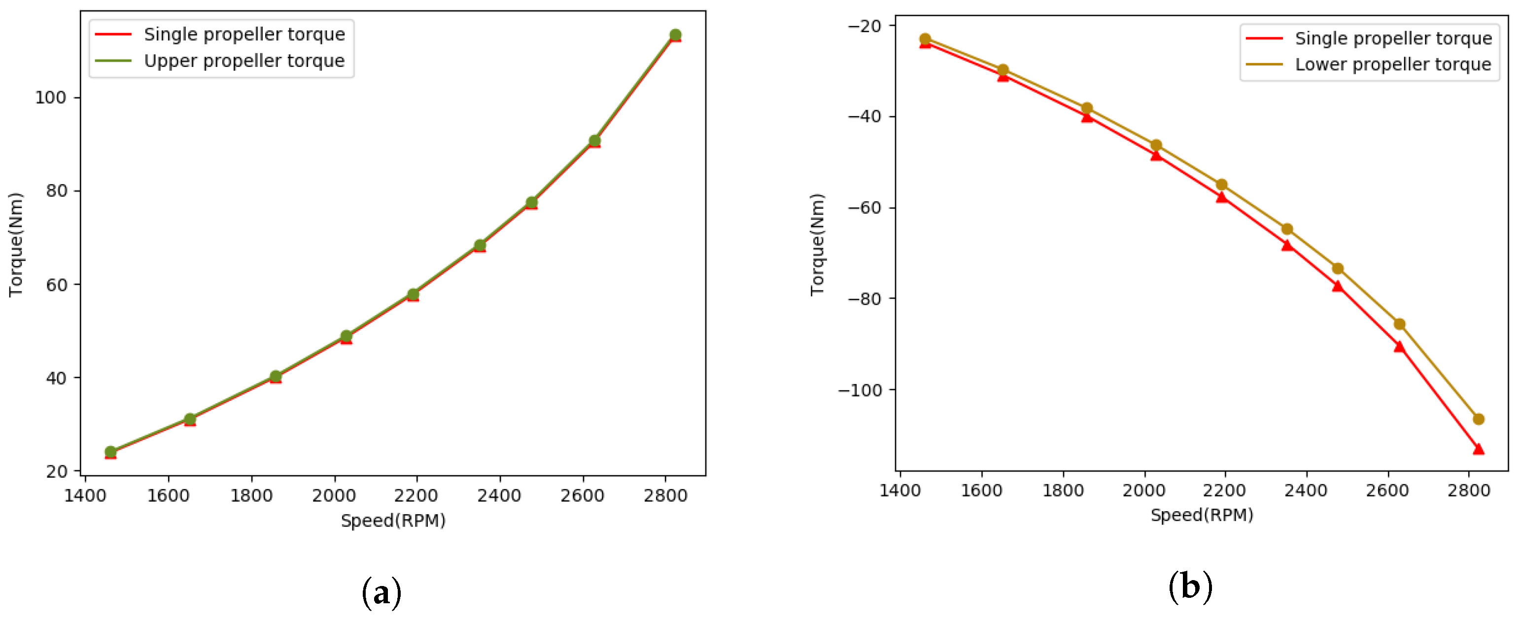
Currently, the numerical simulation studies of coaxial propellers are mostly focused on spacing optimization, while the quantitative analysis of lift loss and torque variation at different rotational speeds, as well as coaxial interference analysis, are still insufficient. In the design optimization process of eVTOL vehicles, considering both the total lift loss and torque variation is essential to ensure high performance and safety. Insufficient consideration of lift loss could lead to the design of eVTOL vehicles that fail to meet expected performance standards, such as specific payload requirements or flight altitude limitations. Meanwhile, in the ideal case of coaxial counter-rotating propellers, the torque generated by the upper and lower propellers should be balanced to achieve mutual cancellation [34,35]. If the variation in torque is not adequately assessed, it may lead to undesirable rotations or oscillations of the aircraft, increasing uncertainty and risk during flight. Therefore, an efficient research method for studying the lift loss and torque variation of coaxial counter-rotating propellers at different rotational speeds is crucial for the design process of eVTOL vehicles.

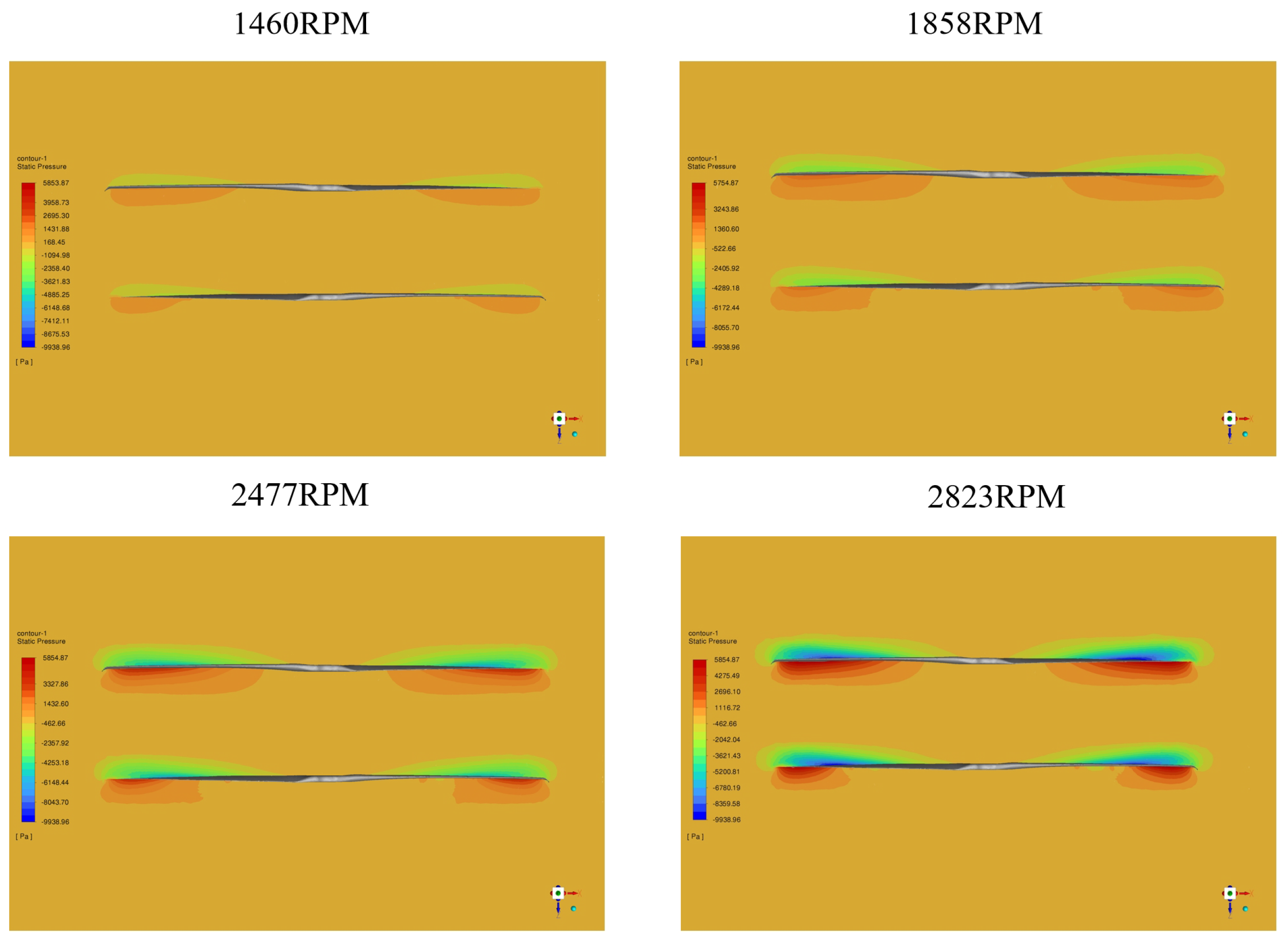
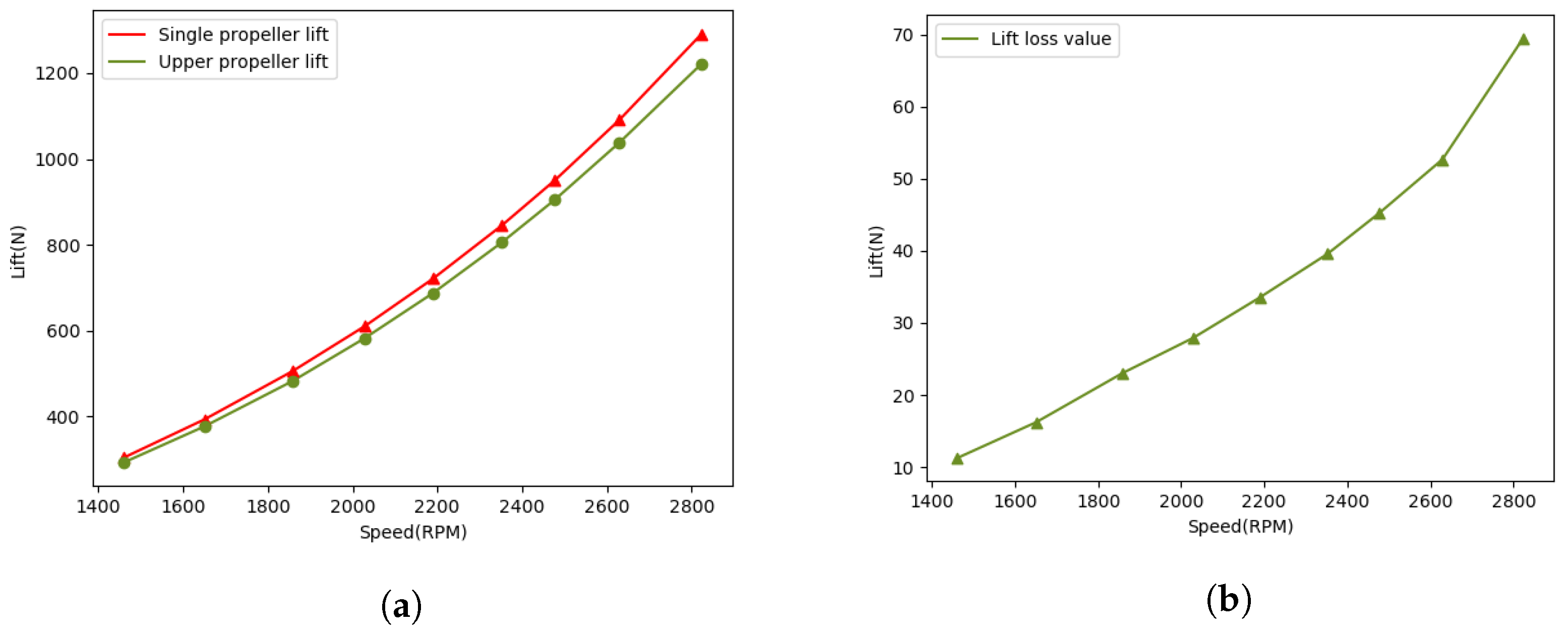
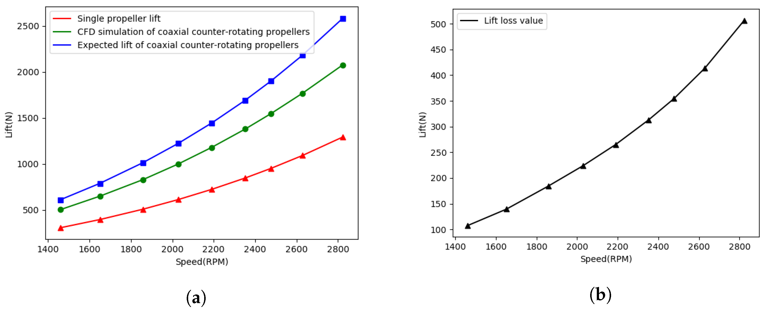
In response to the challenges identified in the design optimization of eVTOL vehicles, this article employs the MRF method in CFD technology to numerically simulate the lift system, providing a detailed analysis of the impact of the upper propeller’s wake flow field on the aerodynamic performance of the lower propeller. Additionally, it quantitatively analyzes the lift loss and torque variation of the coaxial counter-rotating propellers under different rotational speed conditions. This method does not require any hardware, making it a virtual test for the lift system of eVTOL vehicles, which can be used to estimate the dynamic loads on the lift system. This approach can serve as an important reference for performance optimization and safety during the design process of eVTOL vehicles.

2. Problem Statement

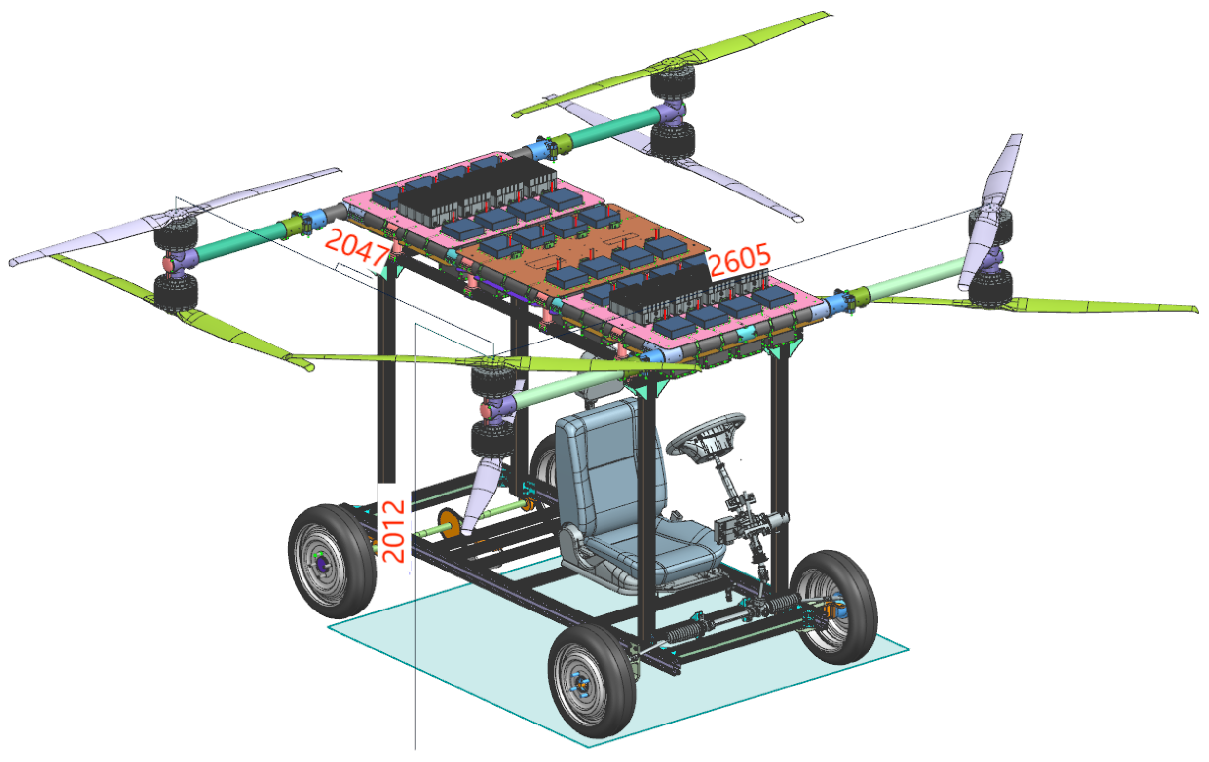
Figure 1 presents the quad-rotor, octa-propeller configuration of the flight system for the flying car discussed in this paper. This configuration not only provides ample power for the flight of the flying car but also meets the safety requirements of power redundancy. The flying car’s expanded dimensions are 2605 mm in length, 2047 mm in width, and 2012 mm in height. The power system of the aircraft consists of 24 distributed 12S44 Ah battery packs, arranged atop the vehicle’s body, which is advantageous for heat dissipation and enhancing the vehicle’s center of gravity, thereby reducing the moment of inertia and easing the operation difficulty. The fixed mass of the flying car is as shown in

Table 1. Fixed mass of flying car system.

Component Type	Mass (Kg)	Quantity	Total Mass (Kg)
Power system	13	8	104
Battery	180	1	180
Frame	70	1	70
Flight Control/Data Transmission/GPS	0.5	1	0.5
Other Electronic Components and Circuits	2	1	2

, which includes specific hardware components and core mechanical parts. The total weight of this part remains essentially constant, whereas the quantity or materials of other components not listed in the table can be adjusted according to requirements.

Following the design criteria for the flying car outlined above, this study delves into the power system of the flying car. Considering the high payload requirements and the need for a compact airframe in practical applications, the traditional method of increasing propeller size to enhance lift is no longer viable. Therefore, this research employs a coaxial counter-rotating propeller system designed to provide greater lift without significantly increasing the dimensions of the flying car.

For a quadrotor unmanned aerial vehicle (UAV) with inter-axial angles set at ${90}^{\circ }$ and propeller sizes of 67 inches, the body’s axis radius R is related to the maximum rotor radius $r_{max}$ as follows:

$$\mathrm{R}=\frac{1}{sin\left({90}^{\circ }/2\right)}{\mathrm{r}}_{max}$$

(1)

where ${\mathrm{r}}_{max}=1.05{\mathrm{r}}_{\mathrm{p}}$∼$1.2{\mathrm{r}}_{\mathrm{p}}$, $r_p$ is the propeller radius, and its value is 850.9 mm. This yields $r_{max}$ values between 893.45 mm and 1021.08 mm. Consequently, the range of R extends from 1263.4 mm to 1443.81 mm.

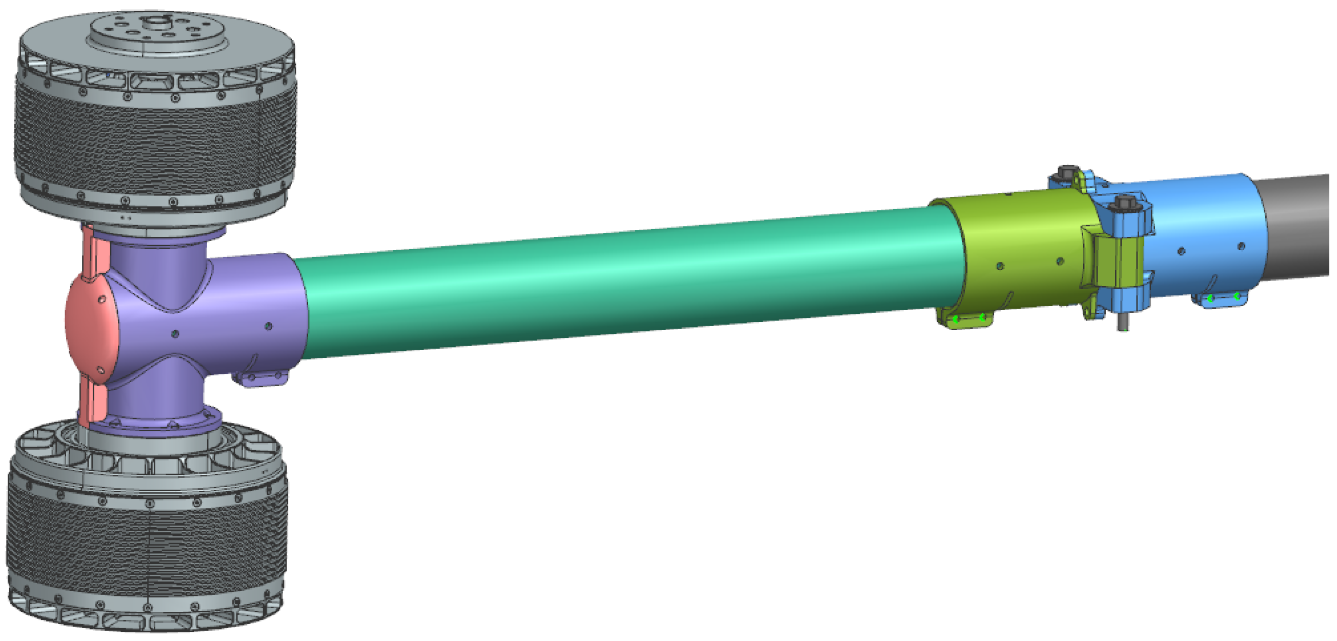
The motor model is EA200, with external dimensions of $⌀195.4\times 120\mathrm{mm}$. The propeller arm assembly consists of the arm fixture, carbon tube, and motor mount, as illustrated in Figure 2. The arms can be regarded as cantilever beams. In this study, the distance between the two propellers is set at 420 mm.

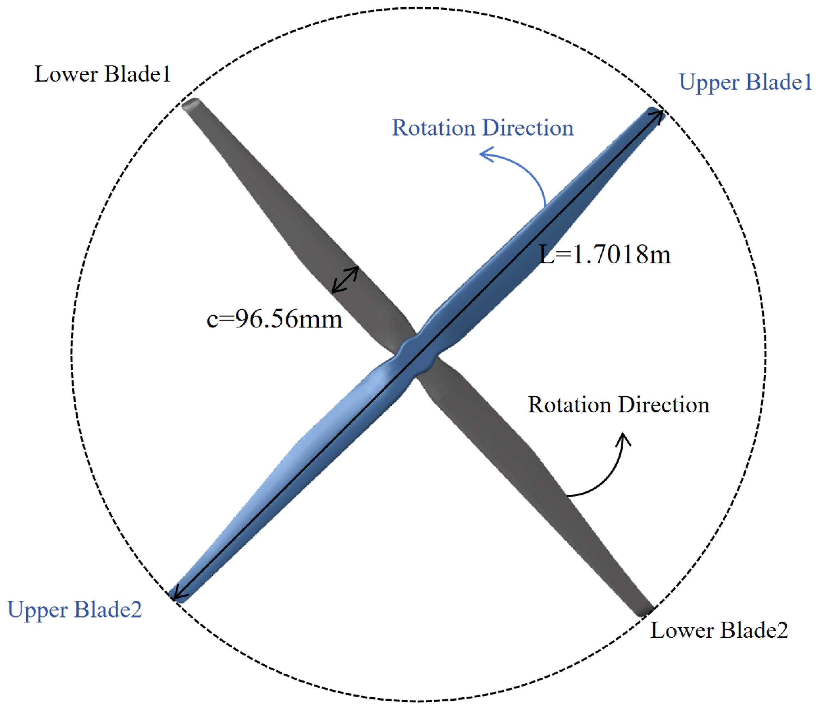
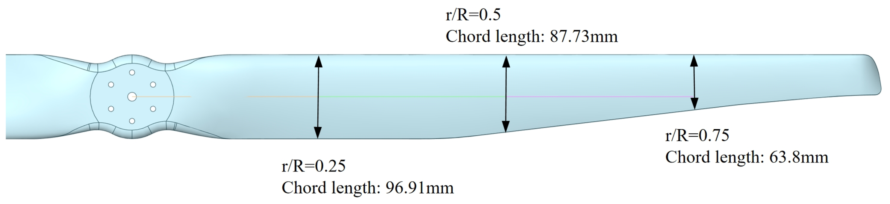
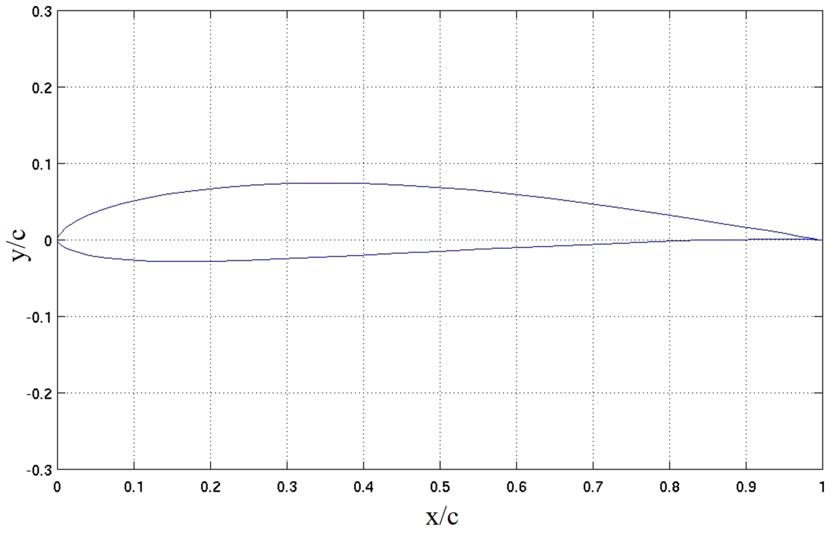
This paper primarily investigates a set of coaxial contra-rotating propellers within the lift system, utilizing coaxial contra-rotating propellers as shown in Figure 3, which consist of two propellers rotating in opposite directions. In the lift system of the flying car, there are two sets of coaxial contra-rotating propellers whose rotation direction is the same as that shown in Figure 3, while the other two sets utilize propellers with the opposite rotation direction. The propeller is designed with mh117 basic airfoil as shown in Figure 4, and the detailed dimensions are shown in Figure 5. The parameters related to the coaxial counter-rotating propellers are presented in

Table 2. Propeller parameters.

Parameters	Value
Diameter (m)	1.7018
Spacing between propellers (m)	0.42
Maximum Blade Chord Length (m)	0.09656
Average Blade Chord Length (m)	0.07476
Number of blades	2
Material of blades	Carbon fiber
Weight (kg)	0.85
Pitch (mm)	11.34
Maximum speed (RPM)	3000

.

3. Computational Model and Numerical Method

In comparison to individual propellers, coaxial counter-rotating propellers suffer from aerodynamic interference, resulting in a reduction in lift; hence, the total lift of the flying car’s lift system cannot be simply deduced by summing the lift produced by two separate propellers. At the same time, it is also necessary to analyze whether the torque effect still exists in the coaxial counter-rotating propeller. The CFD method can provide detailed flow field information, including but not limited to velocity fields, pressure distribution, and vortex structures, enabling an in-depth analysis of the aerodynamic interactions of coaxial counter-rotating propellers. Furthermore, the CFD method can also accurately predict lift loss and torque variations. In order to analyze the lift loss and torque variation of coaxial counter-rotating propellers at different speeds, the theoretical and control equations used in this paper are first introduced in Section 3.1. Section 3.2 describes grid generation and sets the solution conditions. Perform grid independence verification to ensure accuracy in calculating lift while considering computational efficiency. Finally, the CFD simulation results were compared with the experimental data provided by the propeller manufacturer to verify the accuracy of the model.

3.1. Numerical Method

The propeller’s lift coefficient $C_T$ and torque coefficient $C_M$ are as follows:

$$C_T=T/\rho n_s^2{D}^4$$

(2)

$$C_M=M/\rho n_s^2{D}^5$$

(3)

where T is the lift, M is the torque, $\rho$ is the air density, $n_s$ is the rotational speed, and D is the propeller diameter. When two counter-rotating propellers are arranged coaxially, the outflow of the upper propeller is directed into the inflow of the lower propeller, affecting the total lift of both propellers. The formula for calculating the total lift $T_{sum}$ of coaxial counter-rotating propellers is as follows:

$${\mathrm{T}}_{sum}=T_1+T_2=C_{T1}\rho D^4{n}_{s1}^2+C_{T2}\rho D^4{n}_{s2}^2$$

(4)

where $T_1$ and $T_2$ are the lift of the upper propeller and lower propeller, $C_{T1}$ and $C_{T2}$ are the lift coefficients of the upper propeller and lower propeller, $n_{s1}$ and $n_{s2}$ are the rotational speeds of the upper propeller and lower propeller, respectively. In this paper, $n_{s1}=n_{s2}$.

3.1.1. Fluid Dynamics

The Reynolds number is a dimensionless metric used to characterize the nature of fluid motion around a propeller [36]. It represents the ratio of inertial forces to viscous forces within the fluid flow, and the formula for calculating the Reynolds number of a propeller is as follows:

$$Re=\frac{\rho c_{0.75R}\sqrt{v^2+{\left(0.75\pi n_{s}D\right)}^2}}{\mu }$$

(5)

where $\rho$ is the fluid density, $c_{0.75R}$ represents the chord length at the 0.75R section of the blade, and $\mu$ is the dynamic viscosity of the fluid. v represents the velocity of the fluid relative to the propeller’s blade, and in this study, the aerodynamic characteristics of the propeller in a hover state are investigated; thus, $v=0$. The range of $n_s$ is from 1460 RPM to 2823 RPM, and the propeller Reynolds number is between $5\times {10}^5$ and $8.3\times {10}^5$, indicating complex turbulent flows that necessitate the selection of a turbulence model for resolving the turbulence in the flow field.

Due to the presence of turbulence in the flow field around coaxial contra-rotating propellers, it is impractical to resolve the actual flow by setting extremely fine meshes and very small time steps in the solving process. Therefore, when simulating turbulent fluctuations, the Reynolds-Averaged Navier–Stokes (RANS) method based on the Finite Volume Method (FVM) is used to solve for the average flow rate [37]. The derivation of the RANS equations is detailed in [38].

In the RANS formulation, it is necessary to approximate the Reynolds stress terms by employing turbulence models, thereby providing a closed form that renders the RANS equations solvable. Currently, the $k-\omega$ Shear Stress Transport (SST) turbulence model has been widely applied to the numerical simulation studies of propellers [39,40,41]. Firstly, compared to the conventional $k-ϵ$ model, the $k-\omega$ SST model provides more accurate predictions for the flow close to walls, which is crucial for the study of propeller performance as the complex flow field around propellers often involves various flow phenomena, including the formation of shear layers and flow separation. Secondly, although the original $k-\omega$ model excels near wall regions, it has shortcomings in free-stream regions away from walls. The $k-\omega$ SST model overcomes this by blending the strengths of the $k-\omega$ model near the wall with the advantages of the $k-ϵ$ model in far-field flows. Moreover, the introduction of the cross-diffusion term in the $k-\omega$ SST model significantly enhances its applicability across different flow regions, thereby increasing the model’s robustness [42,43]. For this task, we have chosen the $k-\omega$ SST turbulence model.

3.1.2. $k-\omega$ SST Turbulence Model

When constructing the $k-\omega$ SST model, the $\omega$ transport equation plays a central role. It describes the temporal variation of the specific dissipation rate of turbulence kinetic energy, $\omega$, as well as its transport within the fluid. The equation is as follows:

$$\begin{array}{c}\frac{\partial \left(\rho \omega \right)}{\partial \mathrm{t}}+div\left(\rho \omega \mathrm{U}\right)=div\left[\left(\mu +{\sigma }_{\omega }{\mu }_{\mathrm{t}}\right)grad\left(\omega \right)\right]+\gamma \rho {\mathrm{S}}^2-\beta \rho {\omega }^2\hfill \\ +2\left(1-F_1\right){\sigma }_{\omega }\frac{\rho }{\omega }\frac{\partial k}{\partial x_i}\frac{\partial \omega }{\partial x_i}\hfill \end{array}$$

(6)

where ${\mu }_{\mathrm{t}}$ represents the turbulent viscosity coefficient, and ${\sigma }_{\omega }$ is the turbulence Prandtl number, which is an empirically derived dimensionless coefficient used to correct the diffusion of turbulence quantities. The modeling coefficients $\gamma$ and $\beta$, respectively, correspond to the production and dissipation terms. The last term on the right side is the cross-diffusion term, which does not exist in the original $k-\omega$ model. $F_1$ is a blending function designed to smoothly transition between the near-wall region and the region far from the wall; it approaches 1 near the wall (activating the $k-\omega$ model) and goes to 0 away from the wall (activating the $k-ϵ$ model). The weight of this term is adjusted by $F_1$ based on the flow field’s position, ensuring the model maintains high accuracy both near and far from the wall surfaces.

The transport equation for turbulence kinetic energy k is as follows:

$$\frac{\partial \left(\rho \mathrm{k}\right)}{\partial \mathrm{t}}+div\left(\rho \mathrm{k}U\right)=div\left[\left(\mu +\frac{{\mu }_{\mathrm{t}}}{{\sigma }_{\mathrm{k}}}\right)grad\left(\mathrm{k}\right)\right]+{\mathrm{P}}_k-{\beta }^{*}\rho k\omega$$

(7)

The second term, ${\mathrm{P}}_k$, is the production term, and the final term represents the dissipation, where ${\beta }^{*}$ is a constant set to the standard value of 0.09 [42].

3.2. Computational Model

3.2.1. Mesh Generation

The computational simulation of the coaxial counter-rotating propellers was carried out using the computational fluid dynamics software ANSYS Fluent 19.0. Initially, an unstructured mesh for the flow domain and rotational domain of the propellers was generated using Fluent-Meshing. As shown in Figure 6, the lift system is positioned 5.3 m from the inlet and 12 m from the outlet. To accurately simulate the flow around the coaxial counter-rotating propellers, two mesh refinement zones were established—Encryption Zone 1 being fine and Encryption Zone 2 being finer—ensuring both computational precision for the lift system and overall computational efficiency. The fluid domain is partitioned into a steady region and rotating regions (with distinct rotating zones for the upper and lower propellers), where the rotating regions are cylindrical areas with a diameter 1.1 times that of the propeller diameter and a thickness of 0.15 m. To simulate wind tunnel tests, the stable zone is modeled as a cylinder with a height of 18 m and a base radius of 6 m. Within this stable zone, Mesh Encryption Zone 1 and Mesh Encryption Zone 2 are incorporated as integral parts of the domain. The number of mesh cells in the flow field domain is 2,000,427; the number of mesh cells in the upper propeller rotation domain is 191,394; and the number of mesh cells in the lower propeller rotation domain is 191,394.

In this study, the stationary and rotating domains are divided using tetrahedral meshing, as depicted in Figure 7a,b. The propeller surface is meshed with a combination of quadrilateral and triangular elements, as illustrated in Figure 8a. The boundary layer surrounding the coaxial counter-rotating propellers has a significant impact on the aerodynamic performance of the flying car’s lift system. To accurately resolve the boundary layer and capture its influence on the airflow induced by the propellers, the mesh is refined in the vicinity of the propeller surfaces. In the numerical simulation of the aerodynamic characteristics of propellers, the non-dimensional wall distance $y^{+}$ is directly related to the refinement of the grid near the wall. Choosing an appropriate $y^{+}$ value is crucial for accurately capturing the subtle features of the interaction between the propeller blades and the fluid. In this study, the $y^{+}$ value for the first layer of grid nodes is set to 1 to ensure accurate simulation of the turbulence characteristics near the wall. The boundary layer mesh is shown in Figure 8b.

3.2.2. Solving Condition

In order to precisely simulate the dynamic behavior of coaxial counter-rotating propellers and the complex flow field surrounding them, we have utilized a combined application of Multiple Reference Frame (MRF) technology and overlapping grid techniques. The MRF approach sets a uniform rotational velocity within the rotating domain relative to the propeller rotation, achieving a steady-state approximation of the propeller’s rotation. This method reduces the demand on computational resources while maintaining sufficient accuracy in the simulation. The overlapping grid technique, on the other hand, is employed to manage the interfaces between dynamic regions, allowing independent rotation of different grid systems without disturbing the mesh structure of the static domain. By facilitating detailed exchange of information within the overlap regions, it captures the non-linear fluid effects and complex flow variations induced by the rotation of the propellers.

The air density is set to $1.225\mathrm{kg}/{\mathrm{m}}^3$ with a viscosity of $1.7895\times {10}^{-5}\mathrm{Pa}·\mathrm{s}$. The velocity inlet is set to 0 m/s, and the propeller wall boundary condition is defined as a Moving Wall, rotating around the z-axis at a speed of 1460 RPM to 2823 RPM. The Coupled algorithm is employed for pressure-velocity coupling, ensuring a robust and efficient solution. Momentum is discretized using a Second Order Upwind scheme, and Turbulent Kinetic Energy is also treated with a Second Order Upwind approach [44]. The second-order upwind schemes offer higher accuracy compared to first-order schemes and are better suited for capturing complex flow characteristics. The detailed parameters for solving the conditions are shown in

Table 3. Solving condition parameters.

Item	Type	Pressure (Pa)	Velocity (m/s)	Rotational Speed (RPM)
Inlet	Velocity-inlet	101,325	0	-
Outlet	Pressure-outlet	101,325	-	-
Wall	Stationary wall	-	-	-
Upper rotation region	Fluid	-	-	1460–2823
Lower rotation region	Fluid	-	-	1460–2823
Turbulence Model	$k-\omega$ SST	-	-	-
Upper propeller	Moving wall	-	0	0
Lower propeller	Moving wall	-	0	0

.

3.2.3. Mesh Independence Verification

In this study, grid convergence was validated at a rotation speed of 2029 RPM. The Grid Convergence Index (GCI) is a method based on Richardson extrapolation to measure the error between different levels of grid refinement, and we applied it to the grid convergence verification in this paper [45,46]. The formula for calculating GCI is as follows:

$${\epsilon }_{i,i+1}=\frac{|f_{i+1}-f_i|}{f_i}$$

(8)

$$GC{I}_{i,i+1}=F_s\frac{{\epsilon }_{i,i+1}}{r_{i,i+1}^p-1}$$

(9)

where $F_s$ serves as the safety factor, with a value of 1.25 typically used for three-grid verification. ${\epsilon }_{i,i+1}$ represents the error estimate between the fine and the coarse grids; p signifies the order of convergence; and r is the grid refinement ratio, which does not require a fixed value [47]. The values for $r_{12}$ and $r_{23}$ are 1.21 and 1.24, respectively. The GCI calculation results are presented in

Table 4. Mesh independence verification results.

Type	Number of Cells	Upper Propeller			Lower Propeller
		${\mathit{T}}_{\mathbf{1}}$(N)	${\mathit{\epsilon }}_{\mathit{i},\mathit{i}+\mathbf{1}}$	${\mathit{GCI}}_{\mathit{i},\mathit{i}+\mathit{1}}$	${\mathit{T}}_{\mathbf{2}}$(N)	${\mathit{\epsilon }}_{\mathit{i},\mathit{i}+\mathbf{1}}$	${\mathit{G}\mathit{C}\mathit{I}}_{\mathit{i},\mathit{i}+\mathbf{1}}$
Coarse	1,324,711	558.866			396.382
			4.31%	11.61%		4.67%	12.5%
Medium	2,383,215	582.956			414.892
			0.37%	0.86%		0.39%	0.9%
Fine	4,549,275	585.120			416.504

. It can be seen that the value of $GC{I}_{23}$ is relatively small, suggesting that the computational results on the medium mesh are already nearing the ideal performance for coaxial contra-rotating propellers. Taking computational efficiency into account, this study is conducted based on the medium mesh.

3.2.4. Comparison of Experimental Results and CFD Simulations

In this paper, the CFD simulation results are compared with the experimental data provided by the propeller manufacturer using the single propeller model introduced in Section 2. Figure 9a,b present a comparison of lift and torque between CFD simulation and experimental results within the rotational speed range of 1460 RPM to 2823 RPM, with the simulation results closely matching the actual test values. The specific values and errors are shown in

Table 5. Comparison of single propeller CFD simulation results with experimental data.

Speed (RPM)	CFD Simulation		Experimental Result		$\mathbf{\Delta }\mathit{T}$	$\mathbf{\Delta }\mathit{M}$
	T (N)	M (Nm)	T (N)	M (Nm)
1460	304.528	23.889	311.985	26.024	−2.38%	−8.20%
1651	393.849	30.989	407.625	32.092	−3.38%	−3.44%
1858	505.719	39.974	531.448	39.773	−4.8%	0.51%
2029	610.887	48.535	637.434	47.072	−4.16%	3.11%
2190	721.433	57.676	749.739	54.594	−3.78%	5.65%
2352	845.155	68.127	864.644	63.876	−2.25%	6.65%
2477	950.182	77.276	990.153	73.718	−4.04%	5.40%
2629	1090.363	90.457	1146.240	84.989	−4.87%	6.43%
2823	1226.109	107.185	1282.147	101.127	−4.37%	5.99%

, with the maximum lift error not exceeding $5\%$ and the maximum torque error not exceeding $8.2\%$, demonstrating the credibility of the CFD model.

4. Result and Analysis

4.1. The Impact of Upper Propeller Downwash on the Aerodynamic Performance of the Lower Propeller

In this study, the rotational behavior of a propeller in a quiescent air environment is considered. The inflow generated by the rotating propeller interacts with the induced rotational wind speed, collectively defining the dynamic airflow encountered by the propeller during operational conditions. The region upstream of the propeller, significantly influenced by the rotation, is designated as the inflow zone. This inflow zone transitions into the outflow zone after passing through the propeller, subsequently forming the distinctive downwash flow region beneath the propeller.

We delved into the flow characteristics and pressure distribution of both upper and lower propellers in a coaxial counter-rotating propeller system. Figure 10 shows the velocity distribution of the coaxial contra-rotating propellers. It can be observed that, as the rotational speed increases, the downwash airflow from the upper propeller interacts more complexly with the airflow generated by the lower propeller. This interaction leads to alterations in the flow field structure of the lower propeller, thereby directly impacting its performance. To clearly display the aerodynamic differences between the two propellers, we present the pressure contour maps of the flow field cross-section around the coaxial counter-rotating propellers at rotational speeds ranging from 1460 RPM to 2823 RPM, as shown in Figure 11. From the pressure cloud map of the lower surface of the propellers shown in Figure 12, it can be observed that the area of the high-pressure zone (represented in red) on the lower surface of the lower propeller is slightly smaller than that of the upper propeller. This is due to the disturbance caused by the downwash flow from the upper propeller, which flows directly towards the lower propeller. This downwash effect means that the inflow encountered by the lower propeller is accelerated and directed downwards, thereby altering the effective angle of attack of the lower propeller. According to Bernoulli’s principle, in an ideal fluid without considering viscous losses, areas with lower flow velocity have higher pressure. Regarding the high-pressure zone on the lower surface, a decrease in the effective angle of attack might mean that the “pushing” effect of the fluid on the lower surface of the blade is weakened. This is because the blade’s obstruction to fluid flow is reduced, allowing the fluid to bypass the blade more easily, thereby diminishing the pressure-increasing effect on the lower surface of the blade. Moreover, the rotation of the upper propeller also generates complex turbulence and tip vortices around it (as shown in Figure 13), further disturbing the flow field around the lower propeller.

4.2. Simulation of Lift and Torque of Coaxial Counter-Rotating Propellers

To quantitatively analyze the aerodynamic performance indicators of the upper propeller and lower propeller of the coaxial counter-rotating propeller system in the lift system of eVTOL vehicles, the lift performance and torque of the upper and lower propellers at different rotational speeds were independently tracked and recorded. Firstly, we compared the lift data of each propeller in both coaxial counter-rotating and individual rotating conditions to quantitatively evaluate the lift loss.

Table 6. Lift loss of coaxial contra-rotating propellers compared to single propellers.

Speed (RPM)	T (N)	${\mathit{T}}_{\mathit{sum}}$ (N)	Upper Propeller		Lower Propeller		$\mathbf{\Delta }{\mathit{T}}_{\mathit{sum}}$
			${\mathit{T}}_{\mathbf{1}}$(N)	$\mathbf{\Delta }{\mathit{T}}_{\mathbf{1}}$	${\mathit{T}}_{\mathbf{2}}$(N)	$\mathbf{\Delta }{\mathit{T}}_{\mathbf{2}}$
1460	304.528	501.619	293.291	−3.69%	208.328	−31.59%	−35.28%
1651	393.849	648.314	377.622	−4.12%	270.692	−31.27%	−35.39%
1858	505.719	827.104	482.709	−4.55%	344.395	−31.90%	−36.45%
2029	610.887	997.883	582.969	−4.57%	414.914	−32.08%	−36.65%
2190	721.433	1177.667	687.886	−4.65%	489.781	−32.11%	−36.76%
2352	845.155	1377.265	805.602	−4.68%	571.663	−32.36%	−37.04%
2477	950.182	1545.946	904.953	−4.76%	640.993	−32.54%	−37.30%
2629	1090.363	1767.151	1037.698	−4.73%	729.453	−33.10%	−37.83%
2823	1290.664	2074.742	1221.226	−4.98%	853.516	−33.87%	−38.85%

shows the thrust loss in contra-rotating propellers compared to a single propeller. Then,

Table 7. Comparison of torque between single propeller and coaxial counter-rotating propellers.

Speed (RPM)	M (Nm)	${\mathit{M}}_{\mathit{sum}}$ (Nm)	${\mathit{M}}_1$ (Nm)	${\mathit{M}}_2$ (Nm)	$\mathbf{\Delta }{\mathit{M}}_{\mathit{sum}}$
1460	23.889	1.183	24.069	−22.886	−95.04%
1651	30.989	1.487	31.206	−29.719	−95.20%
1858	39.974	2.018	40.234	−38.216	−94.95%
2029	48.535	2.507	48.835	−46.328	−94.83%
2190	57.676	2.956	57.982	−55.026	−94.87%
2352	68.127	3.673	68.434	−64.761	−94.60%
2477	77.276	4.273	77.608	−73.335	−94.47%
2629	90.457	5.264	90.837	−85.573	−94.18%
2823	113.012	6.972	113.430	−106.458	−93.83%

shows the torque variation of counter-rotating propellers compared to a single propeller.

Figure 14a shows the lift difference between the upper propeller and a single rotating propeller, while Figure 14b presents the lift loss of the upper propeller. Figure 15a shows the lift difference between the lower propeller and a single rotating propeller, while Figure 15b presents the lift loss of the lower propeller. The results show that the maximum lift loss for the upper propeller does not exceed 5%, accounting for a smaller proportion of the total lift loss. Conversely, for the lower propeller, the lift loss exhibits a pronounced nonlinear growth trend with increasing rotational speeds, with the maximum lift loss reaching 33.87%. This accounts for a larger proportion of the total lift loss, an observation that is consistent with the analysis presented in Section 4.1. This phenomenon indicates that in the coaxial counter-rotating propeller system, the lower propeller is significantly affected by the airflow generated by the upper propeller, leading to the main contribution to the total lift loss coming from the lift loss of the lower propeller.

Finally, to provide accurate reference values for the design of the lift system for eVTOL vehicles, we utilized CFD technology to simulate the total lift generated by a set of coaxial contra-rotating propellers at various rotational speeds. In Figure 16a, the red curve represents the lift curve of a single propeller, the green curve represents the composite lift curve of coaxial counter-rotating propellers, and the blue curve represents the expected lift curve obtained by linearly superimposing the lift curves of two individually rotating propellers. From the green curve in Figure 16a, it can be observed that the lift is directly proportional to the square of the velocity when the speed is in the range of 1460 RPM to 2823 RPM. At lower rotational speeds, the increase in lift is relatively steady, but as the rotational speed rises, the air velocity and the resultant vorticity around the propeller blades also increase, resulting in a greater aerodynamic force difference on the propellers and thus a more pronounced increase in lift.

From the comparison of the blue and green curves in Figure 16a, it can be seen that the total lift of the coaxial counter-rotating propeller system is not a linear sum of the lifts of two independently rotating propellers. Instead, due to the aerodynamic interactions between the coaxial contra-rotating propellers, significant lift losses occur, with the total lift loss values depicted in Figure 16b. This mutual interference results in the total lift of the entire propeller system being lower than the expected sum of the lifts from two independent propellers, with the coaxial contra-rotating dual-propeller system experiencing a lift reduction of approximately 35.28% to 38.85% compared to two single propellers. Figure 17a,b show the comparison of torque between the upper propeller and lower propeller. It can be seen that the torque of the upper propeller is almost the same as that of the single propeller. However, due to the influence of the downwash flow of the upper propeller, there is a certain difference between the torque of the lower propeller and the single propeller, which is also the reason why the torque of the coaxial counter rotating propeller cannot completely cancel each other out. Therefore, there is still a small torsional effect of coaxial counter rotating propellers.

In summary, these findings reveal a key aerodynamic characteristic in the design of coaxial counter-rotating propellers: the lift loss of the lower propeller is primarily due to the influence of the upper propeller’s wake flow. This insight underscores the significant impact of the upper propeller’s wake flow on the overall performance of the coaxial system, especially at high rotational speeds.

5. Conclusions

This paper discusses the issue of lift loss and torque effect in the design of eVTOL vehicles using coaxial contra-rotating propellers as the lift system. The MRF method in CFD was used to numerically simulate a coaxial counter-rotating propellers, and the following conclusions were drawn:

• The downwash effect of the upper propeller means that the inflow encountered by the lower propeller is accelerated and directed downwards, thereby altering the effective angle of attack of the lower propeller. This weakens the low-pressure effect produced on its upper surface and correspondingly reduces the area of the low-pressure zone. The ”pushing” action of the airflow on the lower surface is diminished, thereby reducing the pressurization effect on the blade’s lower surface. Moreover, the rotation of the upper propeller also generates complex turbulence and tip vortices around it, further disturbing the flow field around the lower propeller.
• A quantitative assessment of the lift loss and total lift of the coaxial contra-rotating propellers under various rotational speed conditions revealed that the total lift of the coaxial contra-rotating propellers is not a linear superposition of the lift from two independently rotating propellers but exhibits significant lift loss. The total lift reduction at different rotational speeds was approximately 35.28% to 38.85%, with the primary loss attributed to the lower propeller.
• The torque of coaxial counter-rotating propellers has decreased by more than 93.8%, but the torque cannot completely cancel each other out, and there is still a small torsional effect in coaxial counter rotating propellers.

The method presented in this paper not only saves time and money in testing the lift system of eVTOL vehicles but also provides crucial reference for the design process of eVTOL vehicles, contributing to the optimization of overall performance and enhancing safety assurance.

Future research can integrate the overall structure of eVTOL vehicles with four complete coaxial counter-rotating propellers to perform a more accurate numerical simulation analysis of the entire lift system.

References

1. Patterson, M.D.; Antcliff, K.R.; Kohlman, L.W. A proposed approach to studying urban air mobility missions including an initial exploration of mission requirements. In Proceedings of the Annual Forum and Technology Display, Phoenix, AZ, USA, 14–17 May 2018. Number NF1676L-28586. [Google Scholar]
2. Marzouk, O.A. Urban air mobility and flying cars: Overview, examples, prospects, drawbacks, and solutions. Open Eng. 2022, 12, 662–679. [Google Scholar] [CrossRef]
3. Wheeler, P.; Sirimanna, T.S.; Bozhko, S.; Haran, K.S. Electric/hybrid-electric aircraft propulsion systems. Proc. IEEE 2021, 109, 1115–1127. [Google Scholar] [CrossRef]
4. Rajashekara, K.; Wang, Q.; Matsuse, K. Flying cars: Challenges and propulsion strategies. IEEE Electrif. Mag. 2016, 4, 46–57. [Google Scholar] [CrossRef]
5. Swaminathan, N.; Reddy, S.R.P.; RajaShekara, K.; Haran, K.S. Flying cars and evtols—Technology advancements, powertrain architectures, and design. IEEE Trans. Transp. Electrif. 2022, 8, 4105–4117. [Google Scholar] [CrossRef]
6. Coleman, C.P. A Survey of Theoretical and Experimental Coaxial Rotor Aerodynamic Research; Technical Report; NASA: Washington, DC, USA, 1997. [Google Scholar]
7. Hitchens, F. Propeller Aerodynamics: The History, Aerodynamics & Operation of Aircraft Propellers; Andrews UK Limited: Luton, UK, 2015. [Google Scholar]
8. Haddadi, S.J.; Zarafshan, P.; Dehghani, M. A coaxial quadrotor flying robot: Design, analysis and control implementation. Aerosp. Sci. Technol. 2022, 120, 107260. [Google Scholar] [CrossRef]
9. Wei, Y.R.; Deng, H.B.; Pan, Z.H.; Li, K.W.; Chen, H. Research on a combinatorial control method for coaxial rotor aircraft based on sliding mode. Def. Technol. 2022, 18, 280–292. [Google Scholar] [CrossRef]
10. Qiao, N.; Ma, T.; Fu, J.; Zhang, L.; Wang, X.; Xue, P. Rapid Blade Shape Optimization for Contra-Rotating Propellers for eVTOL Aircraft Considering the Aerodynamic Interference. Aerospace 2023, 10, 54. [Google Scholar] [CrossRef]
11. Jiao, J.; Song, B.; Li, Y.; Zhang, Y.; Xu, J. Development of a testing methodology for high-altitude propeller. Aircr. Eng. Aerosp. Technol. 2018, 90, 1486–1494. [Google Scholar] [CrossRef]
12. Benini, E. Significance of blade element theory in performance prediction of marine propellers. Ocean Eng. 2004, 31, 957–974. [Google Scholar] [CrossRef]
13. Sartori, D.; Yu, W. Experimental characterization of a propulsion system for multi-rotor UAVs. J. Intell. Robot. Syst. 2019, 96, 529–540. [Google Scholar] [CrossRef]
14. Mahmuddin, F. Rotor blade performance analysis with blade element momentum theory. Energy Procedia 2017, 105, 1123–1129. [Google Scholar] [CrossRef]
15. Ledoux, J.; Riffo, S.; Salomon, J. Analysis of the blade element momentum theory. SIAM J. Appl. Math. 2021, 81, 2596–2621. [Google Scholar] [CrossRef]
16. Singh, P.; Nestmann, F. Experimental optimization of a free vortex propeller runner for micro hydro application. Exp. Therm. Fluid Sci. 2009, 33, 991–1002. [Google Scholar] [CrossRef]
17. Mohamed, W.M.W.; Ravindran, N.P.; Rajendran, P. A CFD Simulation on the Performance of Slotted Propeller Design for Various Airfoil Configurations. CFD Lett. 2021, 13, 43–57. [Google Scholar] [CrossRef]
18. Dubbioso, G.; Muscari, R.; Di Mascio, A. CFD analysis of propeller performance in oblique flow. In Proceedings of the Third International Symposium on Marine Propulsors, SMP, Launceston, Australia, 5–8 May 2013; Volume 13, pp. 298–305. [Google Scholar]
19. Liu, X.; Zhao, D.; Oo, N.L. Comparison studies on aerodynamic performances of a rotating propeller for small-size UAVs. Aerosp. Sci. Technol. 2023, 133, 108148. [Google Scholar] [CrossRef]
20. Oktay, T.; Eraslan, Y. Computational fluid dynamics (Cfd) investigation of a quadrotor UAV propeller. In Proceedings of the International Conference on Energy, Environment and Storage of Energy, Kayseri, Turkey, 19–21 November 2020; pp. 21–25. [Google Scholar]
21. Rajendran, P.; Jayaprakash, A. Numerical performance analysis of a twin blade drone rotor propeller. Mater. Today Proc. 2023, 80, 492–498. [Google Scholar] [CrossRef]
22. Trimulyono, A.; Jatmiko, A.; Mulyatno, I.; Yudo, H. The effect of propeller cap angle and fin size of PBCF on propeller performance. In Proceedings of the IOP Conference Series: Earth and Environmental Science; IOP Publishing: Bristol, UK, 2022; Volume 972, p. 012045. [Google Scholar]
23. Trimulyono, A.; Kiryanto, K. Analisa Efisiensi Propeller B-Series Dan Kaplan Pada Kapal Tugboat Ari 400 Hp Dengan Variasi Jumlah Daun Dan Sudut Rake Menggunakan CFD. Kapal J. Ilmu Pengetah. Dan Teknol. Kelaut. 2015, 12, 112–120. [Google Scholar]
24. Fitriadhy, A.; Adam, N.A.; Quah, C.; Koto, J.; Mahmuddin, F. CFD prediction of b-series propeller performance in open water. CFD Lett. 2020, 12, 58–68. [Google Scholar]
25. Guo, H.P.; Zou, Z.J. CFD and system-based investigation on the turning maneuver of a twin-screw ship considering hull-engine-propeller interaction. Ocean Eng. 2022, 251, 110893. [Google Scholar] [CrossRef]
26. Stürmer, A.; Gutierrez, C.O.M.; Roosenboom, E.W.; Schröder, A.; Geisler, R.; Pallek, D.; Agocs, J.; Neitzke, K.P. Experimental and numerical investigation of a contra rotating open-rotor flowfield. J. Aircr. 2012, 49, 1868–1877. [Google Scholar] [CrossRef]
27. Tanabe, Y.; Sunada, S.; Yonezawa, K.; Tokutake, H. Numerical Simulations of Aerodynamic Interactions between Multiple Rotors. 2016. Available online: https://dspace-erf.nlr.nl/items/589e1318-c6ac-4fca-a644-16f4490d7b6d (accessed on 29 March 2024).
28. Sugawara, H.; Tanabe, Y.; Kameda, M. A Coupled CFD/Trim Analysis of Coaxial Rotors. Trans. Jpn. Soc. Aeronaut. Space Sci. 2022, 65, 262–272. [Google Scholar] [CrossRef]
29. Wang, J.; Zhang, X.; Lu, J. Aerodynamic Interaction Characteristics Study of the Ducted Coaxial Propeller for a Novel eVTOL in Hovering. Int. J. Aerosp. Eng. 2023, 2023, 8098307. [Google Scholar] [CrossRef]
30. Lei, Y.; Wang, J.; Yang, W. Aerodynamic Performance of a Coaxial Hex-Rotor MAV in Hover. Aerospace 2021, 8, 378. [Google Scholar] [CrossRef]
31. Park, S.H.; Kwon, O.J. Numerical study about aerodynamic interaction for coaxial rotor blades. Int. J. Aeronaut. Space Sci. 2021, 22, 277–286. [Google Scholar] [CrossRef]
32. Vijayanandh, R.; Prakash, R.A.; Manivel, R.; Kiran, P.; Sudharsan, R.; Kumar, G.R.; Raffik, R. Design and parametric study of counter-rotating propeller of unmanned aerial vehicles for high-payload applications based on CFD-MRF approach. Int. J. Veh. Struct. Syst. 2022, 14, 840–848. [Google Scholar] [CrossRef]
33. Cornelius, J.K.; Schmitz, S.; Kinzel, M.P. Efficient computational fluid dynamics approach for coaxial rotor simulations in hover. J. Aircr. 2021, 58, 197–202. [Google Scholar] [CrossRef]
34. Phillips, W.; Niewoehner, R. Effect of propeller torque on minimum-control airspeed. J. Aircr. 2006, 43, 1393–1398. [Google Scholar] [CrossRef]
35. Erturk, S.A.; Dogan, A. Propeller torque effect on cruise trim of standard and mass-actuated airplane. In Proceedings of the AIAA Atmospheric Flight Mechanics Conference, Dallas, TX, USA, 22–26 June 2015; p. 2551. [Google Scholar]
36. Yunus, A.C. Fluid Mechanics: Fundamentals and Applications (Si Units); Tata McGraw Hill Education Private Limited: New York, NY, USA, 2010. [Google Scholar]
37. Versteeg, H.K.; Malalasekera, W. An Introduction to Computational Fluid Dynamics: The Finite Volume Method; Pearson Education: London, UK, 2007. [Google Scholar]
38. Alfonsi, G. Reynolds-averaged Navier–Stokes equations for turbulence modeling. Appl. Mech. Rev. 2009, 62, 040802. [Google Scholar] [CrossRef]
39. Park, H. Advanced turboprop composite propeller design and analysis using fluid–structure interaction method. Compos. Part B Eng. 2016, 97, 111–119. [Google Scholar] [CrossRef]
40. Carneiro, F.; Moura, L.; Rocha, P.C.; Lima, R.P.; Ismail, K. Application and analysis of the moving mesh algorithm AMI in a small scale HAWT: Validation with field test’s results against the frozen rotor approach. Energy 2019, 171, 819–829. [Google Scholar] [CrossRef]
41. Bahatmaka, A.; Kim, D.J.; Zhang, Y. Verification of cfd method for meshing analysis on the propeller performance with openfoam. In Proceedings of the 2018 International Conference on Computing, Electronics & Communications Engineering (iCCECE), Southend, UK, 16–17 August 2018; IEEE: Piscataway, NJ, USA, 2018; pp. 302–306. [Google Scholar]
42. Menter, F.R.; Kuntz, M.; Langtry, R. Ten years of industrial experience with the SST turbulence model. Turbul. Heat Mass Transf. 2003, 4, 625–632. [Google Scholar]
43. Cai, H.; Zhang, Z.; Deng, S. Numerical prediction of unsteady aerodynamics of a ducted fan unmanned aerial vehicle in hovering. Aerospace 2022, 9, 318. [Google Scholar] [CrossRef]
44. Kutty, H.A.; Rajendran, P. 3D CFD simulation and experimental validation of small APC slow flyer propeller blade. Aerospace 2017, 4, 10. [Google Scholar] [CrossRef]
45. Roache, P.J. A method for uniform reporting of grid refinement studies. ASME Publ. Fed. 1993, 158, 109. [Google Scholar] [CrossRef]
46. Roache, P.J. Perspective: A method for uniform reporting of grid refinement studies. J. Fluids Eng. Sep. 1994, 116, 405–413. [Google Scholar] [CrossRef]
47. Roache, P.J. Verification of codes and calculations. AIAA J. 1998, 36, 696–702. [Google Scholar] [CrossRef]
Figure 1. Overall structure and dimensions of eVTOL vehicles.
Mathematics 12 01056 g001
Figure 2. Propeller arm assembly.
Mathematics 12 01056 g002
Figure 3. Top view of coaxial counter-rotating propeller.
Mathematics 12 01056 g003
Figure 4. Basic airfoil for propeller design.
Mathematics 12 01056 g004
Figure 5. Detailed dimensions of propeller.
Mathematics 12 01056 g005
Figure 6. Boundary conditions. (a) Steady region. (b) Rotating region.
Mathematics 12 01056 g006
Figure 7. Flow field mesh. (a) Steady region mesh. (b) Rotational region mesh.
Mathematics 12 01056 g007
Figure 8. Propeller and boundary layer mesh. (a) Propeller mesh. (b) Boundary layer mesh.
Mathematics 12 01056 g008
Figure 9. Comparison of CFD simulation and experimental data of single propeller. (a) Lift comparison. (b) Torque comparison.
Mathematics 12 01056 g009
Figure 10. Velocity distribution of the coaxial contra-rotating propellers.
Mathematics 12 01056 g010
Figure 11. Pressure contour map of the flow field around the coaxial contra-rotating propeller.
Mathematics 12 01056 g011
Figure 12. Pressure contour map of propeller’s lower surface.
Mathematics 12 01056 g012
Figure 13. Tip vortices and streamline flow.
Mathematics 12 01056 g013
Figure 14. Comparison of lift between upper propeller and single propeller. (a) Lift comparison. (b) Lift loss.
Mathematics 12 01056 g014
Figure 15. Comparison of lift between lower propeller and single propeller. (a) Lift comparison. (b) Lift loss.
Mathematics 12 01056 g015
Figure 16. Comparison of expected and actual lift for coaxial counter-rotating propellers. (a) Total lift comparison. (b) Lift loss in coaxial counter-rotating propellers.
Mathematics 12 01056 g016
Figure 17. Comparison of torque between coaxial counter-rotating propellers and single propeller. (a) Comparison of torque between upper propeller and single propeller. (b) Comparison of torque between lower propeller and single propeller.
Mathematics 12 01056 g017