EFE-LSTM: A Feature Extension, Fusion and Extraction Approach Using Long Short-Term Memory for Navigation Aids State Recognition

Abstract

Navigation aids play a crucial role in guiding ship navigation and marking safe water areas. Therefore, ensuring the accurate and efficient recognition of a navigation aid’s state is critical for maritime safety. To address the issue of sparse features in navigation aid data, this paper proposes an approach that involves three distinct processes: the extension of rank entropy space, the fusion of multi-domain features, and the extraction of hidden features (EFE). Based on these processes, this paper introduces a new LSTM model termed EFE-LSTM. Specifically, in the feature extension module, we introduce a rank entropy operator for space extension. This method effectively captures uncertainty in data distribution and the interrelationships among features. The feature fusion module introduces new features in the time domain, frequency domain, and time–frequency domain, capturing the dynamic features of signals across multiple dimensions. Finally, in the feature extraction module, we employ the BiLSTM model to capture the hidden abstract features of navigational signals, enabling the model to more effectively differentiate between various navigation aids states. Extensive experimental results on four real-world navigation aid datasets indicate that the proposed model outperforms other benchmark algorithms, achieving the highest accuracy among all state recognition models at 92.32%.

1. Introduction

Navigation aids are specialized floating devices used extensively in maritime navigation to assist with navigation and waterway positioning. Their primary functions include indicating the position, direction, and boundaries of navigable channels as well as providing warnings of obstacles or hazardous areas in the water, such as reefs, shoals, or other navigation impediments. These devices are typically equipped with distinctive identifying features, such as unique shapes, colors, patterns, and markers, to ensure recognition under various visual conditions. Moreover, certain aids to navigation are equipped with lights, reflectors, or sound signals to enhance visibility and identifiability in conditions of reduced visibility. As integral components of maritime traffic, navigation aids play an indispensable role in maintaining navigation safety, fostering effective waterway management, and ensuring the smooth and efficient flow of maritime traffic [1].

In the traditional maintenance and management of navigation aids, the predominant approach has long been reliant on periodic manual inspections. However, due to the scattered distribution of navigation aids, this inspection process is both time-consuming and labor-intensive. With the rapid development of communication technology, various countries have adopted the approach of installing sensors on traditional navigation aids [2]. By regularly collecting sensor data and conducting continuous monitoring, the subjectivity bias associated with manual monitoring has been successfully mitigated, and the accuracy of monitoring has been significantly enhanced. The recognition of navigation aid states is typically achieved by collecting sensor data related to the aids which encompass information on their positions, movements, and lighting apparatuses [3]. Specific models are then employed to accurately discern whether the aids are operating normally or exhibiting anomalies. Considering that navigation aid devices are commonly deployed in complex and dynamic natural environments such as rivers and oceans, acquiring key environmental features like water flow velocity, water level, maritime traffic volume, sunlight intensity, and river surface wind force [3] poses considerable challenges. Currently, the feature data collected by navigation aid sensors mainly include latitude, longitude, current, voltage, and offset distance. The magnitude of these datasets, compounded by the absence or indistinctness of pivotal information, introduces complexities in the effective interpretation and analysis of data. Consequently, the development of models capable of efficiently and accurately recognizing states of navigation aid in the presence of sparse features remains an unresolved challenge for researchers in this field.

Given the limited research on navigation aids, which primarily focuses on aspects such as the development of navigation aids [4,5,6], risk assessments of navigation aids [7,8], and the impact of navigation aids on maritime transportation [9,10], we have opted to conduct a review of the literature on status recognition in fields such as transportation. Although the research subjects of these papers are not navigation aids, we believe that the findings are applicable to a certain extent and can be generalized to the field of navigation aids to some degree. Alharbi et al. [11] proposed an integrated model that combines long short-term memory (LSTM) and convolutional neural networks (CNNs) for the precise classification of electrocardiogram signals. The objective is to enhance the efficiency of cardiovascular disease prevention and medical care. Mustaqeem et al. [12] proposed a hierarchical convolutional LSTM network to enhance the accuracy of speech emotion recognition. By employing deep feature extraction and optimizing using the center loss function, the model achieved high recognition rates on prominent datasets. Chen et al. [13] addressed the dependency on fault state monitoring data in fault detection by modifying bidirectional long short-term memory (BiLSTM). The modification involved excluding the input corresponding to a predicted outputted data point. Dong et al. [14] proposed a mixed-truth-value CNN framework, TKRNet, which effectively addresses the counting challenges in navigation aid state recognition through coarse-to-fine density maps and an adaptive Top-k relation module. An et al. [15], based on the principles of calculus and in conjunction with LSTM networks and a novel loss function, significantly enhanced the accuracy and efficiency of state recognition under time-varying operating conditions. Alotaibi et al. [16] developed a model that integrates LSTM with attention mechanisms to enhance the accuracy of electromyographic signal recognition. By effectively incorporating the advantages of time series analysis and focused attention, the experiment yielded a high average accuracy of 91.5%. These scholarly works collectively underscore the superior efficacy of LSTM models in the domain of state recognition, thereby providing a compelling foundation for this study to further investigate and extend upon the capabilities of LSTM-based methodologies.

Wang et al. [17] introduced an innovative CNN-LSTM architecture for equipment health monitoring, demonstrating the feasibility of state recognition in raw datasets without the necessity for extensive feature engineering. Building upon this foundation, our research extends these methodologies by enhancing feature learning to improve recognition accuracy, thereby addressing gaps not yet fully explored [17]. Zhao et al. [18] utilized a BiLSTM network to analyze data from smartphone sensors, such as accelerometers and gyroscopes, circumventing the limitations of sole reliance on GPS data. However, given the complex environmental conditions of buoys, which preclude the acquisition of diverse sensor data, our study employs advanced feature processing techniques to enhance feature representation, thereby improving state recognition accuracy under conditions of limited feature availability. Mekruksavanich et al. [19] demonstrated the capability of deep learning frameworks to process complex time series data and extract meaningful features, inspiring our application of deep learning, particularly LSTM techniques, to extract intricate features from limited sensor data for more precise state recognition. Our work not only inherits methodologies from these studies but also innovatively expands upon them to meet the unique requirements of buoy state recognition, aiming to facilitate more accurate state recognition under conditions of feature sparsity through feature extension. However, when confronted with specific sparse datasets, relying solely on raw data may not accurately identify the working state of a device.

Some researchers attempt to improve state recognition accuracy by integrating data from sensors such as smartphones. Wang et al. [20] significantly enhanced the accuracy and efficiency of transportation mode detection through the multimodal sensors of smartphones. Wang et al. [21] presented a traffic mode detection method based on low-power sensors in smartphones and LSTM. The utilization of these sensors resulted in the successful achievement of a 96.9% recognition rate for traffic modes. Drosouli et al. [22] successfully elevated the accuracy of traffic mode detection by applying an optimized LSTM model to multimodal sensor data from smartphones. Wang et al. [20] further leveraged data from smartphone sensors to construct a neural network model, significantly improving the accuracy of identifying different traffic states. Shi et al. [23] constructed a gait recognition LSTM network based on multimodal wearable inertial sensor data with features automatically extracted. Nevertheless, the methods proposed in these studies still face limitations in obtaining data, and the correlation with device states is not sufficiently prominent.

Some studies focus on processing raw features to obtain a more comprehensive dataset. In [24], the researchers propose an Extended Space Forest (ESF) method for decision tree construction, enhancing the performance of ensemble algorithms by introducing original features and their random combinations into the training set. Dhibi et al. [25] innovatively combined multiple learning models and kernel principal component analysis for feature extraction and selection, significantly enhancing the accuracy and decision efficiency of diagnosis. Wen et al. [3] enhanced the accuracy of navigation aids status recognition by generating additional features through the use of Extended Space Forests and integrating temporal domain feature fusion to capture the dynamic changes and temporal correlations of data, achieving a maximum precision of 84.17%. Sun et al. [26] proposed an end-to-end intelligent bearing-fault-diagnosis method that combines 1D convolutional neural networks (1DCNNs) and LSTM networks, eliminating the need for manual feature extraction. This approach avoids errors caused by reliance on expert experience and incomplete information, achieving an average fault identification accuracy of 99.95%. Malik et al. [27] carried out training by utilizing an extended feature space generated through an analysis of the original feature space, incorporating the original features, supervised randomized features, and unsupervised randomized features. Xu et al. [28] employed a combination of multiscale rotation reconstruction and subspace-enhanced features in a mixed space-enhancement process, effectively enhancing the method’s performance through various feature combination strategies. Wang et al. [29] refined features by comparing the overall contributions of each feature to the construction of classification regression trees in a cross-validation framework. This process aids the model in better capturing latent relationships within the data. Nonetheless, acquiring data from sensors and obtaining deep features containing more information from a limited set of features still present a certain level of complexity. Thus, the research methods employed in the literature mentioned above have certain limitations.

This research paper elaborates on a new LSTM-based model that is based on rank entropy extended space, along with multi-domain feature fusion and hidden feature extraction techniques, to achieve highly accurate classifications of navigation aid states. The core innovation of this model lies in the introduction of a space-extending operator called “rank entropy”. This operator not only provides a different framework for quantifying and comparing the uncertainty of various features in the dataset but also facilitates an insightful understanding of complex data structures. Additionally, the model designs a unique multi-domain feature fusion method which captures and analyzes the inter-dependencies of signals in the time and frequency domains. This module comprehensively and precisely reflects dynamic changes in navigation aid states. Finally, through the application of hidden feature extraction techniques, the model further explores and extracts abstract representations from the data, enhancing the recognition and understanding of multi-level features related to navigation aid states. The integration of these three different modules allows the model to fully leverage and enrich the features of the dataset, resulting in considerable accuracy in navigation aid state recognition.

The main contributions of this paper are as follows:

• This study represents the first introduction of a new feature-processing framework in the field of maritime safety, with a specific focus on navigation aids under complex conditions. By employing advanced feature-processing techniques, our approach accurately captures relationships among features and comprehensively considers the impact of multidimensional characteristics, leading to a more precise identification of the operational status of navigation aids.
• We propose three independent feature-processing modules. The feature expansion module utilizes the rank entropy operator to capture associations between features. The feature fusion module integrates features from the time domain, frequency domain, and time–frequency domain, capturing the correlation of signals in both the time and frequency domains, providing a more comprehensive reflection of the dynamic evolution of navigation aids states. The feature extraction module, through the BiLSTM model, better captures the abstract representation of navigation aids signals.
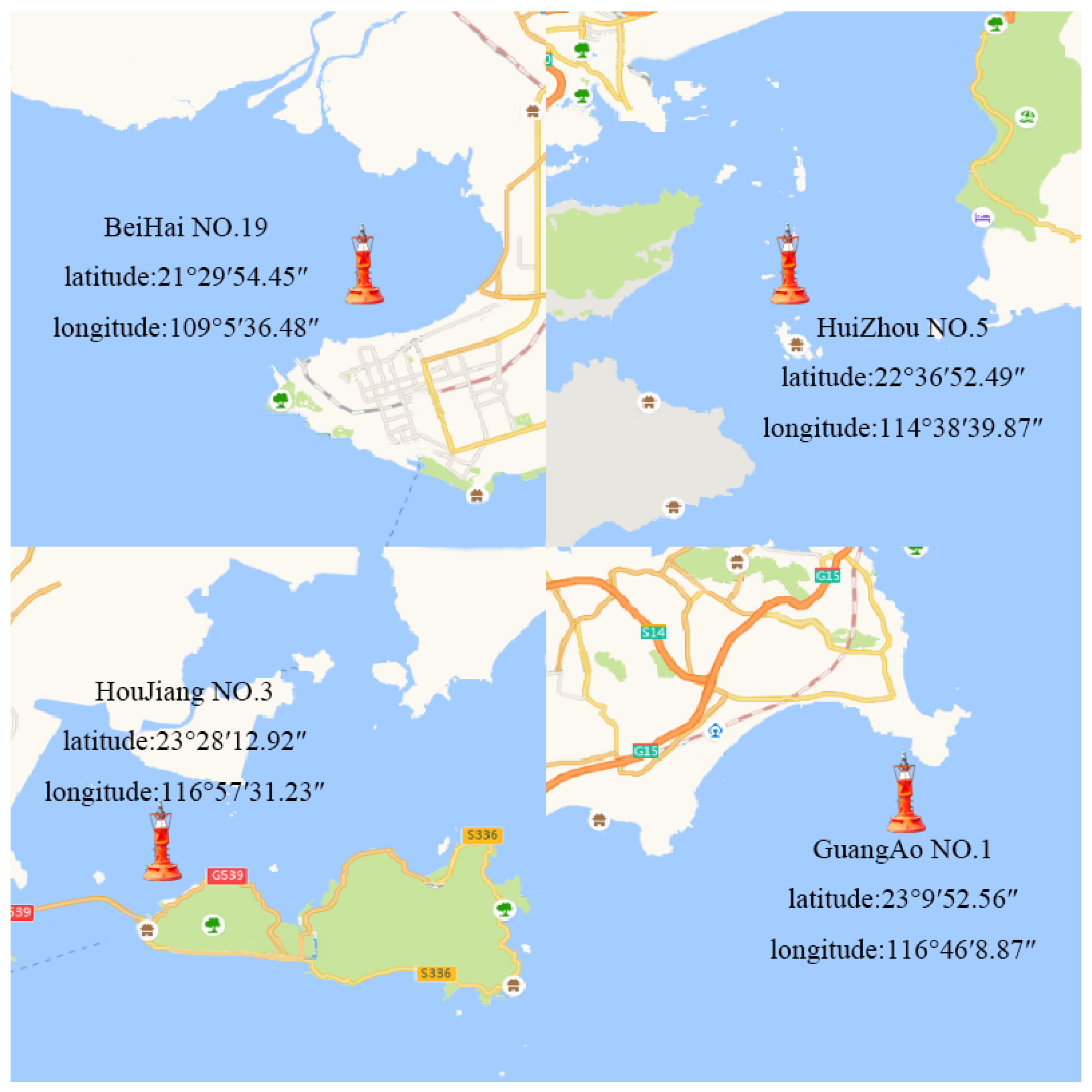
• We conducted a comprehensive comparison of our model with deep learning network models such as LSTM, BiLSTM, 1DCNN, and LSTM-CNN. Through experimental validation on four actual navigation aids datasets collected by the Guangzhou Maritime Safety Administration, the results indicate that our proposed model significantly surpasses current leading methods in terms of performance. This provides strong support for research and practical applications in the field of maritime navigation.

The remaining sections of this research paper are organized as follows: Section 2 provides a detailed exposition of the three feature-processing methods proposed in this paper. Section 3 details the experimental results, and Section 4 summarizes the study and discusses its limitations.

2. Materials and Methods

This chapter provides a detailed introduction to the proposed EFE-LSTM model framework, depicted in Figure 1.

The model consists of three main modules: a feature extension module, a feature fusion module, and a feature extraction module. Firstly, in the feature extension module, the rank entropy operator is introduced, integrating the concept of entropy into the extended space algorithm. This operator effectively captures the uncertainty of data distribution and complex relationships between features, greatly enhancing the model’s ability to handle and understand high-dimensional, complex data. Next, in the feature fusion module, we conduct in-depth feature fusion from three different dimensions: the time domain, frequency domain, and time–frequency domain. The core advantage of this stage lies in the ability to comprehensively consider the relevant characteristics of signals in the time and frequency domains, comprehensively revealing dynamic changes in the navigation state. This multidimensional fusion not only improves the accuracy of recognizing the time patterns and spectral features of navigation signals but also significantly enhances the uniqueness and expressiveness of the model’s features. In the feature extraction module, we employ the BiLSTM model to extract hidden features. The bidirectional modeling capability of the BiLSTM model demonstrates outstanding performance in capturing the spatiotemporal correlations of time series data. Through this step, the model can more accurately grasp the abstract features of navigation signals, thereby effectively distinguishing subtle differences between various navigation aid states. Finally, after finely processing the original features through the three aforementioned modules, the LSTM base model is employed for navigation state recognition.

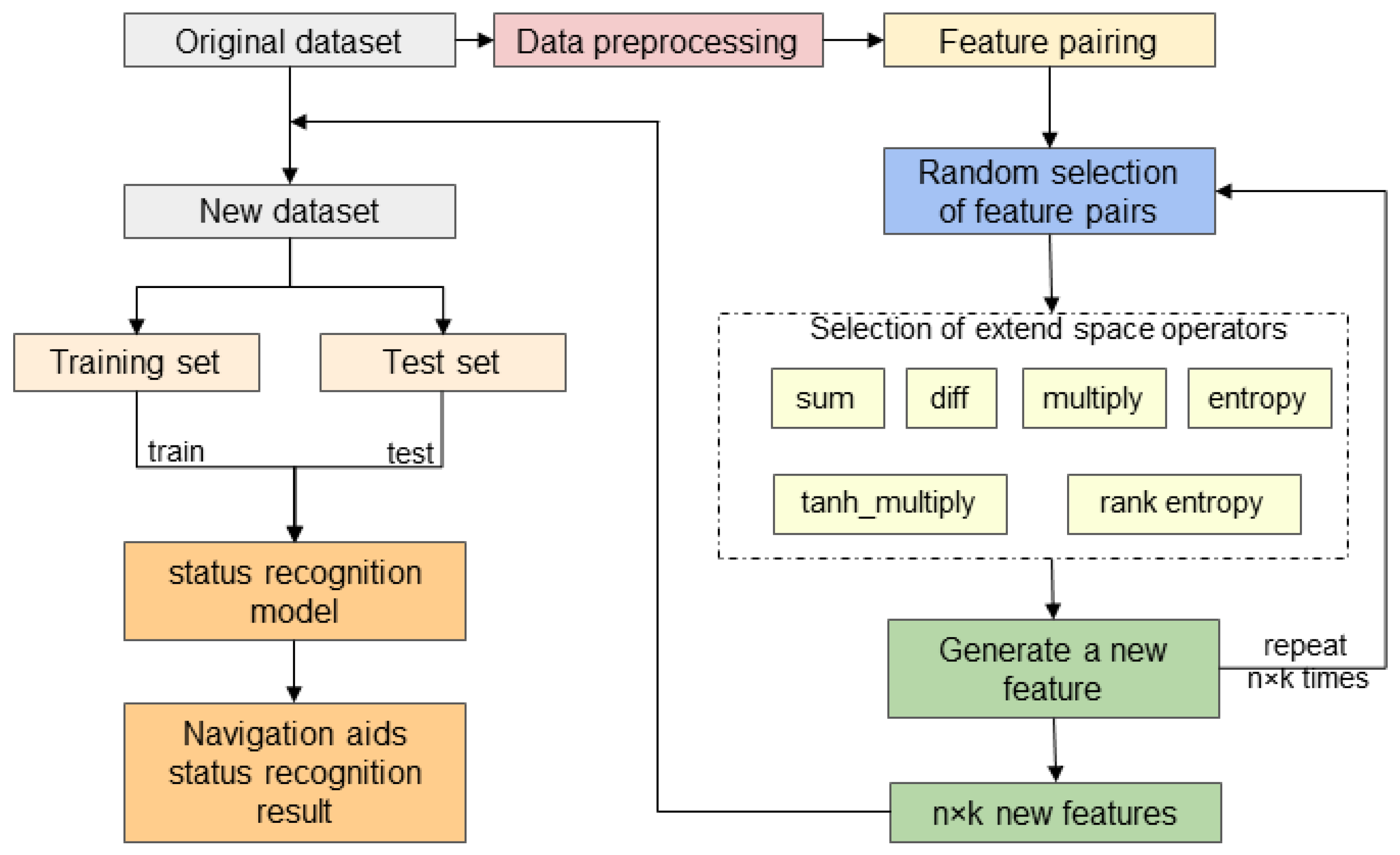
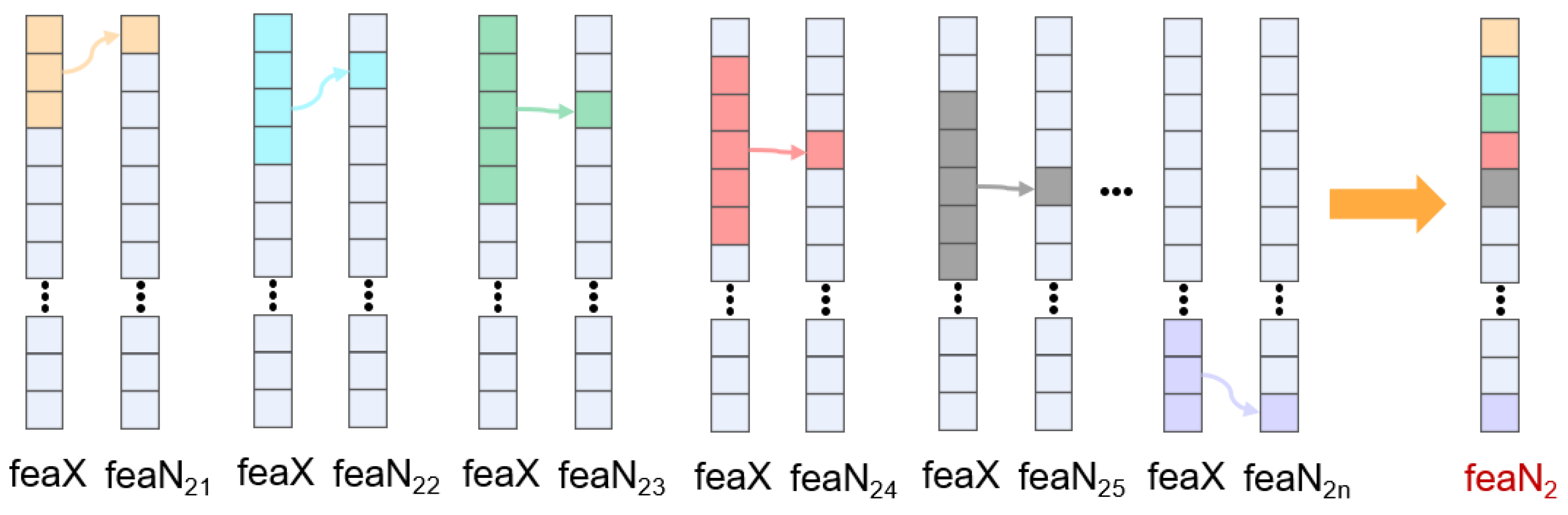
2.1. Feature Extension Module

The Extended Space Forest (ESF) [24] method marks a progressive strategy in building decision trees, incorporating an innovative training tactic that employs both the existing features and those created via random combinations. This approach of feature amalgamation not only broadens the diversity of data portrayal but also elevates data collection quality. The ESF algorithm exhibits exceptional performance in classification predictions, surpassing traditional approaches, particularly in situations with datasets containing a limited number of features.

The core concept of this module rests on the generation of new features through the application of a series of simple yet effective feature-generating operators (such as sum, diff, multiply, and tanh_multiply) on randomly paired sets of original features. The detailed procedure for this method is outlined in

Table 1. Feature-generating operators.

Operator Name	Equation
Sum	$NewFea=feaX+feaY$
Diff	$NewFea=feaX-feaY$
Multiply	$NewFea=feaX\times feaY$
Tanh_multiply	$NewFea=tanh(feaX\times feaY)$

, where feaX and feaY denote any two features from the original dataset. To eliminate bias arising from predetermined feature ordering, the algorithm initially randomizes the arrangement of all features, subsequently selecting pairs from this randomized set for operation to create new features. With n original features, the theoretical maximum number of feature pairs that can be generated is $n\ast (n-1)/2$, which could potentially lead to duplicate features. Consequently, this study opts to generate only $n/2$ new features at a time, and through a process repeated twice, it effectively generates a total of n new features. The process flow of the ESF algorithm is illustrated in Figure 2.

Entropy plays a pivotal role in information theory, in which it serves as a metric for quantifying the uncertainty and information content associated with random variables. Within the domain of state recognition, the field of feature engineering strives to identify features that exhibit enhanced discriminative capabilities across distinct categories. The incorporation of entropy values is primarily geared toward cultivating a profound comprehension of the information interdependencies among features, thereby increasing feature distinctiveness and consequently optimizing model performance.

To begin, we calculate the entropy value for each feature and normalize it to serve as a coefficient for the original feature. This step is designed to introduce information interplay among features, leveraging the entropy value to precisely evaluate each feature’s significance. Features with high entropy, indicative of a wealth of information, are accorded great weight, while features with low entropy, indicating a dearth of information, receive a correspondingly reduced weight. This augmentation significantly bolsters the model’s capacity to acquire data, especially in complex datasets in which the interrelationship between features assumes heightened significance. The process for generating new features is as follows:

$$NewFea=w_1·x_1+w_2·x_2.$$

(1)

Here, $x_1$ and $x_2$ represent any two original features, and $w_1$ and $w_2$ represent the entropy values of the corresponding $x_1$ and $x_2$.

To broaden our analytical scope, we develop a method for determining the relative ranking of each sample’s features and design a new operator named rank entropy. Its fundamental principle unfolds as follows: initially, we employ an exponential function to map each feature value of every sample to the realm of probability, ensuring that data points with lower rankings receive higher probabilities. Specifically, for the ith sample ($i=1,2,3,\dots ,m$), the probability mapping process for the jth ($j=1,2,3,\dots ,n$) feature value can be elucidated through the ensuing equation, where $x_{ij}$ represent the jth feature value of the ith sample., and $r_{ij}$ denotes the rank of $x_{ij}$ within the feature values, ranging from 1 to n. The parameter $\lambda$ is a modifiable factor that regulates the steepness of the probability distribution. Through the computation of Equation (2), we derive the probability distribution $p\left(x_{ij}\right)$ among the features.

$$p\left(x_{ij}\right)=e^{-\lambda ·r_{ij}·x_{ij}}.$$

(2)

Subsequently, we substitute these probability values into Equation (3) to calculate the feature entropy $H\left(x_i\right)$, where $x_i$ denotes the ith sample vector. By calculating the entropy value of each sample for the jth feature, a new feature $fea{N}_1={[H\left(x_1\right),H\left(x_2\right),\dots ,H\left(x_m\right)]}^T$ can be obtained.

$$H\left(x_i\right)=-\sum _{j=1}^{n}p\left(x_{ij}\right)log\left(p\left(x_{ij}\right)\right).$$

(3)

In comparison to traditional extended space operators such as sum, diff, etc., this operator enables us to calculate the rank entropy value between any two features. This rank entropy value can be perceived as a new feature, serving to more accurately capture the interrelations between features, thereby enhancing model performance and the precision of data analysis.

2.2. Feature Fusion Module

This module focuses on introducing the time domain, frequency domain, and time–frequency domain features adopted in this study, along with their corresponding computational formulas.

(1)

Time domain features: The temporal features employed in this study include the following: the mean value $F_{t1}$, variance $F_{t2}$, mean square value $F_{t3}$, root mean square value $F_{t4}$, maximum value $F_{t5}$, minimum value $F_{t6}$, peak value $F_{t7}$, peak-to-peak value $F_{t8}$, and root amplitude $F_{t9}$. Additionally, dimensionless indicators include skewness $F_{t10}$, kurtosis $F_{t11}$, a waveform indicator $F_{t12}$, a peak indicator $F_{t13}$, an impulse indicator $F_{t14}$, a clearance indicator $F_{t15}$, a skewness indicator $F_{t16}$, and a kurtosis indicator $F_{t17}$ [30].

(2)

Frequency domain features: The frequency domain describes the relationship between the frequency and amplitude of a signal, usually with frequency as the independent variable and amplitude as the dependent variable. By employing a Fourier transform, the time-domain signal is mapped to the frequency domain. Subsequently, based on the frequency distribution characteristics and trends of the signal, the navigation state or fault conditions of the beacon can be determined. Frequency domain analyses include methods such as spectrum analysis, energy spectrum analysis, and envelope analysis. A basic introduction to these methods is provided below.

(1)

Spectral analysis: A spectrum analysis usually provides more intuitive feature information than time-domain waveforms. For a time-domain signal $x\left(t\right)$, its spectrum $X\left(f\right)$ can be obtained through the Fourier transform:

$$X\left(f\right)={\int }_{-\infty }^{\infty }x\left(t\right)e^{-j2\pi ft}dt.$$

(4)

Here, $X\left(f\right)$ is the frequency domain representation, f is the frequency, and $x\left(t\right)$ is the original time-domain signal.

(2)

Energy spectral analysis: The energy spectrum is the magnitude squared of the signal’s Fourier transform, representing the distribution of energy across different frequencies. The energy spectrum $E\left(f\right)$ of a signal $x\left(t\right)$ can be expressed as follows:

$$E\left(f\right)={\left|X\left(f\right)\right|}^2.$$

(5)

where $\left|X\right(f\left)\right|$ is the magnitude of the Fourier transform $X\left(f\right)$ of the signal $x\left(t\right)$.

(3)

Envelope analysis: An envelope analysis extracts low-frequency signals from high-frequency signals. From a time-domain perspective, it is equivalent to extracting the envelope trajectory of a time-domain waveform. First, the analytic signal $x_a\left(t\right)$ of the signal $x\left(t\right)$ can be obtained via the Hilbert transform:

$$x_a\left(t\right)=x\left(t\right)+j\widehat{x}\left(t\right).$$

(6)

where $\widehat{x}\left(t\right)$ is the Hilbert transform of $x\left(t\right)$. The envelope $E\left(t\right)$ can then be determined by calculating the magnitude of the analytic signal:

$$E\left(t\right)=|x_a\left(t\right)|=\sqrt{x{\left(t\right)}^2+\widehat{x}{\left(t\right)}^2}.$$

(7)

(3)

Time–frequency domain features: Time–frequency analysis methods provide a more comprehensive description of the relationship between frequency, energy, and time for non-stationary signals. Classical methods for analyzing non-stationary signals include the short-time Fourier transform (STFT) [31] and wavelet decomposition [32], both of which serve as important tools in the analysis of non-stationary signals. These methods can effectively illustrate variations in the frequency and energy of a signal at different time points. The STFT is suited for signals whose frequency content changes gradually over time, whereas wavelet decomposition is more appropriate for signals with sharp transitions or localized features.

(1)

Short-time Fourier transform: The STFT operates by sliding a window across the signal and performing a Fourier transform on the signal within this window. This approach reveals the frequency content of the signal at various time instances. The formula for STFT is expressed as follows:

$$STFT\left\{x\left(t\right)\right\}(\tau ,\omega )=\int x\left(t\right)w(t-\tau )e^{-j\omega t}dt.$$

(8)

Here, $x\left(t\right)$ represents the original signal, $w(t-\tau )$ denotes the window function centered at $\tau$, and $\omega$ is the frequency variable.

(2)

Wavelet decomposition: Wavelet decomposition involves analyzing the signal using a series of wavelet functions derived by scaling and translating a mother wavelet. This method provides insights into the signal’s characteristics at different scales (frequencies) and locations (times). The wavelet decomposition is formulated as follows:

$$W_x(a,b)=\int x\left(t\right)\frac{1}{\sqrt{a}}\psi \left(\frac{t-b}{a}\right)dt.$$

(9)

In this equation, $x\left(t\right)$ is the original signal, $\psi \left(t\right)$ is the mother wavelet function, a is the scaling parameter, and b is the translation parameter.

Multi-domain feature fusion is a data-processing process aimed at enhancing the feature representation of time series datasets. The key steps of this process are as follows:

(a)

For each feature column, we employ a time window with a length of n to slide over each sampling data point, including the current sampling point and its adjacent two sampling points.

(b)

Calculate specific time domain or frequency domain features, such as the standard deviation, spectral analysis short-time Fourier transform, etc.

(c)

Finally, add the calculated new features to the original feature columns to extend the feature set.

This process enables us to capture local features of time series data while integrating time domain, frequency domain, and time–frequency domain information, thereby improving the diversity and information density of data features. The process of multi-domain feature fusion is depicted in Figure 3.

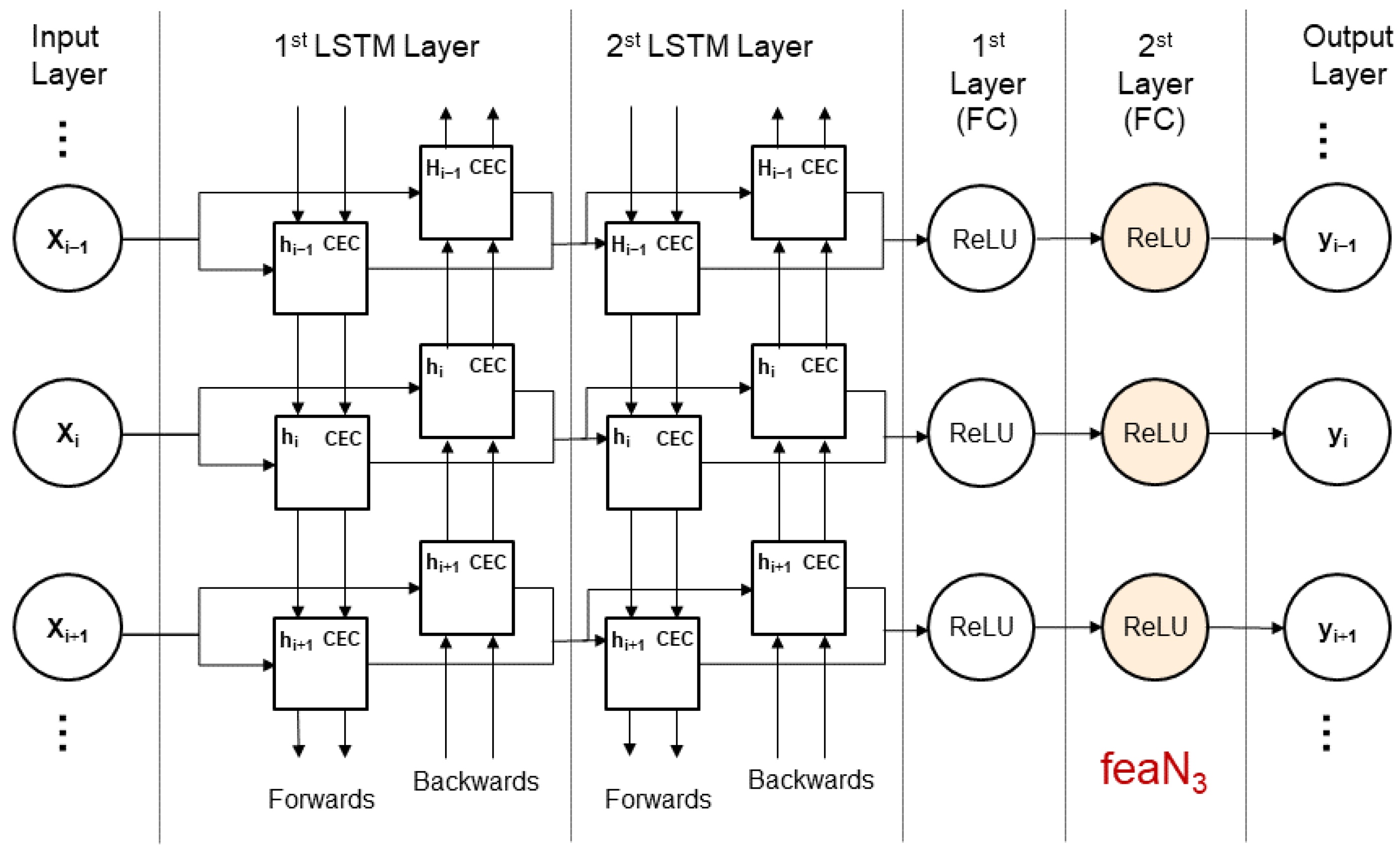
2.3. Feature Extraction Module

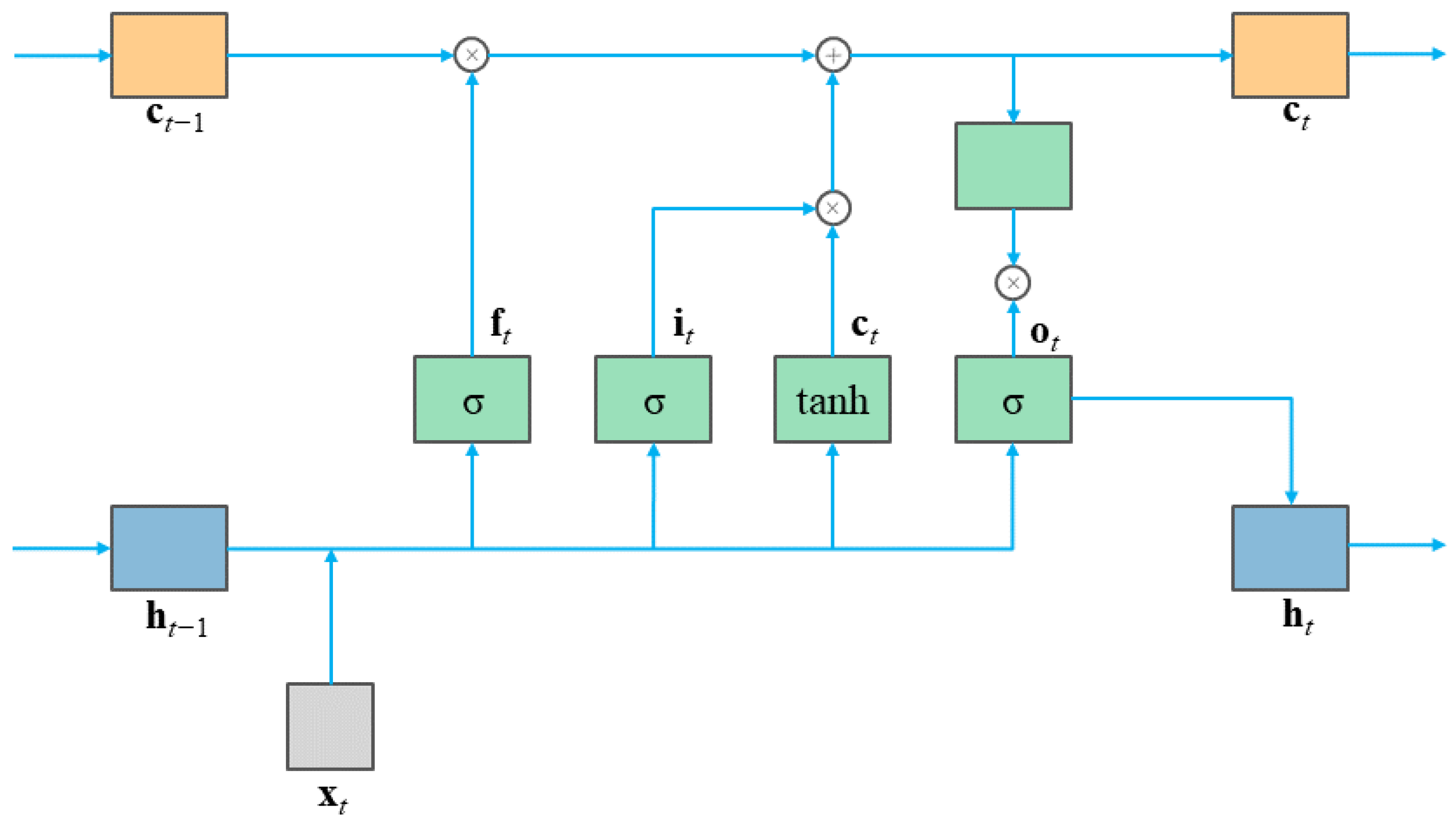
This paper constructs a BiLSTM architecture, as depicted in Figure 4. Utilizing it as a feature converter, the input navigation data are mapped to a new feature space to more effectively express the temporal dependencies within the data. The network comprises an input layer, two LSTM layers, two fully connected layers (FCs), and an output layer.

The input layer is responsible for receiving input sequences $X_{i-1},X_i,X_{i+1},\dots$ in which each X represents a different time step of the input feature vector. The first LSTM layer processes the input sequence in the forward direction, with each unit containing a Constant Error Carousel (CEC) for storing and forgetting information as the memory component and a hidden state h representing the network’s short-term memory. The second LSTM layer, similar to the first, processes the sequence in the reverse direction, enabling the network to utilize information from future time steps during training [33]. The subsequent two fully connected layers (FCs) are dense layers, with each neuron connected to all neurons in the preceding layer, facilitating the nonlinear transformation of learned features. The ReLU activation function applied after each FC layer introduces nonlinearity, assisting the network in learning complex data patterns. The output layer provides the final outputs $Y_{i-1},Y_i,Y_{i+1},\dots$, corresponding to the predictions of the input sequence after being processed by the network.

Finally, the hidden features extracted from the first fully connected layer are labeled as $fea{N}_3$. The deep temporal features learned by the BiLSTM reveal critical information about the navigation state, such as variations, periodicities, or anomalous behaviors in the navigation signals, which are not directly evident in the original features. Combining these hidden features with the original features provides a rich feature set for classifier training, enhancing the model’s recognition accuracy and robustness.

2.4. LSTM

The long short-term memory (LSTM) neural network, a specialized variant of recurrent neural networks, demonstrates outstanding performance in sequence modeling and processing, rendering it a crucial algorithm in the realm of deep learning. In recent years, significant progress has been made in LSTM research, particularly in the domain of state recognition [34,35,36,37]. Conventional recurrent neural networks are plagued by issues such as gradient vanishing and exploding, rendering them unsuitable for effective long-sequence modeling. In contrast, LSTM networks incorporate temporal memory units, enabling the adept assimilation of dependencies across varying temporal scales within time series data. Consequently, LSTM exhibits notable efficacy in handling and forecasting events characterized by intervals and delays in time series data. Within the LSTM hidden layer, the computational process of an individual neuron encompasses updating cell states and calculating output values. Internally, each neuron is equipped with three gating functions: the forget gate, input gate, and output gate. These gating functions judiciously regulate input values, memory states, and output values. The structural configuration of a neuron is delineated in Figure 5, with the mathematical formulations for the forget gate, input gate, and output gate denoted, respectively.

$$f_t=\sigma \left(W_f{h}_{t-1}+W_f{x}_t+b_f\right).$$

(10)

$$i_t=\sigma \left(W_i{h}_{t-1}+W_i{x}_t+b_i\right).$$

(11)

$$o_t=\sigma \left(W_o{h}_{t-1}+W_o{x}_t+b_o\right).$$

(12)

In these equations, $h_{t-1}$ represents the hidden state from the previous time step, and $sigma$ denotes the sigmoid function. $f_t$, $i_t$, and $o_t$ denote the computed results of the forget gate, input gate, and output gate states, respectively. $W_f$, $W_i$, and $W_o$ are the weight matrices corresponding to the forget gate, input gate, and output gate, respectively. $b_f$, $b_i$, and $b_o$ represent the bias terms associated with the forget gate, input gate, and output gate. The final output of the LSTM is jointly determined by the output gate and the cell state.

${\tilde{C}}_t$ represents the candidate value vector, and the product of the input value and the candidate value vector is utilized to update the cell state. The computational process is delineated as follows. Here, $W_c$ represents the weight matrix of the input unit state, $b_c$ is the bias term associated with the input unit state, and $tanh$ denotes the activation function. The forget gate regulates the extent to which information is discarded from the current cell state. $o_t$ represents the output value of the neuron, and $h_t$ signifies the hidden state at the current time step.

$${\tilde{C}}_t=tanh\left(W_c{h}_{t-1}+W_c{x}_t+b_c\right).$$

(13)

$$C_t=f_t{C}_{t-1}+i{\tilde{C}}_t.$$

(14)

$$h_t=o_{t}tanh\left(C_t\right).$$

(15)

$$f\left(x\right)=\frac{1}{1+e^{-x}}.$$

(16)

$$f\left(x\right)=tanh\left(x\right).$$

(17)

2.5. Hyperparameter Optimization

The Adam optimizer was utilized in this study to minimize the cross-entropy loss function, with a learning rate set to 0.001. To alleviate overfitting and expedite model convergence, dropout and batch normalization techniques were applied [38,39,40]. The dropout rate was set to 0.3, and the batch size was set to 100. Detailed architecture specifications of the LSTM model can be found in

Table 2. LSTM model summary.

Layer (Type)	Output Shape	Param
lstm_1 (LSTM)	(None, 256)	268,288
dense_3 (Dense))	(None, 256)	65,792
activation_3 (Activation)	(None, 256)	0
dropout_2 (Dropout)	(None, 256)	0
batch_normalization_2 (Batch Normalization)	(None, 256)	1024
dense_4 (Dense)	(None, 64)	16,448
activation_4 (Activation)	(None, 64)	0
dropout_3 (Dropout)	(None, 64)	0
batch_normalization_3 (Batch Normalization)	(None, 64)	256
dense_5 (Dense)	(None, 2)	130
activation_5 (Activation)	(None, 2)	0

.

3. Data Source Description and Analysis of Results

This section aims to validate the effectiveness of the algorithm proposed in this paper through comprehensive experiments. Firstly, we conducted an experimental analysis using four different datasets from the Guangzhou Maritime Bureau. We comprehensively compared and evaluated the navigation aid state recognition results of our proposed EFE-LSTM algorithm combined with a classic LSTM algorithm [41] and an LSTM model with three modules. Subsequently, to verify the stability and reliability of the experimental results, we compared our EFE-LSTM algorithm with other algorithms such as BiLSTM, 1DCNN and LSTM_CNN. To mitigate the impact of random factors on the experimental results, we conducted five repetitions of the experiments and recorded the average results.

3.1. Data Description and Preprocessing

Ensuring diversity in datasets is crucial when evaluating the performance of the navigation aid state recognition model. The data employed in this study originate from the historical records of four navigation buoys managed by the Guangzhou Maritime Bureau. It’s pertinent to note that within the context of this study, the term “navigation aids” refers explicitly to buoys. These datasets encompass various features of the buoys, including longitude, latitude, voltage, current, and offset distance. Specifically, Figure 6 illustrates the geographical coordinates of the four buoys, namely, Beihai Port Buoy No. 19 (Beihai No. 19), Huizhou Port Buoy No. 5 (Huizhou No. 5), Houjiang Waterway Buoy No. 3 (Houjiang No. 3), and Guang’ao Port Area Buoy No. 1 (Guang’ao No. 1), with coordinates as follows: 109°5′36.48″ N, 21°29′54.45″ E; 114°38′39.87″ N, 22°36′52.49″ E; 116°57′31.23″ N, 23°28′12.92″ E; and 116°46′8.87″ N, 23°9′52.56″ E. A detailed description of each dataset is provided in

Table 3. The description of each dataset.

Dataset ID	Dataset Name	Sample Quantity	Feature Quantity
1	Beihai No. 19	26,727	5
2	Huizhou No. 5	5152	5
3	Houjiang No. 3	4891	5
4	Guang’ao No. 1	17,016	5

. The diversity and richness of these datasets hold significant implications for assessing the performance of the navigation buoy state recognition model.

In order to guarantee the model’s robustness and accuracy, this paper employs a range of meticulous data preprocessing techniques. Using historical record table data for Beihai No. 19 as a case study, the dataset spans from 9 September 2019 to 11 July 2023. A portion of the data is displayed in

Table 4. Partial data of Yangjiang Port navigation aid dataset.

Acquisition Time	Latitude	Longitude	Voltage	Current	Offset Distance
9 September 2019 15:04:36	21.48142333	109.08951500	12.3	0	9.7579337793
9 September 2019 15:30:43	21.48151500	109.47328333	12.3	0	8.4548264142
9 September 2019 17:30:46	21.48174833	109.08964500	12.3	0	10.062118750
…	…	…	…	…	…
11 July 2023 13:38:13	21.49850000	109.09360500	13.700	0	13.305813355
11 July 2023 13:48:59	21.49850000	109.09360500	13.700	0.35	9.8824060802
11 July 2023 14:00:47	21.49850500	109.09360500	13.700	0.36	9.6478582663

.

Firstly, we conducted rigorous data cleaning to eliminate samples with abnormal values or errors, which is crucial for reducing interference factors in the dataset. Secondly, when dealing with missing data, this paper adopted a mean imputation strategy to maintain data integrity and availability as much as possible. Next, to enhance the stability of model training and accelerate the convergence speed, we normalized the dataset. This step involved mapping different feature data into a standardized numerical range, effectively reducing biases caused by varying feature scales during the model training process. The normalization formula is presented below:

$$x^{\prime }=\frac{x-x_{min}}{x_{max}-x_{min}}$$

(18)

Here, x represents the original data, $x^{\prime }$ represents the normalized data, and $x_{min}$ and $x_{max}$ represent the minimum and maximum values within the feature vector, respectively.

3.2. Model Evaluation Metrics

When it comes to identifying the state of a navigation aid, there is a significant imbalance in sample categories. If we only use accuracy as the sole evaluation criterion, models that tend to classify unknown samples as majority classes (normal labels) will be considered to have better performance. To avoid this issue, we chose to use several other evaluation criteria, including accuracy, precision, recall, and F1 score, when measuring the performance of the model. The F1 score is a calculation definition that takes into account both precision and recall, providing us with a more comprehensive measure of the model’s performance [42].

$$Accuracy=\frac{TP+TN}{TP+FP+TN+FN}$$

(19)

$$Precision=\frac{TP}{TP+FP}$$

(20)

$$Recall=\frac{TP}{TP+FN}$$

(21)

$$F1=2\times \frac{Precision\times Recall}{Precision+Recall}$$

(22)

3.3. Assessment Results

3.3.1. Experimental Comparison of Extended Space Operators

In a paper by Amasyali, M.F. et al. [24], the concept of extended space was introduced for the first time. However, although traditional extension methods provided a larger feature space for data, they failed to fully exploit the information within the original features. To address this issue, our research innovatively introduces the concept of entropy and proposes a novel rank entropy for feature extraction. This rank entropy not only considers the distribution characteristics of the data but also comprehensively captures the complexity and uncertainty of features within the framework of information theory. The experimental results, as presented in

Table 5. Comparison of performance among different extended space operators.

Operator	Mean Accuracy	Mean Recall	Mean Precision	Mean F1
/	60.53%	74.87%	60.53%	53.59%
Sum	61.03%	71.86%	61.02%	55.39%
Diff	63.10%	74.44%	63.09%	58.22%
Multiply	62.65%	74.10%	62.65%	57.59%
Tanh_multiply	62.99%	73.89%	62.97%	58.31%
Entropy	62.06%	73.31%	62.05%	56.80%
Rank entropy (Proposed)	71.63%	78.66%	71.62%	69.68%

Note: Bold numbers represent the best performance among each evaluation metric. Underlined numbers indicate the second-best performance.

, validate the effectiveness and superiority of our method in feature extraction.

In Table 5, “/” denotes direct model training using the original dataset, while “sum”, “diff”, “multiply”, and “tanh_multiply” represent traditional extended space operators; “entropy” signifies the direct introduction of entropy as a coefficient, and “rank entropy” is the ranking entropy proposed in this paper. All results in the table represent outcomes averaged across the four datasets. The optimal results are highlighted in bold, while the second-best results are underscored.

As illustrated in Table 5, upon the introduction of the extended space operators, an overall improvement in the model’s performance was observed. Among the traditional extended space operators, the “diff” operator exhibited the best performance across four evaluation metrics. Specifically, compared to the direct use of the original dataset, the “diff” operator significantly improved both the average accuracy and average precision by 2.57% and 2.56%, respectively. In terms of the average F1 score, the improvement reached 4.63% when using the “diff” operator compared to the original features. Despite a slight decrease of 0.43% in the average recall rate, considering all four metrics together, the use of the “diff” operator for extended space still shows significant advantages. This indicates that traditional extended space operators effectively enhance the overall performance of the model while maintaining balance.

Furthermore, the direct introduction of the concept of entropy does not lead to a significant performance improvement. Although the “entropy” operator exhibits improvements across all metrics compared to the original model, the improvement is relatively modest. In this context, the proposed “rank entropy” operator stands out. Compared to the traditional extended space operator “diff”, “rank entropy” achieves a significant enhancement in all evaluation metrics. Specifically, relative to “diff”, “rank entropy” improves the average accuracy, recall, precision, and F1 score by approximately 8.53%, 4.22%, 8.53%, and 11.46%, respectively. This indicates that the “rank entropy” operator successfully introduces a more effective feature extraction mechanism, significantly improving the model’s ability to identify navigation aid states. All subsequent experiments in the following text are based on the proposed “rank entropy” operator introduced in this paper.

3.3.2. Select Multi-Domain Features

Through the multi-domain feature fusion method proposed in this paper, the original dataset’s 5 features were extended to 260. An analysis of the features revealed inconsistent correlations between different features and relatively high similarity among some feature values. A PCA was employed for dimensionality reduction, allowing for the elimination of insignificant principal components while retaining maximal data variance. According to the analysis results, the cumulative variance of the first 30 principal components reached 90%, with the remaining components contributing insignificantly to the total variance. Consequently, analyzing these principal components is sufficient for achieving a dimensionality reduction, ensuring the preservation of essential data information. The specific retention states of feature vectors are delineated in

Table 6. Preserved features.

Domain	Reserved Features
Time domain	root amplitude variance skewness indicator kurtosis indicator
Frequency domain	spectral analysis
Time–frequency domain	wavelet decomposition

. Following the PCA-based dimensionality reduction, the overall relationships within the dataset are preserved, critical data information is retained, and a substantial reduction in computational load is achieved during the feature extraction process.

3.3.3. Comparison with Other Feature Extraction Models

In this study, we designed and compared multiple deep-learning models to extract effective hidden features from navigation aid state data. Specifically, we developed four different model architectures: the LSTM model [43], BiLSTM model [44], 1DCNN model [45], and LSTM-CNN model [46], each comprising two respective feature extraction layers and two fully connected layers. All models use the output of the first fully connected layer as the extracted hidden features. The “/” in

Table 7. Comparison with other feature extraction models.

Model	Mean Accuracy	Mean Recall	Mean Precision	Mean F1
/	60.53%	74.87%	60.53%	53.59%
LSTM	62.60%	73.45%	62.60%	57.02%
1DCNN	66.86%	74.48%	66.87%	63.15%
LSTM_CNN	67.10%	73.87%	67.11%	63.97%
BiLSTM	68.35%	74.85%	68.35%	65.51%

Note: Bold numbers represent the best performance among each evaluation metric.

represents direct utilization of raw features without extraction.

As is evident from Table 7, BiLSTM demonstrates significant advantages over other models in multiple key performance indicators. Specifically, BiLSTM achieves an accuracy of 68.35% and an F1 score of 65.51%, reflecting its outstanding performance in overall prediction accuracy and true positive identification. Moreover, BiLSTM exhibits impressive performance in recall and precision, reaching 74.85% and 68.35%, respectively, highlighting its efficient performance in true positive identification and prediction accuracy. These data unequivocally indicate the exceptional performance of BiLSTM in the complex task of extracting features from time-series data.

3.3.4. Comparison of Performance among Different Modules

Next, a detailed comparative analysis of the performance of the standard LSTM, rank entropy LSTM (RE-LSTM), multi-domain feature fusion LSTM (MD-LSTM), and hidden feature extraction LSTM (HF-LSTM) models and the LSTM model incorporating rank entropy extension, multi-domain feature fusion, and hidden feature extraction (EFE-LSTM) was conducted across various datasets, as shown in Figure 7.

Firstly, the introduction of rank entropy results in increases in accuracy for LSTM on the BeiHai and GuangAo datasets by approximately 0.13 and 0.07, respectively, compared to the standard LSTM. This highlights its effectiveness in capturing the importance of sequence elements, emphasizing its crucial role in enhancing the model’s understanding of inherent relationships within the data. Secondly, introducing the multi-domain feature fusion module provides a noticeable improvement in model performance. On the BeiHai, HuiZhou, and GuangAo datasets, TF-LSTM shows an accuracy increase of approximately 0.4 to 0.5 relative to the standard LSTM. This suggests that by fusing multi-domain features, the model can more comprehensively capture changes in the temporal dimension, enhancing its adaptability in the context of complex and variable data backgrounds. Thirdly, the introduction of the hidden feature extraction module leads to a slight increase in accuracy for LSTM on the BeiHai and GuangAo datasets relative to the standard LSTM, with an improvement of about 0.2 to 0.3. On the HuiZhou dataset, the improvement for HF-LSTM is more pronounced at around 0.2. This demonstrates that the hidden feature extraction module has a significant positive effect on capturing abstract features within the data.

Finally, the EFE-LSTM model, integrating the rank entropy, multi-domain feature fusion, and hidden feature extraction modules, demonstrates outstanding performance across all datasets. The EFE-LSTM model achieves an accuracy increase of approximately 0.4 on the BeiHai dataset relative to the standard LSTM, while the improvements on the HuiZhou and GuangAo datasets are more significant, ranging from 0.4 to 0.5. This further validates that by integrating different feature fusion modules, our model can more comprehensively and accurately capture key features in multidimensional time data. This provides an effective and comprehensive modeling approach for multidimensional time data classification tasks, as demonstrated by experimental validation. Even without relying on a complex network structure, the proposed method achieves highly accurate navigation state recognition, highlighting the robust performance and practical value of this approach.

3.3.5. Comparison of Performance among Different Models

Finally, this paper provides a comprehensive comparison of different models in the navigation aid state recognition task, as depicted in

Table 8. Performance metrics for different methods on four datasets.

Beihai No. 19
Method	Confusion Matrix		Mean Accuracy	Mean Precision	Mean Recall	Mean F1
LSTM	961.8	48.4	0.6511	0.7505	0.6507	0.6134
	656.6	353.6
BiLSTM	907.8	102.4	0.6602	0.7124	0.6606	0.6352
	584.2	426
1DCNN	947.2	63	0.7821	0.8125	0.7821	0.7767
	377.2	633
LSTM-CNN	971.8	38.4	0.7614	0.8119	0.7614	0.7514
	443.6	566.6
EFE-LSTM	1004.2	6	0.9922	0.9921	0.9922	0.9922
	9.8	1000.4
Huizhou No. 5
Method	Confusion Matrix		Mean Accuracy	Mean Precision	Mean Recall	Mean F1
LSTM	185	14	0.7010	0.7547	0.7008	0.6841
	105	94
BiLSTM	164.8	34.2	0.7020	0.7173	0.7022	0.6969
	84.4	114.6
1DCNN	180.6	18.4	0.7231	0.7584	0.7233	0.7133
	91.8	107.2
LSTM-CNN	181.2	17.8	0.7085	0.7497	0.7087	0.6959
	98.2	100.8
EFE-LSTM	189.4	9.6	0.9191	0.9212	0.9191	0.9189
	22.6	176.4
Houjiang No. 3
Method	Confusion Matrix		Mean Accuracy	Mean Precision	Mean Recall	Mean F1
LSTM	175.4	8.8	0.5994	0.7013	0.5996	0.5418
	138.8	45.4
BiLSTM	177.2	7	0.5874	0.7001	0.5875	0.5199
	145	39.2
1DCNN	173.6	10.6	0.5993	0.6890	0.5995	0.5456
	137	47.2
LSTM-CNN	171.6	12.6	0.5988	0.6788	0.5995	0.5456
	135.2	49
EFE-LSTM	166	18.2	0.8334	0.8404	0.8339	0.8325
	43.2	141
Method	Confusion Matrix		Mean Accuracy	Mean Precision	Mean Recall	Mean F1
LSTM	598.4	21.2	0.5734	0.6913	0.5734	0.4956
	507.4	112.2
BiLSTM	584.2	35.4	0.5689	0.6636	0.5699	0.4978
	498.8	120.8
1DCNN	577.6	42	0.6067	0.6876	0.6074	0.5599
	445.4	174.2
LSTM-CNN	598.2	21.4	0.5778	0.6947	0.5778	0.5030
	501.8	117.8
EFE-LSTM	588.4	31.2	0.9385	0.9387	0.9387	0.9385
	45	574.6

Note: The gray background in the confusion matrix cells highlights true positives and true negatives.

. Compared to 1DCNN, EFE-LSTM demonstrates more stable and significant improvements in accuracy. Across various datasets, EFE-LSTM’s accuracy increases by approximately 0.12 to 0.28 relative to 1DCNN. In comparison to LSTM-CNN, EFE-LSTM exhibits a more noticeable improvement in accuracy. Across multiple datasets, EFE-LSTM’s accuracy increases by about 0.05 to 0.16 compared to LSTM-CNN. When compared to BiLSTM, EFE-LSTM consistently shows higher accuracy across multiple datasets, with an improvement ranging from 0.28 to 0.41. Relative to TCN, EFE-LSTM also achieves higher accuracy, with an improvement ranging from 0.16 to 0.27.

In summary, EFE-LSTM outperforms models such as 1DCNN, LSTM-CNN, BiLSTM, and TCN in multidimensional time data classification tasks. Its performance improvement is not only remarkable across various datasets but also demonstrates significant advantages in capturing time series information and handling complex associations in comparisons with different models.

4. Conclusions

This paper introduces the EFE-LSTM model, which achieves significant progress in the recognition of navigation beacon states through the integration of entropy space extension, multi-domain feature fusion, and hidden feature extraction. Its primary advantage lies in extending the feature space through rank entropy, allowing for a more nuanced understanding of complex signal patterns by capturing uncertainty in data distribution. Additionally, the model integrates time and frequency domain features, providing a multidimensional and comprehensive representation of the data, which is crucial for accurately capturing the dynamic evolution of navigation beacon states. Finally, extracting hidden features from the data to capture abstract representations of beacon signals further enhances the modeling capability for navigation beacon states. Compared to traditional models, the proposed EFE-LSTM model achieved average accuracy rates of 99.22%, 91.91%, 83.34%, and 93.85% on four datasets, respectively. This represents an improvement of over 20% in accuracy compared to the best-performing model in traditional models for navigational beacon state recognition, highlighting its robustness in handling complex multidimensional temporal data.

Future research should focus on enhancing the real-time performance of the model and further optimizing computational efficiency to ensure that the model maintains excellent performance when processing large datasets. Additionally, exploring a variety of feature extension methods to enhance the model’s generalizability will be an important research direction. Moreover, constructing more complex deep learning models to delve deeper into the intrinsic connections among data could also improve the accuracy of status recognition.

References

1. Redondo, R.; Atienza, R.; Pecharroman, L.; Pires, L. Aids to navigation improvement to optimize ship navigation. In Smart Rivers; Springer: Berlin/Heidelberg, Germany, 2022; pp. 803–813. [Google Scholar]
2. Sang, L.; Hong, S. Development of navigational aids telemetry and telecontrol system in south China sea. Navig. China 2020, 43, 35–40. [Google Scholar]
3. Wen, Z.; Cao, J.; Huang, L.; Li, D.; Sun, L.; Huang, X. Enhancing Navigation Aids Status Recognition Based on Extended Space Forest and Time Domain Features Fusion. In Proceedings of the 2023 IEEE International Symposium on Product Compliance Engineering—Asia (ISPCE-ASIA), Shanghai, China, 3–5 November 2023; pp. 1–6. [Google Scholar]
4. Muhammad Irsyad Hasbullah, N.A.O.; Salleh, N.H.M. A systematic review and meta-analysis on the development of aids to navigation. Aust. J. Marit. Ocean. Aff. 2023, 15, 247–267. [Google Scholar] [CrossRef]
5. Cho, M.; Choi, H.R.; Kwak, C. A study on the navigation aids management based on IoT. Int. J. Control Autom. 2015, 8, 193–204. [Google Scholar] [CrossRef]
6. Cho, M.; Choi, H.; Kwak, C. A Study on the method of IoT-based navigation aids management. Adv. Sci. Technol. Lett. 2015, 98, 55–58. [Google Scholar]
7. Ostroumov, I.; Kuzmenko, N. Risk analysis of positioning by navigational aids. In Proceedings of the 2019 Signal Processing Symposium (SPSympo), Krakow, Poland, 17–19 September 2019; IEEE: Piscataway, NJ, USA, 2019; pp. 92–95. [Google Scholar]
8. Ostroumov, I.; Kuzmenko, N. Risk assessment of mid-air collision based on positioning performance by navigational aids. In Proceedings of the 2020 IEEE 6th International Conference on Methods and Systems of Navigation and Motion Control (MSNMC), Kyiv, Ukraine, 20–23 October 2020; IEEE: Piscataway, NJ, USA, 2020; pp. 34–37. [Google Scholar]
9. Wu, F.; Qu, Y. The positive impact of intelligent aids to navigation on maritime transportation. In Proceedings of the Seventh International Conference on Traffic Engineering and Transportation System (ICTETS 2023), Dalian, China, 22–24 September 2023; SPIE: Washington, DC, USA, 2024; Volume 13064, pp. 959–966. [Google Scholar]
10. Liang, Y. Route planning of aids to navigation inspection based on intelligent unmanned ship. In Proceedings of the 2021 4th International Symposium on Traffic Transportation and Civil Architecture (ISTTCA), Suzhou, China, 12–14 November 2021; IEEE: Piscataway, NJ, USA, 2021; pp. 95–98. [Google Scholar]
11. Alharbi, N.S.; Jahanshahi, H.; Yao, Q.; Bekiros, S.; Moroz, I. Enhanced classification of heartbeat electrocardiogram signals using a long short-term memory–convolutional neural network ensemble: Paving the way for preventive healthcare. Mathematics 2023, 11, 3942. [Google Scholar] [CrossRef]
12. Mustaqeem; Kwon, S. CLSTM: Deep feature-based speech emotion recognition using the hierarchical ConvLSTM network. Mathematics 2020, 8, 2133. [Google Scholar] [CrossRef]
13. Chen, Y.; Niu, G.; Li, Y.; Li, Y. A modified bidirectional long short-term memory neural network for rail vehicle suspension fault detection. Veh. Syst. Dyn. 2023, 61, 3136–3160. [Google Scholar] [CrossRef]
14. Dong, L.; Zhang, H.; Yang, K.; Zhou, D.; Shi, J.; Ma, J. Crowd counting by using Top-k relations: A mixed ground-truth CNN framework. IEEE Trans. Consum. Electron. 2022, 68, 307–316. [Google Scholar] [CrossRef]
15. An, Z.; Li, S.; Wang, J.; Jiang, X. A novel bearing intelligent fault diagnosis framework under time-varying working conditions using recurrent neural network. ISA Trans. 2020, 100, 155–170. [Google Scholar] [CrossRef]
16. Alotaibi, N.D.; Jahanshahi, H.; Yao, Q.; Mou, J.; Bekiros, S. An ensemble of long short-term memory networks with an attention mechanism for upper limb electromyography signal classification. Mathematics 2023, 11, 4004. [Google Scholar] [CrossRef]
17. Wang, H.; Fu, S.; Peng, B.; Wang, N.; Gao, H. Equipment health condition recognition and prediction based on CNN-LSTM deep learning. In Proceedings of the International Conference on Maintenance Engineering, Online, 15–17 April 2020; Springer: Berlin/Heidelberg, Germany, 2020; pp. 830–842. [Google Scholar]
18. Zhao, H.; Hou, C.; Alrobassy, H.; Zeng, X. Recognition of transportation state by smartphone sensors using deep BiLSTM neural network. J. Comput. Netw. Commun. 2019, 2019, 830–842. [Google Scholar]
19. Mekruksavanich, S.; Jitpattanakul, A. Lstm networks using smartphone data for sensor-based human activity recognition in smart homes. Sensors 2021, 21, 1636. [Google Scholar] [CrossRef] [PubMed]
20. Wang, C.; Luo, H.; Zhao, F.; Qin, Y. Combining residual and LSTM recurrent networks for transportation mode detection using multimodal sensors integrated in smartphones. IEEE Trans. Intell. Transp. Syst. 2020, 22, 5473–5485. [Google Scholar] [CrossRef]
21. Wang, H.; Luo, H.; Zhao, F.; Qin, Y.; Zhao, Z.; Chen, Y. Detecting Transportation Modes with Low-Power-Consumption Sensors Using Recurrent Neural Network; IEEE: Piscataway, NJ, USA, 2018; pp. 1098–1105. [Google Scholar]
22. Drosouli, I.; Voulodimos, A.; Miaoulis, G.; Mastorocostas, P.; Ghazanfarpour, D. Transportation mode detection using an optimized long short-term memory model on multimodal sensor data. Entropy 2021, 23, 1457. [Google Scholar] [CrossRef] [PubMed]
23. Shi, L.; Liu, Z.; Zhou, K.; Shi, Y.; Jing, X. Novel deep learning network for gait recognition using multimodal inertial sensors. Sensors 2023, 23, 849. [Google Scholar] [CrossRef] [PubMed]
24. Amasyali, M.F.; Ersoy, O.K. Classifier ensembles with the extended space forest. IEEE Trans. Knowl. Data Eng. 2013, 26, 549–562. [Google Scholar] [CrossRef]
25. Dhibi, K.; Mansouri, M.; Bouzrara, K.; Nounou, H.; Nounou, M. An enhanced ensemble learning-based fault detection and diagnosis for grid-connected PV systems. IEEE Access 2021, 9, 155622–155633. [Google Scholar] [CrossRef]
26. Sun, H.; Zhao, S. Fault diagnosis for bearing based on 1DCNN and LSTM. Shock Vib. 2021, 2021, 1–17. [Google Scholar] [CrossRef]
27. Malik, A.K.; Ganaie, M.; Tanveer, M.; Suganthan, P.N. Extended features based random vector functional link network for classification problem. IEEE Trans. Comput. Soc. Syst. 2022. [Google Scholar] [CrossRef]
28. Xu, Y.; Yu, Z.; Cao, W.; Chen, C.P. A novel classifier ensemble method based on subspace enhancement for high-dimensional data classification. IEEE Trans. Knowl. Data Eng. 2021, 35, 16–30. [Google Scholar] [CrossRef]
29. Wang, Y.; Wang, S.; Sima, X.; Song, Y.; Cui, S.; Wang, D. Expanded feature space-based gradient boosting ensemble learning for risk prediction of type 2 diabetes complications. Appl. Soft Comput. 2023, 144, 110451. [Google Scholar] [CrossRef]
30. Duan, Y.; Cao, X.; Zhao, J.; Xu, X. Health indicator construction and status assessment of rotating machinery by spatiotemporal fusion of multi-domain mixed features. Measurement 2022, 205, 112170. [Google Scholar] [CrossRef]
31. Boashash, B. Time-Frequency Signal Analysis and Processing: A Comprehensive Reference; Academic Press: Cambridge, MA, USA, 2015. [Google Scholar]
32. Mallat, S.G. A theory for multiresolution signal decomposition: The wavelet representation. IEEE Trans. Pattern Anal. Mach. Intell. 1989, 11, 674–693. [Google Scholar] [CrossRef]
33. Abduljabbar, R.L.; Dia, H.; Tsai, P.W. Development and evaluation of bidirectional LSTM freeway traffic forecasting models using simulation data. Sci. Rep. 2021, 11, 23899. [Google Scholar] [CrossRef]
34. Xia, K.; Huang, J.; Wang, H. LSTM-CNN architecture for human activity recognition. IEEE Access 2020, 8, 56855–56866. [Google Scholar] [CrossRef]
35. Khan, P.; Reddy, B.S.K.; Pandey, A.; Kumar, S.; Youssef, M. Differential channel-state-information-based human activity recognition in IoT networks. IEEE Internet Things J. 2020, 7, 11290–11302. [Google Scholar] [CrossRef]
36. Du, X.; Ma, C.; Zhang, G.; Li, J.; Lai, Y.K.; Zhao, G.; Deng, X.; Liu, Y.J.; Wang, H. An efficient LSTM network for emotion recognition from multichannel EEG signals. IEEE Trans. Affect. Comput. 2020, 13, 1528–1540. [Google Scholar] [CrossRef]
37. Xiao, H.; Sotelo, M.A.; Ma, Y.; Cao, B.; Zhou, Y.; Xu, Y.; Wang, R.; Li, Z. An improved LSTM model for behavior recognition of intelligent vehicles. IEEE Access 2020, 8, 101514–101527. [Google Scholar] [CrossRef]
38. Kingma, D.P.; Ba, J. Adam: A method for stochastic optimization. arXiv 2014, arXiv:1412.6980. [Google Scholar]
39. Srivastava, N.; Hinton, G.; Krizhevsky, A.; Sutskever, I.; Salakhutdinov, R. Dropout: A simple way to prevent neural networks from overfitting. J. Mach. Learn. Res. 2014, 15, 1929–1958. [Google Scholar]
40. Ioffe, S.; Szegedy, C. Batch normalization: Accelerating deep network training by reducing internal covariate shift. In Proceedings of the International Conference on Machine Learning, Lille, France, 7–9 July 2015; Volume 37, pp. 448–456. [Google Scholar]
41. Dogan, G.; Ford, M.; James, S. Predicting ocean-wave conditions using buoy data supplied to a hybrid RNN-LSTM neural network and machine learning models. In Proceedings of the 2021 IEEE International Conference on Machine Learning and Applied Network Technologies (ICMLANT), Soyapango, El Salvador, 16–17 December 2021; pp. 1–6. [Google Scholar]
42. Powers, D.M.W. Evaluation: From precision, recall and F-measure to ROC, informedness, markedness and correlation. arXiv 2020, arXiv:2010.16061. [Google Scholar]
43. Sherstinsky, A. Fundamentals of recurrent neural network (RNN) and long short-term memory (LSTM) network. Phys. D Nonlinear Phenom. 2020, 404, 132306. [Google Scholar] [CrossRef]
44. Woźniak, M.; Wieczorek, M.; Siłka, J. BiLSTM deep neural network model for imbalanced medical data of IoT systems. Future Gener. Comput. Syst. 2023, 141, 489–499. [Google Scholar] [CrossRef]
45. Huang, S.; Tang, J.; Dai, J.; Wang, Y. Signal status recognition based on 1DCNN and its feature extraction mechanism analysis. Sensors 2019, 19, 2018. [Google Scholar] [CrossRef]
46. Kim, T.; Kim, H.Y. Forecasting stock prices with a feature fusion LSTM-CNN model using different representations of the same data. PLoS ONE 2019, 14, e0212320. [Google Scholar] [CrossRef]
Figure 1. The framework of the EFE-LSTM model.
Mathematics 12 01048 g001
Figure 2. ESF algorithm flowchart.
Mathematics 12 01048 g002
Figure 3. The process of the feature fusion module.
Mathematics 12 01048 g003
Figure 4. The architectural diagram of the feature extraction network.
Mathematics 12 01048 g004
Figure 5. The hidden layer structure of LSTM.
Mathematics 12 01048 g005
Figure 6. Schematic diagram of the position of the light buoy.
Mathematics 12 01048 g006
Figure 7. Comparison of classification accuracies of five models.
Mathematics 12 01048 g007