Simulation and Optimization of a Dual-Axis Solar Tracking Mechanism

Abstract

The work deals with the simulation and optimization of a tracking mechanism used to increase the efficiency of photovoltaic (PV) systems. The proposed solar tracker is one with two degrees of freedom (so called dual-axis, or bi-axial), of the equatorial/polar type. The actuation of the tracking system is carried out with two linear actuators, one for each of the two movements. The study is carried out using a virtual prototyping platform that integrates, into a mechatronic concept, the commercial software packages ADAMS and EASY5. The optimization process is approached from three points of view, which target the mechanical device, the control system, and the bi-axial tracking program. All these optimization processes positively influence, in a specific way, the energy efficiency of the tracking system, which was comprehensively evaluated considering the data specific to the longest light-day of the year (i.e., summer solstice), where a net energy gain of 58.66% (by reference to the equivalent fixed system) was obtained. Similar numerical simulations corresponding to several representative days of the year have revealed that the annual net energy gain is around 42%, which fully justifies the use of the proposed tracking system.

1. Introduction

We all know the problems involved in the use of fossil fuels, in addition to their limited nature, such as global warming, the greenhouse effect, and pollution. All of these generate effects that we already see in the major climate changes that humanity is facing and which may evolve dramatically in the future. The well-known American inventor, engineer, and businessman Charles Franklin Kettering said, “We should all be concerned about the future because we will have to spend the rest of our lives there”. Research in the field of renewable energy systems (RESs) is a worldwide priority, because these green power “plants” can provide long-term environmentally friendly solutions. The Sun is the most important source of renewable energy, either directly or indirectly, and the current technology allows for the conversion of solar radiation into thermal or electrical energy. There are two solutions for producing electric power from the Sun, Concentrated Solar Power (CSP) and photovoltaic (PV) systems [1,2,3], the latter being addressed in this work.

Improving the efficiency of PV systems is a continuing concern and challenge for contemporary research, with two methods being frequently approached in this regard: (I) improving the conversion yield at the level of the PV module, which mainly involves the use of more efficient materials, and (II) increasing the degree of capture of solar radiation, which is achieved through the optimal positioning of the PV module depending on the sun’s position on the celestial vault during daylight, by using so-called solar tracking systems (solar trackers). Paraphrasing an old Maori proverb, “Turn your face to the sun and the shadows fall behind you”, the subject of this work can be rendered in the following form: turn the PV module to the sun and the shadows fall behind it. By adding solar trackers to the PV systems, their energy efficiency can increase in a fairly wide and diverse range of values (20–60%) relative to the equivalent fixed (stationary) system, according to the type of tracking mechanism (its number of degrees of freedom), the control strategy, and the specific location (including climatic conditions). With the purpose of exemplifying this, several data examples from the literature are presented in

Table 1. Energy gain for several PV tracking mechanisms.

References	Tracking System Type	Control Strategy	Location (Latitude/Longitude)	Energy Gain
[4]	dual-axis	open-loop	45.657974 N/25.601198 E	41.45%
[5]	dual-axis	closed-loop	12.873498 N/80.219866 E	27%
[6]	dual-axis	open-loop	33.838 N/−6.083 W	35.71%
[7]	dual-axis	close-loop	29.571858 N/57.301047 E	31.8%
[8]	single-axis	open-loop	−29.72404 S/−53.71081 W	25.76%
[9]	single-axis	open-loop	25.037519 N/121.563679 E	24.2%
[10]	dual-axis	closed-loop	12.824342 N/101.216274 E	44.89%
[11]	dual-axis	open-loop	45.657974 N/25.601198 E	29.6%
[12]	single|dual-axis	closed-loop	26.43442 N/50.10326 E	18.73%|28.98%
[13]	single|dual-axis	closed-loop	13.072090 N/80.201859 E	20%|40%
[14]	dual-axis	open-loop	−29.68605 S/−53.80692 W	20.87%
[15]	dual-axis	open-loop	13.82184 N/100.51316 E	20.1%
[16]	single|dual-axis	open-loop	45.957481 N/15.494230 E	30.04%|39.96%
[17]	dual-axis	open-loop	3.023284 N/101.715903 E	26.9%
[18]	dual-axis	open-loop	−5.138724 S/119.443643 E	56.67%

, where the energy gain is computed either during the whole year (the case of the lower values in the table) or only on certain representative days/periods of the year (the case of higher values), by case.

In terms of operating principle, the solar trackers are of two types: passive systems and active systems. The operation of passive systems is frequently based on the expansion properties of Freon-based fluids [19,20]. Active solar trackers are actually mechatronic systems, which are composed of relatively simple mechanisms (usually based on linkages, gears, belts, or chains) and whose actuation is achieved by using rotary or linear actuators (electric or hydraulic, depending on the required power that is mainly determined by the mass of the structure to be oriented), which can be controlled by various tracking strategies. Open-loop control strategies involve the use of predefined tracking programs, based on the relative positions in the Sun–Earth astronomical system [21,22,23,24,25], while closed-loop control strategies rely on the use of photo-sensors to detect the Sun’s position in the sky [26,27,28,29,30]. The scientific literature also presents hybrid control methods, by combining open and closed tracking strategies [31,32,33].

To reproduce the two relative rotations in the Sun–Earth astronomical system, the solar trackers should have two degrees of freedom (DOFs), corresponding to the diurnal (east–west) and elevation/altitudinal (north–south) movements. Such a so-called dual-axis (or bi-axial) system should be equipped with one motor source for each of the two movements [34,35,36,37,38,39,40,41]. There are also solutions where both movements are generated from the same motor/actuator, thus making it possible to reduce the cost of the overall system, but with the remark that the energy efficiency of such systems is lower than in the case of two-motor systems [42,43]. Another simplified variant is the one in which only one of the two movements is performed, as the case may be, the diurnal movement or the elevation movement, thus obtaining the so-called single-axis (or mono-axial) tracking systems, with only one degree of freedom [44,45,46,47,48,49,50].

Dual-axis tracking mechanisms combine the two movements (diurnal and elevation), thus ensuring a very precise orientation throughout the year, which makes them more efficient than mono-axial systems but also more expensive due to additional mechanical and electrical components. Four variants of dual-axis tracking systems can be systematized depending on the order in which the movements are performed and by the relative positioning of the movement axes [21]: equatorial, pseudo-equatorial, azimuthal, and pseudo-azimuthal systems. 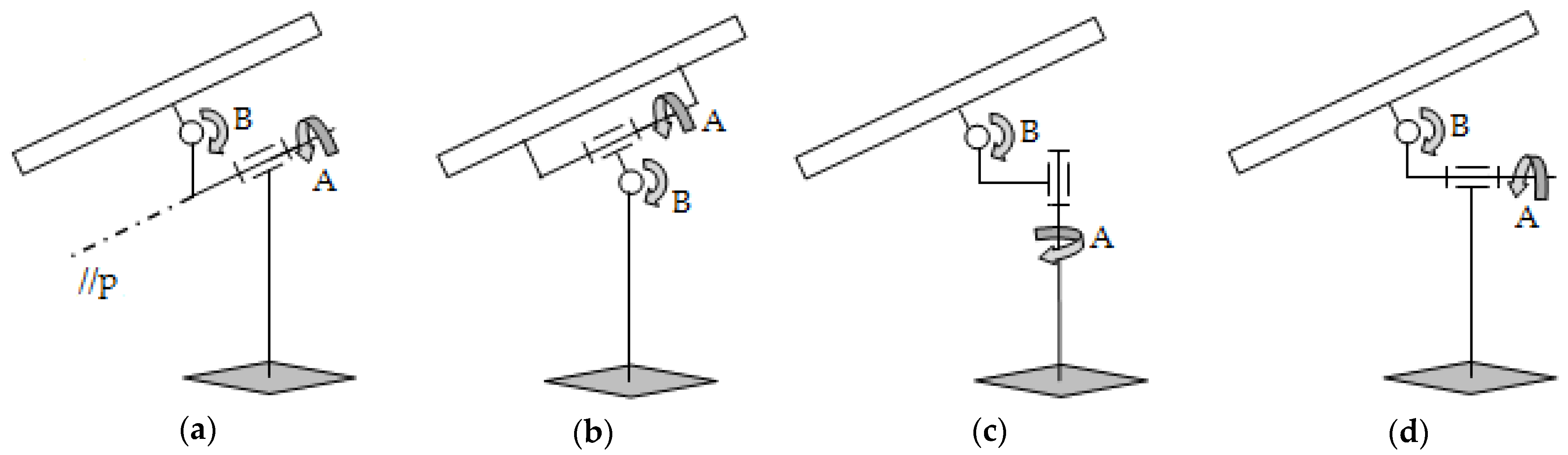In Figure 1, these types of Sun tracking systems are shown schematically, the projection corresponding to the vertical plane to which the east–west axis is normal; “A” is used as notation for diurnal motion, and “B” is used for elevation motion.

The equatorial tracking systems (Figure 1a) have as the fixed (primary) axis the one of diurnal motion, which is parallel to the polar (“p”) axis, which is why these systems are also called polar systems. The elevation movement’s axis is variable depending on the diurnal axis. The main advantage of these systems is that the sun tracking is very precise, and the movements of the PV module are able to accurately replicate the rotations in the Sun–Earth astronomical system. Thus, the two movements (diurnal and elevation) are independent (should not be correlated), which simplifies their control.

The fixed axis of the pseudo-equatorial tracking systems (Figure 1b) is the elevation movement’s axis, which is placed horizontally, parallel to the east–west axis. This solution (which is obtained by reversing the order of the rotation axes relative to the equatorial system) is simpler from a construction point of view, as well as more stable (it does not require rigorous balancing), but it does entail frequent orientation along the elevation axis (especially during warm seasons).

The azimuthal tracking systems (Figure 1c) have as the fixed axis the diurnal (azimuthal) movement’s axis, which is placed vertically (perpendicular to the observer’s plane). The elevation movement’s axis varies depending on the diurnal axis, with a correlation of the two movements throughout the day being necessary to obtain the optimal incidence of sunlight. Azimuthal-oriented systems have the stability of the structure as a core advantage.

In pseudo-azimuthal tracking systems (Figure 1d), the fixed axis is also that of diurnal motion, but which here is placed horizontally (parallel to the south–north axis), with the elevation motion’s axis being variable depending on the primary axis’ position. These systems also need a daily correlation of movements but do have the advantage of a very stable structure.

Another classification of Sun tracking systems can be made according to the number of PV modules and their arrangement, as follows: systems for separate (individual) PV modules—the modules are mounted individually, and they are actuated from their own motor sources (one or two, by case, for each module); systems for PV module strings—the modules are mounted individually, but actuation is conducted simultaneously from the same motor source(s) by means of motion transmission mechanisms (frequently based on transmissions with linkages, belts, or chains) [51]; systems for PV module platforms—the PV modules are arranged on a common frame, which is directly driven by the motor source(s) [52]; and systems for string platforms, which combine the features of systems for strings and platforms—the PV modules are mounted on individual strings, which in turn are arranged on a platform-like structure (diurnal movement is performed as in platform-type systems, and elevation movement as in string-type systems) [53].

The evaluation of the behavior and efficiency of the Sun tracking systems is frequently addressed in the literature both by using theoretical and experimental models. At the same time, the increasingly frequent use of modeling, simulation, and optimization tools in a virtual environment is noted. The detailed presentation of a software platform for virtual prototyping is carried out in [54], and several representative applications in the design process of mechanical/mechatronic systems from various fields (such as renewable energy systems and automotive engineering) are rendered in [4,34,55,56,57,58] precisely with the idea of showing the important advantages that the use of such powerful and effective testing instruments bring.

Based on that previously mentioned, in the present work, the simulation and optimization of an equatorial dual-axis tracking system is carried out, the application being made for an individual module-type system. The proposed Sun tracking system is operated by using two linear actuators, one for each of the two movements (diurnal and elevation). The constructive solution is a relatively simple one, which does not require additional elements or mechanisms to transmit the movement from the linear actuators to the PV module, which makes the cost of the system relatively low.

With reference to the research methodology, the proposed tracking system is approached in the modern concept of mechatronic product design. On the other hand, the need for a unitary algorithm for analysis and optimization led to the modeling of the tracking mechanism as a multi-body system. Based on the two adopted concepts (mechatronic system and multi-body system), the frame for the comprehensive approach of the tracking system in terms of functionality was ensured. Equally important are the tools used to achieve the research objectives, based on simulation and optimization in a virtual prototyping environment with the help of computer-aided engineering (CAE) software solutions, which translate into the creation of accurate digital models and their use in virtual experiments that reproduce the real phenomena.

In this regard, the virtual prototyping platform used for the research depicted in this work integrates the following types of CAE software solutions: CAD (Computer-Aided Design), MBS (Multi-Body System), and DFC (Design for Control). The CAD software (namely, CATIA V5—Computer-Aided Three-Dimensional Interactive Application) was used to create the 3D geometric model of the tracking system, which provides information about the mass and the inertia properties of the parts. The MBS software (ADAMS 2005r2—Automatic Dynamic Analysis of Mechanical Systems), which represents the central, integrative, component of the virtual prototyping platform, was used for the dynamic modeling, analysis, and optimization of the mechanical device of the tracking system. The DFC software (EASY5 2005r1.3—Engineering Analysis System) was used for designing the control system block diagram, including the controller that adjusts the operation of the electrical device.

Within the virtual prototyping platform, the communication between the CAD and MBS programs is a unidirectional one, in the sense that the CAD model is transferred for integration at the level of the dynamic model conceived in the MBS software. On the other hand, there is a bidirectional communication between the MBS and DFC programs (i.e., the outputs from MBS are inputs in DFC, and vice versa), as explained in Section 3 of the work. The process of virtual prototyping is approached by going through three specific stages, namely, modeling, simulation (testing), and optimization. During the modeling stage, the specific components of the tracking system (bodies, connections, actuating elements, and control elements) are created. The output from modeling is the initial virtual model, which is then simulated with the purpose of evaluating its behavior. Finally, the virtual model is subject to optimization, which aims to improve the behavior/efficiency of the tracking system in connection with the specifics of the addressed subsystem, as explained below.

Firstly, the goal of optimizing the mechanical device subsystem was to determine the optimal arrangement of the two linear actuators so that the PV module can go through the necessary angular movement fields, simultaneously with the minimization of the energy consumption for achieving the tracking, while respecting some functional and constructive constraints. Secondly, the goal of optimizing the control device subsystem, which is based on an open-loop tracking strategy, was to minimize the tracking errors (the losses of incident solar radiation caused by the not very precise positioning of the PV module relative to the Sun’s position) through the optimal design of the control elements, that is, the PID (Proportional–Integral–Derivative) control loop controllers employing feedback. Thirdly, the optimization of the bi-axial tracking program (which provides the input signals in the control system model, representing the imposed time variation laws for the diurnal and elevation angles of the PV module) is carried out by an original (as well as effective) approach, aiming to maximize the energy gain of the PV system by maximizing the amount of incident solar radiation on the PV module surface, all within the virtual prototype that integrates the mechanical and control models.

Concluding, the novelty and contribution of the work can be summarized by the following main elements (with reference both to the tracking mechanism itself and to the way in which it was optimally designed, based on the three-step optimization sequence mentioned above):

▪

The functional and constructive solution of the equatorial solar tracker, both from the point of view of the mode in which the actuating is carried out as well as regarding the adopted counterweight balancing solution, which ensures the static and dynamic stability of the system, as well as a minimum energy consumption for achieving the Sun tracking;

▪

The optimization technique/algorithm based on the parametric design tools provided by ADAMS, which was applied to optimally design the three distinct components of the tracking system, namely, the mechanical device, the control system, and the tracking program, each with specific peculiarities in terms of design objective, design variables, and design constraints;

▪

The integration of the mechanical device with the control system from the level of the virtual prototype (in a mechatronic concept), thus minimizing the risk that the control law is not accurately followed by the tracking mechanism;

▪

The way in which the optimization process of the bi-axial tracking program is configured and carried out, by using a model that integrates both the tracking mechanism itself and a numerical algorithm for estimating the amount of incident solar radiation, all within the MBS virtual environment (to the best of our knowledge, in the literature, there are no similar approaches by other authors).

2. Optimal Design of the Mechanical Device

As mentioned before, from the point of view of tracking accuracy and the complexity of the tracking program, and therefore of the control system, the most advantageous type of dual-axis system is the equatorial one, in which the primary axis (that of diurnal movement) is positioned parallel to the polar axis corresponding to the geographical location. Thus, starting from the schematic representation in Figure 1a, and choosing linear actuators as motor sources for the two specific movements (diurnal and elevation), the 3D model of the proposed system (shown in Figure 2) was developed using the MBS program ADAMS. When dimensioning the system (and therefore its elements), it was considered that it will orient an ISTAR SOLAR (IS-P) photovoltaic module, with the active surface of 1.26 m², and a conversion efficiency of about 15%. This type of module was chosen because it has already been used in several applications (including practical implementations) within the Faculty of Product Design and Environment at the Transilvania University of Brașov.

It was decided to operate the system by means of linear actuators, where the active/moving element of the actuator (i.e., the piston) acts directly on the rotating element (the module frame, for the elevation movement, or the intermediary support, for the diurnal movement) because this solution, compared to the actuation by rotary motors, simplifies the constructive solution of the revolute joints/couplings (through which the tracking according to the two axes of movement is carried out), and at the same time it ensures an increased rigidity of the system. It should also be mentioned that the linear actuators integrate screw-nut-type mechanisms, which ensure the irreversibility of the movement (by self-locking) in the stationary positions of the system (between actuations) or when external perturbations (e.g., wind) occur.

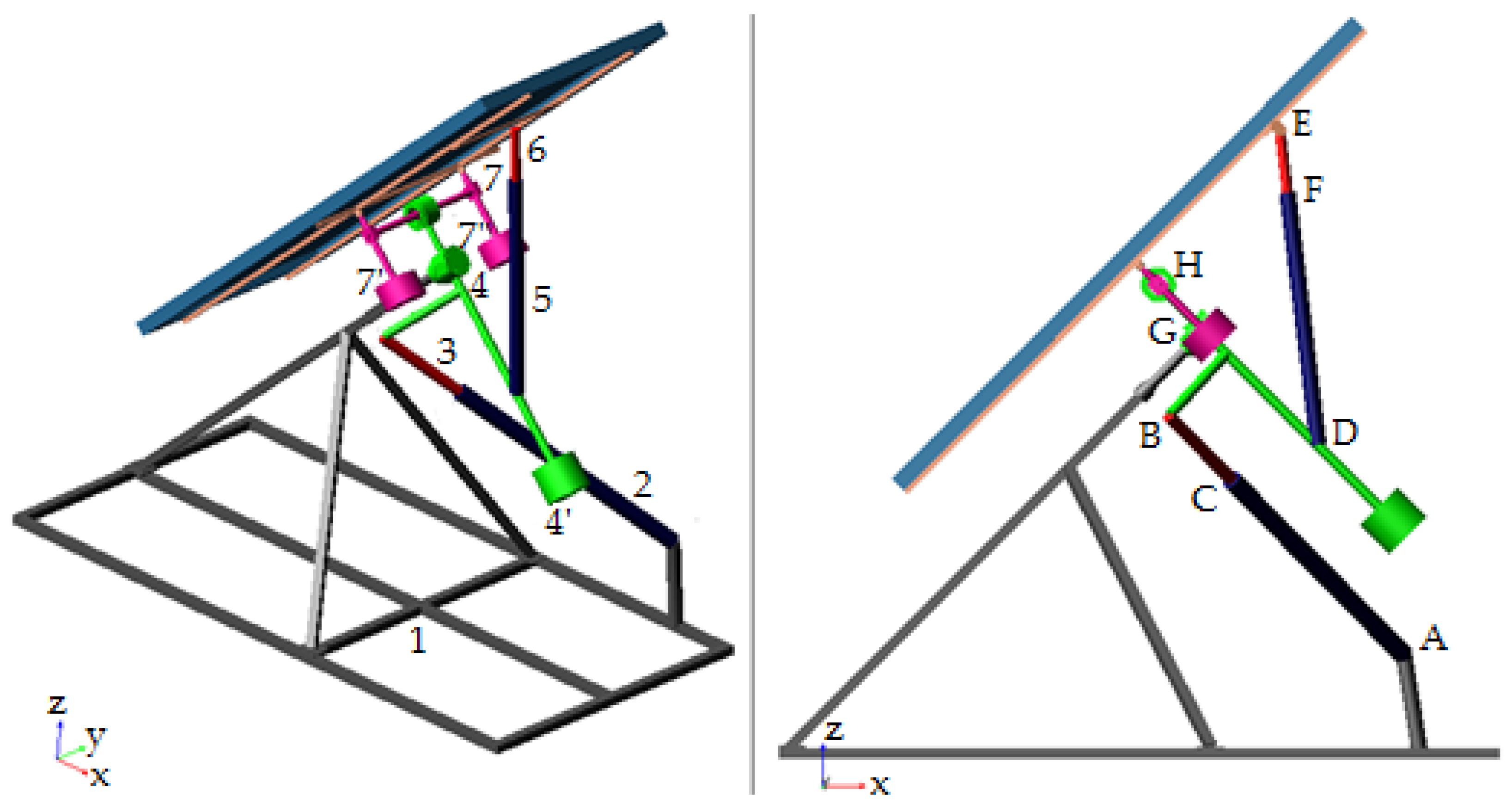
The proposed equatorial dual-axis tracking system is made up of seven bodies (parts), as follows (see the corresponding notations in Figure 2): 1—sustaining support (which is rigidly connected to the ground); 2 and 3—cylinder/housing and piston of the diurnal movement actuator; 4—intermediary support; 5 and 6—cylinder/housing and piston of the elevation movement actuator; and 7—PV module frame, to which the shaft of the elevation movement is also attached.

The two components of the diurnal movement actuator are connected by spherical joints to the sustaining support (joint A) and to the intermediary support (joint B). Similar types of couplers were used to connect the elevation movement actuator to the intermediary support (joint D) and to the PV module frame (joint E). Cylindrical couplings are used to connect the component parts of the actuators to each other (joint C and joint F). In addition to these connections, there are the rotation couplings through which the two movements in the equatorial dual-axis system are actually performed, the diurnal movement (joint G) and the elevation movement (joint H).

For a better balancing of the tracking mechanism, a system of counterweights was added, as follows: the counterweight (4′) mounted at the rear end of the intermediate support rod, through which balancing is achieved on the diurnal movement axis; and the group of two counterweights (7′–7″) mounted by roads at the ends of the shaft for the elevation movement, through which balancing is achieved on the elevation axis. The sizing and placement of these counterweights was chosen considering the need to bring the centers of mass of the moving structures as close as possible to the corresponding rotation axis, with the aim of reducing the driving/motor forces (and therefore the energy consumption required to achieve the Sun tracking).

The linear actuators intended to be used for driving the two movements in the practical application are of the MecVel type, as follows: for the diurnal movement, MecVel L02 FCM/0300 was used, where the minimum length (in a fully compressed state) is 650 mm and the maximum stroke is 300 mm; and for the elevation movement, MecVel L02 FCM/0200 was used, having a minimum length of 550 mm and a maximum stroke of 200 mm. Both actuators include magnetic limit switches and encoders. In the virtual model shown in Figure 2, there are simplified geometric representations of these types of actuators.

The goal of optimizing the mechanical device of the dual-axis tracking mechanism is to determine the optimal layout of the two linear actuators. The optimization study is performed separately on the two movement subsystems (diurnal and elevation) as long as there are no dependencies between them. The two optimization problems are of the mono-objective type, with design constraints (for avoiding unrealistic designs), which are defined as follows:

-

The design objective (DO) is to minimize the root mean square during simulation (i.e., the square root of the arithmetic mean of the squares of the values) of the driving/motor forces required to orient the PV module along the two movement axes;

-

The design variables (DVs), i.e., the independent parameters of the optimization process, are represented by the global coordinates of the points where the spherical couplings (joints) through which the linear actuators are connected to the following adjacent elements: the sustaining support (point A) and intermediary support (point B) for the diurnal movement actuator, and the intermediary support (point D) and module frame (point E) for the elevation movement actuator;

-

The design constraints (DCs): respecting the minimum length of the actuator, when it is fully retracted/compressed (DC_1); respecting the maximum length of the actuator, when it is fully extended (DC_2), which basically defines the maximum stroke of the actuator (according to the technical specifications of the two linear actuators, MecVel L02 FCM/0300 and MecVel L02 FCM/0200); and maintaining the transmission angle within acceptable limits, so that there is no risk of self-locking of the mechanism specific to the movement subsystem (DC_3).

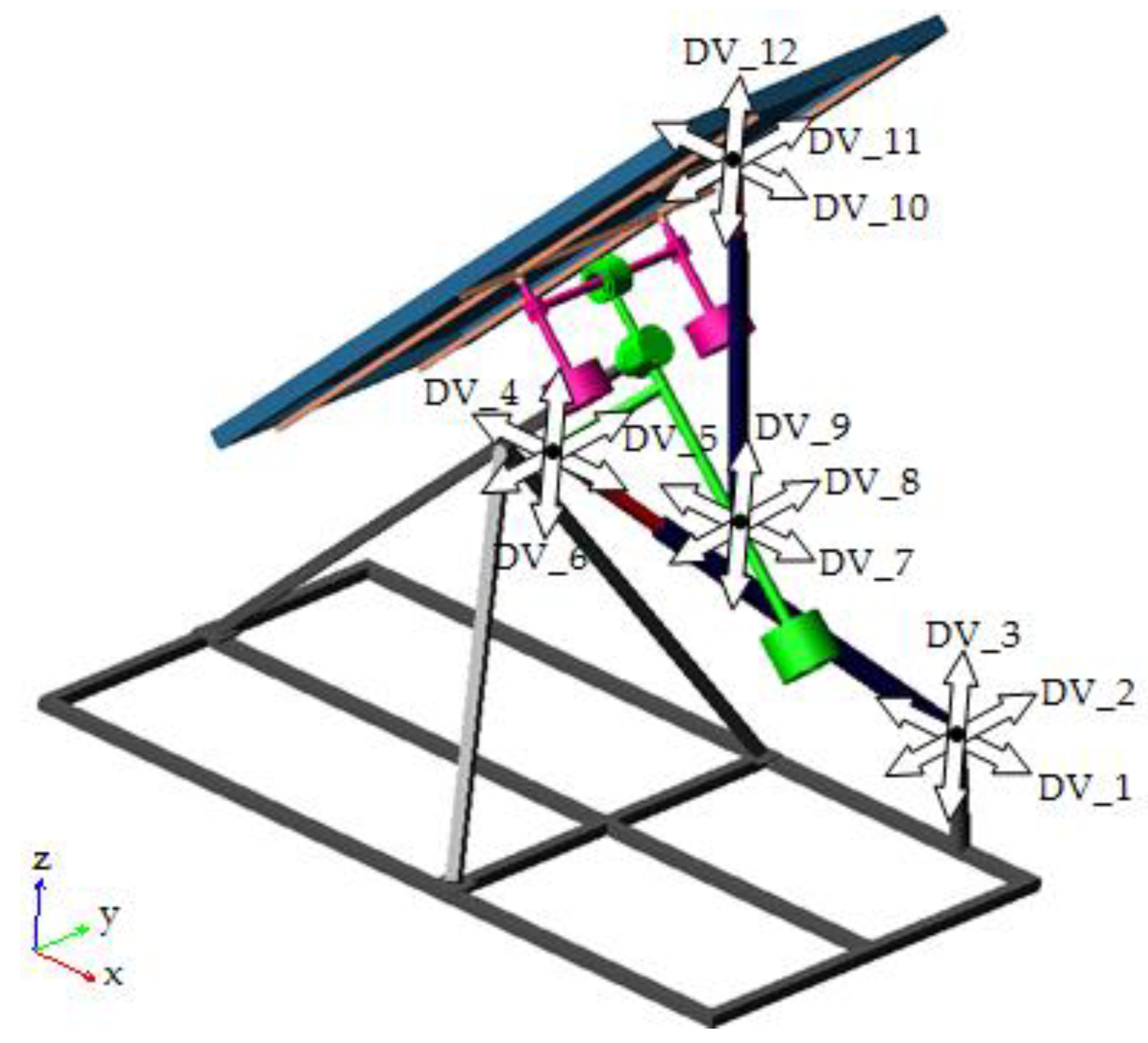
The global reference frame xyz (to which the coordinates of the design points are reported) has the axes oriented in the following way (see Figure 2): x—longitudinal axis, positive towards the back of the system; y—transverse axis, positive towards the right; and z—vertical axis, positive upwards. In these terms, the design variables in the two movement subsystems (six per subsystem) are those presented in

Table 2. Design variables for the optimization process of the mechanical device.

Global Coordinate	Design Point
	A	B	D	E
x	DV_1	DV_4	DV_7	DV_10
y	DV_2	DV_5	DV_8	DV_11
z	DV_3	DV_6	DV_9	DV_12

(the notation in the form DV_n is the one used in ADAMS). The twelve design variables are also represented/marked in a graphical form on the MBS model of the tracking mechanism (Figure 3) through arrows that indicate the direction in which the design variables change, according to the three axes of the global reference frame. Each design variable is modeled by its initial (standard) value, and the specific variation range/domain, which is defined by the minimum and maximum values of the variable. So, relative to the initial value, in the optimization process, each design variable moves both in the sense of increasing and decreasing its value on the corresponding axis. When establishing the boundaries of the variation domains, the requirement that the tracking system remains within rational/reasonable constructive limits was considered.

The coordinates of the points where the cylindrical couplings between the two components of each actuator (piston and cylinder) are located (C/F) will result by means of parameterization expressions, so that these points are permanently on the axis defined by the two ends of each actuator (A–B/D–E), at an imposed distance from one of these ends, for example, the lower end of the actuator (A/D). These expressions have been modeled by using the predefined function LOC(ATION)_ALONG_LINE(Object for Start Point, Object for Point on Line, Distance), as follows: point C—LOC_ALONG_LINE(A, B, 550); and point F—LOC_ALONG_LINE(D, E, 450).

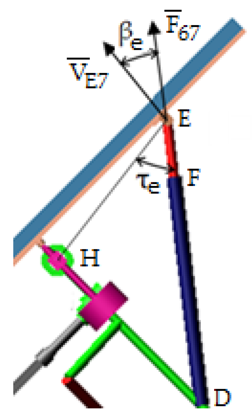
The transmission angles are defined as the complements of the pressure angles in the two motion subsystems. The pressure angle is defined as the angle between the direction of the force with which the actuator (more precisely, its piston) pushes or pulls the actuated element and the direction of the linear velocity at the actuation point on that element. Figure 4 shows the pressure (β_e) and transmission (τ_e) angles from the elevation subsystem. Similarly, the two angles in the diurnal motion subsystem are defined (β_d, τ_d). The design constraints DC_3 were modeled by reference to the transmission angles, which are easier to measure than the pressure angles, as they are measured between points already existing in model, i.e., β_e = ∠DEH and β_d = ∠ABG.

In ADAMS, the design constraints have a special meaning in that each constraint generates an inequality equation, the constraint being considered to be satisfied as long as the function by which it is defined remains negative or at the null limit. In these terms, the functions by which the above described design constraints were modeled have the following forms: DC_1 = 650 − |AB|, DC_2 = |AB| − 950, and DC_3 = 10 − τ_d (or τ_d − 170, by case/configuration) for the diurnal movement subsystem; and DC_1 = 550 − |DE|, DC_2 = |DE| − 750, and DC_3 = 10 − τ_e (or τ_e − 170) for the elevation movement subsystem. Concerning the transmission angle, theoretically, the mechanism self-locks in the positions where the transmission angle has the values 0° (the two axes between which the angle is measured are overlapped) and 180° (the two axes are in extension). For operational safety reasons, the transmission angle is limited to values greater than 0° (that is 10°) and less than 180° (that is 170°); in other words, a safety margin of 10° was considered for both possible configurations.

From the point of view of diurnal movement, the maximum theoretical angular domain is 180° (90° to the east and all the same to the west, relative to the noon position, when the module is facing south, so the diurnal angle is zero). However, based on the research carried out by the author in previous works [21,51,59], it was found that for the geographical area of Brașov (longitude ≈ 25.6° east, latitude ≈ 45.65° north), it is not necessary to cover the entire 180° domain, and this is because in the morning, after sunrise, and in the evening, before sunset, the solar radiation gain that could be obtained by orienting the PV module is relatively low, and it does not justify the energy consumption that orientation on these intervals would imply. In this regard, an angular domain of 120° (+60° to the east and −60° to the west) was determined to be optimal, and the equatorial dual-axis tracking system proposed in this work is designed based on this functional requirement. It was established by a sign convention that the diurnal angle (denoted by ω′, considering that the corresponding angle of the sunray in the equatorial system is often denoted by ω) is positive in the morning and negative in the afternoon.

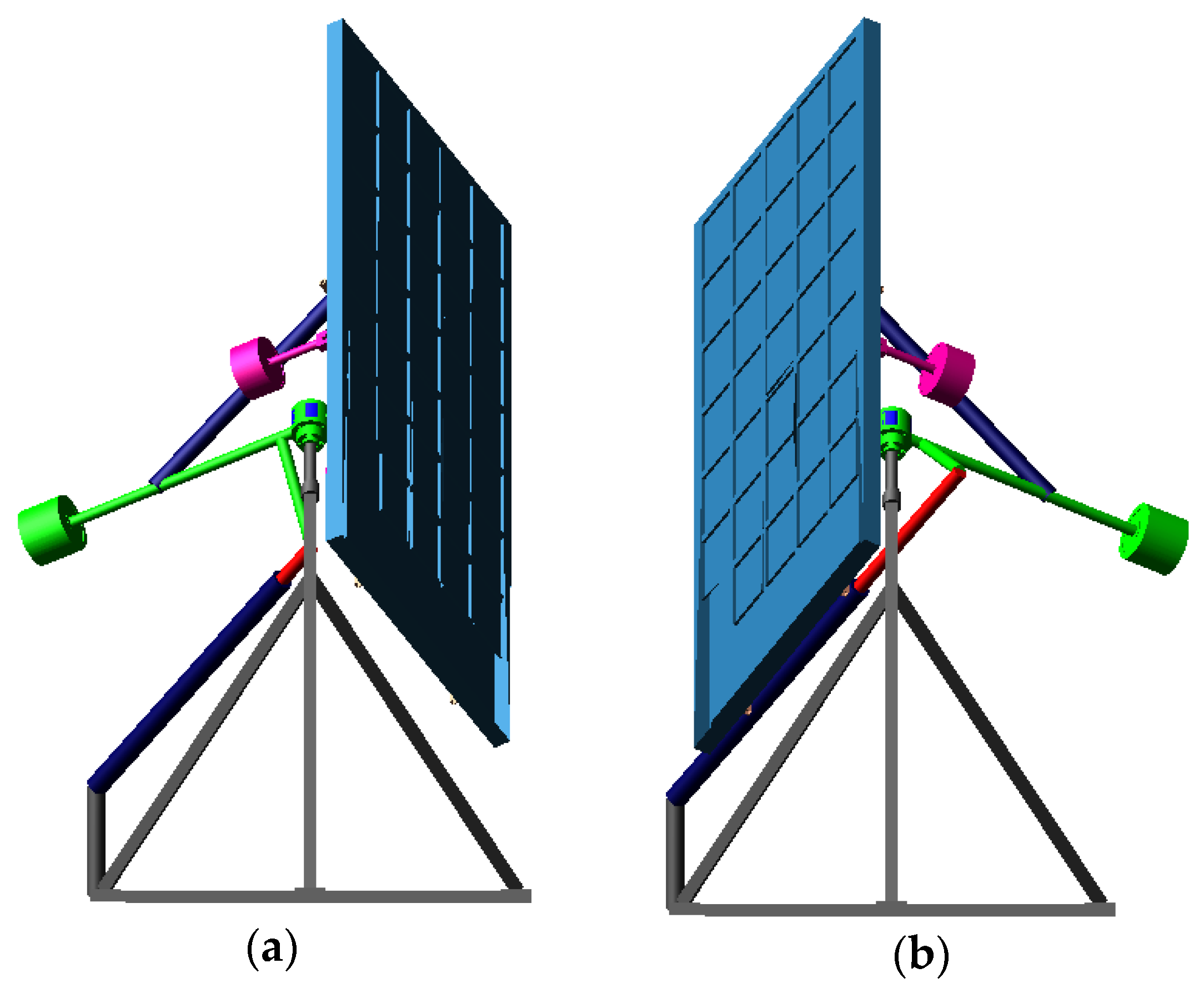
The arrangement of the diurnal movement actuator must comply with the following conditions: in the initial/morning position, where the PV module is facing east with the corresponding diurnal angle ω′ = 60°, the actuator is fully compressed, so its length (the distance between the ends, |AB|) will be 650mm; and the maximum actuator stroke of 300mm must be sufficient to rotate the PV module to the west-facing position, where the diurnal angle is ω′ = −60°. In terms of diurnal movement/angle, the two extreme (limit) positions of the PV tracking system are those depicted in Figure 5 (from the elevation movement point of view, the system is fixed in the spring/autumn equinox position, where the elevation angle is 45.65°).

The previously mentioned diurnal angle variation range, ω′ ∈ [+60°, −60°], was used in the optimization process carried out within the diurnal motion subsystem, which aimed to determine the global coordinates of the actuator end points (A and B) in the initial (morning) position, when the PV module is facing east. It was considered that the tracking is carried out with continuous movement during the longest day of the year, namely, the summer solstice day (21 June), for which the operating/actuating time is around 10 h. It should be mentioned that later, when designing the tracking program and for practical implementation, the system will be operated in steps (step-by-step) instead of continuous tracking (this will be discussed in the Section 4 of the work).

The effective optimization process in ADAMS was performed using the OPTDES-GRG (Generalized Reduced Gradient) algorithm, which requires that the design variables (DV_1–DV_6, see Table 2 for the meaning of the notations) have range limits, since it works in scaled space. The optimizer computes the design function gradients by centered differencing, which perturbs each design variable in the negative direction from the nominal value, then again in the positive direction using finite differencing between the perturbed results to compute the gradient. The differencing increment, which specifies the size of the increment to use when performing finite differencing to compute gradients, was set to 0.001; this value is first subtracted from the nominal value and then added to it.

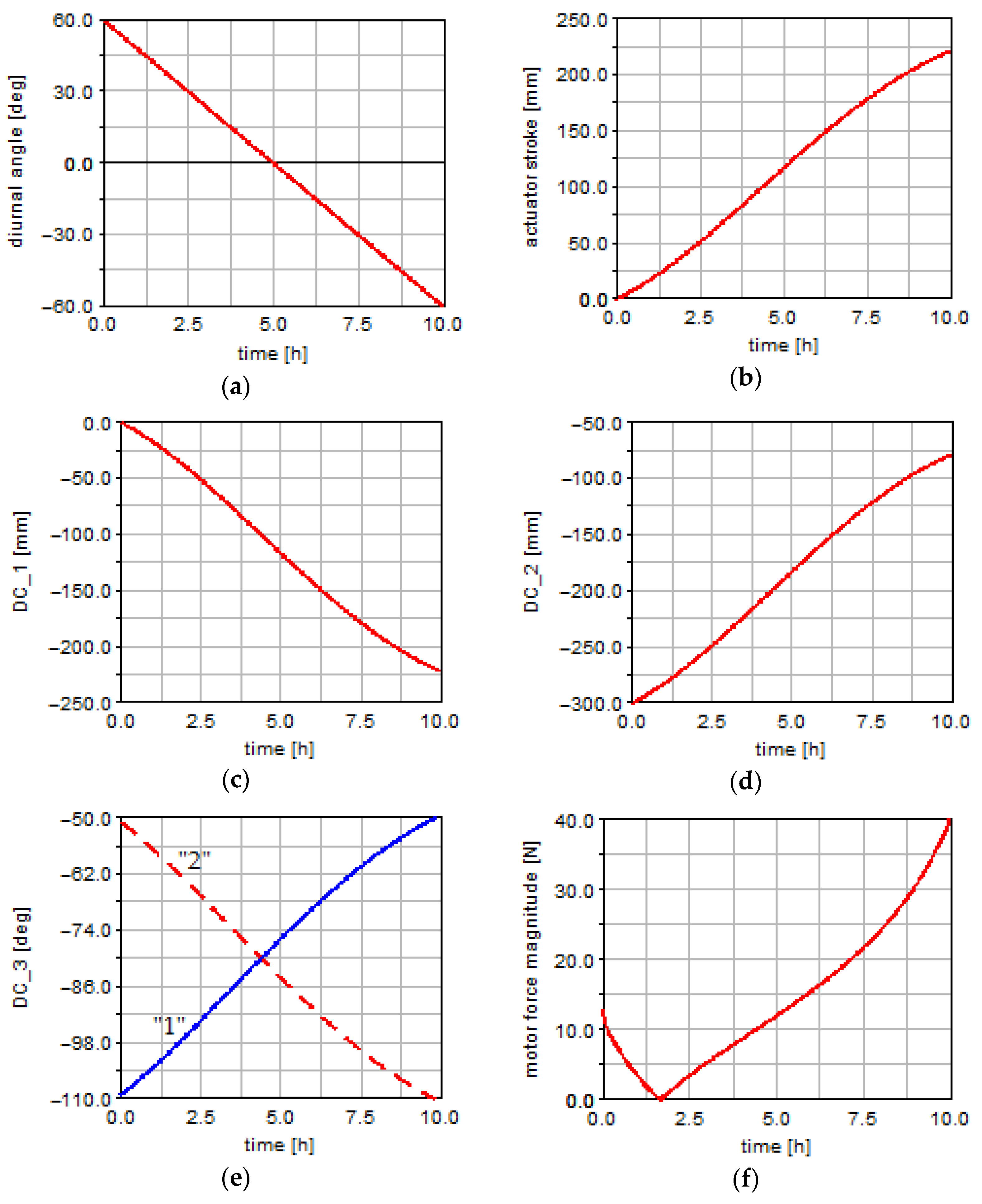
Following the optimization thus configured, the optimal arrangement of the diurnal movement actuator in the initial modeling position (the one in which the PV module is facing east—see Figure 5a) was obtained (i.e., the optimal values of the design variables DV_1–DV_6), in other words, the global coordinates of the actuator joints to the adjacent elements (the cylinder joint to the sustaining support, A, and the piston joint to the intermediate support, B), as follows: A (484.10, 348.78, 195.34) mm and B (99.67, −1.41, 585.35) mm. The most relevant results that describe the behavior of the tracking system in terms of diurnal movement are presented in Figure 6, namely, the time variations of the diurnal angle (Figure 6a), the actuator stroke (Figure 6b), the design constraints (Figure 6c–e), and the motor force magnitude (Figure 6f). For the design constraint based on the transmission angle (DC_3, Figure 6e), there are variations for both cases/configurations, namely, “1”: 10 − τ_d and “2”: τ_d − 170. As can be seen, all design constraints were respected/satisfied during the entire simulation interval (i.e., acceptable design). In the optimal design, the root mean square of the motor force (that is, the monitored parameter of the objective function during simulation) is RMS = 17.55 N.

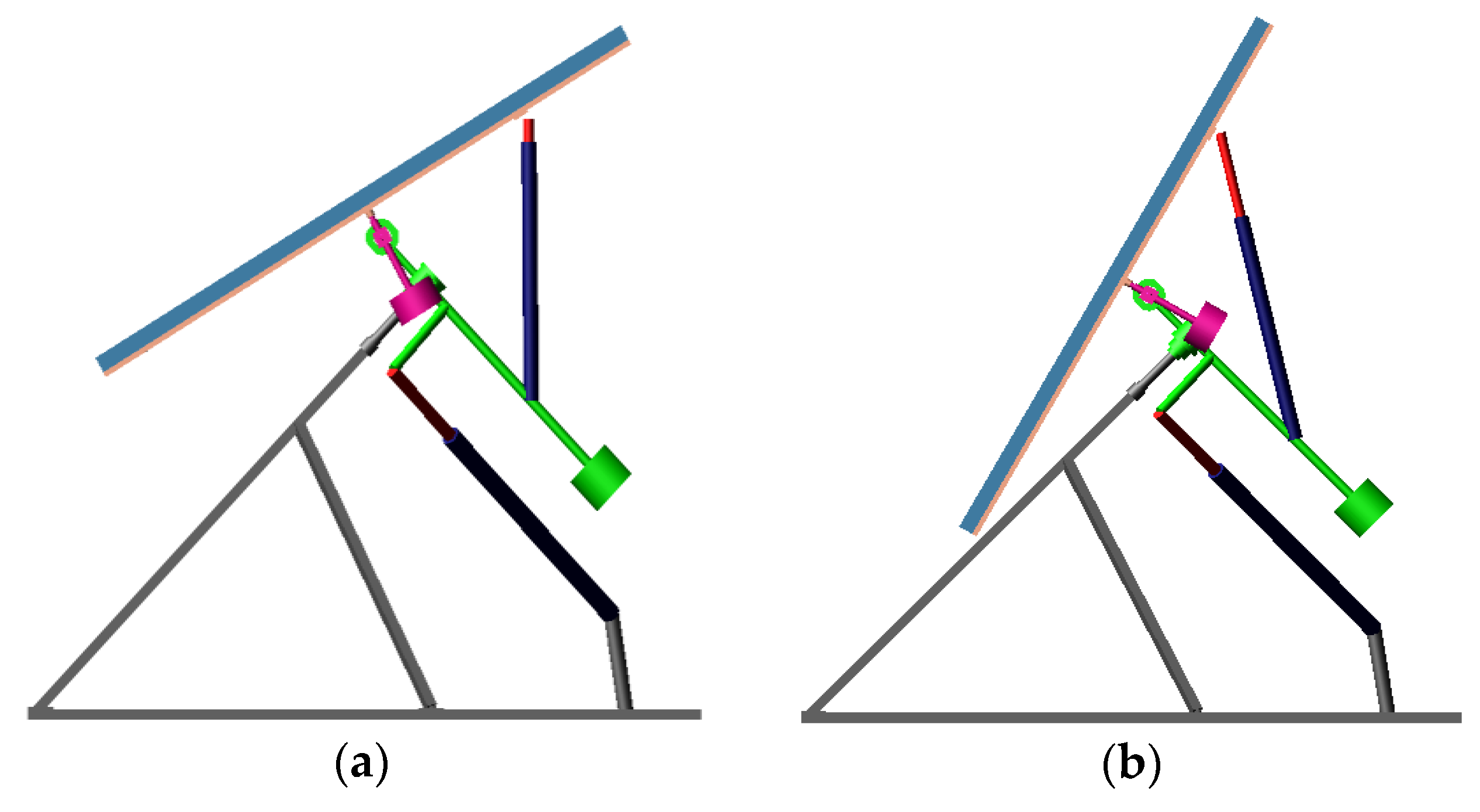
From the point of view of elevation movement, the maximum angular domain is about 47°; relative to the median position corresponding to the spring/autumn equinox (when the PV module is tilted at about 45.65°), the system must rotate by 23.45° towards the maximum (at the summer solstice) and minimum (at the winter solstice) altitudinal positions of the sun (Figure 7). It was established by a convention that the elevation angle (denoted by δ′, considering that the corresponding angle of the sunray in the equatorial system is often denoted by δ) is measured relative to the horizontal axis.

The arrangement of the elevation movement actuator must comply with the following conditions: the actuator is fully compressed in the summer solstice position (that position in which the arrangement of the PV module is closest to horizontal), where the elevation angle is δ′ = 22.05°, so its length (the distance between the ends, |DE|) in this position will be 550 mm; and the maximum actuator stroke of 200 mm must be sufficient to rotate the PV module to the position corresponding to the winter solstice (that position where the arrangement of the PV module is closest to vertical), where the elevation angle is δ′ = 68.95°. The two elevation limit positions are shown in Figure 8, where from the diurnal angle point of view, the system is fixed in the noon position (ω′ = 0°).

The previously mentioned elevation angle variation range, δ′ ∈ [+22.05°, +68.95°], was used in the optimization process carried out within the elevation motion subsystem, which aimed to determine the global coordinates of the actuator end points (D and E) in the initial (summer solstice) position, where the PV module has the closest position to horizontal (since the Sun altitude is the highest). As in the case of the optimization in the diurnal movement subsystem, here, it was also considered that the tracking is conducted with continuous movement (without stops). The time interval in which the operation occurs in the elevation movement subsystem is not relevant, so that a random interval of one hour was chosen to cover the whole angular domain of the elevation movement.

For the effective optimization within the elevation movement subsystem, the same optimization algorithm was used as for the diurnal movement subsystem, namely OPTDES-GRG with the centered differencing method. Following the optimization thus configured, the optimal arrangement of the elevation movement actuator in the initial modeling position (corresponding to the summer solstice configuration—see Figure 8a) was obtained (i.e., the optimal values of the design variables DV_7–DV_12), in other words, the global coordinates of the actuator joints to the adjacent elements (the cylinder joint to the intermediary support, D, and the piston joint to the module frame, E), as follows: D (449.47, 0.0, 598.22) mm and E (85.83, 0.0, 1010.88) mm.

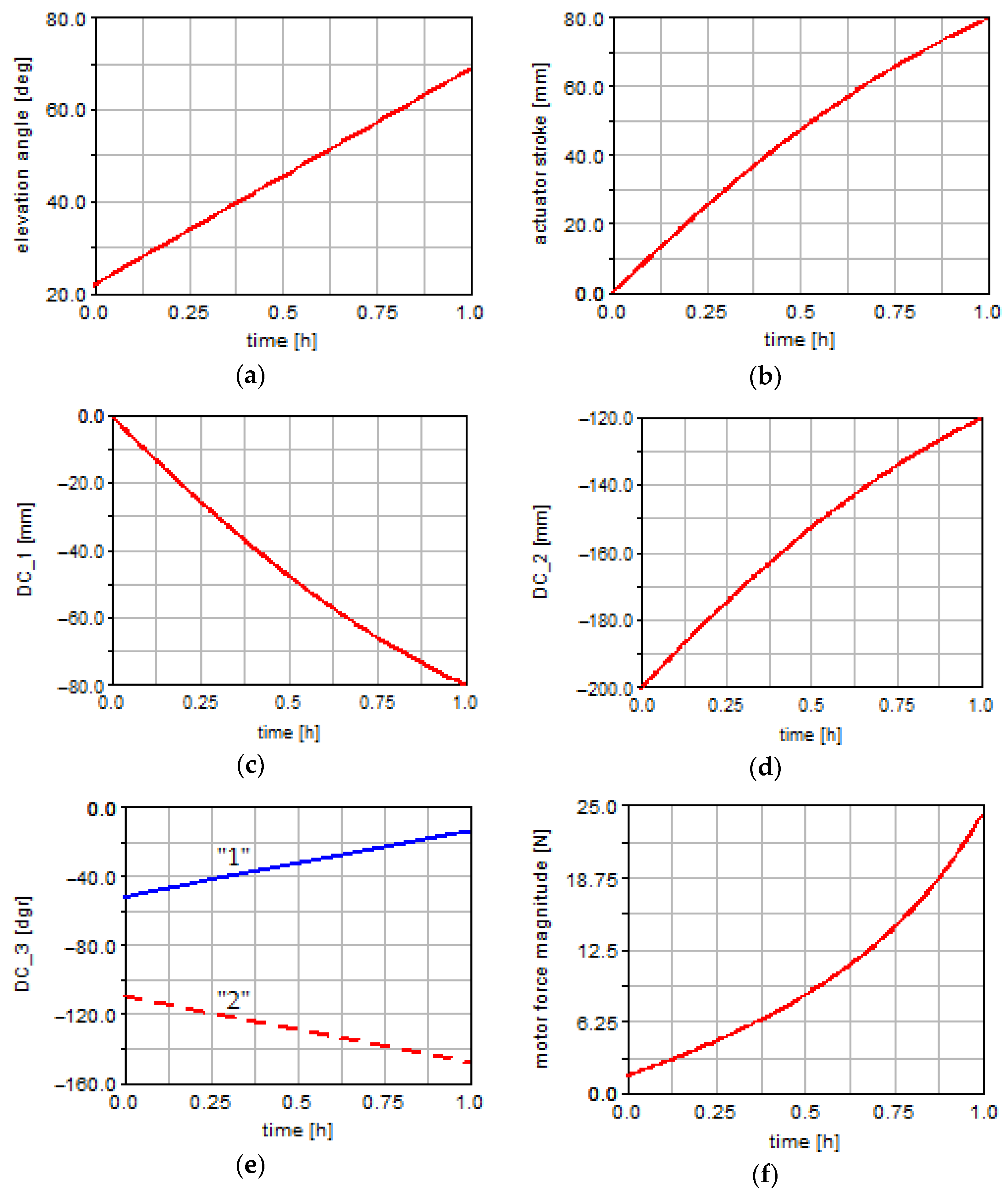
The most relevant results describing the behavior in the elevation subsystem are shown in Figure 9, namely, the time variations of the elevation angle (Figure 9a), the actuator stroke (Figure 9b), the design constraints (Figure 9c–e), and the motor force magnitude (Figure 9f). For the design constraint based on the transmission angle (DC_3, Figure 9e), there are variations for both cases/configurations, namely, “1”: 10 − τ_e and “2”: τ_e − 170. It can be seen that all design constraints are satisfied during the entire simulation interval. In the optimal design, the root mean square of the motor force is RMS = 11.82 N.

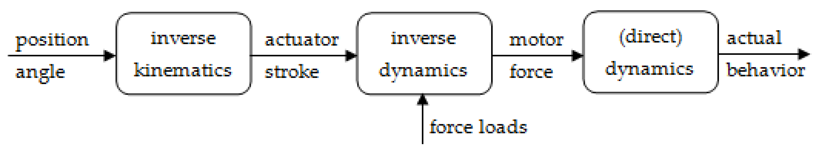
For both movement subsystems, it is mentioned that the correlation between the position angle of the PV module (diurnal or elevation, by case) and the linear stroke of the corresponding actuator was obtained through inverse kinematic analysis, while the motor forces developed by the actuators were determined by inverse dynamic analysis, based on the imposed kinematic behavior of the system loaded with forces. The analysis algorithm implemented in this regard is schematically shown in Figure 10.

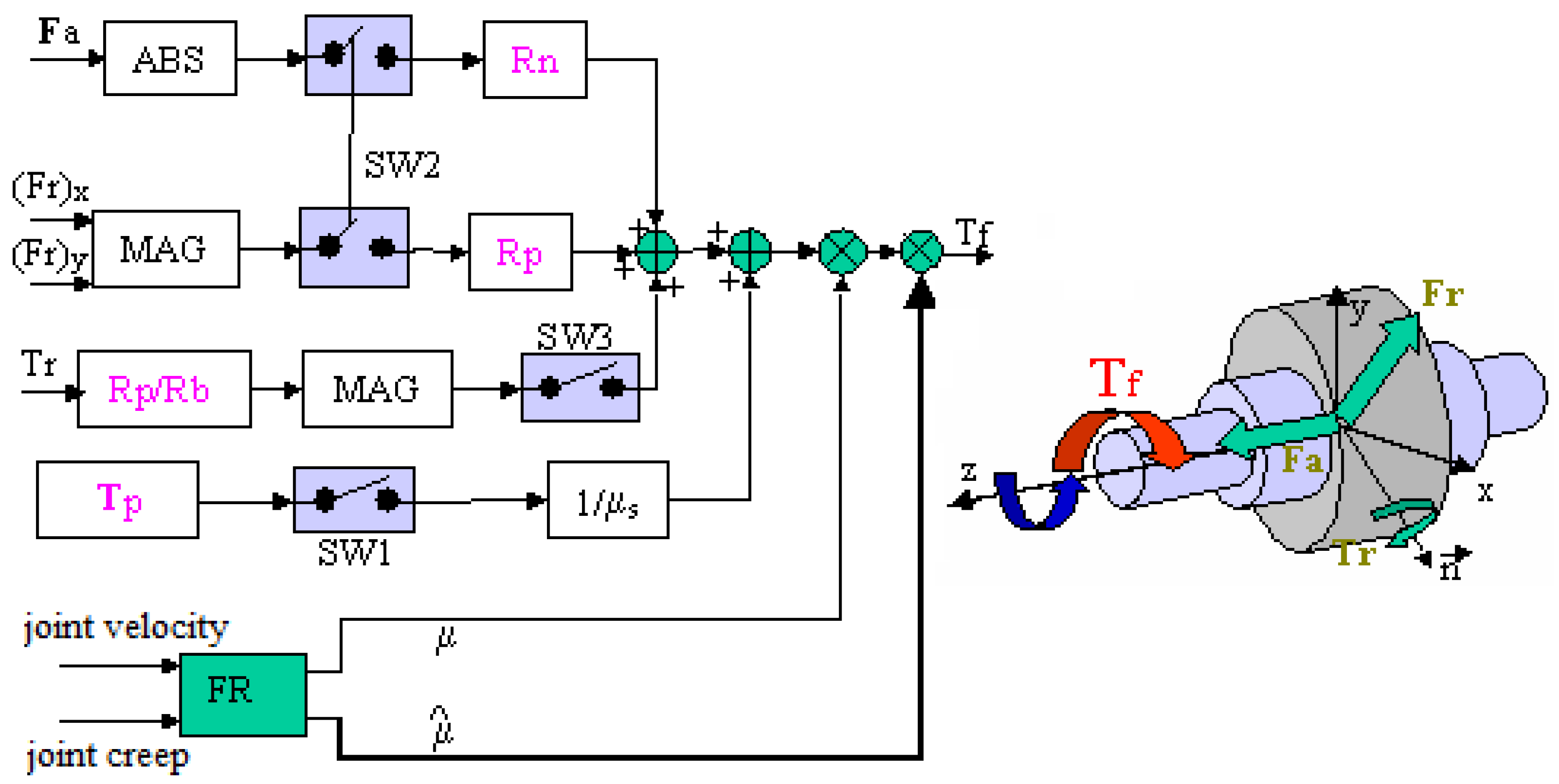
For the force loads, which represent input data in the inverse dynamic analysis, in addition to the mass and inertial forces generated by the bodies, the frictional forces from the rotational couplings (joints) through which the two movements of the PV module are realized (namely, G and H, as noted in Figure 2) are also considered; the frictions from the other joints are neglected, as they are very small. The block diagram of a revolute joint in ADAMS is shown in Figure 11, where [60] R_n—friction arm; R_p—pin radius; R_b—bending reaction arm; μ—friction coefficient (static or dynamic, by case); SW—switch block; MAG—magnitude block; ABS—absolute value block; FR—friction regime determination (dynamic friction/transition between dynamic and static friction/static friction); ⊕—summing junction; and ⊗—multiplication junction. The frictional torque in the revolute joint (T_f) is determined by the axial (F_a) and radial (F_r) joint reactions, the bending moment (T_r), and the preload torque (T_p). The force effects can be turned off by using switches.

Once the modeling of the mechanical device of the equatorial tracking system has been completed, we proceed to the optimal design of the control system, according to what is presented in the next section of the work.

3. Optimal Design of the Control System

The tracking mechanism addressed in the work is of the active type, which integrates (in a mechatronic concept) the two specific components of such a system, namely, the mechanical device and the control device. By the fact that the two components of the mechatronic tracking system are integrated and tested together at the level of the virtual (software) prototype, the risk that the control law is not accurately respected/followed by the mechanical device at the level of the physical (hardware) prototype is minimized.

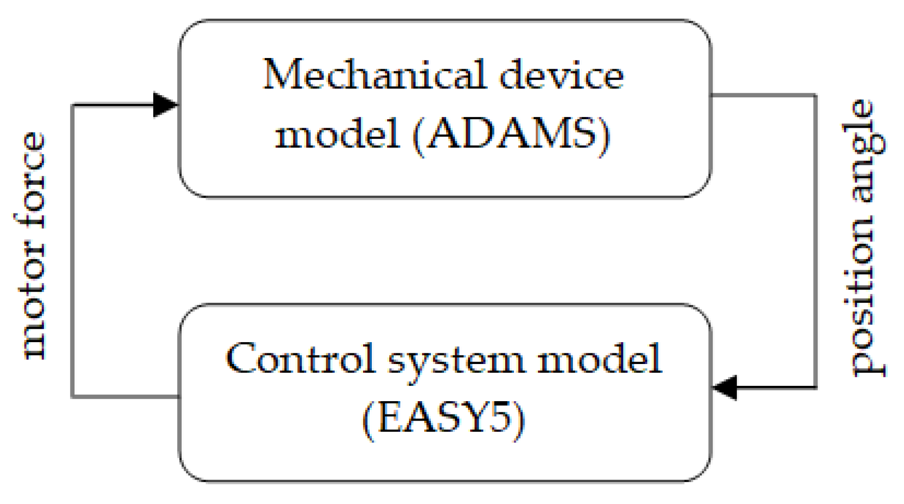
The block diagram of the control system is made with the help of the DFC software solution EASY5, and the integration with the MBS model of the mechanical device (see Figure 2), which was designed in ADAMS, was conducted with the help of the ADAMS/Controls plug-in. For controlling the movement in the diurnal and elevation subsystems of the proposed dual-axis solar tracker, open-loop strategies based on predefined tracking programs have been selected (with the remark that the optimal design of the tracking program is discussed in the next section of the work).

Control is a process in which a quantity (the controlled quantity) is continuously sensed, compared with the reference quantity, and, depending on the result of this comparison, it intervenes in order to bring the controlled quantity to the value of the reference one. The output from the control device is the input for the controlled process (the purpose of the entire control system is to drive the process so that the output from this process is identical to the reference quantity). The integration process of the mechanical device with the control system involves, in addition to designing the MBS (ADAMS) model of the mechanical device, going through the following three stages: modeling the inputs and outputs of the controlled process—the outputs describe the variables that go to the control application (the outputs from ADAMS are inputs to EASY5), while the inputs describe the variables that return to ADAMS (the outputs from EASY); designing the block diagram of the control system in EASY5 and integrating the ADAMS model in the control block diagram; and simulating the mechanical model combined with the control system model (i.e., co-simulation).

According to the proposed control strategy, for each of the two movement subsystems, there is only one input parameter in the mechanical device model, and that is the motor/driving force developed by the corresponding linear actuator. Instead, from the point of view of the outputs of the mechanical device model, their number depends on the number of control loops, in other words, the number of monitored/controlled parameters. Thus, control schemes can be defined with one, two, or three monitored parameters as follows: one-loop control schemes—a position parameter (linear or angular, as appropriate) is usually monitored; two-loop control schemes—a position parameter and a velocity parameter are usually monitored; three-loop control schemes—in addition to the parameters monitored in the two-loop schemes (position and velocity), a current-related parameter is also monitored. It is obvious that the one-loop control systems are functionally and constructively simpler, while the multi-loop control systems can provide superior stability and robust performance.

Besides the number of control loops, another important aspect in control system design is related to the type of control element (i.e., controller), which is a critical component used to regulate the behavior of dynamic system or process, one such element being required for each monitored parameter (so, each control loop). From this point of view, relatively simple controllers (amplifier or low pass filter), controllers with a more complex structure (such as PID, Proportional–Integral–Derivative), as well as intelligent controllers based on fuzzy logic (FLC) can be used.

Obviously, the type of control system and controller is established according to the specific application, the optimal variant expressing a trade-off between system complexity (which is finally reflected in cost) and performance. For the application presented in this work, based on the comparative analysis of several control schemes and elements, it was decided to use a single-loop control scheme with a PID controller, which is a control loop mechanism employing feedback that continuously calculates the error value (as the difference between the desired setpoint and the measured process variable) and applies a correction based on proportional, integral, and derivative terms. Through the optimal design of the control system (that is, by the appropriate tuning of the PID controller), the required stability and robustness characteristics are ensured without the need to use a more complex multi-loop control system.

As mentioned before, the input parameter in the mechanical device model is the motor force developed by the linear actuator, while the output parameter (which is transmitted to the control system model) is the position angle (diurnal or elevation, by case) of the PV module. In the previous section of the work, the correlation between the position angle of the PV module and the stroke of the actuator used as a motor source in the considered movement subsystem was explained (see Figure 10). In these terms, the input and output variables of the controlled process are those mentioned in Figure 12, such a scheme corresponding to each of the two movements (diurnal and elevation) of the dual-axial tracking system.

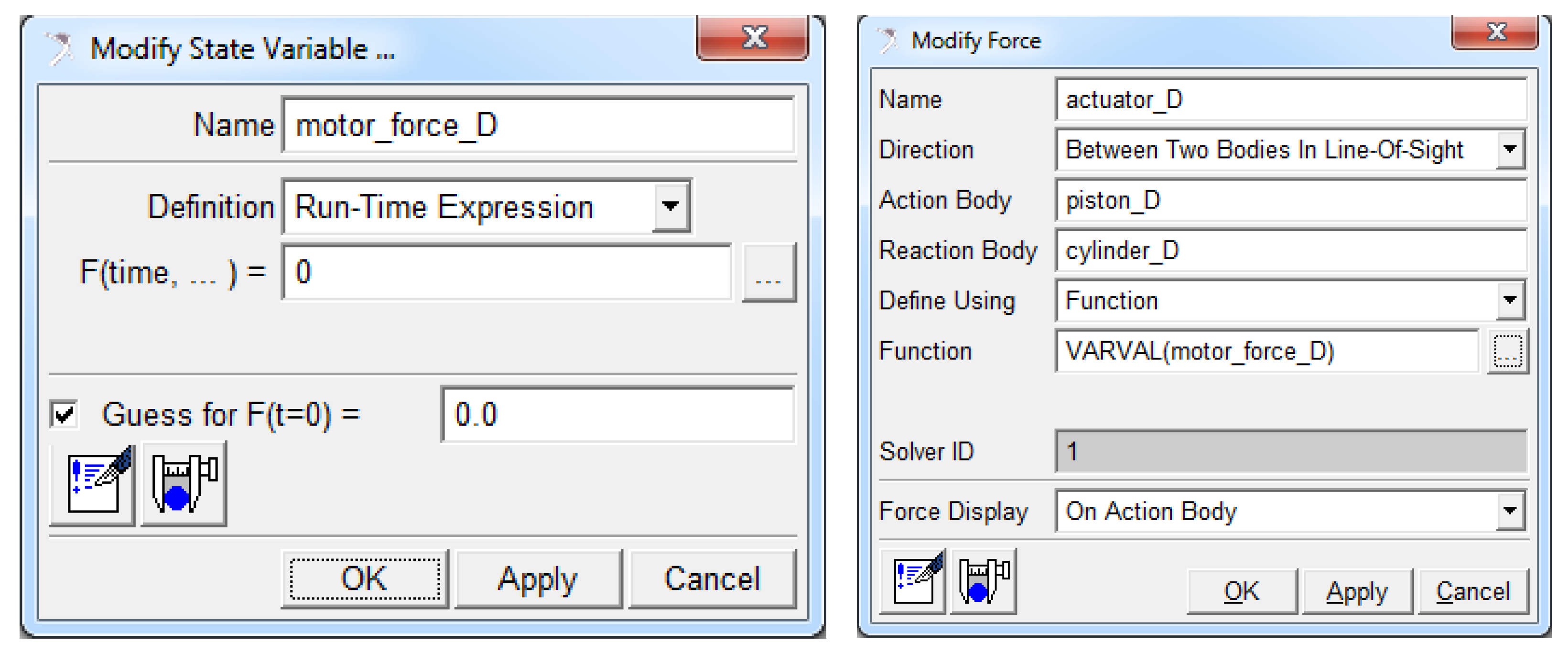
The modeling in ADAMS of the input and output state variables was carried out in the following way: the input variable, which was initially modeled with the value 0, as the current value to be generated by the control system model, was associated/assigned to the motor force generated by the linear actuator through the function VARVAL (Variable Value), as shown in Figure 13; the output variable (that is, the diurnal or elevation angle of the PV module) was modeled by using a function with the syntax AZ (From Marker, To Marker), which returns the position angle of the PV module on the desired movement axis as the angle between the coordinate system markers in the revolute joints between the intermediary support and the sustaining support (for the diurnal angle, joint G, in Figure 2) and the module frame and the intermediary support (for the elevation angle, joint H), as shown in Figure 14. 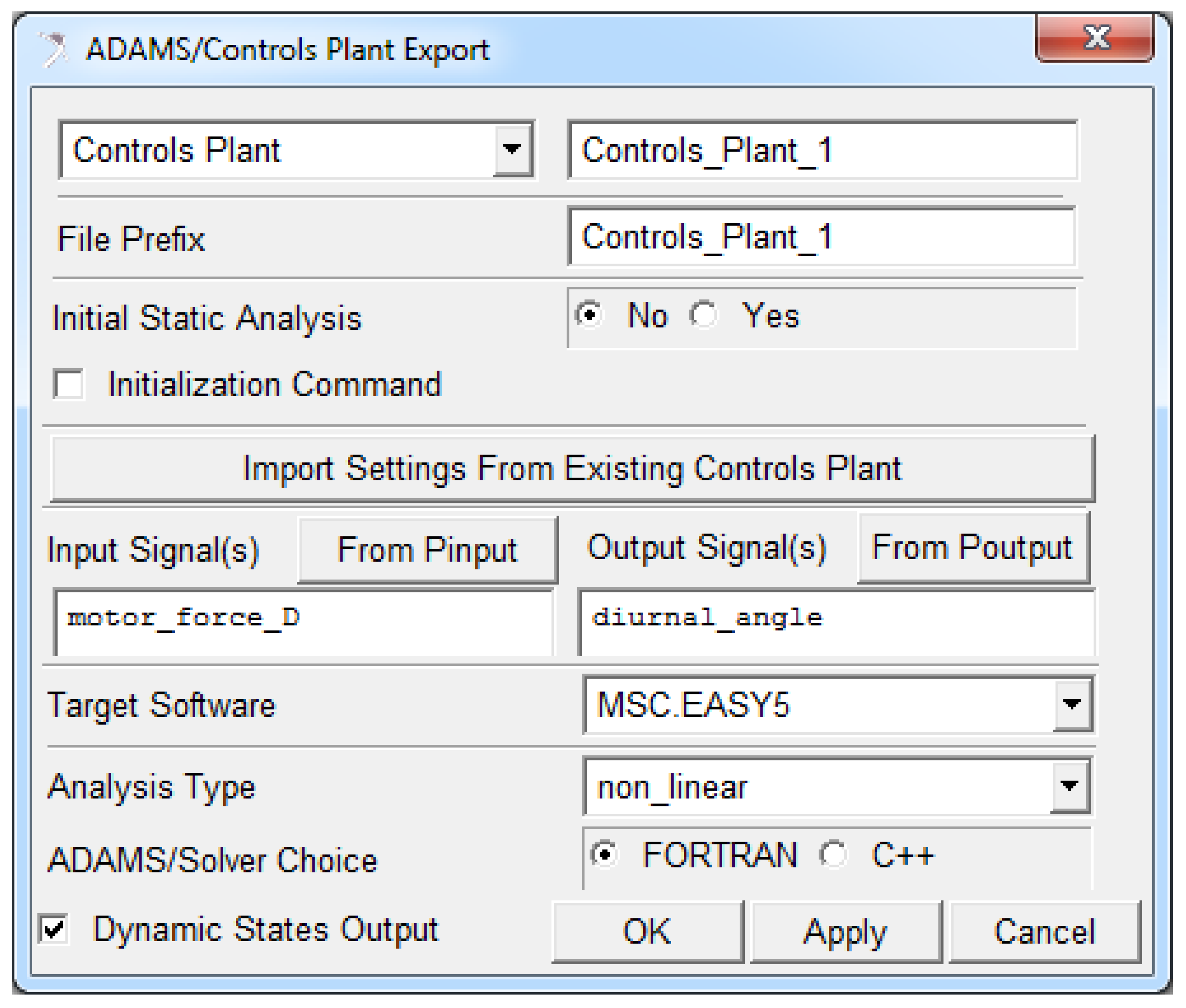The state variables thus defined were subsequently used to model the input and output plants (PINPUT1—Plant Input; POUTPUT1—Plant Output) of the controlled process, as shown in Figure 15. Further, by using ADAMS/Controls (Figure 16), the files for the control application (EASY5) have been generated, namely, a file containing the information about the input and output plants (*.inf), and a set of two files (*.cmd and *.adm) that will be used during co-simulation. Those shown in Figure 13, Figure 14, Figure 15 and Figure 16 correspond to the diurnal movement subsystem, with the modeling/settings for the elevation movement subsystem being similar.

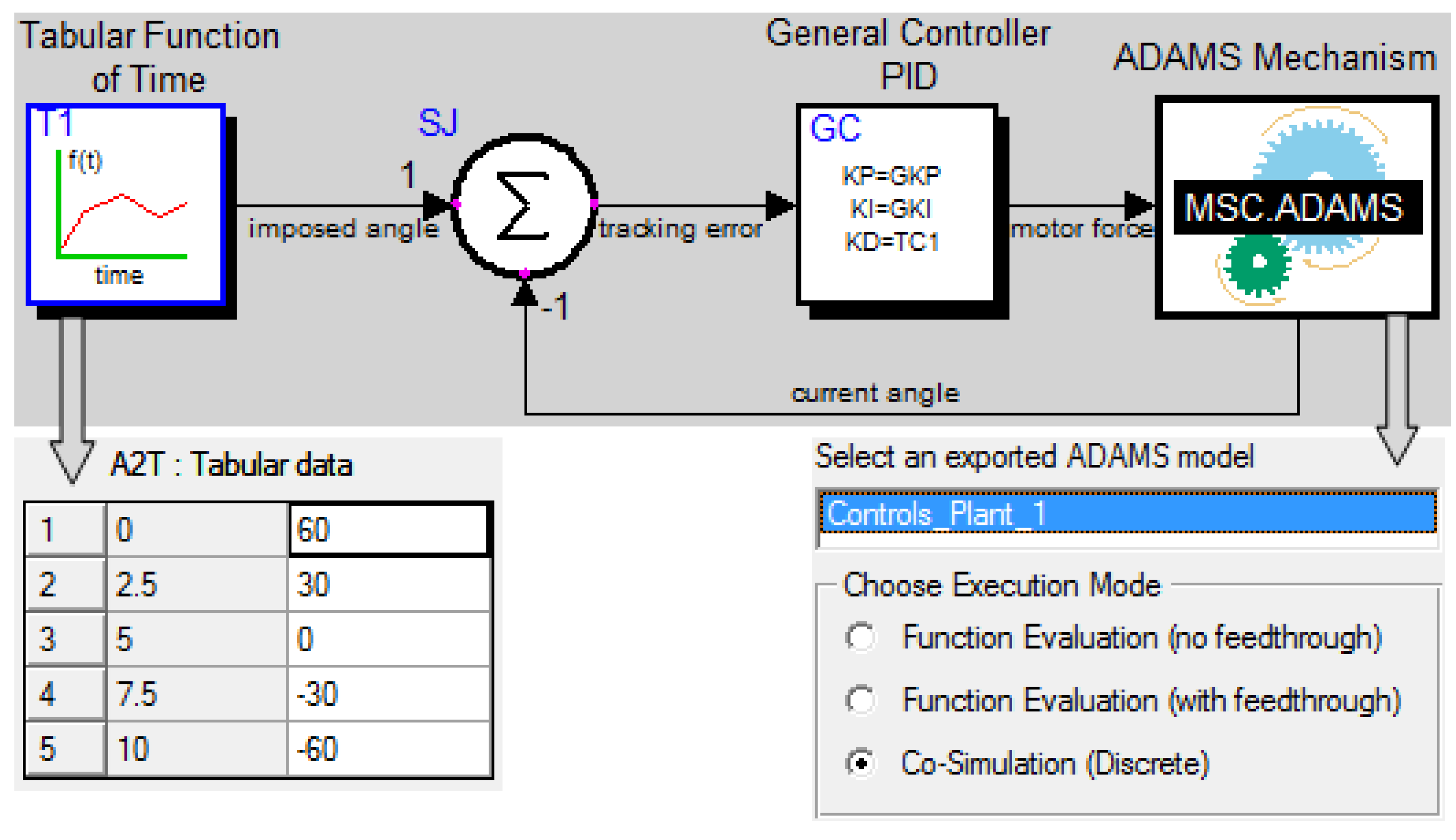
With these, the single-loop control system model designed in EASY5 is that shown in Figure 17, with each of the two movements in the dual-axial system (diurnal and elevation) being controlled by such a model. The following components can be found in the control system block diagram (the notations from EASY5 are used): ADAMS Mechanism (MSC.ADAMS), Tabular Function of Time (T1), Summing Junction (SJ), and General Controller PID (GC).

ADAMS Mechanism, which can be found in EASY5 in the form of an Extension library, is the interface block used to connect the control system model (EASY5) with the mechanical device model (ADAMS), according to the information in the *.inf file generated by ADAMS/Controls. The communication between the two models is assured by the input and output variables mentioned in Figure 12. As an execution mode, co-simulation was selected (see “Select an exported ADAMS model” extension in Figure 17), which has the effect of running the EASY5 and ADAMS models in parallel, the two solvers exchanging input and output data at a predefined rate. In addition, there are the following parameters by which the ADAMS interface block is configured: ADAMS_Animation_Mode (0/1)—to run the MSC.ADAMS simulation in the batch mode without the ADAMS model being animated (0), or to display an animation of the ADAMS model (1); ADAMS_Output_Interval—determines how often animation data are sent to the MSC.ADAMS; ADAMS_Solver (1/2)—sets the type of solver used in ADAMS, Fortran (1), or C++ (2); Communication_interval—defines the time between exchanges of data between the two solvers (EASY5 and ADAMS).

Through the control system, the value of the motor force developed by the linear actuator is computed and applied as input to the mechanical device model, which in turn returns to the control system the value of the current angle of the PV module, which is then subtracted from the imposed angle, whose value is generated by the Tabular Function of the time block. This block provides a table as a function of time, according to the tracking program for the movement under consideration. The table is defined by a number of finite positions (pairs of time—angle values), with linear interpolation being used in between. As an example, the variation law of the diurnal angle is shown in Figure 6a, which assumes the rotation of the PV module with continuous motion between the two extreme positions in Figure 5a, so in the interval ω′ ∈ [+60°, −60°], the table that generates the imposed signal is detailed in the “A2T: Tabular data” extension in Figure 17.

Summing Junction is used to compare the imposed and current/measured values of the position angle (diurnal or elevation, by case) corresponding to the considered movement. The positive input (1) in this block represents the imposed value of the angle, while the negative input (−1) corresponds to the current value achieved through the tracking mechanism, the actual operation being one of subtraction. The output from the SJ block is the tracking (positioning) error, which is to be minimized by the control system. It should be mentioned that significant tracking errors would result in losses of incident solar radiation, with a negative effect on the energy efficiency of the tracking system.

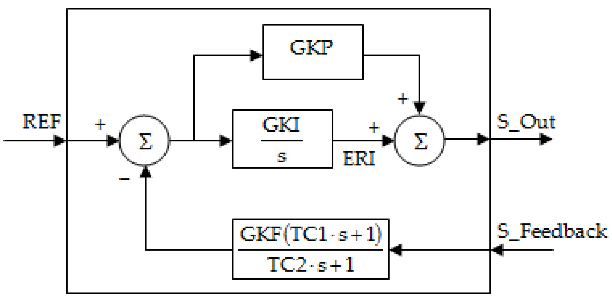
General Controller is used to model the PID position controller, which is a control loop mechanism employing feedback that continuously captures the tracking error value and applies a correction based on proportional, integral, and derivative terms. The following parameters are found in the PID controller scheme, according to Figure 18 (the notations from EASY5 are used) [61]: REF—controller input (i.e., the tracking error); S_Feedback—feedback signal; GKP—proportional control gain; GKF—feedback gain; GKI—integration control gain; TC1—derivative action time constant (which is used as a lag time constant to calculate an approximate derivative from the error signal); TC2—feedback damping time constant (which is used in the feedback to help prevent an implicit loop); S_Out—controller output (i.e., the motor force); ERI—integrated error signal; ERV—intermediate output; and s—Laplace transform.

The transfer function generated by the PID controller, which defines the relationship between the system output and input, has the following form [48]:

S_Out = ERI + GKP·[REF − FBS·S_Feedback],

(1)

where

FBS = [ERV + S_Feedback·TC1·GKF]/TC2, d(ERV)/dt = GKF·S_Feedback −
FBS, d(ERI)/dt = GK1·[REF − FBS].

(2)

By neglecting the feedback line, which (by the way the block diagram in Figure 17 is defined) is explicitly integrated into the control system model through the Summing Junction (SJ) block, the simplified form of the transfer function is obtained, as follows:

S_Out/REF = GKP·[1 + 1/(GKI·s) + TC1·s].

(3)

Tuning the PID controller can be carried out by different methods, such as root locus or frequency methods. In this work, controller tuning is approached as an optimal design process, the optimization algorithm being similar to the one used for optimizing the MBS mechanical model of the tracking system (which was addressed in the previous section of the paper). So, the optimal design of the PID controller is configured by the following: design variables—the tuning factors of the PID controller, namely, GKP (equivalent with P), GKI (I), and TC1 (D); objective function (design objective)—the tracking error; monitored value of the objective function—root mean square (RMS) during the simulation; and the optimization goal—minimization of the monitored value of the objective function.

For having access to the parametric optimization tools provided by ADAMS (with which the mechanical device model was previously optimized), it is necessary to transfer/export the control system model (Figure 17) from EASY5 to ADAMS, through an ESL (External System Library) format, as shown in Figure 19. In the transfer/export interface, the design variables (referred to as design parameters) and the design objective (referred to as display output) are specified. Afterwards, the model is imported into ADAMS in the form of a general state equation (GSE), which is based on the information stored in the external system library, as shown in Figure 20.

Thus, the parameterized model of the control system, coupled with the MBS mechanical model of the tracking mechanism, becomes available for optimization, which is of the mono-objective type, without design constraints. The optimization algorithm is that used in the optimal design of the mechanical device, namely, OPTDES-GRG with the centered differentiation method.

For both control system models, one for each of the two movements in the dual-axis tracking mechanism, the simulation is performed for a single movement step, with an amplitude of 20°, which is performed in 20 s. The movement step starts from the initial position of the system, when the PV module is in the morning position, facing east for the diurnal movement (i.e., that position shown in Figure 4a), and also when the PV module is at the maximum altitude position, corresponding to the summer solstice for the elevation movement (i.e., that position shown in Figure 7a).

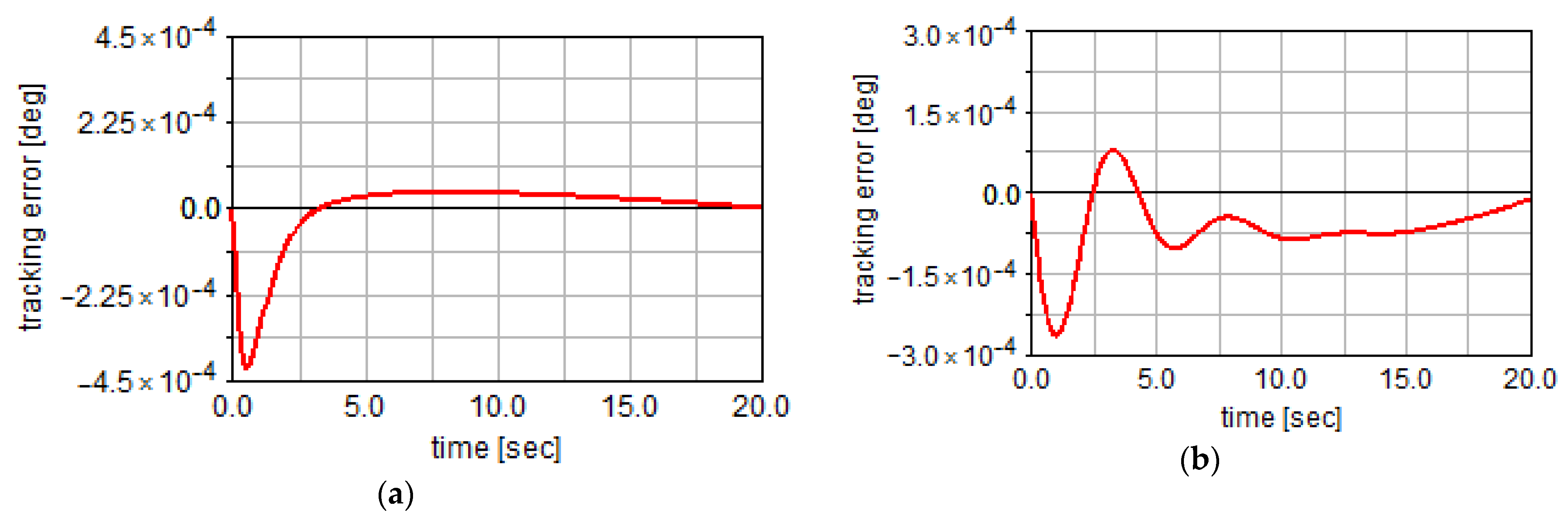
Following the optimization process configured on the basis of that previously specified, the optimal values of the tuning factors of the PID controllers resulted as follows: P_d = 4939, I_d = 4607, and D_d = 1191 for the diurnal movement controller; and P_e = 4252, I_e = 2585, and D_e = 4737 for the elevation movement controller. With these values, insignificant deviations from the imposed signals (in terms of diurnal and elevation angles) are obtained, as shown in Figure 21, and the root mean squares of the tracking errors during the simulation have very small values, RMS_d = 0.000096° and RMS_e = 0.000084°, which means that the imposed movement laws are followed accurately.

4. Optimal Design of the Tracking Program

As previously mentioned, the operation of the proposed tracking system is based on open-loop control strategy, which means that the system is designed to follow the Sun’s trajectory according to a predefined tracking program. Considering that the tracking system is a dual-axis one, the tracking program will include the time variation laws for the diurnal (ω′) and elevation (δ′) angles of the PV module. Since the two movements in the equatorial dual-axis system are independent, that is, they must not be correlated, the design of the biaxial tracking program can be conducted separately, for each of two movements (i.e., position angles). This is an important advantage of the equatorial tracking systems in relation to the other types of solar trackers schematically rendered in Figure 1.

On the other hand, in solar tracking systems, the movement can be carried out either continuously, without breaks, or in steps, i.e., step-by-step. The latter variant (i.e., tracking in steps) is the one frequently used for practical implementation, considering at least the following two issues: continuous tracking involves the use of very low speeds, hence the necessity of designing some speed reducers in series with the existing motor sources, which would obviously complicate the constructive solution and cause the system cost to increase; and the risk of possible external disturbances occurring when the system is in motion must be minimized, and from this point of view, it is useful to minimize the effective operating time of the tracking system (the action of severe external disturbances, such as strong wind, when the system is in motion can even lead to system damage). Even though the efficiency of the step-by-step orientation is lower than that of continuous orientation mode, as will be seen from what follows, by optimally designing the tracking program, the gap between the two orientation modes can be minimized, while retaining the aforementioned advantages of stepwise orientation

In the design process of the stepwise tracking program, the starting point is the requirement that the energy gain of the PV system be maximum; in other words, the PV module captures as much solar radiation as possible with a minimum consumption required for tracking the Sun. From a mathematical point of view, the energy gain is expressed as follows:

$$\mathrm{e}=\frac{{\mathrm{E}}_{\mathrm{t}}-\left({\mathrm{E}}_{\mathrm{f}}+{\mathrm{E}}_{\mathrm{c}}\right)}{{\mathrm{E}}_{\mathrm{f}}}\cdot 100,$$

(4)

where E_t represents the amount of energy produced by the PV system equipped with the equatorial dual-axis tracking mechanism, E_f is the amount of energy produced by the fixed equivalent system (without tracking, in which the PV module is held fixed in the midday position at a predefined tilt/elevation angle throughout the year), and E_c is the amount of energy consumed to achieve the tracking. The measure thus computed represents the objective function (i.e., design objective) in the optimization process of the tracking program, with the optimization goal being that of maximizing the energy gain.

With regard to the amount of energy produced by the PV system (with or without tracking), this is calculated based on the following equation:

$${\mathrm{E}}_{\mathrm{t}/\mathrm{f}}=\mathrm{S}\cdot \mathsf{\eta }\cdot {\displaystyle \underset{{\mathrm{t}}_0}{\overset{\mathrm{t}}{\int }}{\mathrm{R}}_{\mathrm{i}}}\mathrm{d}\mathrm{t},$$

(5)

where S represents the active surface of the PV module (in this case, S = 1.26 m²), η is the conversion efficiency of the module (η = 15%), and R_i is amount of incident solar radiation, which depends on the amount of direct solar radiation (R_d) and on the angle of incidence (υ), i.e., the angle between the sunray unit vector and the normal unit vector to the PV module surface, as follows:

$${\mathrm{R}}_{\mathrm{i}}={\mathrm{R}}_{\mathrm{d}}\cdot \cos \mathrm{\upsilon }.$$

(6)

For estimating the amount of direct solar radiation, one of the empirical models from the literature was used, namely, Melis’s model [62], which was chosen due to the fact that the climatic conditions on the basis of which it was developed are close to those specific to the geographical area of Brașov [63]. It should be mentioned that the study in this work is based on the clear sky hypothesis (so, ideal sunlight conditions); in other words, the diffuse component of solar radiation will be neglected.

The angle of incidence in the equatorial system is defined according to the position angles of the PV module (ω′ and δ′) and the corresponding angles of the sunray (ω is the hour angle and δ is the declination angle), as follows [64]:

$$\cos \mathrm{\upsilon }=\cos \mathrm{\delta }\cdot \cos {\mathrm{\delta }}^{\prime }\cdot \cos \left(\mathrm{\omega }-{\mathrm{\omega }}^{\prime }\right)+\sin \mathrm{\delta }\cdot \sin {\mathrm{\delta }}^{\prime }.$$

(7)

The sunray angles are expressed by the following equations [65]:

$$\mathrm{\omega }=15\cdot (12-\mathrm{t}), \mathrm{\delta }=23.45\cdot \sin \left[\frac{360}{365}\cdot \left(\mathrm{N}-80\right)\right],$$

(8)

depending on the current solar time (t) and the day of the year under consideration (N, where N = 1 corresponds to January 1st).

The amount of energy consumed to perform Sun tracking (E_c) is obtained by integrating the power consumption (P_c), which is a result of the dynamic analysis of the mechatronic model (by co-simulation in ADAMS and EASY5):

$${\mathrm{E}}_{\mathrm{c}}= {\displaystyle \underset{{\mathrm{t}}_0}{\overset{\mathrm{t}}{\int }}\left|{\mathrm{P}}_{\mathrm{c}}\right| \mathrm{d}\mathrm{t}}.$$

(9)

The independent design variables for the optimization process refer to the following parameters that define the tracking program: the angular range of motion, i.e., the limits between which the position angle varies during the day under consideration, the number of movement steps, the time points at which the movement steps are performed, and the duration of the movement steps.

It should be mentioned that in the case of diurnal movement, the limit values of the angular range are equal and of the opposite sign, positive in the morning and negative in the afternoon according to the sign convention mentioned in the Section 2 of the paper, which means that the angular range of motion is defined by a single design variable, and this will be the value of the diurnal angle in the initial/morning position (ω₀) when the PV module is facing east. Practically, the diurnal tracking program will be designed for the range of movement between the morning and noon positions, and later it will be transposed by mirroring for the afternoon interval by changing the sign of the diurnal angle.

In terms of elevation movement, in the case of equatorial systems, there is no need to change the elevation angle during a day (in other words, the elevation angle remains at a constant value throughout the day), so the only design variable will be the tilt angle (of the PV module) corresponding to the day under consideration.

The optimization process of the tracking program will be carried out by using the optimal parametric design tools provided by ADAMS, which were also used to optimize the mechanical device (see Section 2) and the control system (see Section 3) of the proposed dual-axis tracking mechanism. For this, the mathematical algorithm synthetically rendered by Equations (4)–(9) was transposed into ADAMS code by using the ADAMS/Function Builder, a versatile tool inside of ADAMS that allows users to write expressions, functions, or subroutines and to parameterize values for various entities. Two major types of functions can be used in the Function Builder, namely, run-time functions (which allow for the specification of mathematical relationships between simulation states that directly define the behavior of the model) and design-time functions (which allow for the parametric configuration of the model for optimization and sensitivity studies).

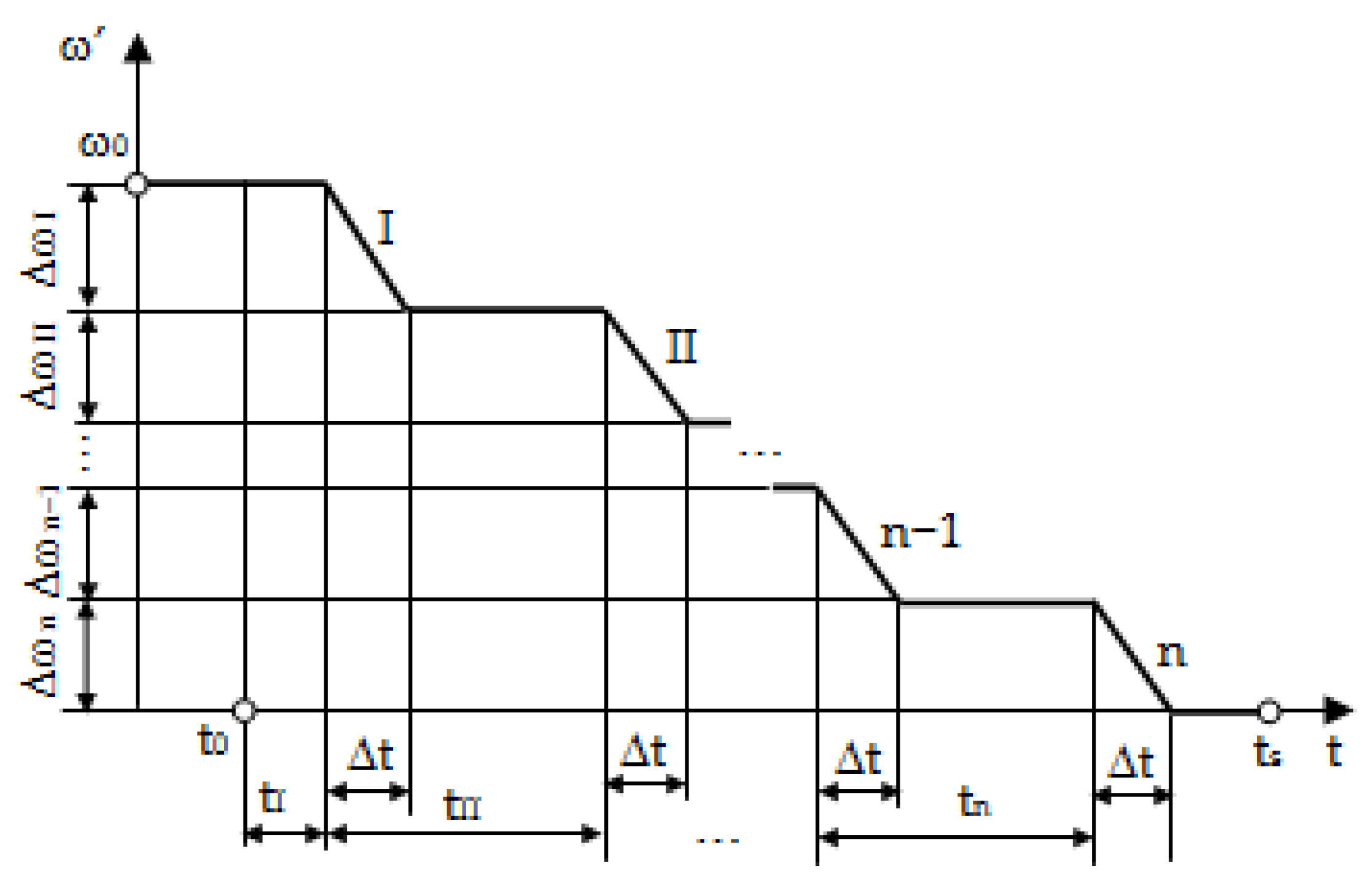
The modeling in ADAMS of the time variation law for the diurnal angle is based on the predefined STEP function, which is a run-time function with the following format/syntax [66]:

STEP (x, Begin At, Initial Function Value, End At, Final Function Value),

(10)

where x is the independent variable (in this case, time), Begin At is the initial value of independent variable at which the STEP function begins, Initial Function Value is the initial value of the step, End At is the value of the independent variable at which the STEP function ends, and Final Function Value is the final value of the step. Thus, the step-by-step tracking law for the range of movement between the morning and noon positions is defined/modeled by a summation of STEP functions (corresponding to the number of tracking steps), as follows (Figure 22):

$$\begin{array}{c}\mathrm{STEP}\left(\mathrm{t}, \left({\mathrm{t}}_0{ + \mathrm{t}}_{\mathrm{I}}\right){, \mathrm{\omega }}_0, \left({\mathrm{t}}_0{ + \mathrm{t}}_{\mathrm{I}}+\mathrm{\Delta }\mathrm{t}\right){, \mathrm{\omega }}_0{ - \mathrm{\Delta }\mathrm{\omega }}_{\mathrm{I}}\right)+\mathrm{STEP}\left(\mathrm{t}, \left({\mathrm{t}}_0{ + \mathrm{t}}_{\mathrm{I}} {+ \mathrm{t}}_{\mathrm{II}}\right), 0, \left({\mathrm{t}}_0{ + \mathrm{t}}_{\mathrm{I}}{ + \mathrm{t}}_{\mathrm{II}} +\mathrm{\Delta }\mathrm{t}\right){, - \mathrm{\Delta }\mathrm{\omega }}_{\mathrm{II}}\right) \\ + \dots + \mathrm{STEP}\left(\mathrm{t}, \left({\mathrm{t}}_0{ + \mathrm{t}}_{\mathrm{I}} {+ \mathrm{t}}_{\mathrm{II}} +\dots {+\mathrm{t}}_{\mathrm{n}}\right), 0, \left({\mathrm{t}}_0{ + \mathrm{t}}_{\mathrm{I}} {+ \mathrm{t}}_{\mathrm{II}} +\dots {+\mathrm{t}}_{\mathrm{n}} + \mathrm{\Delta }\mathrm{t}\right){, - \mathrm{\Delta }\mathrm{\omega }}_{\mathrm{n}}\right). \end{array}$$

(11)

where t₀ is the sunrise time; t_I—the start time for the first movement step, by adding to t₀; t_II—the start time for the second movement step, by adding to the start time of the first step; t_n—the start time for the last movement step, by adding to the start time of the previous step (n − 1); Δt—the duration of the movement step (to simplify the optimization process, the same duration was considered for all movement steps, no matter how large their amplitudes/sizes are); ω₀—the starting value of the diurnal angle (that corresponding to the initial/morning position, when the PV module is facing east); Δω_I—the amplitude of the first movement step; Δω_II—the amplitude of the second movement step; and Δω_n—the amplitude of the last movement step (the one that occurs before solar noon, t_s). As follows from Equation (11), with the second movement step, the value (either the initial or the final) of the current function is related to the preceding value, either the final value from the preceding function or its initial value.

Except for the parameters t₀ and Δt (which are defined by functional requirements), the other parameters involved in Equation (11) will be considered as independent design variables for the optimization process of the step-by-step tracking law. For each variable, an initial value and a variation range (minimum–maximum) have been defined.

To ensure the condition that the last movement step be performed before solar noon, a design constraint was entered into the model by the following expression:

$$\mathrm{DC}=\left({\mathrm{t}}_0{ + \mathrm{t}}_{\mathrm{I}}{ + \mathrm{t}}_{\mathrm{II}}+\dots {+ \mathrm{t}}_{\mathrm{n}}+\mathrm{\Delta }\mathrm{t}\right){ - \mathrm{t}}_{\mathrm{s}} \le 0,$$

(12)

where the meaning of the design constraint and how it is treated in ADAMS are similar to those presented in the optimization of the mechanical device of the tracking mechanism (the design constraint is satisfied/respected as long as the corresponding function remains negative or at the null limit).

Given that the number of tracking steps (n) is a design variable, defined by a predefined variation range during optimization, n ∈ [n_min, n_max], to make it possible to automatically update the number of STEP functions in Equation (11), it was chosen to use a conditional “IF” function, having the format below [66]:

IF(Function1: Function2, Function3, Function4),

(13)

where Function1 is the function/expression that ADAMS evaluates: if the value of Function1 is less than 0, IF returns Function2; if the value of Function1 is 0, IF returns Function3; and if the value of Function1 is greater than 0, IF returns Function4. As examples, the forms of Equation (11) are presented below for the cases where the range of variation of the number of movement steps is n ∈ [1, 2], Equation (14), and n ∈ [1, 3], Equation (15):

$$\mathrm{IF}\left(\begin{array}{l}\mathrm{n}-1: 0, \mathrm{STEP}\left(\mathrm{t}, \left({\mathrm{t}}_0{ + \mathrm{t}}_{\mathrm{I}}\right), {\mathrm{\omega }}_0, \left({\mathrm{t}}_0{ + \mathrm{t}}_{\mathrm{I}}+\mathrm{\Delta }\mathrm{t}\right), {\mathrm{\omega }}_0 - \mathrm{\Delta }{\mathrm{\omega }}_{\mathrm{I}}\right), \mathrm{STEP}\left(\mathrm{t}, \left({\mathrm{t}}_0{ + \mathrm{t}}_{\mathrm{I}}\right), {\mathrm{\omega }}_0, \left({\mathrm{t}}_0{ + \mathrm{t}}_{\mathrm{I}}+\mathrm{\Delta }\mathrm{t}\right), {\mathrm{\omega }}_0 - \mathrm{\Delta }{\mathrm{\omega }}_{\mathrm{I}}\right)+\\ +\mathrm{STEP}\left(\mathrm{t}, \left({\mathrm{t}}_0{ + \mathrm{t}}_{\mathrm{I}} {+ \mathrm{t}}_{\mathrm{II}}\right), 0, \left({\mathrm{t}}_0{ + \mathrm{t}}_{\mathrm{I}}{ + \mathrm{t}}_{\mathrm{II}} +\mathrm{\Delta }\mathrm{t}\right), - \mathrm{\Delta }{\mathrm{\omega }}_{\mathrm{II}}\right)\end{array}\right),$$

(14)

$$\mathrm{IF}\left(\begin{array}{l}\mathrm{n}-2: \mathrm{STEP}\left(\mathrm{t}, \left({\mathrm{t}}_0{ + \mathrm{t}}_{\mathrm{I}}\right), {\mathrm{\omega }}_0, \left({\mathrm{t}}_0{ + \mathrm{t}}_{\mathrm{I}}+\mathrm{\Delta }\mathrm{t}\right), {\mathrm{\omega }}_0 - \mathrm{\Delta }{\mathrm{\omega }}_{\mathrm{I}}\right), \mathrm{STEP}\left(\mathrm{t}, \left({\mathrm{t}}_0{ + \mathrm{t}}_{\mathrm{I}}\right), {\mathrm{\omega }}_0, \left({\mathrm{t}}_0{ + \mathrm{t}}_{\mathrm{I}}+\mathrm{\Delta }\mathrm{t}\right), {\mathrm{\omega }}_0 - \mathrm{\Delta }{\mathrm{\omega }}_{\mathrm{I}}\right)+\\ +\mathrm{STEP}\left(\mathrm{t}, \left({\mathrm{t}}_0{ + \mathrm{t}}_{\mathrm{I}} {+ \mathrm{t}}_{\mathrm{II}}\right), 0, \left({\mathrm{t}}_0{ + \mathrm{t}}_{\mathrm{I}}{ + \mathrm{t}}_{\mathrm{II}} +\mathrm{\Delta }\mathrm{t}\right), - \mathrm{\Delta }{\mathrm{\omega }}_{\mathrm{II}}\right), \mathrm{STEP}\left(\mathrm{t}, \left({\mathrm{t}}_0{ + \mathrm{t}}_{\mathrm{I}}\right), {\mathrm{\omega }}_0, \left({\mathrm{t}}_0{ + \mathrm{t}}_{\mathrm{I}}+\mathrm{\Delta }\mathrm{t}\right), {\mathrm{\omega }}_0 - \mathrm{\Delta }{\mathrm{\omega }}_{\mathrm{I}}\right)+\\ +\mathrm{STEP}\left(\mathrm{t}, \left({\mathrm{t}}_0{ + \mathrm{t}}_{\mathrm{I}} {+ \mathrm{t}}_{\mathrm{II}}\right), 0, \left({\mathrm{t}}_0{ + \mathrm{t}}_{\mathrm{I}}{ + \mathrm{t}}_{\mathrm{II}} +\mathrm{\Delta }\mathrm{t}\right), - \mathrm{\Delta }{\mathrm{\omega }}_{\mathrm{II}}\right)+ \mathrm{STEP}\left(\mathrm{t}, \left({\mathrm{t}}_0{ + \mathrm{t}}_{\mathrm{I}} {+ \mathrm{t}}_{\mathrm{II}} + {\mathrm{t}}_{\mathrm{I}\mathrm{I}\mathrm{I}}\right), 0, \left({\mathrm{t}}_0{ + \mathrm{t}}_{\mathrm{I}} {+ \mathrm{t}}_{\mathrm{II}} + {\mathrm{t}}_{\mathrm{I}\mathrm{I}\mathrm{I}} + \mathrm{\Delta }\mathrm{t}\right), - \mathrm{\Delta }{\mathrm{\omega }}_{\mathrm{III}}\right)\end{array}\right).$$

(15)

The optimization algorithm of the tracking program is that used in the optimal design of the mechanical and control devices, namely, OPTDES-GRG with the centered differentiation method. Once the values of the design variables for half of the tracking law, from sunrise to noon, have been determined, the symmetrical transposition for the afternoon interval, from noon to sunset, is made by inverting the sign of the diurnal angle. In addition to the active route of the PV system, from sunrise to sunset, the full tracking law also includes the passive route after sunset, through which the system returns to the initial position, ω₀ (from which Sun tracking will start the next day). Obviously, the PV module produces energy (E_t in Equation (4)) only on the active route, but it consumes energy (E_c in Equation (4)) to carry out the necessary movements both on the active and passive routes.

As mentioned before, an important advantage of equatorial systems is that the elevation angle (δ′) does not have to be changed during a day; in other words, the tilt angle of the module remains constant at the value determined as optimal, throughout the day.

The optimization algorithm of the tracking program was tested for several days during the year. In the following, the results obtained for one of the representative days of the year, the longest day, i.e., the summer solstice day (N = 172—21 June, sunrise/sunset time—4.26/19.74, as solar time), are presented.

From the point of view of diurnal movement, a tracking law with n = 12 steps was determined to be optimal (6 tracking steps in the morning and the same in the afternoon, symmetrical to the noon position). The angular range of the diurnal movement is 120°, meaning ω′ ∈ [+60°, −60°] (so, ω₀ = 60° in Figure 22). For the half-law from morning to noon, very close values in terms of the amplitudes of diurnal movement steps (Δω) were obtained as follows: Δω_I = 10.019°, Δω_II = 9.988°, Δω_III = 9.973°, Δω_IV = 9.977°, Δω_V = 10.028°, and Δω_VI = 10.015°. In these terms, for further simplification, the obtained values have been rounded, thus resulting in equal values for the diurnal tracking steps, Δω_I–VI = 10°, with these values being later used for the transposition of the movement law corresponding to the interval from noon to evening. The start time for the six tracking steps, as they are defined in Figure 22 and Equation (11), resulted as follows: t_I = 3.62, t_II = 0.75, t_III = 0.79, t_IV = 0.77, t_V = 0.74, and t_VI = 0.63. These relative values correspond to the following moments of time when the tracking steps are initiated (in solar time): T_I = t₀ + t_I = 7.88, T_II = T_I + t_II = 8.63, T_I = T_II + t_III = 9.42, T_IV = T_III + t_IV = 10.19, T_V = T_IV + t_V = 10.93, and T_VI = T_V + t_VI = 11.56.

From the elevation position point of view, the optimal value of the tilt angle of the PV module during the day under consideration (summer solstice) is δ′ = 22.20°, which corresponds to the solar declination angle δ = 23.45°.

Based on the so obtained values of the diurnal and elevation angles, as well as the times (as absolute values) in which the tracking steps are initiated, the tracking program for the whole day was obtained (

Table 3. Tracking program for the summer solstice day.

Movement		Diurnal			Elevation
Actuation Time|Angle		Step Initiation Time	Step Start Value	Step End Value
Tracking step no.	I	7.88	60.0°	50.0°	22.20°
	II	8.63	50.0°	40.0°
	III	9.42	40.0°	30.0°
	IV	10.19	30.0°	20.0°
	V	10.93	20.0°	10.0°
	VI	11.56	10.0°	0.0°
	VII	12.44	0.0°	−10.0°
	VIII	13.07	−10.0°	−20.0°
	IX	13.81	−20.0°	−30.0°
	X	14.59	−30.0°	−40.0°
	XI	15.37	−40.0°	−50.0°
	XII	16.12	−50.0°	−60.0°
	return	19.74	−60.0°	60.0°

). It should be mentioned that for the diurnal movement, the return route of the PV system to the initial position (for the next day), after the sunset, is also considered; in other words, the energy consumption to achieve the tracking includes the consumptions corresponding to the active and passive routes.

By transposing the numerical results from Table 3 in graphical forms, the time variation diagrams for the imposed position angles of the PV module were obtained, as shown in Figure 23, where “d” is for the diurnal movement, while “e” is for the elevation movement. These movement laws are inputs in the tracking mechanism control system model (see Figure 17), through the block Tabular Function of Time (T1). For these position angles imposed on the PV module, the corresponding strokes, i.e., linear displacements, in the two actuators (which were determined by the inverse kinematic analysis of the tracking system, according to the analysis algorithm in Figure 10) are those shown in Figure 24. Obviously, in the case of the diurnal movement actuator, the time variation law for the corresponding linear displacement (denoted by “d”) is of the step-by-step type, similar to the diurnal angle profile, while the elevation actuator remains fixed in the position that ensures the imposed/required elevation angle, δ′ = 22.20° (obviously, the linear displacement in this actuator, denoted by “e”, is constant at a zero value during the whole day under consideration). It is recalled that the linear displacements in the two actuators are related to the initial positions in the two movement subsystems (according to Figure 5a and Figure 8a), when the actuators are fully compressed.

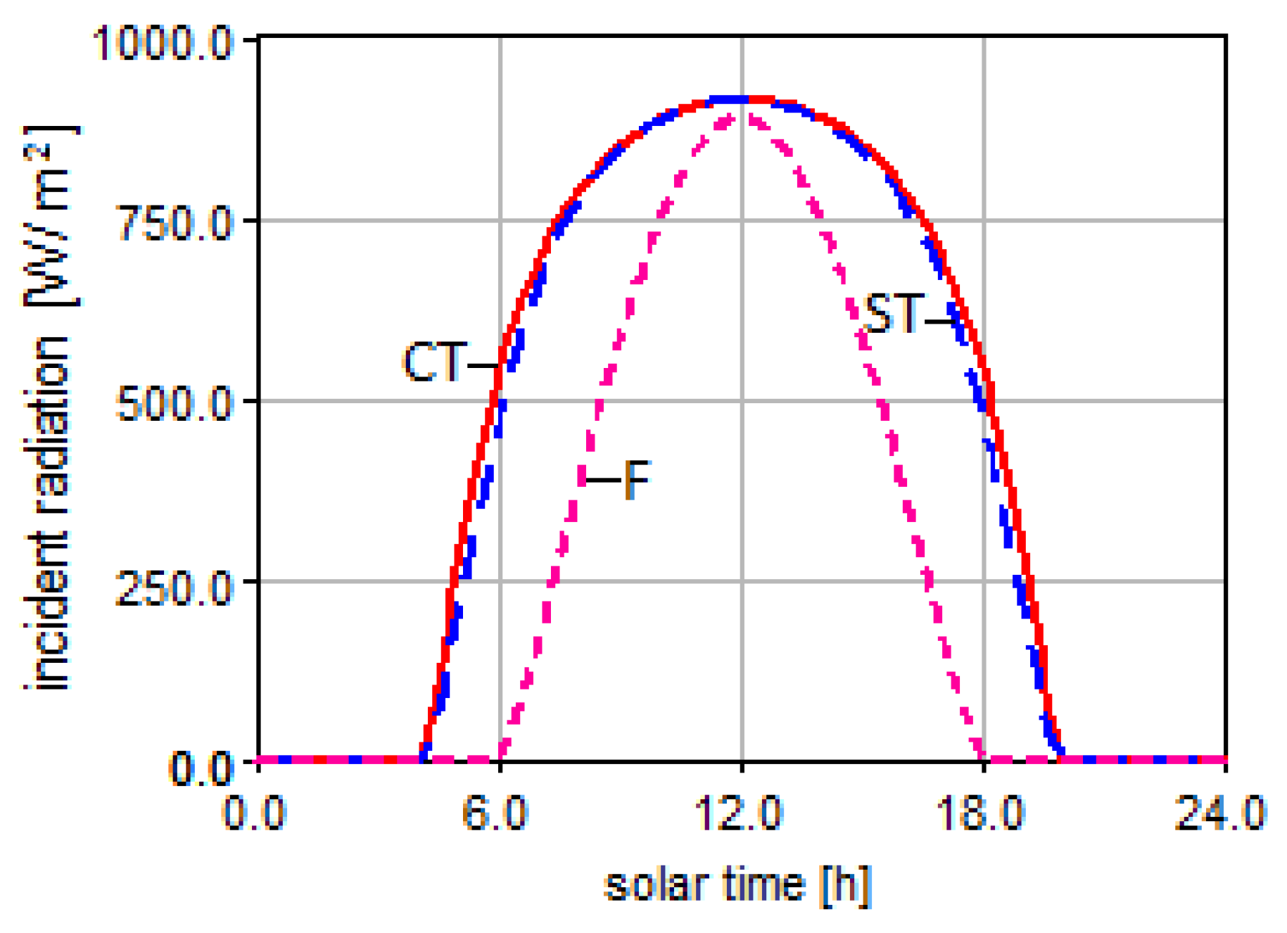
With this tracking program, based on the computation algorithm summarized by Equations (6)–(8), the incident solar radiation curves have been obtained for the following three cases (Figure 25): “ST”—PV system with step-by-step tracking (according to Table 3 and Figure 23); “F”—fixed equivalent PV system; and “CT”—continuous tracking during the entire daylight period (from sunrise to sunset), in the maximum angular range for diurnal motion, ω′ ∈ [+90°, −90°]. For the fixed system, the PV module is kept in the noon position, facing south (so, ω′ = 0), with the elevation angle having the value (obviously, constant) determined to be optimal during the year (as the average of the elevation angle values from the 365 days of the year), namely, δ′ = 45.65°. In the ideal case (from the point of view of the degree of capture of solar radiation) of continuous orientation, the obtained incident radiation curve actually coincides with the direct radiation curve (so, R_I = R_D in Equation (6)), with the angle of incidence being zero during the whole daylight period. As can be seen from Figure 25, the incident radiation curve for the step-by-step orientation (based on the proposed tracking program) is very close to that of the ideal continuous tracking case, which demonstrates the viability/usefulness of the previously presented optimal design algorithm.

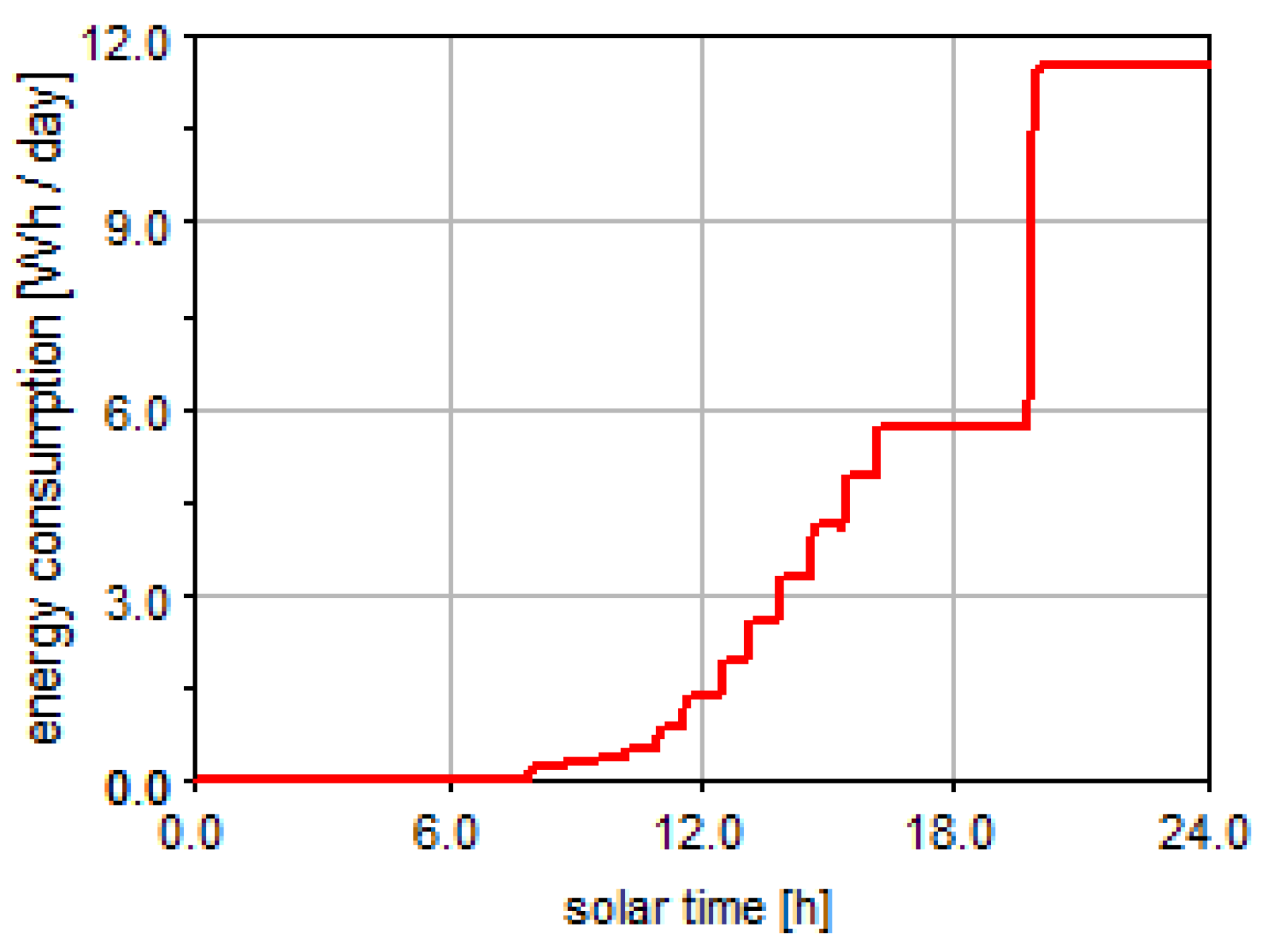
By integrating the incident radiation curves, and taking into account the active surface of the module as well as its conversion efficiency, the amounts of electric energy produced by the PV system were obtained according to Equation (5), as follows (Figure 26): E_{t_ST} = 1930.18 Wh/day, E_f = 1209.31 Wh/day, and E_{t_CT} = 2003.71 Wh/day (the notations are similar to those used in Figure 25). The amount of energy produced by the PV system with step-by-step tracking is very close to that produced in the case of continuous orientation, and substantially higher than that in the case of the fixed system.

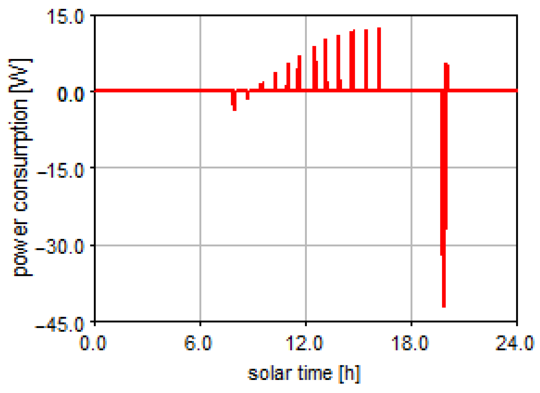
Finally, in order to evaluate the net energy gain of the PV system equipped with the proposed tracking mechanism, it was necessary to determine the amount of energy consumed to achieve the tracking. This resulted from the dynamic analysis of the mechatronic model of the tracking system (which integrates the mechanical device designed in ADAMS, Figure 2, and the control system in EASY5, Figure 17), based on Equation (9). Practically, through the co-simulation performed in ADAMS and EASY, the power consumption was obtained (Figure 27), from which later, through integration, the energy consumption was determined (Figure 28).

Thus, the energy gain of the proposed system was determined according to Equation (4), as follows:

$$\mathrm{e}=\frac{{\mathrm{E}}_{\mathrm{t}}-\left({\mathrm{E}}_{\mathrm{f}}+{\mathrm{E}}_{\mathrm{c}}\right)}{{\mathrm{E}}_{\mathrm{f}}}\cdot 100=\frac{1930.18 - \left(1209.31+ 11.53\right)}{1209.31}\cdot 100 = 58.66\%.$$

Similar simulations/computations were carried out for several representative days of the year, from all seasons, with the average value of the energy gain during the year being around 42%, which fully justifies the use of the proposed equatorial dual-axis tracking mechanism. The annual energy gain was computed as the average of the corresponding gains in 12 representative days of the year (1 per month). The representative day of a month is that day in which the value of the solar declination angle (δ) is closest to the average of the declination values for all the days of the month under consideration (δ_m). In this regard,

Table 4. Energy gain on the representative days.

Representative Day	N	δ [°]	δm [°]	e [%]
17 January	17	−20.73	−20.67	34.19
15 February	46	−12.95	−13.00	37.14
16 March	75	−2.02	−1.99	38.32
15 April	105	9.78	9.86	44.55
15 May	135	19.03	19.04	51.64
10 June	161	23.09	23.11	58.22
17 July	198	21.01	20.93	51.26
16 August	228	13.12	12.97	44.55
16 September	259	1.41	1.60	38.96
16 October	289	−10.33	−10.21	36.69
15 November	319	−19.38	−19.28	35.06
10 December	344	−23.12	−23.12	33.46

presents the representative days of the year, as well as the energy gains corresponding to these days, which have been determined in a similar way to those previously presented in detail for the summer solstice day.

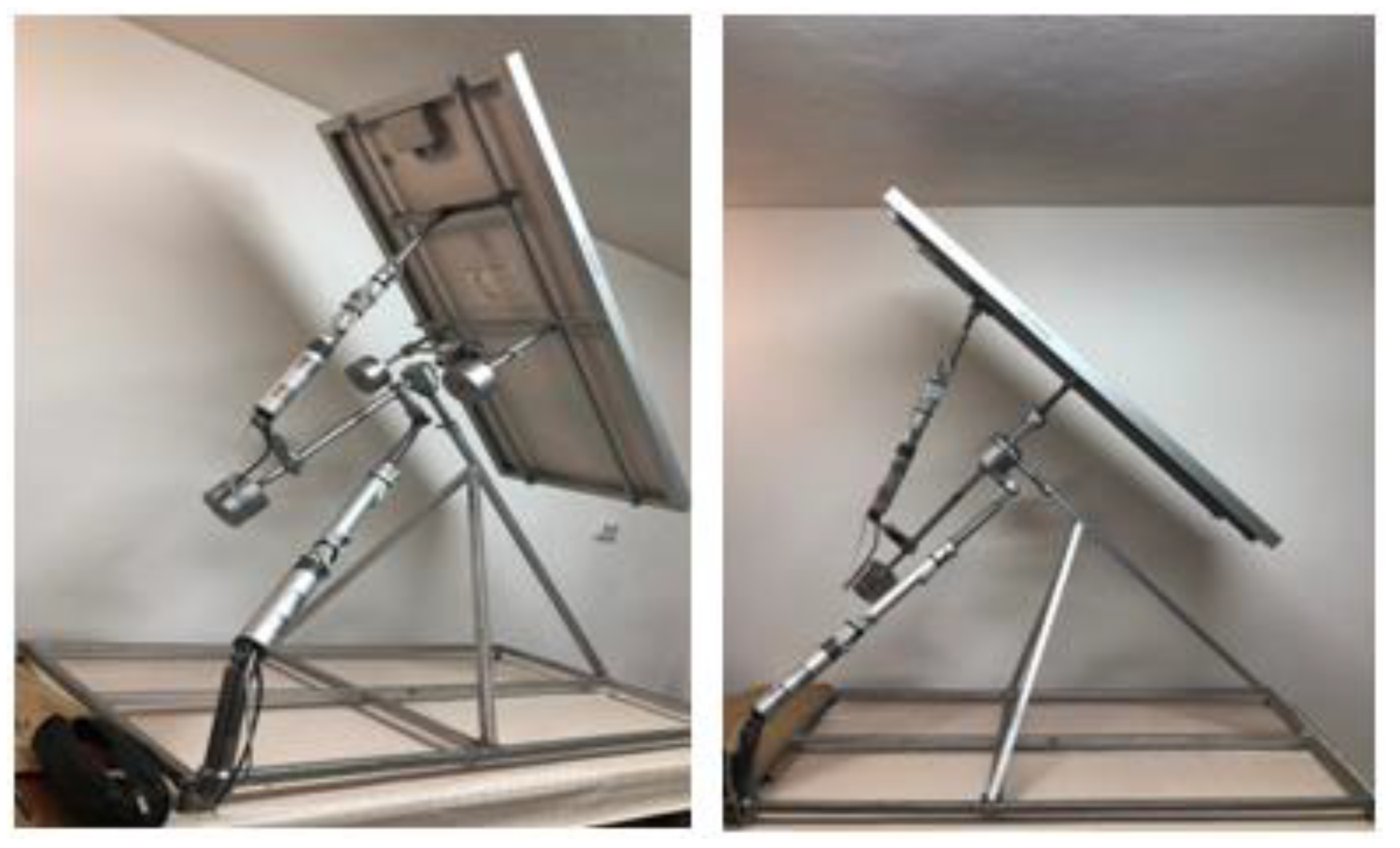
A detailed study on the energy gain throughout the year as well as on the step-by-step tracking efficiency by reporting to the ideal case of continuous tracking will be presented in a future paper. This will also aim to compare (for mutual validation purposes) the simulation results (such as those in the present work) with the results obtained by testing (in the real environment) the physical prototype of the tracking system (Figure 29), which was recently developed based on the specifications of the virtual prototype and is currently under implementation in the solar park within the Faculty of Product Design and Environment.

Although apparently the vast majority of specific aspects in the PV tracking systems are treated in sufficient detail in the literature, there are still opportunities (research perspectives) that deserve to be explored. One of these opportunities refers to the more in-depth research of adaptive tracking systems, which should be able to make tracking decisions based on real weather conditions (including the external disturbances, such as wind action) and also relying on meteorological forecasts. Another important research opportunity refers to the development of more efficient solutions and strategies to avoid the overheating of PV modules, which would lead to a dramatic decrease in their efficiency. Finally, it is necessary to deepen the research in the design of innovative combined tracking and wiper mechanisms, which additionally to their main function (that of mono-axial or bi-axial orientation, by case) should also be capable of cleaning the PV module’s surface (without the need to use a supplementary/separate actuating source), so as to maintain the conversion efficiency of the PV module as best as possible.

5. Conclusions

Based on the study depicted in this work, the following conclusions can be drawn (with reference to the proposed equatorial dual-axis tracking system and to the software tools used in the design process, including the algorithm by which the system was optimized):

-

The proposed tracking mechanism is a relatively simple one, both functionally and constructively, with beneficial effects on system maintainability and reliability;

-

The dual-axis system is very effective from the point of view of capturing solar radiation as it is capable of accurately reproducing the real movements of the Sun–Earth astronomical system and, at the same time, by the fact that the two movements are independent from each other, so the control process is significantly simplified;

-

By the way in which the two linear actuators are arranged, the necessary angular ranges for diurnal and elevation movements can be achieved without the need to use additional mechanisms for amplifying the stroke, which would have meant including additional costs;

-

The system of counterweight used to balance the mechanism allows for bringing the centers of mass of the moving structures very close to the rotation axes, which has a positive effect on the energy consumption required to carry out the necessary movements;

-

The single-loop control system based on the PID controller allows for obtaining high-stability and robust performance, which also has the effect of eliminating solar radiation losses caused by possible positioning (tracking) errors of the PV module;

-

Through the optimal design of the bi-axial tracking program, in a model where not only both specific subsystems of the mechatronic system (mechanical the control) are integrated but also the mathematical algorithm for estimating the amount of energy produced by the PV system, a significant energy gain is obtained compared to the case of the fixed equivalent system;

-

In the virtual prototype of the tracking system, various measurements can be made at any location and for any type of parameter (motion, force, and energy), including parameters that would be very difficult or even impossible to measure with the physical model, for example, due to the lack of adequate sensors or insufficient space for their installation.

As a further research direction on the tracking system proposed in this work, the evaluation of its economic efficiency, as an investment and its expected income generation, constitutes a priority. In this regard, it is intended to evaluate the energy efficiency of the tracking system correlated with cost analysis studies [67,68], by reporting the solution proposed in this work (that of a dual-axis mechanism) with the simplified versions of single-axis and fixed systems, respectively. Such a study assumes the simultaneous consideration of the electrical power generated by the PV system but also of the installation and maintenance costs (both for the mechanical structure and for the electrical and electronic components), for the purpose of determining (estimating) the payback period, in which the cost involved in ensuring the orientation of the PV module can be redeemed.

Through another future research direction, it is intended to use the proposed tracking system not only as a stand-alone system for energy production but also in larger interdisciplinary projects, such as agrivoltaic systems [69,70], which refer to various methods of combining crops with solar modules (with or without tracking). A basic requirement for such systems is that regarding the light sharing between the PV modules and the underlying crops, and here, the tracking systems can play an important role in order to find an optimal balance between energy production and plant growth. In this regard, it will also be necessary to adapt the proposed tracking system for a string-type configuration, either with individual actuation of the PV modules or with simultaneous actuation from the same motor source by using additional mechanisms to transmit movement between modules.