Commit-Level Software Change Intent Classification Using a Pre-Trained Transformer-Based Code Model

Abstract

Software evolution is driven by changes made during software development and maintenance. While source control systems effectively manage these changes at the commit level, the intent behind them are often inadequately documented, making understanding their rationale challenging. Existing commit intent classification approaches, largely reliant on commit messages, only partially capture the underlying intent, predominantly due to the messages’ inadequate content and neglect of the semantic nuances in code changes. This paper presents a novel method for extracting semantic features from commits based on modifications in the source code, where each commit is represented by one or more fine-grained conjoint code changes, e.g., file-level or hunk-level changes. To address the unstructured nature of code, the method leverages a pre-trained transformer-based code model, further trained through task-adaptive pre-training and fine-tuning on the downstream task of intent classification. This fine-tuned task-adapted pre-trained code model is then utilized to embed fine-grained conjoint changes in a commit, which are aggregated into a unified commit-level vector representation. The proposed method was evaluated using two BERT-based code models, i.e., CodeBERT and GraphCodeBERT, and various aggregation techniques on data from open-source Java software projects. The results show that the proposed method can be used to effectively extract commit embeddings as features for commit intent classification and outperform current state-of-the-art methods of code commit representation for intent categorization in terms of software maintenance activities undertaken by commits.

1. Introduction

Software changes serve as core building blocks of software evolution [1] in both the software development and maintenance phases of a software development life cycle. Throughout the development of a software system, every change made to the software aims to make a step forward towards producing and delivering a software product that meets the users’ needs [2]. In contrast, changes performed after the delivery of software, i.e., during software maintenance, are necessary to ensure the product’s continuous usefulness for the users and, ultimately, its survival [3,4,5]. For these reasons, software changes are viewed as being at the core of software engineering practices. To efficiently manage the changes made to source code during a software’s lifetime, source control systems, such as Git and SVN, have become the de facto standard in modern software engineering [6]. In such systems, the tracked changes are organized as commits. Commits are stored within a code repository of a software project and represent a snapshot of source code at a certain time in the software project’s version history.

Behind every commit in a software repository lies a reason that drove that particular set of code changes. This underlying rationale can provide insightful information for both software researchers and practitioners; however, when changes are committed to the repository, the intent of the changes is rarely properly documented [7,8]. One way to identify the intent of the undertaken changes in a commit is to manually inspect the commit by taking a closer look at, for example, the modifications to the code, the committer’s notes that can be found in the form of a commit message, software documentation, and external documentation. However, prior studies have demonstrated how labor-intensive, time-consuming, and expensive such an approach is, in addition to questionable scalability for large software projects in real-world use cases [6,9]. Furthermore, when intent identification is performed by humans for an extensive number of commits and projects, in particular retrospectively, it tends to be error-prone [7]. To address the need for automated approaches for intent identification, many researchers have attempted to construct machine-learning-based commit classification models as an alternative to resorting to manual efforts. Recent studies in the field have demonstrated that such models are adequate for the task [6,7,8,10,11,12,13,14,15,16,17].

In this context, the majority of existing research focuses on identifying the intent of the commit change in terms of the type of maintenance activity carried out in a commit. The importance given to maintenance activities mainly lies in the substantial amount of resources these activities consume; ranging from approximately 50% [18] to as much as 90% [19] of total expenses devoted to a software project. Therefore, there is significant interest in deepening the understanding of software maintenance as a crucial part of software evolution and improving software practices related to software maintenance; the previously discussed commit classification models can be of assistance to this in many ways. Firstly, by having a historical record of maintenance activities performed throughout maintenance, managers can gain a better understanding of how effectively they are planning maintenance tasks, managing maintenance expenses, and allocating available resources [11,14,15,20]. In addition to analyzing commit intents retrospectively, commit intent information can assist managers in making decisions regarding planning future activities, allocating resources, assessing the project’s health, managing technical debt, etc., all of which can collectively make maintenance more efficient, minimize costs and efforts, and preempt potential issues [11,14,15,20]. For example, by having an insight into resources needed for a type of maintenance activity in the past, it is easier to plan for future maintenance needs [6]. As another example, by obtaining current data on the number of commits associated with each type of maintenance activity, managers can reallocate resources accordingly or investigate the underlying causes of unexpected increases in commits related to a specific activity type [11]. The classifications produced by an accurate commit intent classification model can also be used to identify anomalies in software evolution, such as verifying if the unplanned type of activity is carried out. For instance, in projects presumed to be in the feature freeze phase, the work on adding new features should not be undertaken [7,21]. Additionally, many research endeavors benefit from commit intent information to support empirical research in investigating software changes, evolution, and maintenance [8] or to improve the maintenance processes for software practice. As an example, some researchers aim to focus only on a specific type of maintenance activity [6], for which the commit classification models can be utilized as a starting point. Similarly, they can be helpful to direct a developer to a specific type of software change [6]. Commit intent information can also be used to build developer’s maintenance profiles [22], to prioritize code reviews [8], and to aid in the early detection of software projects with degrading software quality [7] or lacking in proper maintenance support [23]. Hence, there is a need to have robust and reliable automated approaches for commit intent classification, as their ability to determine the intent of a change accurately has a direct impact on these aforementioned use cases and applications.

While existing approaches to commit intent classification have been shown to be somewhat successful at the task, there are still many open challenges to address associated with the complex and challenging nature of software changes and the subtle distinctions between different intent types. Models with high accuracy, robustness, and reliability are still lacking. Existing models that base their classification entirely on the content of a commit message are likely to perform poorly in cases where the messages are not present, incomplete, or of low quality [5,7,8]. Additionally, these models do not consider the changes made to the source code at all, even though the actual changes are in the code itself. The approaches that leverage the actual changes in the source code, characterized by its unstructured nature, mainly rely on code change metrics derived from the code, capturing size-related characteristics of the code or patterns identified by code change distiller tools. However, the potential benefits of using the semantics of the code for commit intent classification have yet to be fully explored [24].

To address this research gap, this work is the first to present an approach to commit-level software change intent classification into software maintenance activities based on embedding code changes using a pre-trained transformer-based code model. To tackle the unstructured nature of source code, we build upon the recent advancements in code representation learning models by simultaneously exploiting the representation capabilities of these models to capture code semantics. Thus, our proposed method is based on a pre-trained code model that is further trained using task-adaptive pre-training and fine-tuned for the task of classifying code changes based on the maintenance activities performed in those changes. The resulting model is then employed as a semantic embedding extractor, i.e., to encode fine-grained conjoint code changes, e.g., file-level or hunk-level changes, represented as additions and deletions of code lines, as code change embeddings. Finally, using a chosen aggregation technique, code change embeddings, representing fine-grained conjoint changes performed by a commit operation, are aggregated into a unified commit-level embedding.

This research aims to investigate whether the proposed method is effective when used for commit intent classification and how it compares to the current state of the art (SOTA). To achieve this, we evaluated the proposed method using two BERT-based code models, i.e., CodeBERT and GraphCodeBERT. These two code models were selected based on existing studies indicating their success in capturing code syntax and semantics, making them suitable for tasks requiring source code understanding [25,26,27,28,29,30,31,32]. To further train the pre-trained models of CodeBERT and GraphCodeBERT in a self-supervised manner, i.e., to perform task-adaptive pre-training, we constructed a dataset of more than 45,000 files affected by commit operations. To fine-tune the resulting models and build supervised machine-learning-based models for commit intent classification, we used an existing dataset of 935 commits from eleven open-source Java software projects labeled with respective intent categories in terms of maintenance activities performed in commits. For commit intent classification, commit-level embeddings obtained with the proposed method were used as inputs. Additionally, code-based commit representation features from prior studies were also considered as inputs. The output of the classification is the type of maintenance activity that was performed in a commit. The experimental results show that the build classification models based on the proposed method can accurately classify commits, capable of outperforming the SOTA. Despite this, several potential future research directions are highlighted.

In summary, this research paper makes several contributions to the field:

(1)

We propose a novel method for extracting semantic features of code changes in order to represent a commit as a vector embedding for commit intent classification into software maintenance activities.

(2)

We provide an ablation study and in-depth analyses demonstrating the effectiveness of the proposed method and its steps when used for commit intent classification into software maintenance activities.

(3)

We provide empirical evaluations of commit intent classification performance when using the proposed method compared to the existing methods of code-based commit representations for intent categorization.

The rest of this paper is organized as follows. Section 2 gives an overview of related work on commit classification and the usage of pre-trained models for code-related tasks. Section 3 introduces background knowledge relevant to our work, including the notions of commit-level software changes, commit intent classification, intent-based categorization of software maintenance activities, and transformer-based models for programming languages. Section 4 details the semantic commit feature extraction method proposed in this work. Section 5 presents the experimental setup, while Section 6 reports and discusses the obtained experimental results. Section 7 discusses threats to construct, internal, external, and conclusion validity. Section 8 concludes the paper by summarizing our findings and highlighting future research directions.

2. Related Work

2.1. Commit Classification

With the widespread adoption of source control in software development, commits emerged as a valuable unit of analysis for improving understanding of software changes, collaborative development, and software evolution [33,34,35,36]. In addition, the classification of commits was found to be beneficial for various software-engineering-related tasks, including detecting security-relevant commits [37,38], predicting the defect-proneness of commits [39,40], and demystifying the intent behind commits [6,7,8,10,11,12,13,14,15,16,17]. To tackle such challenges, the research community has extensively leveraged data associated with commits, namely, the committed code [6,7,8,11,14,37,38,41] and data from commit logs, such as commit messages [10,12,13,16,17].

In early attempts to construct commit intent classification models, researchers mainly relied on word frequency analysis with text normalization on commit messages to extract keywords indicative of maintenance categories [10]. Also utilizing commit messages as a basis for classification, several researchers employed models based on word embedding methods, notably Word2Vec [16] and various variants of BERT [12,13,17]. Our work is related to recent advances in commit intent classification, particularly those that base classification on the commit’s source code.

Levin and Yehudai [11] proposed a set of 48 code change metrics as defined by the taxonomy proposed by Fluri [42], each representing a meaningful action performed by developers. The set of metrics encompasses changes made to both the body and declaration parts of classes, methods, etc. Some examples of metrics include statement insertion/deletion and object state addition/deletion for the former, and method overridability addition/deletion and attribute modifiability addition/deletion for the latter. The authors combined the change metrics obtained using the ChangeDistiller tool with a set of 20 indicative keywords extracted from commit messages to build compound commit classification models. The approach was evaluated on a dataset the authors created using commits from GitHub repositories of eleven Java software projects. The authors manually labeled 1151 commits as corrective, adaptive, or perfective following the classification scheme suggested by Swanson [20] with the help of the committed code snippets, commit messages provided by the developer performing the changes, and information from issues tracked in the projects’ issue-tracking system.

Meqdadi et al. [6] proposed a binary commit classification model based on eight code change metrics that count the number of changed code lines, comment lines, include statements, new statements, enum statements, hunks, methods, and files. The study was performed on a manually curated dataset of 70,226 adaptive and non-adaptive commits from six C++ software projects, which the authors created themselves by inspecting commit messages.

Hönel et al. [7] proposed 20 size-based code change metrics, e.g., the number of added files, deleted, renamed, and modified files. Each of them was presented in two variations. The first variation featured unique code that only affected functionalities (i.e., code without considering whitespace, comments, and code clones). The second included all code. Two other metrics representing ratios between the size-based code change variations on the level of affected files and on the level of affected lines were proposed as well. The study was conducted on the existing dataset of Levin and Yehudai [11] with proposed code change metrics extracted from the source code using the Git Density tool. Furthermore, the authors also investigated the metrics from the perspective of considering code change metric values from preceding commits.

Ghadhab et al. [14] proposed 23 refactoring code change metrics, e.g., the presence of the extract method, move method, and rename variable operation, gathered from the code using the RefactoringMiner tool. In addition, they proposed one bug-fixing code change metric, i.e., the presence of a bug-fixing pattern, gathered using the FixMiner tool. Together with independent variables already proposed by Levin and Yehudai [11] and a fine-tuned DistilBERT for encoding commit messages, the authors assessed the performance of the proposed approach on a dataset of 1793 commits. The dataset was created from three existing datasets; labeled instances of the data of Levin and Yehudai [11], single-labeled instances from data of Mauczka et al. [43], and unlabeled instances from data of AlOmar et al. [44], which the authors labeled manually based on the content of the commit messages.

Mariano et al. [15] proposed three code change metrics, i.e., the number of added lines, deleted lines, and changed files, extracted from the source code using the GitHub GraphQL API. The authors evaluated the proposed approach using the existing dataset of Levin and Yehudai [11].

Meng et al. [8] proposed a graph representation of commits in which changed entities in a commit were represented as nodes in the graph and their relationships (i.e., dependencies recognized using static program analysis) as edges, while other characteristics were encoded as attributes of the graph’s nodes and edges. The proposed approach identified a set of relevant nodes in each graph and created the graph’s vector representation that served as input to a convolutional neural network. The approach was evaluated on a dataset of 7414 commits from five Java software projects that the authors built based on category labels defined and assigned to commits in an issue-tracking system by developers of the subject software projects. In contrast to the aforementioned related work, the authors here used their own label classification scheme; however, they claim it can be mapped directly to the one suggested by Swanson [20].

A concise overview of relevant related work that has proposed the use of features obtained from the commits’ source code is presented in

Table 1. Overview of related work utilizing features extracted from the source code for commit-level software change intent classification into software maintenance activities.

Authors	Novel Independent Variables	Dependent Variables	Dataset	Best Model Performance
Levin and Yehudai [11]	48 code change metrics following Fluri’s taxonomy [42] extracted from commits using the ChangeDistiller tool	Corrective, adaptive, and perfective labels following Swanson’s classification scheme [20]	1151 manually labeled instances sampled from commit histories of eleven open-source Java projects [11]	$Accurac{y}_{code,DT}=0.54$ $Kapp{a}_{code,DT}=0.27$ $Accurac{y}_{hybrid,DT}=0.77$ $Kapp{a}_{hybrid,DT}=0.64$
Meqdadi et al. [6]	Eight proposed code change metrics extracted from commits using a custom tool	Adaptive and non-adaptive labels following Swanson’s classification scheme [20]	70,226 manually labeled instances sampled from commit histories of six open-source C++ software projects [6,9]	$Accurac{y}_{code,DT/P}=0.65$ $F-scor{e}_{code,DT/P}=0.24$
Hönel et al. [7]	22 proposed code change metrics extracted from commits using the Git Density tool	Corrective, adaptive, and perfective labels following Swanson’s classification scheme [20]	1150 manually labeled instances sampled from commit histories of eleven open-source Java projects [11]	$Accurac{y}_{code,DT}=0.55$ $Kapp{a}_{code,DT}=0.27$ $Accurac{y}_{hybrid,DT}=0.89$ $Kapp{a}_{hybrid,DT}=0.83$
Ghadhab et al. [14]	24 proposed code change metrics extracted from commits using the RefactoringMiner tool and FixMiner tool	Corrective, adaptive, and perfective labels following Swanson’s classification scheme [20]	1793 instances sampled and semi-manually labeled from three existing datasets [11,43,44], including commits from 109 open-source Java projects [14]	$Accurac{y}_{hybrid,NN}=0.8$ $F-scor{e}_{hybrid,NN}=0.8$
Mariano et al. [15]	Three proposed code change metrics extracted from commits using the GitHub GraphQL API	Corrective, adaptive, and perfective labels following Swanson’s classification scheme [20]	1151 manually labeled instances sampled from commit histories of eleven open-source Java projects [11]	$Accurac{y}_{code,DT}=0.49$ $Kapp{a}_{code,DT}=0.19$ $Accurac{y}_{hybrid,DT}=0.77$ $Kapp{a}_{hybrid,DT}=0.64$
Meng et al. [8]	Node and edge embeddings in the change dependency graph, constructed from commits using tools ChangeDistiller, InterPart, WALA, RefactoringMiner, and a custom tool	Bug fixes, functionality additions, and other labels that can be mapped to Swanson’s classification scheme (corrective, adaptive, and perfective, respectively) [20]	7414 issue-tracking-system-based labeled instances sampled from commit history of five open-source Java software projects [8]	$F-scor{e}_{code,NN}=0.55$

DT = decision-tree-based classifier, P = probabilistic classifier, NN = neural network classifier.

. It should be noted that for each study, only proposed novel independent variables extracted from the source code (i.e., not other data sources) that were not previously proposed by others are provided in the table. This, however, means that in the studies, the authors might have combined their proposed features with the ones already proposed by others with the aim of experimenting and achieving better overall performances. Regarding classification performances, the highest evaluation metric scores achieved in cross-project settings for models based only on features extracted from code and hybrid models based on all available features (may include features extracted from other data sources than code, e.g., commit message) are reported. The classifiers used for the best-performing classification models are reported as well. As many different classifiers were employed for the task, we only report the best-fitting high-level category that the classifier belongs to, distinguishing six groups as follows: decision-tree-based, rule-based, probabilistic, support vector machines, instance-based, and neural network classifiers [45].

In addition to the reported related work, a more comprehensive overview may be found in a recently conducted systematic literature review on supervised-learning-based commit classification models into maintenance activities [5]. Our research builds on these previous efforts to represent software commits based on source code changes carried out in commits. One key difference distinguishing our work from the existing one is that no one has attempted to employ code-representation-learning models to tackle the challenge.

2.2. Pre-Trained Models in Code-Related Tasks

Due to pre-trained code-representation-learning models demonstrating good performance in code-related tasks without requiring enormous data quantities, such models have been employed across a wide variety of tasks within the domain of software engineering. Pan et al. [25] encoded Java source code files using a pre-trained CodeBERT model to aid software defect prediction. Kovačević et al. [46] conducted experiments with the Code2Vec, Code2Seq, and CuBERT models to represent Java methods or classes as code embeddings, facilitating machine-learning-based detection of two code smells, i.e., long method and god class, while Ma et al. [26] leveraged the CodeT5, CodeGPT, and CodeBERT models to detect the feature envy code smell. To compare software systems, Karakatič et al. [47] utilized a pre-trained Code2Vec model to embed Java methods. The work of Fatima et al. [27] employed the CodeBERT model to represent Java test cases, assisting in the prediction of flaky (i.e., non-deterministic) test cases. The CodeBERT model was also used by Zeng et al. [28] in order to represent C functions, aiding in detecting vulnerabilities at the function level. Mashhadi and Hemmati [29] used the CodeBERT model to represent single-line Java statements, enabling automated bug repair, while Huang et al. [48] experimented with CodeBERT and GraphCodeBERT to encode single- and multi-line segments of C code for automated repair of security vulnerabilities. The pre-trained CodeBERT model was also utilized to embed code changes to help predict the commit’s defectiveness [30] and identify silent vulnerability fixes [31]. Our research closely relates to these recent attempts to employ pre-trained code models to tackle software engineering challenges. In an effort to add to the body of knowledge, our research examines the suitability and effectiveness of code models within the specific problem domain of commit intent classification.

3. Background

3.1. Commit-Level Software Changes

A commit refers to a set of code changes a developer makes to the codebase that are tracked together as a single unit of change within a software project’s repository. Given a project’s version history containing a number of commits, which can be defined formally as

$$H=\{(c_1,t_1),(c_2,t_2),(c_3,t_3),\dots \}$$

(1)

a specific commit randomly selected from the history $c_i\in H$ represents a snapshot of the codebase at a given time $t_i$ in the project’s history. Each commit starts from the existing state of the codebase and makes modifications based on the required changes’ intent; hence, the changes introduced in a commit can be defined as the differences between the preceding and current states of the codebase $\mathit{Diff}(c_{i-1},c_i)$, where each change to the code can be thought of as either an addition of a code line or a deletion of a code line. Note that a modification of a code line effectively combines both an addition and a deletion. Accordingly, given a commit $c_i$, we may formalize it as a set of changed lines of code distributed across one or more affected files by a commit in the codebase as

$$c_i=\{({\mathit{add}}_f,{\mathit{del}}_f):{\mathit{add}}_f\in {\mathit{Diff}}_{\mathit{f}}(c_{i-1},c_i),{\mathit{del}}_f\in {\mathit{Diff}}_{\mathit{f}}(c_{i-1},c_i),\forall f\in [1,N]\}$$

(2)

where $ad{d}_f$ and $de{l}_f$ represent added and deleted lines of code in a file f, respectively, with $f\in [1,N]$ and N representing the total number of affected files by a commit operation. In the context of Git source control, changes spread across files are organized into hunks, i.e., contiguous blocks of code changes within a file. Thus, a commit can be formalized as a set of changed lines of code distributed across one or more hunks as

$$c_i=\{({\mathit{add}}_h,{\mathit{del}}_h):{\mathit{add}}_h\in {\mathit{Diff}}_{\mathit{f},\mathit{h}}(c_{i-1},c_i),{\mathit{del}}_h\in {\mathit{Diff}}_{\mathit{f},\mathit{h}}(c_{i-1},c_i),\forall f\in [1,N],\forall h\in [1,M]\}$$

(3)

where $ad{d}_h$ and $de{l}_h$ represent the lines of code added to and deleted from a hunk h, respectively, with $f\in [1,N]$ and N representing the total number of affected files by a commit operation, and $h\in [1,M]$ and M representing the total number of hunks within a file f.

3.2. Commit Intent Classification

Commit intent classification models are supervised-learning-based models that use labeled data to learn how to predict the intent of a commit, i.e., dependent variable, based on the data associated with the commit, i.e., independent variables [24]. Formally, the problem of commit intent classification can be formulated as follows. A set of labeled commits C can be defined as

$$C=\{(x_j,y_j):x_j=\langle x_{j,1},\dots ,x_{j,d}\rangle ,y_j\in \{y_1,\dots ,y_k\},\forall j\in [1,m]\}$$

(4)

where every commit instance $c_j$ from the set C is presented as a pair of $(x_j,y_j)$, with $j\in [1,m]$ and m representing the total number of labeled instances. The first part of the pair is a feature vector $\langle x_{j,1},\dots ,x_{j,d}\rangle$ that describes the commit. The feature vector has d dimensions, with each dimension of $x_j$ representing a certain feature. Considering the context of commit intent classification, features can be extracted from a variety of commit artifacts, including commit messages, source code, commit metadata, and data from external systems, such as issue tracking tools (e.g., Jira) and software quality tools (e.g., SonarQube) [5]. The second part of the pair is a label that represents the intent of the commit. The commit’s label $y_j$ is one of a predefined set of class labels $\{y_1,\dots ,y_k\}$, with k representing the total number of classes. Class labels are categories of maintenance activities, which can be either binary (two categories) or multi-class (multiple categories), following a specific intent-based categorization scheme of software maintenance activities, such as the one introduced by Swanson [20], which is most commonly used [5]. Finally, given such a labeled set C, we aim to train a model M, defined formally as

$$M:x_j\to y_j$$

(5)

where model M can predict the intent class $y_j$ of a commit $c_j$ given its feature vector $x_j$ in a way that $M\left(x_j\right)$ is a good enough prediction of the class $y_j$. The trained model M can then be used to classify new, unseen commits into their respective classes.

3.3. Intent-Based Categorization of Software Maintenance Activities

Considering what was intended to be achieved when performing maintenance activities, Swanson [20] discussed the three types of maintenance activities carried out during software maintenance: corrective maintenance, which is performed to correct functional and non-functional faults; adaptive maintenance, which is performed in response to changes in the environment and requirements; and perfective maintenance, which is performed to improve software performance and quality attributes [20,49]. According to Lientz et al. [50], 60.3% of maintenance tasks are perfective, 18.2% adaptive, and only 17.4% corrective. A follow-up study by Schach et al. [51] observed that corrective tasks are more prevalent (56.7%), while fewer tasks are perfective (39%) and adaptive (2.2%) in their nature. Figure 1 illustrates the three maintenance activities performed with a commit operation on real-world software.

3.4. Transformer-Based Models for Programming Languages

The advent of transformers, a neural network architecture initially proposed by Vaswani et al. [52], has revolutionized the field of natural language processing. Transformers represent a subset of deep learning models that introduced self-attention mechanisms and positional encodings to natural language modeling. By enabling parallel processing, thereby enhancing scalability for working with large data, transformer models addressed some key challenges associated with previously utilized recurrent neural networks. From a high-level overview of the architecture of transformers, they traditionally consist of two main parts, i.e., the encoder and the decoder. The former processes the input sequence with the aim of understanding it, while the latter aims to generate the target output based on that understanding [52]. Transformer-based models have significantly improved the performance of the SOTA in a wide range of natural language processing tasks, e.g., text classification, machine translation, text generation, sentiment analysis, question answering, and text summarization, across various domains. In the domain of software engineering, transformer models have demonstrated efficiency in understanding and generating not only human language but also programming code. Several models specifically designed for programming languages that leverage the power of transformers to encapsulate syntactic structures and the semantics of code by training on vast amounts of source code examples have been proposed. Notable representatives of such code models are CodeBERT [53], GraphCodeBERT [54], CuBERT [55], CodeT5 [56], and Codex [57].

CodeBERT and GraphCodeBERT

CodeBERT is an encoder-only transformer-based model proposed by Feng et al. [53]. It is a language model specifically designed to support understanding and generation tasks related to programming languages. The model is able to produce general-purpose contextual representations that encapsulate the syntactic and semantic patterns inherent in programming code by pre-training the model on a large and diverse corpus of both uni-modal and bi-modal data. The former refers to inputs in terms of source code snippets from various software projects and programming languages, while the latter refers to paired inputs of code snippets and their natural language documentation [53]. GraphCodeBERT is an enhancement of CodeBERT proposed by Guo et al. [54] that additionally encapsulates the inherent structure of programming code by including the data flow of code in the pre-training of code representations, which encodes the dependency relations between variables and can additionally benefit the code-understanding process.

Both CodeBERT and GraphCodeBERT use a multi-layer transformer-based neural architecture, following the BERT (Bidirectional Encoder Representations from Transformers) architecture; more specifically, they are based on the architecture of RoBERTa [53,54]. In CodeBERT, each input to the model is represented as a sequence of two distinct subsequences of tokens as $\left[\mathit{CLS}\right],t_{n{l}_1},\dots ,t_{n{l}_k},\left[\mathit{SEP}\right],t_{p{l}_1},\dots ,t_{p{l}_l},\left[\mathit{SEP}\right]$, where $t_{n{l}_k}$ and $t_{p{l}_l}$ represent tokens of two different subsequences, corresponding to natural language inputs, i.e., words, and programming language inputs, i.e., code, respectively, $\left[\mathit{CLS}\right]$ represents a special classification token at the beginning, and $\left[\mathit{SEP}\right]$ represents a special separation token that separates the two subsequences or signifies the end of the sequence [53]. In GraphCodeBERT, the input to the model is extended with an additional variable subsequence as $\left[\mathit{CLS}\right],t_{n{l}_1},\dots ,t_{n{l}_k},\left[\mathit{SEP}\right],t_{p{l}_1},\dots ,t_{p{l}_l},\left[\mathit{SEP}\right],t_{v_1},\dots ,t_{v_j}$, where $t_{v_j}$ represents a token corresponding to the variable. The subsequence of variables follows the subsequence of tokens of paired natural language-programming language inputs [54]. The output of both CodeBERT and GraphCodeBERT includes the contextual vector representation of each token from the sequence and the representation of the special classification token $\left[\mathit{CLS}\right]$, which is considered as the aggregated representation of the entire sequence [53,54].

During pre-training of CodeBERT, the model is trained in an unsupervised manner on large-scale unlabeled data using a hybrid self-supervised learning objective loss combining two pre-training objectives as ${min}_{\theta }{\mathcal{L}}_{\mathrm{MLM}}\left(\theta \right)+{\mathcal{L}}_{\mathrm{RTD}}\left(\theta \right)$, where ${\mathcal{L}}_{\mathrm{MLM}}\left(\theta \right)$ is the loss of the masked language modeling (MLM) pre-training objective and ${\mathcal{L}}_{\mathrm{RTD}}$ of the replaced token detection (RTD) pre-training objective [53]. The MLM objective uses bi-modal data and masks out a percentage of the tokens from both subsequences at randomly selected positions, and the pre-training task is to predict the original tokens that are masked out given surrounding contexts. The loss function of MLM is defined as

$${\mathcal{L}}_{\mathrm{MLM}}\left(\theta \right)=\sum _{i\in m^{t_{nl}}\cup m^{t_{pl}}}-log{p}^{D_1}\left(x_i\right|{t_{nl}}^{\mathrm{masked}},{t_{pl}}^{\mathrm{masked}})$$

(6)

where $p^{D_1}$ acts as the discriminator predicting the probability of a token based on the context of masked tokens, $m^{t_{nl}}$ and $m^{t_{pl}}$ are the random set of positions of tokens for the natural language and programming language to mask, and ${t_{nl}}^{\mathrm{masked}}$ and ${t_{pl}}^{\mathrm{masked}}$ are the masked tokens at these positions [53,58]. The second pre-training objective of CodeBERT, RTD, uses both bi-modal and uni-modal data, and the pre-training task is to detect plausible alternatives of the generated masked-out tokens [53,59]. During pre-training of GraphCodeBERT, three self-supervised training objectives are used. In addition to the MLM pre-training objective, GraphCodeBERT introduces two additional structure-aware objectives, i.e., data-flow edge prediction and node alignment pre-training. The former is designed to learn representation from data flow, while the latter is designed to align variable representations between source code and data flow [54]. To keep this paper concise, we present the loss function of the MLM pre-training objective only, as it is directly relevant to this study. For additional information on other objectives, please refer to the original papers by Feng et al. [53] and Guo et al. [54].

The publicly available pre-trained CodeBERT model and pre-trained GraphCodeBERT model were pre-trained using a large-scale dataset CodeSearchNet [60], which consists of data from publicly available open-source non-fork GitHub code repositories, including 6.4 million uni-modal and 2.1 million bi-modal data points, where each data point considers source code snippets or natural language documentation, i.e., code comments, at a function-level. Pre-trained models are designed to process input sequences of a maximum of 512 tokens, including special tokens, and output 768-dimensional embeddings [53,54].

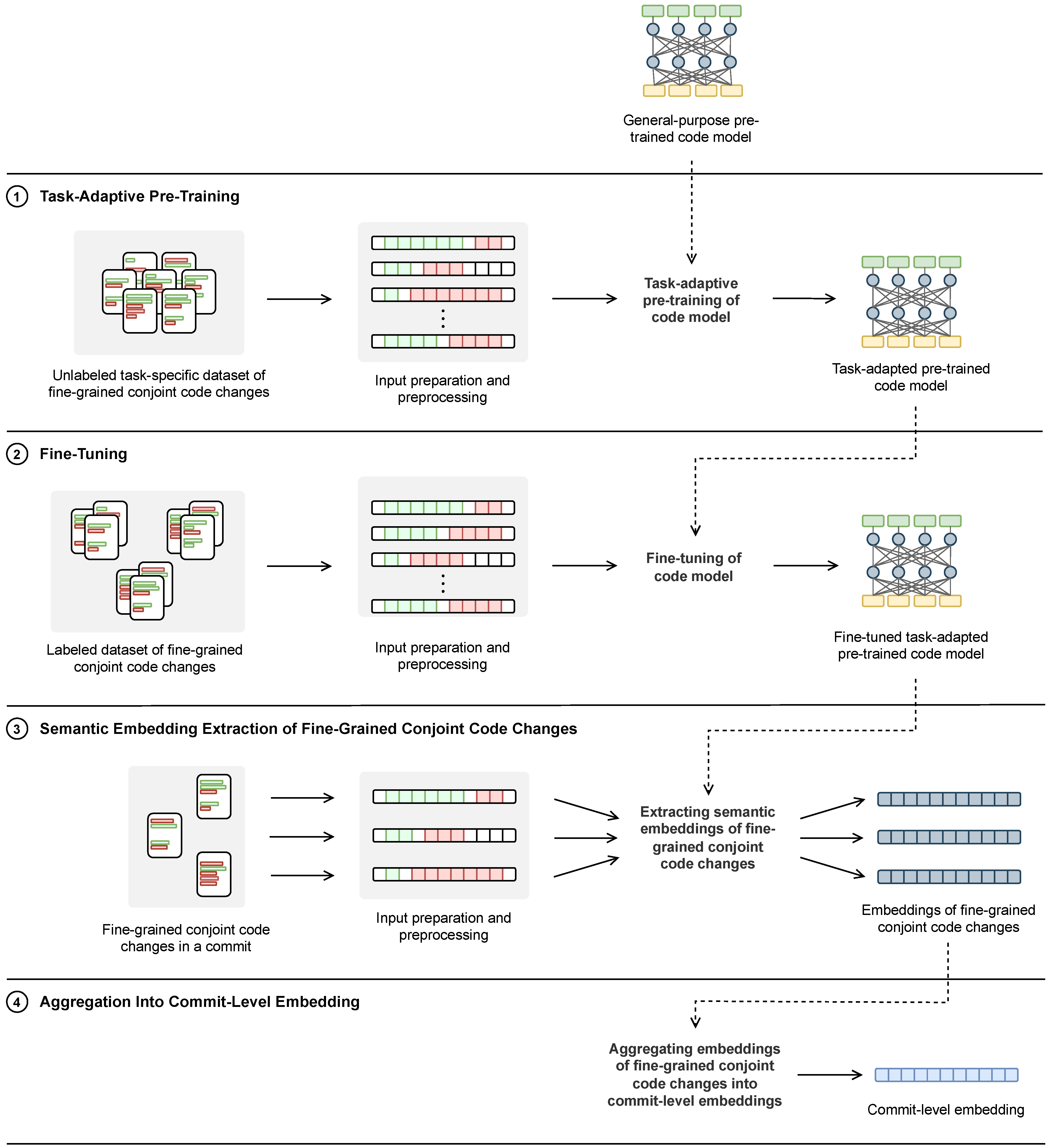
4. Proposed Semantic Commit Feature Extraction Method

From a high-level overview, the proposed method of semantic feature extraction from code changes in a commit consists of four steps: ➀ task-adaptive pre-training, ➁ fine-tuning, ➂ semantic embedding extraction of fine-grained conjoint code changes, and ➃ aggregation into commit-level embedding, as illustrated in Figure 2. In the following subsection, we outline each step of the proposed method and provide details on the implementations using CodeBERT and GraphCodeBERT, which are the models employed in this study.

4.1. Task-Adaptive Pre-Training

In the first step, a selected pre-trained code model, trained on a large and general dataset, undergoes further training as a second training phase, using a smaller, unlabeled dataset with data relevant to the given task under study. This adaptation strategy aims to refine the code model’s capabilities in performing a particular task [61]. In our case, adaptive training aims to adjust the model to reflect code changes and capture the semantics of paired inputs of added and deleted lines of code at a level of fine-grained conjoint code changes, e.g., file-level or hunk-level code changes, affected by a commit operation, which differs from the CodeBERT and GraphCodeBERT initial training on paired inputs of function-level natural language code comments and code snippets. To perform task-adaptive pre-training, a corpus closely related to the task is necessary and should ideally be drawn from the task distribution [61]. In our context, the dataset should consist of representative code additions and deletions within a single commit at the level of fine-grained conjoint changes. Such datasets can be gathered from unlabeled code repository data of software projects, based on which commit intent classification models are built, or data available in open-source code repositories. For the dataset to be usable in the training process, it needs to be prepared and preprocessed according to the selected model’s requirements, including tokenization, truncation, and padding. Specifically, for BERT-based code models, the input sequence should be constructed as detailed in Algorithm 1. This first involves converting added and deleted lines of code into tokens using the provided tokenizer of a selected code model. If these tokenized lines, along with necessary special tokens, i.e., $\left[\mathit{CLS}\right]$ at the beginning of the sequence and $\left[\mathit{SEP}\right]$ between the two subsequences and at the end, exceed the maximum input size that the model is designed to process, truncation of added and deleted tokens is required. The truncation is performed proportionally for both added and deleted code lines to ensure their balanced representation in the sequence. Alternatively, tail or head truncation can be performed. If the sequence does not meet the length requirement, it is padded with the $\left[\mathit{PAD}\right]$ special token to ensure that all input sequences are of the same length. Using such a task-specific dataset, task-adaptive pre-training starts from parameters learned through general pre-training and adjusts them through a selected self-supervised learning objective; thus building upon the existing knowledge and adapting it for the given task.

Algorithm 1 Input preparation and processing for a BERT-based code model with dynamic token length allocation, truncation, and padding

4.2. Fine-Tuning

In the second step, the task-adapted pre-trained code model from the first step undergoes further training through a process of fine-tuning for a classification task. In our case, this involves training the model on a labeled dataset specific to the task, i.e., code changes at the level of fine-grained conjoint changes, which are represented as additions and deletions of code lines, each with a known label corresponding to the intent of the change. The goal of fine-tuning is to enhance the model’s ability to accurately reflect the various intents behind code changes, represented by pairs of added and deleted code lines. To achieve this, a classification head should be added on top of the task-adapted pre-trained code model, which aids in slightly adjusting the model’s parameters to better suit the given task, based on the provided labeled dataset. Note that the same process as outlined in the previous subsection should be employed to prepare and preprocess the dataset, ensuring that the inputs are suitably formatted to meet the requirements of the selected code model.

4.3. Semantic Embedding Extraction of Fine-Grained Conjoint Code Changes

In the third step, the fine-tuned task-adapted pre-trained code model serves as a semantic embedding extractor through model inference. This entails using added and deleted lines of code of fine-grained conjoint code changes, that have been prepared and preprocessed as outlined in the previous subsections, as inputs to the model. Upon inputting this data, the embedding of the model’s $\left[\mathit{CLS}\right]$ special token is extracted. This embedding acts as a contextual aggregated vector representation of the entire input sequence, encapsulating the nuanced semantic information pertinent to the code changes.

4.4. Aggregation into Commit-Level Embedding

In the last, or fourth, step, since a commit may involve changes across several fine-grained conjoint change units, e.g., files or hunks, the embeddings of code changes affected by a specific commit operation are aggregated into a single, unified vector representation. This is achieved using a selected aggregation technique, which can involve simple dimension-wise statistical aggregations, graph-based aggregations, clustering-based aggregations, etc. The result of this step, i.e., the output of the proposed method, is a commit-level embedding representation. Such commit embeddings, derived from source code changes, can subsequently be used for a downstream task. For instance, a classifier utilizing these commit embeddings can be trained using a labeled dataset to categorize commits according to their intents. This could be, for example, based on the type of maintenance activity performed within a commit, in order to perform commit intent classification.

5. Experiments

5.1. Research Questions

With this research, our objective is to investigate and provide answers to two research questions (RQs), formulated as follows, alongside the rationales behind them:

• RQ1 How effective is the proposed method when used for commit intent classification?
  This question aims to empirically assess the effectiveness of the proposed semantic commit feature extraction method for commit intent classification. By focusing on classification performance, this evaluation aims to determine the resulting model’s ability to accurately distinguish between various types of intents behind commit-level software changes. Such an assessment is crucial as it directly relates to the practical applicability and relevance of the method in the field of software engineering.
• RQ2 How does the proposed method compare to the SOTA when used for commit intent classification?
  This question aims to benchmark the proposed method against the current SOTA in commit intent classification. By conducting this comparative analysis, the research aims to position the proposed method within the broader context of commit intent classification.

5.2. Datasets

To address the research questions, several experiments were conducted on the dataset made available by Ghadhab et al. [14], which was originally prepared by Levin and Yehudai [11]. The dataset used in the experiments consists of 935 commits from eleven open-source software projects based on Java, with manually annotated labels of commit intents in terms of the three software maintenance activities. Out of all commits, 49.4%, 26.1%, and 24.5%, are corrective, adaptive, and perfective, respectively. More detailed commit-level characteristics of the dataset used in our experiments are presented in

Table 2. Commit-level characteristics of the dataset used in the experiments.

			No. Commits
#	Software Project	Repository	Total	Corrective	Adaptive	Perfective
P1	Apache Camel	github.com/apache/camel  †	90	38 (42.2%)	21 (23.3%)	31 (34.5%)
P2	Apache HBase	github.com/apache/hbase †	97	59 (60.8%)	22 (22.7%)	16 (16.5%)
P3	Drools	github.com/kiegroup/drools †	103	60 (58.2%)	28 (27.2%)	15 (14.6%)
P4	Elasticsearch	github.com/elastic/elasticsearch †	67	28 (41.8%)	24 (35.8%)	15 (22.4%)
P5	Hadoop	github.com/apache/hadoop †	99	53 (53.5%)	26 (26.3%)	20 (20.2%)
P6	IntelliJ IDEA Community	github.com/JetBrains/intellij-community †	92	49 (53.3%)	21 (22.8%)	22 (23.9%)
P7	Kotlin	github.com/JetBrains/kotlin †	82	34 (41.5%)	15 (18.3%)	33 (40.2%)
P8	OrientDB	github.com/orientechnologies/orientdb †	96	57 (59.3%)	21 (21.9%)	18 (18.8%)
P9	Restlet Framework	github.com/restlet/restlet-framework-java †	86	41 (47.7%)	23 (26.7%)	22 (25.6%)
P10	RxJava	github.com/ReactiveX/RxJava †	61	19 (31.2%)	21 (34.4%)	21 (34.4%)
P11	Spring Framework	github.com/spring-projects/spring-framework †	62	24 (38.7%)	22 (35.5%)	16 (25.8%)
	Overall		935	462 (49.4%)	244 (26.1%)	229 (24.5%)

^† Accessed on 1 December 2023.

.

As the original dataset only contains a commit message and label for each commit, we had to extend the dataset with additional data related to fine-grained conjoint code changes to be able to use the proposed method on the dataset. In the experiments, we considered one fine-grained conjoint code change unit, i.e., file-level code changes. The steps taken to prepare and preprocess the data to obtain the extended dataset used in the experiments are presented in Algorithm 2. First, we cloned each software project’s repository to a local directory. For each labeled commit for that project, we retrieved the source code of that commit and extracted the differences in the source code between the current working directory of a commit and the preceding commit. For each file affected by the commit operation that corresponded to the Java programming language, we obtained the differences in code lines. It should be noted that different algorithms in the Git diff utility produce unequal results [62]. We used the Myers algorithm, which is used as the default in Git. We parsed the obtained difference in each file to obtain hunks with modified lines of code of a commit compared to the preceding commit by simultaneously determining whether a line was an addition or a deletion. Each modified code line was preprocessed in order to remove code comments and whitespaces, i.e., indentations and empty lines. Thus, the resulting code lines only represent the actual meaningful changes to the code itself without considering the natural language documentation in the code and code layout or formatting. Each file was assigned the same label as the commit they were part of. The resulting extended dataset contains file-level detailed information on the changes in the source code of each commit from the original dataset. Altogether, the extended dataset consists of 4513 files that were affected by a commit operation across 935 commits in eleven software projects. Across all projects, the median was two files (IQR = 3.00) were affected by a single commit, and, the median in a single file was eight lines of code (IQR = 20.00) were modified, i.e., either added or deleted. More detailed file-level characteristics of the dataset used in the experiments are available in Appendix A in

Table A1. File-level characteristics of the extended dataset used in the experiments.

		No. Affected Files Per Commit							No. Added and Deleted Lines Per File
#	Software Project	Med	IQR	Avg	Std	Min	Max		Med	IQR	Avg	Std	Min	Max
P1	Apache Camel	2.50	4.00	6.42	15.89	1.00	135.00		7.00	13.00	16.03	26.75	1.00	254.00
P2	Apache HBase	2.00	2.00	3.39	4.33	1.00	23.00		9.00	27.00	32.29	161.76	1.00	2885.00
P3	Drools	2.00	4.00	4.88	6.85	1.00	40.00		12.00	27.00	46.82	186.41	1.00	3176.00
P4	Elasticsearch	2.00	3.50	5.66	9.83	1.00	55.00		9.00	17.00	24.06	43.42	1.00	338.00
P5	Hadoop	3.00	4.00	6.41	9.65	1.00	74.00		10.00	28.00	31.62	64.37	1.00	761.00
P6	IntelliJ IDEA Community	1.00	1.25	2.13	2.14	1.00	15.00		8.00	19.00	21.96	58.09	1.00	631.00
P7	Kotlin	2.50	3.00	3.63	5.12	1.00	34.00		6.00	13.00	16.07	34.46	1.00	342.00
P8	OrientDB	2.00	4.00	4.67	6.94	1.00	41.00		8.00	21.00	50.49	236.59	1.00	3444.00
P9	Restlet Framework	2.00	3.00	6.73	23.86	1.00	215.00		4.00	5.00	14.62	45.25	1.00	563.00
P10	RxJava	2.00	1.00	2.70	4.40	1.00	30.00		15.50	35.50	30.14	47.07	1.00	392.00
P11	Spring Framework	2.00	2.00	2.87	3.10	1.00	15.00		10.00	24.75	22.58	29.22	1.00	155.00
	Overall	2.00	3.00	4.59	10.56	1.00	215.00		8.00	20.00	28.41	116.42	1.00	3444.00

Med = median, IQR = interquartile range, Avg = average, Std = standard deviation, Min = minimum, Max = maximum.

.

For task-adaptive pre-training, we prepared our own representative datasets of file-level code changes. From the code repositories of the eleven software projects included in the study, we randomly selected 1000 non-initial and non-merge commits. For each commit, files affected by a commit operation were extracted. The same steps presented in Algorithm 2, used to extend the labeled dataset, were undertaken herein to obtain the additions and deletions in each file, with the exception of assigning a label, as the dataset in this context is unlabeled. Altogether, the dataset for task-adaptive pre-training comprises 45,352 files.

Algorithm 2 Data preparation and preprocessing steps to obtain the extended dataset used in the experiments

5.3. Experimental Settings of the Proposed Method

5.3.1. Task-Adaptive Pre-Training

For task-adaptive pre-training, we used the prepared task-specific datasets of file-level code changes. Two code models were considered for task-adaptive pre-training, i.e., a pre-trained CodeBERT and a pre-trained GraphCodeBERT model. A tokenizer specific to each code model was utilized for tokenizing inputs, i.e., sequences of added and deleted code lines, for these models, with the maximum input sequence length set to 512. From the available data, 80% were used for training and 20% for validation, with a random seed value set to 42 when splitting the data to ensure reproducibility. We used the MLM pre-training objective and selected 15% of tokens to randomly mask out. We employed a training strategy that included four epochs with a batch size of 32 and implemented gradient accumulation by aggregating over four mini-batches. The training utilized the AdamW optimizer with a learning rate of 2e-5, complemented by a weight decay of 1e-2, and 100 warmup steps. Two training strategies were employed, i.e., full-model and partial-model task-adaptive pre-training. For the former, which was primarily used, all parameters were trainable, while for the latter, the encoder layer was frozen, thus, only parameters in the embedding and dense layers were trainable, as suggested by Ladkat et al. [63].

5.3.2. Fine-Tuning

For fine-tuning the code models we utilized the expanded dataset with file-level code changes and respective labels. Four code models were used for fine-tuning, i.e., a pre-trained CodeBERT, a task-adapted pre-trained CodeBERT, a pre-trained GraphCodeBERT, and a task-adapted pre-trained GraphCodeBERT. The inputs to the code model, consisting of sequences of added and deleted code lines, were tokenized using a respective model-specific tokenizer with a maximum input sequence length of 512. From the available data, stratified splitting based on labels with a random seed value of 42 was used, with 80% used for training and 20% for validation. Random undersampling was performed to tackle the unbalanced nature of the dataset. We employed a training strategy that included 15 epochs with a batch size of 16, a gradient accumulation strategy over two mini-batches, and a learning rate of the AdamW optimizer of 1e-5, complemented by a weight decay of 1e-2 to regulate model complexity. To ensure a gradual adaptation of the learning rate, we incorporated 500 warmup steps. To prevent overfitting, early stopping was implemented with the patience of three epochs. Out of twelve encoder layers, we opted to freeze the initial layers of our model in addition to the embedding layer, under the assumption that these layers encapsulated more general knowledge [64,65], and trained the top three encoder layers of the model only. A classification head with a dense layer and dropout of 0.1 was added to the model for the classification task used in fine-tuning.

5.3.3. Semantic Embedding Extraction of Fine-Grained Conjoint Code Changes

For extracting file-level embeddings of code changes of the extended dataset, six code models were included in the experiment, i.e., a pre-trained CodeBERT (CodeBERT_PT), a fine-tuned pre-trained CodeBERT (CodeBERT_PT+FT), a fine-tuned task-adapted pre-trained CodeBERT (CodeBERT_PT+TAPT+FT), a pre-trained GraphCodeBERT (GraphCodeBERT_PT), a fine-tuned pre-trained GraphCodeBERT (GraphCodeBERT_PT+FT), and a fine-tuned task-adapted pre-trained GraphCodeBERT (GraphCodeBERT_PT+TAPT+FT). Additionally, we included CodeBERT with randomly initialized weights (CodeBERT_rand) and GraphCodeBERT with randomly initialized weights (GraphCodeBERT_rand) as baselines, using a random state of 1 for reproducibility. We again used the tokenizer with regard to the code model used in order to prepare inputs for the code models. The special classification token $\left[\mathit{CLS}\right]$ with a 768-dimensional vector representation, obtained from a code model, was considered as an aggregated semantic embedding of code changes in each file.

5.3.4. Aggregation into Commit-Level Embedding

Based on the output file-level embeddings of each commit, for aggregations into commit-level embeddings, three simple dimension-wise aggregation techniques, i.e., Agg_Min, Agg_Max, and, Agg_Mean, and their four concatenation variants, i.e., Agg_Min⊕Max, Agg_Min⊕Mean, Agg_Max⊕Mean, and Agg_{Min⊕Max⊕Mean}, were used, following the work of Compton et al. [66]. The formulas for each aggregation technique used in commit aggregation are presented in

Table 3. Overview of aggregation techniques used in the experiments.

Aggregation Technique	Formula for Commit Aggregation
AggMin	$C={\left[{min}_{n=1}^N{e}_{n,d}\right]}_{d=1}^{768}$
AggMax	$C={\left[{max}_{n=1}^N{e}_{n,d}\right]}_{d=1}^{768}$
AggMean	$C={\left[\frac{1}{N}{\sum }_{n=1}^N{e}_{n,d}\right]}_{d=1}^{768}$
AggMin⊕Max	$C={\left[{min}_{n=1}^N{e}_{n,d}\right]}_{d=1}^{768}\oplus {\left[{max}_{n=1}^N{e}_{n,d}\right]}_{d=1}^{768}$
AggMin⊕Mean	$C={\left[{min}_{n=1}^N{e}_{n,d}\right]}_{d=1}^{768}\oplus {\left[\frac{1}{N}{\sum }_{n=1}^N{e}_{n,d}\right]}_{d=1}^{768}$
AggMax⊕Mean	$C={\left[{max}_{n=1}^N{e}_{n,d}\right]}_{d=1}^{768}\oplus {\left[\frac{1}{N}{\sum }_{n=1}^N{e}_{n,d}\right]}_{d=1}^{768}$
AggMin⊕Max⊕Mean	$C={\left[{min}_{n=1}^N{e}_{n,d}\right]}_{d=1}^{768}\oplus {\left[{max}_{n=1}^N{e}_{n,d}\right]}_{d=1}^{768}\oplus {\left[\frac{1}{N}{\sum }_{n=1}^N{e}_{n,d}\right]}_{d=1}^{768}$

. It is important to note that the symbol ⊕ denotes the concatenation of vectors, i.e., combining the outputs of two or more aggregation techniques into a single vector representation. The resulting commit embeddings are of the following dimensions: 768 dimensions when using Agg_Min, Agg_Max, or Agg_Mean aggregation techniques; 1536 dimensions when using Agg_Min⊕Max, Agg_Min⊕Mean, or Agg_Max⊕Mean aggregation techniques; and 2304 dimensions when using the Agg_{Min⊕Max⊕Mean} aggregation technique. To ensure uniformity in dimension scales in the resulting commit embedding representations, we normalized each dimension to a range between −1 and 1.

5.4. Commit Intent Classification

Following existing research [5], we formulated the commit intent classification problem as a single-label multi-class problem. This means that each commit within our dataset is exclusively categorized into one of three distinct and non-overlapping classes $Y=\{\mathit{corrective},\mathit{adaptive},\mathit{perfective}\}$. Several classifiers were employed for the tasks, selected based on the findings from related work. From each category of classifiers that have been shown to provide good results for the task under study, i.e., neural network, probabilistic, and decision-tree-based, we opted for one representative, namely, Neural, Gaussian Naive Bayes, and Random Forest Classifiers, respectively.

For RQ1, the Neural Classifier was configured with three hidden layers, employing the ReLU activation function. For input embeddings of 768 dimensions, the hidden layers were configured to sizes 512, 256, and 128; for embeddings of 1536 dimensions, to 1024, 512, and 256; and for embeddings of 2304 dimensions, to 2048, 1024, and 512. The models utilized the Adam optimizer with a learning rate of 1e-3 and a batch size of 32. The maximum number of iterations was set to 500, and L2 regularization was set to 1e-4 to prevent overfitting. To aid reproducibility, the random state was set at 42. The loss function employed was categorical cross-entropy, appropriate for our multi-class classification task. The Gaussian Naive Bayes models were employed with a variance smoothing parameter of 1e-9. The Random Forest models were configured with 100 trees, using the entropy criterion for splitting. The minimum number of samples required to split a node was set to 2, whereas each leaf node was required to have at least five samples. The random state was set at 42 to ensure the reproducibility of results. To compare the built commit intent classification models with a simple baseline, we additionally employed a majority class classifier that always predicts the most frequent class in the dataset, which in our case is corrective maintenance.

For RQ2, hyperparameter tuning across three classifiers for classification models using the proposed and SOTA methods was employed, with the aim of improving the classification performance and ensuring that any observed differences in performance were attributable to certain methods’ effectiveness rather than to biased hyperparameter configurations. To find the optimal hyperparameters for each classification model, we used grid search with nested 10-fold cross-validation and weighted F-score as a performance measure. The search space that was systematically explored for each classifier is reported in Appendix B in

Table A2. Search space for hyperparameter tuning of classification models using Neural Classifier.

Hyperparameter	Possible Values
hidden_layer_sizes	[(20), (20, 10), (512, 265), (512, 265, 128)]
learning_rate_init	[0.0001, 0.001]
max_iter	[200, 500, 1000]
alpha	[0.0001, 0.001]

,

Table A3. Search space for hyperparameter tuning of classification models using Gaussian Naive Bayes Classifier.

Hyperparameter	Possible Values
var_smoothing	[1e-10, 1e-9, 1e-8, 1e-7]

and

Table A4. Search space for hyperparameter tuning of classification models using Random Forest Classifier.

Hyperparameter	Possible Values
n_estimators	[50, 100, 200]
min_samples_split	[2, 5, 10]
min_samples_leaf	[3, 5, 7]
max_depth	[None, 10]
criterion	[‘entropy’]

for the Neural, Gaussian Naive Bayes, and Random Forest Classifiers, respectively.

5.5. Evaluation

To evaluate commit intent classification models in a cross-project setting, we employed a group 11-fold cross-validation, where the number of folds directly corresponds to the number of software projects included in the dataset. This ensures that all data from one project are either in the train set or the test set, but not both. We opted for such an evaluation strategy to resemble a real-world scenario where the classification models are applied to projects they have not been trained on, thereby providing a more realistic measure of their generalizability and effectiveness in cross-project contexts. More detailed information on each fold is available in Appendix C in

Table A5. Characteristics of the train and test sets of the folds of group 11-fold cross-validation used in the experiments.

	Train Set				Test Set
Fold	No. Commits	No. Files	Software Projects		No. Commits	No. Files	Software Project
Fold1	845 (90.4%)	3717 (86.5%)	P2–P11		90 (9.6%)	578 (13.5%)	P1
Fold2	838 (89.6%)	3966 (92.3%)	P1, P3–P11		97 (10.4%)	329 (7.7%)	P2
Fold3	832 (89.0%)	3792 (88.3%)	P1, P2, P4–P11		103 (11.0%)	503 (11.7%)	P3
Fold4	868 (92.8%)	3916 (91.2%)	P1–P3, P5–P11		67 (7.2%)	379 (8.8%)	P4
Fold5	836 (89.4%)	3654 (85.1%)	P1–P4, P6–P11		99 (10.6%)	641 (14.9%)	P5
Fold6	843 (90.2%)	4099 (95.4%)	P1–P5, P7–P11		92 (9.8%)	196 (4.6%)	P6
Fold7	853 (91.2%)	3997 (93.1%)	P1–P6, P8–P11		82 (8.8%)	298 (6.9%)	P7
Fold8	839 (89.7%)	3847 (89.6%)	P1–P7, P9–P11		96 (10.3%)	448 (10.4%)	P8
Fold9	849 (90.8%)	3716 (86.5%)	P1–P8, P10, P11		86 (9.2%)	579 (13.5%)	P9
Fold10	874 (93.5%)	4129 (96.1%)	P1–P9, P11		61 (6.5%)	166 (3.9%)	P10
Fold11	873 (93.4%)	4117 (95.9%)	P1–P10		62 (6.6%)	178 (4.1%)	P11

. In each fold, the train set was used to train the model, i.e., perform fine-tuning and commit classification, while the evaluations were performed on the test set. As evaluations were performed for each fold, the values of performance metrics reported in the results include descriptive statistics, e.g., average and standard deviation, considering the performance results from all folds. Due to the imbalanced nature of the dataset, we primarily employed the F-score (weighted and per-class) and Cohen’s Kappa Coefficient as measures of classification performance. Another reason why we decided to use these two measures is that they have been commonly employed in related work; presented in Section 2.

5.6. Experiment Setup and Implementation Details

The experiments were conducted with Python3. To work with the data, the pandas library [67] was used. To implement the data preparation and preprocessing of the extended labeled dataset and task-adaptive pre-training dataset, we used the GitPython [68] and codeprep [69] libraries. In addition, to obtain a set of commits for datasets for task-adaptive pre-training, GitHub REST API [70] was used. The two code models, i.e., CodeBERT and GraphCodeBERT, were obtained from the Hugging Face Transformers library [71], which was also used to work with code models (e.g., tokenization, training, fine-tuning, inference). For performing embedding aggregations we used the NumPy library [72]. Commit intent classification using the three classifiers, i.e., Neural, Gaussian Naive Bayes, and Random Forest, and evaluations were implemented using the scikit-learn library [73]. The library was also used for data preprocessing, e.g., normalizing embeddings and encoding labels, and to build the majority class classifier as a baseline. For sampling, due to the imbalanced nature of the data we employed imbalanced-learn [74]. Our experiments were conducted using Google Colab with an Intel Xeon CPU @ 2.00 GHz. Additionally, NVIDIA A100-SXM4-40 GB GPU resources were employed for task-adaptive pre-training, while NVIDIA V100-SXM2-16 GB GPU resources were used for fine-tuning processes.

To compare the proposed method with the current SOTA of code-based commit representations for commit intent classification, we reproduced related work for our dataset used in the experiments. To obtain the values of 48 code change metrics proposed by Levin and Yehudai [11], we used their publicly available replication package [75]. For the 22 proposed code change metrics by Hönel et al. [7], we utilized the provided replication package [76]. Additionally, the 24 metrics suggested by Ghadhab et al. [14] were extracted using their replication package [77]. To obtain the three metrics proposed by Mariano et al. [15], we followed the extraction procedure as presented by the authors using GitHub GraphQL API [78].

Data analysis of the experimental results was performed using Python3 and IBM SPSS Statistics [79]. The visualizations were made using R and ggplot2 package [80].

6. Results and Discussion

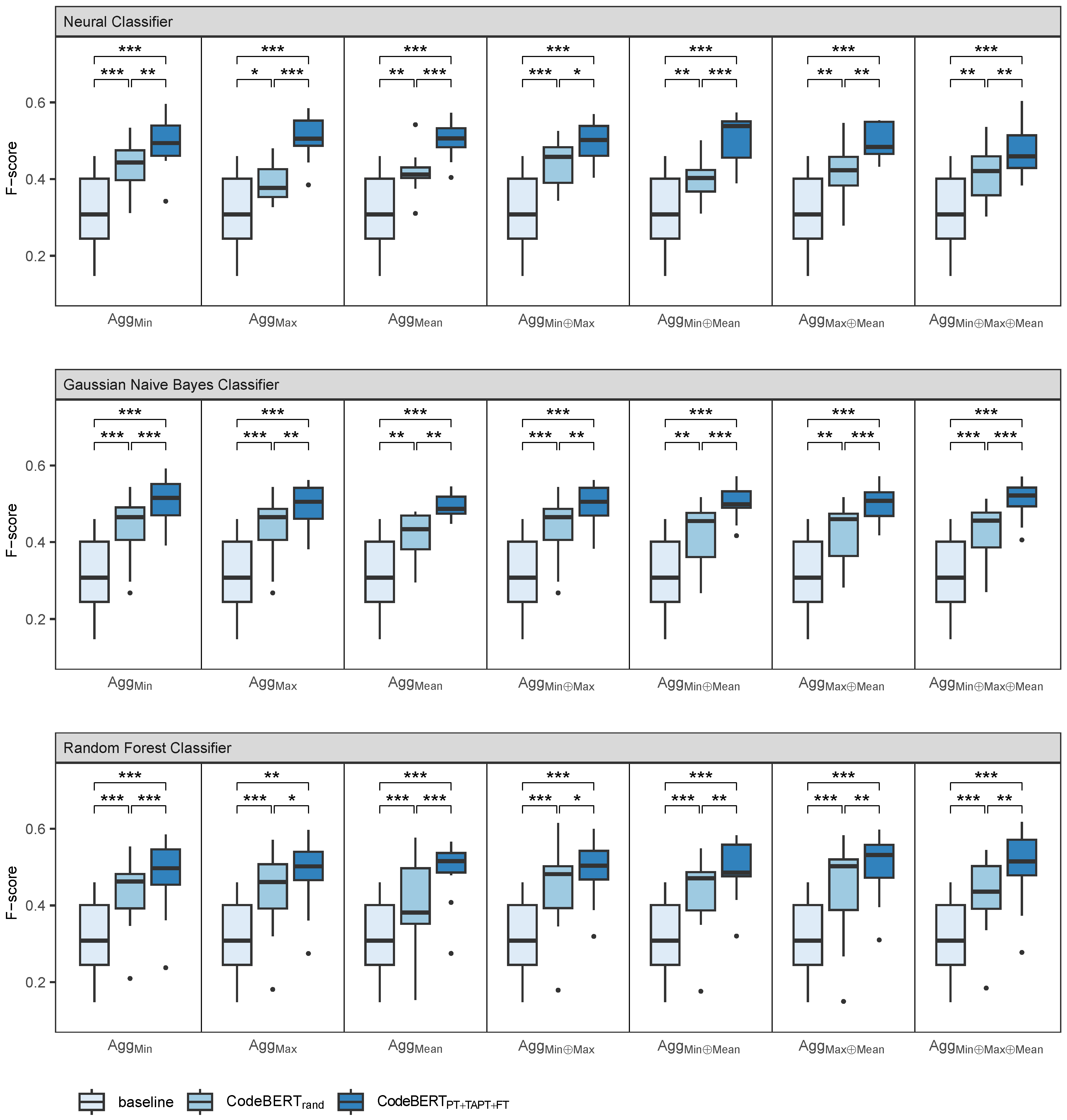
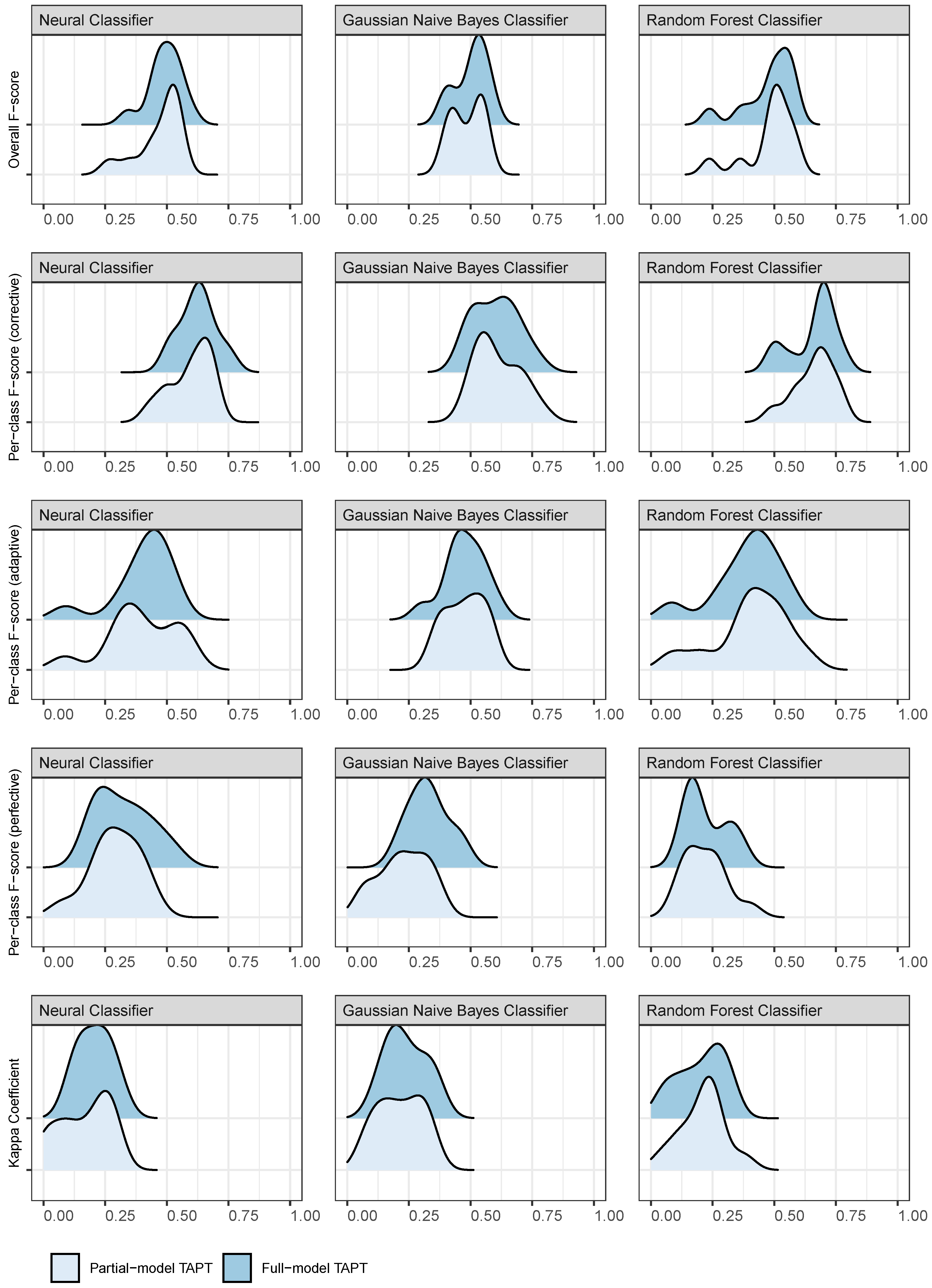
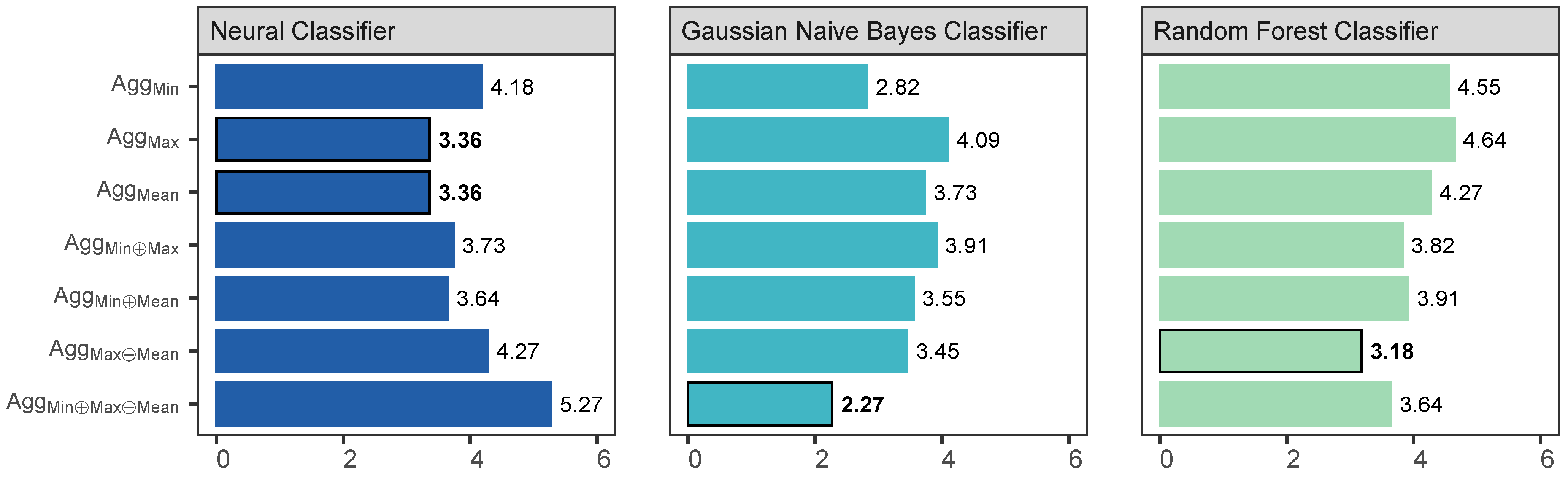
6.1. RQ1 How Effective Is the Proposed Method When Used for Commit Intent Classification?

First, an ablation study was conducted to evaluate the effectiveness of the proposed semantic embedding extraction method and each of its steps for commit intent classification. To explore the impact of the inclusion of the method’s steps on the classification performance, commit intent classification was performed based on the CodeBERT and GraphCodeBERT models with randomly initialized weights (CodeBERT_rand, GraphCodeBERT_rand), general-purpose pre-trained CodeBERT and GraphCodeBERT models (CodeBERT_PT, GraphCodeBERT_PT), fine-tuned pre-trained CodeBERT and GraphCodeBERT models (CodeBERT_PT+FT, GraphCodeBERT_PT+FT), and fine-tuned task-adapted pre-trained CodeBERT and GraphCodeBERT models (CodeBERT_PT+TAPT+FT, GraphCodeBERT_PT+TAPT+FT). In general, the results of the ablation study, reported in

Table 4. Performance of commit intent classification, measured by F-score, using the proposed semantic embedding extraction method with different aggregation techniques and across various classifiers, with an ablation study of the methods’ steps on classification performance.

Neural Classifier
	AggMin	AggMax	AggMean	AggMin⊕Max	AggMin⊕Mean	AggMax⊕Mean	AggMin⊕Max⊕Mean
CodeBERTrand	0.435 ± 0.06	0.392 ± 0.05	0.417 ± 0.06	0.440 ± 0.06	0.403 ± 0.06	0.423 ± 0.07	0.412 ± 0.07
CodeBERTPT	0.475 ± 0.07	0.474 ± 0.07	0.474 ± 0.06	0.467 ± 0.04	0.459 ± 0.08	0.477 ± 0.07	0.474 ± 0.06
CodeBERTPT+FT	0.481 ± 0.09	0.491 ± 0.08	0.492 ± 0.09	0.479 ± 0.08	0.485 ± 0.07	0.481 ± 0.06	0.480 ± 0.08
CodeBERTPT+TAPT+FT	0.493 ± 0.07	0.508 ± 0.06	0.503 ± 0.05	0.498 ± 0.05	0.502 ± 0.07	0.497 ± 0.05	0.472 ± 0.07
GraphCodeBERTrand	0.435 ± 0.06	0.392 ± 0.05	0.417 ± 0.06	0.440 ± 0.06	0.403 ± 0.06	0.423 ± 0.07	0.412 ± 0.07
GraphCodeBERTPT	0.491 ± 0.04	0.468 ± 0.07	0.478 ± 0.05	0.482 ± 0.06	0.481 ± 0.06	0.481 ± 0.04	0.476 ± 0.06
GraphCodeBERTPT+FT	0.482 ± 0.09	0.450 ± 0.10	0.463 ± 0.07	0.452 ± 0.09	0.479 ± 0.07	0.452 ± 0.09	0.484 ± 0.06
GraphCodeBERTPT+TAPT+FT	0.478 ± 0.09	0.461 ± 0.09	0.483 ± 0.08	0.464 ± 0.08	0.466 ± 0.09	0.470 ± 0.08	0.460 ± 0.07
Gaussian Naive Bayes Classifier
	AggMin	AggMax	AggMean	AggMin⊕Max	AggMin⊕Mean	AggMax⊕Mean	AggMin⊕Max⊕Mean
CodeBERTrand	0.437 ± 0.09	0.436 ± 0.09	0.415 ± 0.06	0.436 ± 0.09	0.416 ± 0.08	0.418 ± 0.08	0.422 ± 0.08
CodeBERTPT	0.481 ± 0.07	0.484 ± 0.07	0.439 ± 0.06	0.481 ± 0.07	0.478 ± 0.05	0.475 ± 0.05	0.482 ± 0.06
CodeBERTPT+FT	0.498 ± 0.08	0.491 ± 0.07	0.491 ± 0.08	0.499 ± 0.08	0.485 ± 0.08	0.488 ± 0.07	0.497 ± 0.07
CodeBERTPT+TAPT+FT	0.504 ± 0.07	0.495 ± 0.06	0.495 ± 0.03	0.497 ± 0.06	0.503 ± 0.05	0.500 ± 0.05	0.511 ± 0.05
GraphCodeBERTrand	0.437 ± 0.09	0.436 ± 0.09	0.415 ± 0.06	0.436 ± 0.09	0.416 ± 0.08	0.418 ± 0.08	0.422 ± 0.08
GraphCodeBERTPT	0.439 ± 0.10	0.445 ± 0.09	0.438 ± 0.05	0.442 ± 0.09	0.433 ± 0.08	0.430 ± 0.07	0.432 ± 0.08
GraphCodeBERTPT+FT	0.456 ± 0.08	0.461 ± 0.08	0.483 ± 0.07	0.461 ± 0.08	0.468 ± 0.07	0.464 ± 0.07	0.457 ± 0.07
GraphCodeBERTPT+TAPT+FT	0.456 ± 0.08	0.451 ± 0.08	0.487 ± 0.05	0.454 ± 0.08	0.470 ± 0.05	0.463 ± 0.06	0.461 ± 0.07
Random Forest Classifier
	AggMin	AggMax	AggMean	AggMin⊕Max	AggMin⊕Mean	AggMax⊕Mean	AggMin⊕Max⊕Mean
CodeBERTrand	0.435 ± 0.10	0.436 ± 0.11	0.404 ± 0.12	0.447 ± 0.12	0.433 ± 0.11	0.439 ± 0.13	0.430 ± 0.11
CodeBERTPT	0.485 ± 0.09	0.474 ± 0.10	0.473 ± 0.09	0.482 ± 0.10	0.476 ± 0.09	0.481 ± 0.08	0.490 ± 0.08
CodeBERTPT+FT	0.503 ± 0.10	0.488 ± 0.09	0.495 ± 0.10	0.510 ± 0.10	0.500 ± 0.09	0.502 ± 0.10	0.504 ± 0.09
CodeBERTPT+TAPT+FT	0.481 ± 0.10	0.485 ± 0.09	0.489 ± 0.08	0.495 ± 0.08	0.495 ± 0.08	0.503 ± 0.09	0.499 ± 0.10
GraphCodeBERTrand	0.435 ± 0.10	0.436 ± 0.11	0.404 ± 0.12	0.447 ± 0.12	0.433 ± 0.11	0.439 ± 0.13	0.430 ± 0.11
GraphCodeBERTPT	0.419 ± 0.11	0.448 ± 0.12	0.430 ± 0.10	0.440 ± 0.11	0.444 ± 0.12	0.422 ± 0.11	0.448 ± 0.09
GraphCodeBERTPT+FT	0.465 ± 0.10	0.466 ± 0.12	0.449 ± 0.11	0.465 ± 0.11	0.478 ± 0.10	0.464 ± 0.12	0.464 ± 0.12
GraphCodeBERTPT+TAPT+FT	0.473 ± 0.12	0.453 ± 0.11	0.449 ± 0.11	0.472 ± 0.11	0.482 ± 0.11	0.478 ± 0.10	0.468 ± 0.09

Bold formatting is used to highlight the highest F-score value achieved per a certain aggregation technique for each classifier.

, with the averaged F-score and standard deviation on test datasets across folds, separated by the classifier used and the technique employed for aggregations into commit-level embeddings, show that regardless of the chosen code model, aggregation technique, and classifier, the classification performance gradually improves with each step of the proposed method. When Neural Classifier is used, on average, CodeBERT_PT+TAPT+FT provides an 18.88%, 5.26%, and 2.49% improvement over CodeBERT_rand, CodeBERT_PT, and CodeBERT_PT+FT, respectively, while GraphCodeBERT_PT+TAPT+FT shows a 12.33% improvement over GraphCodeBERT_rand, a 2.24% decrease compared to GraphCodeBERT_PT, and a 0.66% improvement over GraphCodeBERT_PT+FT. With the Gaussian Naive Bayes Classifier, on average, the improvements with CodeBERT_PT+TAPT+FT are 17.69%, 5.56%, and 1.64% over CodeBERT_rand, CodeBERT_PT, and CodeBERT_PT+FT, respectively, while the improvements with GraphCodeBERT_PT+TAPT+FT are 8.87% over GraphCodeBERT_rand, and 5.99% over GraphCodeBERT_PT, while there is a 0.23% decrease compared to GraphCodeBERT_PT+FT. For the Random Forest Classifier with CodeBERT_PT+TAPT+FT, on average, there is a 14.01% improvement over CodeBERT_rand, 2.59% over CodeBERT_PT, yet a 1.59% decrease compared to CodeBERT_PT+FT, while with GraphCodeBERT_PT+TAPT+FT, on average there is a 8.35%, 7.37%, and 0.75% improvement over GraphCodeBERT_rand, GraphCodeBERT_PT, and GraphCodeBERT_PT+FT, respectively. These results demonstrate the effectiveness of the defined steps of the proposed method, i.e., using a pre-trained model, fine-tuning, and task-adaptive pre-training, in improving the commit intent classification performance, alongside the impact that the pre-training on a general corpus and fine-tuning and task-adaptive pre-training on a dataset directly relevant to the classification task have on the overall classification performance. However, it can be observed that the models based on CodeBERT appear to perform better than GraphCodeBERT. This suggests that the semantic features captured by CodeBERT are more effective for commit intent classification than those captured by GraphCodeBERT. Thus, the relationships and dependencies within code that are additionally captured by GraphCodeBERT compared to CodeBERT might not aid in identifying various types of change intent with the herein-proposed semantic embedding extraction method. Given these findings, the subsequent analyses presented in the paper will only focus on CodeBERT-based classification models.

A more comprehensive analysis examined the differences in commit intent classification performances. Figure 3 presents classification performances reported by the F-score of a simple baseline model, i.e., majority class classifier, serving as a reference, and classification models using CodeBERT_rand and CodeBERT_PT+TAPT+FT with different aggregation techniques and classifiers. Annotations in the figure indicate the statistically significant differences among the three comparison groups. Detailed results of the statistical tests are provided in Appendix D in

Table A6. Analysis of the differences in the commit intent classification performances, measured by F-score, between the paired comparisons of the baseline model, and CodeBERT_rand- and CodeBERT_PT+TAPT+FT-based models with various aggregation techniques using Neural Classifier.

Aggregation Technique	Paired Comparison	Shapiro–Wilk Test	Student’s t-Test
AggMin	baseline-CodeBERTrand	W (11) = 0.950, p = 0.648	t (10) = −5.575, p < 0.001 ***
	baseline-CodeBERTPT+TAPT+FT	W (11) = 0.984, p = 0.983	t (10) = −6.845, p < 0.001 ***
	CodeBERTrand-CodeBERTPT+TAPT+FT	W (11) = 0.937, p = 0.486	t (10) = −3.947, p = 0.003 **
AggMax	baseline-CodeBERTrand	W (11) = 0.956, p = 0.719	t (10) = −2.679, p = 0.023 *
	baseline-CodeBERTPT+TAPT+FT	W (11) = 0.901, p = 0.189	t (10) = −6.777, p < 0.001 ***
	CodeBERTrand-CodeBERTPT+TAPT+FT	W (11) = 0.977, p = 0.951	t (10) = −5.784, p < 0.001 ***
AggMean	baseline-CodeBERTrand	W (11) = 0.932, p = 0.429	t (10) = −4.334, p = 0.001 **
	baseline-CodeBERTPT+TAPT+FT	W (11) = 0.939, p = 0.504	t (10) = −8.194, p < 0.001 ***
	CodeBERTrand-CodeBERTPT+TAPT+FT	W (11) = 0.925, p = 0.366	t (10) = −6.456, p < 0.001 ***
AggMin⊕Max	baseline-CodeBERTrand	W (11) = 0.880, p = 0.104	t (10) = −5.331, p < 0.001 ***
	baseline-CodeBERTPT+TAPT+FT	W (11) = 0.858, p = 0.055	t (10) = −7.117, p < 0.001 ***
	CodeBERTrand-CodeBERTPT+TAPT+FT	W (11) = 0.904, p = 0.207	t (10) = −2.856, p = 0.017 *
AggMin⊕Mean	baseline-CodeBERTrand	W (11) = 0.903, p = 0.199	t (10) = −3.394, p = 0.007 **
	baseline-CodeBERTPT+TAPT+FT	W (11) = 0.953, p = 0.686	t (10) = −6.156, p < 0.001 ***
	CodeBERTrand-CodeBERTPT+TAPT+FT	W (11) = 0.961, p = 0.781	t (10) = −4.643, p < 0.001 ***
AggMax⊕Mean	baseline-CodeBERTrand	W (11) = 0.959, p = 0.762	t (10) = −3.739, p = 0.004 **
	baseline-CodeBERTPT+TAPT+FT	W (11) = 0.916, p = 0.287	t (10) = −5.403, p < 0.001 ***
	CodeBERTrand-CodeBERTPT+TAPT+FT	W (11) = 0.932, p = 0.428	t (10) = −4.300, p = 0.002 **
AggMin⊕Max⊕Mean	baseline-CodeBERTrand	W (11) = 0.943, p = 0.556	t (10) = −3.742, p = 0.004 **
	baseline-CodeBERTPT+TAPT+FT	W (11) = 0.942, p = 0.546	t (10) = −7.210, p < 0.001 ***
	CodeBERTrand-CodeBERTPT+TAPT+FT	W (11) = 0.984, p = 0.985	t (10) = −3.903, p = 0.003 **

* p < 0.05, ** p < 0.01, *** p < 0.001.

,

Table A7. Analysis of the differences in the commit intent classification performances, measured by F-score, between the paired comparisons of the baseline model, and CodeBERT_rand- and CodeBERT_PT+TAPT+FT-based models with various aggregation techniques using Gaussian Naive Bayes Classifier.

Aggregation Technique	Paired Comparison	Shapiro–Wilk Test	Student’s t-Test
AggMin	baseline-CodeBERTrand	W (11) = 0.963, p = 0.805	t (10) = −5.790, p < 0.001 ***
	baseline-CodeBERTPT+TAPT+FT	W (11) = 0.921, p = 0.327	t (10) = −6.424, p < 0.001 ***
	CodeBERTrand-CodeBERTPT+TAPT+FT	W (11) = 0.924, p = 0.353	t (10) = −4.853, p < 0.001 ***
AggMax	baseline-CodeBERTrand	W (11) = 0.962, p = 0.801	t (10) = −5.794, p < 0.001 ***
	baseline-CodeBERTPT+TAPT+FT	W (11) = 0.923, p = 0.343	t (10) = −6.316, p < 0.001 ***
	CodeBERTrand-CodeBERTPT+TAPT+FT	W (11) = 0.943, p = 0.555	t (10) = −4.126, p = 0.002 **
AggMean	baseline-CodeBERTrand	W (11) = 0.929, p = 0.400	t (10) = −3.297, p = 0.008 **
	baseline-CodeBERTPT+TAPT+FT	W (11) = 0.882, p = 0.111	t (10) = −5.451, p < 0.001 ***
	CodeBERTrand-CodeBERTPT+TAPT+FT	W (11) = 0.934, p = 0.456	t (10) = −4.456, p = 0.001 **
AggMin⊕Max	baseline-CodeBERTrand	W (11) = 0.966, p = 0.845	t (10) = −5.874, p < 0.001 ***
	baseline-CodeBERTPT+TAPT+FT	W (11) = 0.926, p = 0.375	t (10) = −6.444, p < 0.001 ***
	CodeBERTrand-CodeBERTPT+TAPT+FT	W (11) = 0.949, p = 0.635	t (10) = −4.272, p = 0.002 **
AggMin⊕Mean	baseline-CodeBERTrand	W (11) = 0.955, p = 0.707	t (10) = −3.746, p = 0.004 **
	baseline-CodeBERTPT+TAPT+FT	W (11) = 0.907, p = 0.223	t (10) = −6.305, p < 0.001 ***
	CodeBERTrand-CodeBERTPT+TAPT+FT	W (11) = 0.877, p = 0.094	t (10) = −5.829, p < 0.001 ***
AggMax⊕Mean	baseline-CodeBERTrand	W (11) = 0.955, p = 0.707	t (10) = −3.928, p = 0.003 **
	baseline-CodeBERTPT+TAPT+FT	W (11) = 0.880, p = 0.104	t (10) = −6.152, p < 0.001 ***
	CodeBERTrand-CodeBERTPT+TAPT+FT	W (11) = 0.957, p = 0.736	t (10) = −5.628, p < 0.001 ***
AggMin⊕Max⊕Mean	baseline-CodeBERTrand	W (11) = 0.967, p = 0.855	t (10) = −4.871, p < 0.001 ***
	baseline-CodeBERTPT+TAPT+FT	W (11) = 0.886, p = 0.123	t (10) = −7.150, p < 0.001 ***
	CodeBERTrand-CodeBERTPT+TAPT+FT	W (11) = 0.953, p = 0.683	t (10) = −7.096, p < 0.001 ***

** p < 0.01, *** p < 0.001.

and

Table A8. Analysis of the differences in the commit intent classification performances, measured by F-score, between the paired comparisons of the baseline model, and CodeBERT_rand- and CodeBERT_PT+TAPT+FT-based models with various aggregation techniques using Random Forest Classifier.

Aggregation Technique	Paired Comparison	Shapiro–Wilk Test	Student’s t-Test/Wilcoxon Signed-Rank Test
AggMin	baseline-CodeBERTrand	W (11) = 0.945, p = 0.579	t (10) = −7.296, p < 0.001 ***
	baseline-CodeBERTPT+TAPT+FT	W (11) = 0.885, p = 0.121	t (10) = −9.483, p < 0.001 ***
	CodeBERTrand-CodeBERTPT+TAPT+FT	W (11) = 0.951, p = 0.663	t (10) = −5.389, p < 0.001 ***
AggMax	baseline-CodeBERTrand	W (11) = 0.953, p = 0.678	t (10) = −5.203, p < 0.001 ***
	baseline-CodeBERTPT+TAPT+FT	W (11) = 0.849, p = 0.042 *	Z = 2.934, p = 0.003 **
	CodeBERTrand-CodeBERTPT+TAPT+FT	W (11) = 0.957, p = 0.728	t (10) = −2.517, p = 0.031 *
AggMean	baseline-CodeBERTrand	W (11) = 0.947, p = 0.610	t (10) = −7.342, p < 0.001 ***
	baseline-CodeBERTPT+TAPT+FT	W (11) = 0.890, p = 0.138	t (10) = −8.770, p < 0.001 ***
	CodeBERTrand-CodeBERTPT+TAPT+FT	W (11) = 0.920, p = 0.315	t (10) = −4.733, p < 0.001 ***
AggMin⊕Max	baseline-CodeBERTrand	W (11) = 0.961, p = 0.783	t (10) = −6.407, p < 0.001 ***
	baseline-CodeBERTPT+TAPT+FT	W (11) = 0.948, p = 0.614	t (10) = −10.243, p < 0.001 ***
	CodeBERTrand-CodeBERTPT+TAPT+FT	W (11) = 0.930, p = 0.407	t (10) = −2.451, p = 0.034 *
AggMin⊕Mean	baseline-CodeBERTrand	W (11) = 0.981, p = 0.973	t (10) = −6.896, p < 0.001 ***
	baseline-CodeBERTPT+TAPT+FT	W (11) = 0.934, p = 0.453	t (10) = −8.912, p < 0.001 ***
	CodeBERTrand-CodeBERTPT+TAPT+FT	W (11) = 0.894, p = 0.157	t (10) = −3.993, p = 0.003 **
AggMax⊕Mean	baseline-CodeBERTrand	W (11) = 0.963, p = 0.813	t (10) = −5.107, p < 0.001 ***
	baseline-CodeBERTPT+TAPT+FT	W (11) = 0.934, p = 0.457	t (10) = −10.523, p < 0.001 ***
	CodeBERTrand-CodeBERTPT+TAPT+FT	W (11) = 0.955, p = 0.709	t (10) = −3.371, p = 0.007 **
AggMin⊕Max⊕Mean	baseline-CodeBERTrand	W (11) = 0.889, p = 0.135	t (10) = −6.231, p < 0.001 ***
	baseline-CodeBERTPT+TAPT+FT	W (11) = 0.920, p = 0.321	t (10) = −7.609, p < 0.001 ***
	CodeBERTrand-CodeBERTPT+TAPT+FT	W (11) = 0.783, p = 0.006 **	Z = 2.934, p = 0.003 **

* p < 0.05, ** p < 0.01, *** p < 0.001.

for the Neural, Gaussian Naive Bayes, and Random Forest Classifiers, respectively. Depending on the data distribution, appropriate tests were applied. Where the Shapiro–Wilk test showed that the distribution of the differences in F-score was not significantly different from a normal distribution (e.g., W(11) = 0.950, p = 0.648 in the case of baseline-CodeBERT_PT+TAPT+FT using Agg_Min and the Neural Classifier), the Student’s paired-samples t-test was used to assess the differences in classification performance. Alternatively, where the Shapiro–Wilk test showed that the differences in F-score did not meet the assumption of normality (e.g., W(11) = 0.849, p = 0.042 for baseline-CodeBERT_PT+TAPT+FT using Agg_Max and the Random Forest Classifier), the Wilcoxon signed-rank test was used. The analysis confirms statistically significant performance differences across all classifiers and aggregation techniques between the three classification models, i.e., between the baseline and CodeBERT_rand, baseline and CodeBERT_PT+TAPT+FT, as well as between CodeBERT_rand and CodeBERT_PT+TAPT+FT. In each paired comparison, the classification performance of the latter model is statistically significantly better. These findings reveal that even when utilizing a code model with randomly initialized weights, the resulting classification models can distinguish between various types of intents to a limited extent, outperforming the majority class baseline. Thus, the increased complexity of the model, resulting from the incorporation of a code model, in comparison to the baseline reference, indeed leads to enhanced performance. At the same time, these findings indicate that the inherent architecture of the code model, even without pre-training, is capable of capturing certain patterns in the data relevant to change intent; a phenomenon of language models with random parameterizations that prior studies have already discussed [65,81,82]. Nevertheless, a significant difference in performance can be observed when a code model with a fine-tuned task-adaptive pre-training strategy is employed, marking significant improvements over its randomly initialized counterpart.

To further analyze the ability of the three models to distinguish between the three classes of commit intents, Figure 4 presents the normalized confusion matrices for the test dataset across all folds. These matrices compare the performance of a majority class baseline model with classification models based on CodeBERT_rand and CodeBERT_PT+TAPT+FT on the example of using the Agg_Max aggregation technique and Neural Classifier. The baseline model classifies all commits as corrective. As it does not correctly identify any commits of the other two classes, this shows its inability to distinguish between change intents. In comparison, the CodeBERT_rand-based classification model achieves a more balanced classification across the three classes, though with a persistent bias towards the corrective class. The model is able to classify 54.1% of corrective, 32.4% of adaptive, and 17.9% of perfective commits correctly, yet incorrectly classifies 47.1% and 52% of adaptive and perfective commits, respectively, as corrective. In contrast, the CodeBERT_PT+TAPT+FT-based classification model demonstrates a better per-class classification performance than the previously discussed models. The model can correctly classify 64.7% of corrective, 41% of adaptive, and 37.1% of perfective commits, indicating it performs better for all three classes. There is still considerable confusion between classes, but it is reduced compared to the CodeBERT_rand-based model. Overall, although the improvement in classification performance from the baseline through CodeBERT_rand to CodeBERT_PT+TAPT+FT can be observed, and the models become progressively better at distinguishing between different types of intents, there are still considerable misclassifications present, suggesting that the proposed method has potential for further improvement to achieve even better classification performance.

As task-adaptive pre-training can be computationally heavy, studies have shown that training only a part of the language model, where not all parameters are trainable during task adaptation, can still provide comparative results compared to training the entire model. To assess this in the context of commit intent classification, we analyzed the influence of the two training strategies of task-adaptive pre-training, i.e., full-model and partial-model training, on commit intent classification performance. This was achieved by observing the differences in performance, measured by the overall F-score, per-class F-score (for corrective, adaptive, and perfective classes), and Kappa Coefficient under the same experimental settings aside from the training strategy. In our experimental design, the partial-model training involved training only 31.8% of the model’s parameters during task adaptation. Similar to before, depending on the data distribution, appropriate tests were applied: either the Student’s paired-samples t-test, which was used when the assumptions of normality, assessed by the Shapiro–Wilk test, were met or the non-parametric counterpart, the Wilcoxon signed-rank test, when the assumptions of normality were not met. Detailed results of the statistical tests are provided in Appendix D in

Table A9. Analysis of the differences in the commit intent classification performances, measured by F-score, per-class F-scores, and Kappa Coefficient, between the paired comparisons of the CodeBERT_PT+TAPT+FT-based models using partial-model and full-model task-adaptive pre-training with various aggregation techniques using Neural Classifier.

Aggregation Technique	Performance Metric	Shapiro–Wilk Test	Student’s t-Test
AggMin	F-score	W (11) = 0.959, p = 0.762	t (10) = −1.455, p = 0.176
	Per-class F-score (corrective)	W (11) = 0.963, p = 0.807	t (10) = −1.728, p = 0.115
	Per-class F-score (adaptive)	W (11) = 0.970, p = 0.888	t (10) = −0.393, p = 0.702
	Per-class F-score (perfective)	W (11) = 0.895, p = 0.162	t (10) = −1.062, p = 0.313
	Kappa Coefficient	W (11) = 0.948, p = 0.621	t (10) = −1.883, p = 0.089
AggMean	F-score	W (11) = 0.956, p = 0.717	t (10) = −1.664, p = 0.127
	Per-class F-score (corrective)	W (11) = 0.877, p = 0.096	t (10) = −1.585, p = 0.144
	Per-class F-score (adaptive)	W (11) = 0.920, p = 0.316	t (10) = −0.212, p = 0.836
	Per-class F-score (perfective)	W (11) = 0.921, p = 0.328	t (10) = −1.164, p = 0.272
	Kappa Coefficient	W (11) = 0.947, p = 0.606	t (10) = −1.551, p = 0.152
AggMax	F-score	W (11) = 0.867, p = 0.070	t (10) = −1.463, p = 0.174
	Per-class F-score (corrective)	W (11) = 0.909, p = 0.239	t (10) = −0.452, p = 0.661
	Per-class F-score (adaptive)	W (11) = 0.960, p = 0.775	t (10) = −0.712, p = 0.493
	Per-class F-score (perfective)	W (11) = 0.943, p = 0.560	t (10) = −1.698, p = 0.120
	Kappa Coefficient	W (11) = 0.920, p = 0.318	t (10) = −1.543, p = 0.154
AggMin⊕Max	F-score	W (11) = 0.938, p = 0.494	t (10) = −0.759, p = 0.465
	Per-class F-score (corrective)	W (11) = 0.988, p = 0.994	t (10) = −0.317, p = 0.758
	Per-class F-score (adaptive)	W (11) = 0.890, p = 0.139	t (10) = −0.379, p = 0.713
	Per-class F-score (perfective)	W (11) = 0.944, p = 0.566	t (10) = −1.406, p = 0.190
	Kappa Coefficient	W (11) = 0.904, p = 0.206	t (10) = −0.927, p = 0.376
AggMin⊕Mean	F-score	W (11) = 0.936, p = 0.473	t (10) = −1.574, p = 0.147
	Per-class F-score (corrective)	W (11) = 0.913, p = 0.264	t (10) = −0.385, p = 0.708
	Per-class F-score (adaptive)	W (11) = 0.941, p = 0.527	t (10) = −2.401, p = 0.037 *
	Per-class F-score (perfective)	W (11) = 0.984, p = 0.983	t (10) = −1.663, p = 0.127
	Kappa Coefficient	W (11) = 0.872, p = 0.082	t (10) = −1.670, p = 0.126
AggMax⊕Mean	F-score	W (11) = 0.918, p = 0.300	t (10) = −0.561, p = 0.587
	Per-class F-score (corrective)	W (11) = 0.931, p = 0.422	t (10) = 0.322, p = 0.754
	Per-class F-score (adaptive)	W (11) = 0.954, p = 0.690	t (10) = −0.056, p = 0.956
	Per-class F-score (perfective)	W (11) = 0.931, p = 0.423	t (10) = −1.327, p = 0.214
	Kappa Coefficient	W (11) = 0.892, p = 0.146	t (10) = −0.587, p = 0.570
AggMin⊕Max⊕Mean	F-score	W (11) = 0.947, p = 0.608	t (10) = 0.813, p = 0.435
	Per-class F-score (corrective)	W (11) = 0.875, p = 0.091	t (10) = 0.203, p = 0.843
	Per-class F-score (adaptive)	W (11) = 0.913, p = 0.263	t (10) = 0.512, p = 0.620
	Per-class F-score (perfective)	W (11) = 0.937, p = 0.488	t (10) = −0.311, p = 0.762
	Kappa Coefficient	W (11) = 0.973, p = 0.913	t (10) = −0.209, p = 0.839

* p < 0.05.

,

Table A10. Analysis of the differences in the commit intent classification performances, measured by F-score, per-class F-scores, and Kappa Coefficient, between the paired comparisons of the CodeBERT_PT+TAPT+FT-based models using partial-model and full-model task-adaptive pre-training with various aggregation techniques using Gaussian Naive Bayes Classifier.

Aggregation Technique	Performance Metric	Shapiro–Wilk Test	Student’s t-Test/Wilcoxon Signed-Rank Test
AggMin	F-score	W (11) = 0.811, p = 0.013 *	Z = 1.334, p = 0.182
	Per-class F-score (corrective)	W (11) = 0.900, p = 0.187	t (10) = 0.848, p = 0.416
	Per-class F-score (adaptive)	W (11) = 0.945, p = 0.578	t (10) = −0.011, p = 0.992
	Per-class F-score (perfective)	W (11) = 0.968 p = 0.865	t (10) = −3.321, p = 0.008 **
	Kappa Coefficient	W (11) = 0.877, p = 0.095	t (10) = −1.920, p = 0.084
AggMean	F-score	W (11) = 0.869, p = 0.076	t (10) = −0.154, p = 0.881
	Per-class F-score (corrective)	W (11) = 0.937, p = 0.491	t (10) = −0.174, p = 0.865
	Per-class F-score (adaptive)	W (11) = 0.910, p = 0.241	t (10) = 0.804, p = 0.440
	Per-class F-score (perfective)	W (11) = 0.969, p = 0.874	t (10) = −1.231, p = 0.246
	Kappa Coefficient	W (11) = 0.940, p = 0.519	t (10) = −0.223, p = 0.828
AggMax	F-score	W (11) = 0.951, p = 0.658	t (10) = −1.585, p = 0.144
	Per-class F-score (corrective)	W (11) = 0.850, p = 0.043 *	Z = 0.356, p = 0.722
	Per-class F-score (adaptive)	W (11) = 0.979, p = 0.960	t (10) = 0.744, p = 0.474
	Per-class F-score (perfective)	W (11) = 0.951, p = 0.657	t (10) = −2.829, p = 0.018 *
	Kappa Coefficient	W (11) = 0.982, p = 0.978	t (10) = −2.127, p = 0.059
AggMin⊕Max	F-score	W (11) = 0.980, p = 0.966	t (10) = −2.394, p = 0.038 *
	Per-class F-score (corrective)	W (11) = 0.918, p = 0.302	t (10) = 0.166, p = 0.872
	Per-class F-score (adaptive)	W (11) = 0.980, p = 0.964	t (10) = 0.489, p = 0.635
	Per-class F-score (perfective)	W (11) = 0.951, p = 0.653	t (10) = −3.638, p = 0.005 **
	Kappa Coefficient	W (11) = 0.926, p = 0.371	t (10) = −3.285, p = 0.008 **
AggMin⊕Mean	F-score	W (11) = 0.883, p = 0.115	t (10) = −1.209, p = 0.255
	Per-class F-score (corrective)	W (11) = 0.935, p = 0.467	t (10) = −0.596, p = 0.565
	Per-class F-score (adaptive)	W (11) = 0.971, p = 0.895	t (10) = 1.168, p = 0.270
	Per-class F-score (perfective)	W (11) = 0.970, p = 0.890	t (10) = −3.314, p = 0.008 **
	Kappa Coefficient	W (11) = 0.946, p = 0.592	t (10) = −1.480, p = 0.170
AggMax⊕Mean	F-score	W (11) = 0.883, p = 0.113	t (10) = −0.859, p = 0.411
	Per-class F-score (corrective)	W (11) = 0.980, p = 0.968	t (10) = −0.419, p = 0.684
	Per-class F-score (adaptive)	W (11) = 0.914, p = 0.269	t (10) = 0.762, p = 0.463
	Per-class F-score (perfective)	W (11) = 0.902, p = 0.194	t (10) = −2.654, p = 0.024 *
	Kappa Coefficient	W (11) = 0.960, p = 0.771	t (10) = −1.041, p = 0.323
AggMin⊕Max⊕Mean	F-score	W (11) = 0.921, p = 0.330	t (10) = −2.132, p = 0.059
	Per-class F-score (corrective)	W (11) = 0.893, p = 0.151	t (10) = −1.007, p = 0.338
	Per-class F-score (adaptive)	W (11) = 0.766, p = 0.003 **	Z = −0.178, p = 0.859
	Per-class F-score (perfective)	W (11) = 0.956, p = 0.721	t (10) = −3.349, p = 0.007 **
	Kappa Coefficient	W (11) = 0.960, p = 0.773	t (10) = −2.447, p = 0.034 *

* p < 0.05, ** p < 0.01.

and

Table A11. Analysis of the differences in the commit intent classification performances, measured by F-score, per-class F-scores, and Kappa Coefficient, between the paired comparisons of the CodeBERT_PT+TAPT+FT-based models using partial-model and full-model task-adaptive pre-training with various aggregation techniques using Random Forest Classifier.

Aggregation Technique	Performance Metric	Shapiro–Wilk Test	Student’s t-Test/Wilcoxon Signed-Rank Test
AggMin	F-score	W (11) = 0.859, p = 0.056	t (10) = 0.276, p = 0.788
	Per-class F-score (corrective)	W (11) = 0.960, p = 0.777	t (10) = 0.107, p = 0.917
	Per-class F-score (adaptive)	W (11) = 0.893, p = 0.149	t (10) = 0.422, p = 0.682
	Per-class F-score (perfective)	W (11) = 0.888, p = 0.131	t (10) = −0.305, p = 0.767
	Kappa Coefficient	W (11) = 0.911, p = 0.252	t (10) = 0.423, p = 0.682
AggMean	F-score	W (11) = 0.953, p = 0.686	t (10) = −225, p = 0.826
	Per-class F-score (corrective)	W (11) = 0.919, p = 0.308	t (10) = 0.123, p = 0.904
	Per-class F-score (adaptive)	W (11) = 0.942, p = 0.547	t (10) = 0.479, p = 0.642
	Per-class F-score (perfective)	W (11) = 0.952, p = 0.670	t (10) = −0.906, p = 0.386
	Kappa Coefficient	W (11) = 0.912, p = 0.260	t (10) = −0.334, p = 0.745
AggMax	F-score	W (11) = 0.949, p = 0.628	t (10) = 0.699, p = 0.500
	Per-class F-score (corrective)	W (11) = 0.956, p = 0.727	t (10) = 0.258, p = 0.801
	Per-class F-score (adaptive)	W (11) = 0.961, p = 0.786	t (10) = 0.146, p = 0.887
	Per-class F-score (perfective)	W (11) = 0.967, p = 0.850	t (10) = 0.396, p = 0.700
	Kappa Coefficient	W (11) = 0.954, p = 0.701	t (10) = 0.546, p = 0.597
AggMin⊕Max	F-score	W (11) = 0.948, p = 0.614	t (10) = 0.559, p = 0.589
	Per-class F-score (corrective)	W (11) = 0.811, p = 0.013 *	Z = −0.764, p = 0.445
	Per-class F-score (adaptive)	W (11) = 0.899, p = 0.182	t (10) = 1.115, p = 0.291
	Per-class F-score (perfective)	W (11) = 0.958, p = 0.745	t (10) = 0.073, p = 0.943
	Kappa Coefficient	W (11) = 0.914, p = 0.274	t (10) = 0.548, p = 0.596
AggMin⊕Mean	F-score	W (11) = 0.851, p = 0.044 *	Z = 0.000, I = 1.000
	Per-class F-score (corrective)	W (11) = 0.888, p = 0.133	t (10) = −0.115, p = 0.910
	Per-class F-score (adaptive)	W (11) = 0.777, p = 0.005 **	Z = 0.764, p = 0.445
	Per-class F-score (perfective)	W (11) = 0.971, p = 0.896	t (10) = −0.085, p = 0.934
	Kappa Coefficient	W (11) = 0.928, p = 0.388	t (10) = −0.551, p = 0.593
AggMax⊕Mean	F-score	W (11) = 0.961, p = 0.785	t (10) = −0.965, p = 0.357
	Per-class F-score (corrective)	W (11) = 0.892, p = 0.146	t (10) = −0.277, p = 0.787
	Per-class F-score (adaptive)	W (11) = 0.945, p = 0.584	t (10) = −0.343, p = 0.739
	Per-class F-score (perfective)	W (11) = 0.960, p = 0.778	t (10) = −1.370, p = 0.201
	Kappa Coefficient	W (11) = 0.935, p = 0.469	t (10) = −0.835, p = 0.423
AggMin⊕Max⊕Mean	F-score	W (11) = 0.983, p = 0.980	t (10) = −0.090, p = 0.930
	Per-class F-score (corrective)	W (11) = 0.812, p = 0.013 *	Z = −0.968, p = 0.333
	Per-class F-score (adaptive)	W (11) = 0.940, p = 0.517	t (10) = −0.205, p = 0.841
	Per-class F-score (perfective)	W (11) = 0.800, p = 0.010 *	Z = 1.260, p = 0.208
	Kappa Coefficient	W (11) = 0.939, p = 0.505	t (10) = 0.048, p = 0.962

* p < 0.05, ** p < 0.01.

for the Neural, Gaussian Naive Bayes, and Random Forest Classifiers, respectively. To illustrate the differences in classification performance between the two training approaches, Figure 5 represents the distribution of performance on the commit intent classification models based on CodeBERT_PT+TAPT+FT with Agg_Min aggregation technique, using full-model and partial-model task adaptation. In a large majority of observations, the results show that there are no statistically significant differences in classification performance between the two training strategies. More specifically, in 95.2%, 100%, 95.2%, 71.4%, and 90.5% of observations, no statistically significant differences were observed in terms of F-score, per-class F-score for the corrective class, per-class F-score for the adaptive class, per-class F-score for the perfective class, and Kappa Coefficient, respectively. Only in one observation was the F-score statistically significantly higher for full-model training than partial-model training (in the case of Agg_Min⊕Max using the Gaussian Naive Bayes Classifier). In two cases, the Kappa Coefficient was statistically significantly higher for full-model training than partial-model training (in the cases of Agg_Min⊕Max and Agg_{Min⊕Max⊕Mean} using the Gaussian Naive Bayes Classifier). In one case, the per-class F-score for the adaptive class was statistically significantly higher for full-model training compared to partial-model training. In six cases, the per-class F-score for the perfective class was statistically significantly higher for full-model training compared to partial-model training. These findings suggest that task-adaptive pre-training can be conducted effectively with only partial-model training to reduce the computational resources needed without significantly sacrificing classification performance. This is especially relevant for environments with limited computational resources. This might be due to the similarity between the pre-training and target tasks, where the representations learned during pre-training are already well-suited to the target task. Consequently, adapting the model by partially adjusting the weights is almost as effective as adapting all weights.

Lastly, as part of the proposed method, we evaluated the different aggregation techniques used within the experiments. Separated by the classifier used, each aggregation technique was assigned a rank from one to seven based on its classification performance per fold on CodeBERT_PT+TAPT+FT, with rank one representing the highest and seven the lowest performance in terms of the F-score in a fold. To gain deeper insight into the effectiveness of the aggregation techniques, we averaged the per-fold ranks across all folds. The resulting averaged ranks, presented in Figure 6, provide a rough estimate of each aggregation technique’s overall performance, where a lower rank signifies better average performance across folds for a specific classifier. Although previous analyses have already shown varying performances across different aggregation techniques, the ranks presented here demonstrate that no single technique consistently outperforms the others across all three classifiers. For the Neural Classifier, the best-performing techniques are Agg_Max and Agg_Mean. The top technique for the Gaussian Naive Bayes Classifier is Agg_{Min⊕Max⊕Mean}. For Random Forest Classifier, Agg_Max⊕Mean performs the best. It appears that the techniques performing the best with the Neural Classifier are the least effective for the Gaussian Naive Bayes Classifier, and vice versa. These observations suggest that while certain combinations of classifiers and aggregation techniques may yield optimal results for commit intent classification, further exploring these combinations is beyond the scope of this paper. Furthermore, our findings underscore the potential need for developing task-specific aggregation techniques that could more effectively address the target task, for instance, by considering relationships between changes, as opposed to the simple dimension-wise aggregation approaches employed in this study.

6.2. RQ2 How Does the Proposed Method Compare to the SOTA When Used for Commit Intent Classification?

To benchmark the classification performance of models using the proposed semantic commit feature extraction method against the current SOTA, we employed the best-performing aggregation technique for each classifier, identified by the analysis in the context of RQ1, to build commit intent classification models based on the proposed method. Specifically, for the Neural Classifier, we used CodeBERT_PT+TAPT+FT with Agg_Max. For Gaussian Naive Bayes, we combined CodeBERT_PT+TAPT+FT with Agg_{Min⊕Max⊕Mean}, and for Random Forest, we used CodeBERT_PT+TAPT+FT with Agg_Max⊕Mean. In

Table 5. Comparative analysis of the classification performance, measured by F-score and Kappa Coefficient, of commit intent classification models based on the proposed method in comparison to the SOTA.

Neural Classifier
Paired Comparison	Performance Metric	Avg1	Avg2	Shapiro–Wilk Test	Student’s t-Test
proposed method–Levin and Yehudai [22]	F-score	0.509	0.516	W(11) = 0.957, p = 0.735	t(10) = −0.287, p = 0.780
	Kappa Coefficient	0.232	0.221	W(11) = 0.963, p = 0.804	t(10) = 0.317, p = 0.758
proposed method–Hönel et al. [7]	F-score	0.509	0.525	W(11) = 0.938, p = 0.492	t(10) = −0.870, p = 0.405
	Kappa Coefficient	0.232	0.248	W(11) = 0.920, p = 0.320	t(10) = −0.542, p = 0.599
proposed method–Ghadhab et al. [14]	F-score	0.509	0.414	W(11) = 0.914, p = 0.274	t(10) = 3.728, p = 0.004 **
	Kappa Coefficient	0.232	0.109	W(11) = 0.980, p = 0.964	t(10) = 3.738, p = 0.004 **
proposed method–Mariano et al. [15]	F-score	0.509	0.529	W(11) = 0.882, p = 0.110	t(10) = −1.285, p = 0.228
	Kappa Coefficient	0.232	0.250	W(11) = 0.911, p = 0.251	t(10) = −0.637, p = 0.539
Gaussian Naive Bayes Classifier
Paired Comparison	Performance Metric	Avg1	Avg2	Shapiro–Wilk Test	Student’s t-Test/Wilcoxon Signed-Rank Test
proposed method–Levin and Yehudai [22]	F-score	0.511	0.450	W(11) = 0.911, p = 0.249	t(10) = 1.600, p = 0.141
	Kappa Coefficient	0.248	0.166	W(11) = 0.955, p = 0.708	t(10) = 2.016, p = 0.072
proposed method–Hönel et al. [7]	F-score	0.511	0.429	W(11) = 0.940, p = 0.521	t(10) = 3.524, p = 0.006 **
	Kappa Coefficient	0.248	0.126	W(11) = 0.929, p = 0.400	t(10) = 6.305, p < 0.001 ***
proposed method–Ghadhab et al. [14]	F-score	0.511	0.373	W(11) = 0.969, p = 0.872	t(10) = 6.034, p < 0.001 ***
	Kappa Coefficient	0.248	0.058	W(11) = 0.958, p = 0.752	t(10) = 9.758, p < 0.001 ***
proposed method–Mariano et al. [15]	F-score	0.511	0.406	W(11) = 0.917, p = 0.295	t(10) = 3.518, p = 0.006 **
	Kappa Coefficient	0.248	0.100	W(11) = 0.701, p < 0.001 ***	Z = −2.845, p = 0.004 **
Random Forest Classifier
Paired Comparison	Performance Metric	Avg1	Avg2	Shapiro–Wilk Test	Student’s t-Test
proposed method–Levin and Yehudai [22]	F-score	0.501	0.467	W(11) = 0.894, p = 0.157	t(10) = 2.768, p = 0.020 *
	Kappa Coefficient	0.220	0.164	W(11) = 0.878, p = 0.097	t(10) = 2.425, p = 0.036 *
proposed method–Hönel et al. [7]	F-score	0.501	0.503	W(11) = 0.976, p = 0.939	t(10) = −0.101, p = 0.922
	Kappa Coefficient	0.220	0.217	W(11) = 0.969, p = 0.879	t(10) = 0.100, p = 0.922
proposed method–Ghadhab et al. [14]	F-score	0.501	0.402	W(11) = 0.932, p = 0.429	t(10) = 3.945, p = 0.003 **
	Kappa Coefficient	0.220	0.102	W(11) = 0.947, p = 0.603	t(10) = 3.289, p = 0.008 **
proposed method–Mariano et al. [15]	F-score	0.501	0.533	W(11) = 0.951, p = 0.656	t(10) = −1.633, p = 0.133
	Kappa Coefficient	0.220	0.256	W(11) = 0.968, p = 0.869	t(10) = −1.461, p = 0.175

Avg = average, * p < 0.05, ** p < 0.01, *** p < 0.001.

, we present the average classification performance, measured by F-score and Kappa Coefficient, of the commit intent classification models based on the proposed method with the aforementioned settings and on SOTA, alongside comparative analysis of the differences in classification performance for each paired comparison. Appropriate statistical tests were applied based on the data distribution to evaluate performance differences. Again, based upon the results of the Shapiro–Wilk test, either the Student’s paired-samples t-test or the Wilcoxon signed-rank test was used. Across all comparisons, our proposed method’s classification model demonstrated performance comparable to, and in several instances superior to, the SOTA models. Specifically, in the majority of comparisons, the proposed method’s classification performance outperformed that of the SOTA. Notably, in 50.0% of these comparisons, the difference in performance in favor of the proposed method was statistically significant. At the same time, there were no observed comparisons where the SOTA-based classification models statistically outperformed those based on the proposed method. For instance, with the Gaussian Naive Bayes Classifier, the models based on the proposed method outperform all SOTA-based models, with a statistically significant difference in performance compared to classification models based on features proposed by Hönel et al. [7], Ghadhab et al. [14], and Mariano et al. [15]. In the case of the model based on features proposed by Levin and Yehudai [22], although the model based on the proposed method yielded a higher average F-score and Kappa Coefficient, the performance differences were not statistically significant. These results demonstrate the effectiveness of the proposed method despite it representing the first attempt to apply semantic source code embeddings for commit intent classification. While further research is necessary to build upon these initial findings, the work presented in this paper lays a strong foundation, indicating performance that is not only comparable but, in many cases, superior to the existing SOTA.

7. Threats to Validity

7.1. Threats to Construct Validity

To address the threat to construct validity related to inadequately defined concepts, we provide precise definitions of software change intents by referring to an existing, widely accepted, and the most frequently used intent-based categorization scheme of software maintenance activities, introduced by Swanson [20]. It is important to note that the selected categorization scheme and presented definitions are in alignment with the ones used to prepare a labeled dataset on which our work is built. Our work has a construct representation bias regarding how software changes are represented. When embedding commits with a fine-tuned task-adapted pre-trained transformer-based code model, only modified code lines are taken into account. This might neglect the surrounding context in which the changes are made, e.g., the project’s domain, the part of the modified codebase (i.e., production or test), and the code context in which the code lines are modified. To address the threat of construct under-representation related to mono-operation bias, we operationalize classification model performance by employing several measures, including F-score, and Cohen’s Kappa Coefficient. By using multiple metrics, we mitigate a narrow interpretation of models’ performances and obtain a more comprehensive evaluation as different metrics capture different aspects of classification performance. However, we do not consider any other metrics that could address the performance in terms of the training and use of the model, e.g., model complexity, time complexity of training, and inference time, which may present intriguing research directions for future studies.

7.2. Threats to Internal Validity

There is a threat to internal validity related to anomalies in instrumentation, i.e., tools and procedures. To ensure reliability and consistency in the data preparation procedure, data are gathered using GitHub REST API, GitPython, and codeprep along with our custom implementations when needed. Existing tools are used preferably as we consider that popular, actively maintained tools used by prior studies have a high level of confidence in the correctness of the retrieved data. We automate the data preparation procedure to mitigate inconsistencies due to human errors. Despite manual verification that the data preparation procedure is performed correctly, just one tool is used for each task, and tool-related errors in the procedure are still possible. There is a threat related to overfitting and underfitting classification models; k-fold cross-validation is performed to help with identifying the two issues. Another threat to internal validity is data leakage. In a cross-project setting, we utilize project-based train–test data splits to mitigate the threat. This helps to ensure that a model does not learn about the test data during training, as all data from a specific project is either in the train or the test set, but not both.

7.3. Threats to External Validity

The main threat to external validity relates to selection bias, as the generalizability of our work is hindered by the characteristics of the dataset of commits and pre-trained code model used; they might not be representative of all commits and code models. Our study includes only open-sourced software projects based on the Java programming language that are tracked with the help of the Git source control system. Thus, there is a risk that the results may not apply to software projects with different characteristics. While these selection biases are relevant, we argue that the results are generalizable to a wide range of software because these technologies and approaches are widely used, thus making this research relevant. It is possible that the results are not reproducible for software based on other programming languages; however, as CodeBERT and GraphCodeBERT are multilingual models and suitable for at least Python, JavaScript, PHP, Ruby, and Go in addition to Java, we hypothesize they can be employed for other software as well, especially since these two code models do not use any explicit mark to denote the input programming language [53]. However, without proper investigation, this threat remains a valid concern. In addition, only two pre-trained code models were used, and additional research is needed to study the generalizability concerning the selection of a code model. Another threat to external validity is related to setting bias. It should be noted that our study presumes each commit-level software change can have only one change intent, an assumption adopted from Levin and Yehudai [11] that prepared the dataset. Nevertheless, this might not be the case in real-world software engineering practices, as already discussed by some existing studies [7,13,16,24]; hence, this is something that can be addressed in future work.

7.4. Threats to Conclusion Validity

To mitigate threats to conclusion validity regarding the reliability of measures, we provide a detailed description of our proposed approach and experimental setup while using the publicly available pre-trained code models CodeBERT and GraphCodeBERT and their respective tokenizers, all of which facilitate the ability to replicate the investigations undertaken by our work. Our conclusions depend on the commit dataset used, and thus, are influenced by the dataset’s inherent quality. Regarding the reliability of the commit labels, we rely on the labeling process performed by Levin and Yehudai [11]. The dataset’s authors explain that after the first author labeled the commits, the second author independently labeled a random subset, including 10% of those commits, to assess the agreement between the two annotators. They report a high level of inter-rater agreement, implying that this threat to validity posed by human error remains minimal. However, we acknowledge an additional threat to conclusion validity due to the inherent variability in commit-level code changes across different projects and developers in the real world. The extent to which such variability is present in the dataset used in the experiments may affect the effectiveness of the proposed method and the reliability of the drawn conclusions. Including a more diverse range of commits from various projects in future research would help validate the robustness of the proposed method against the diverse nature of commits. We employ group k-fold cross-validation to help ensure that the conclusions based on classification performance evaluations are reliable, as well as representative of a real-world scenario. This reduces the risk that the achieved performance results are due to a particular data split. To address the possible variance in the experimental settings when comparing the proposed approach to SOTA, we reproduce the proposed approaches in previous work and apply all approaches to the same settings rather than making a comparison based on the published results from the original studies. We also reproduce research that uses the same dataset, as the experimental setting might be different, for example, a different train–test split, which could significantly influence the results. We primarily rely on replication packages provided by the authors to reduce the bias related to reliability in implementations. When this is not possible, we carefully implement the approaches based on the provided details given in the studies. To address threats to statistical conclusion validity related to violation of assumptions of statistical tests, we explain why we chose those tests and verify that the data under study meet the required prerequisites of the employed tests.

8. Conclusions

Intent-based commit classification into software maintenance activities focuses on categorizing a commit based on what the changes performed in this commit were intended to achieve, e.g., to fix faults, to accommodate changes in the environment, or to enhance software quality. In order to understand why a particular commit was made to the software project’s codebase, such classifications can be carried out manually. Alternatively, automated approaches, such as machine-learning-based ones, can be employed. This paper proposes an approach to automated commit intent classification that considers a commit as a single unit of one or more fine-grained conjoint code changes, e.g., file-level or hunk-level changes, with each change performed within a commit being either an addition or deletion. We investigate how code changes can be represented with the help of code models to reflect the change intent in terms of maintenance activities performed. The proposed semantic commit feature extraction method in this work combines software repository mining and source code analysis with advanced natural language processing techniques. A pre-trained code model, further trained using a task-adaptive pre-training strategy and fine-tuned for the task under study, is utilized to embed modified code lines in a file. File-level embeddings are then aggregated into single commit-level vector representations. Based on such commit representations, we train commit classification models, attempting to categorize commits into three types of software maintenance activities, i.e., corrective, adaptive, and perfective. Our work differs from prior work in that it characterizes and represents commits as code embeddings created using a pre-trained transformer-based code model, with the aim to better represent commits by capturing the unstructured code changes and their semantics. Several experiments were performed on a dataset of commits from eleven open-source Java software projects to evaluate the classification performance of the proposed method, and to compare it with the SOTA. The experimental results show that the proposed method can distinguish between different change intents and is capable of outperforming the classification performances produced by the SOTA. This demonstrates the potential of pre-trained code models in understanding and categorizing code changes. Given the usefulness of commit intent classification models in a variety of software-engineering-related tasks, such as helping software maintenance management, detecting anomalies in software evolution, and supporting empirical research, our findings have significant implications as the demonstrated efficacy of the investigated models directly impacts such applications. In the future, we aim to extend the study by including other code models. Future research will expand the investigations to other datasets, with an emphasis on including software projects based on other programming languages and considering multi-intent commits. Another interesting research direction would be to evaluate the proposed method by considering fine-grained conjoint code changes at the hunk level instead of the file level, prior to aggregating into commit embeddings. Additionally, another potential future research direction is to extend our work by considering the context of the commit-level software changes and the relationships inherent in conjoint code changes, which could help in the development of more accurate and reliable models.

References

1. Rajlich, V. Software Evolution and Maintenance. In Proceedings of the Future of Software Engineering Proceedings (FOSE), Hyderabad, India, 31 May–7 June 2014; Association for Computing Machinery: New York, NY, USA, 2014; pp. 133–144. [Google Scholar] [CrossRef]
2. International Organization for Standardization. ISO/IEC/IEEE 12207:2017; Systems and Software Engineering—Software Life Cycle Processes; International Organization for Standardization: Geneva, Switzerland, 2022; Available online: https://www.iso.org/standard/63712.html (accessed on 10 January 2024).
3. Lehman, M.M. On understanding laws, evolution, and conservation in the large-program life cycle. J. Syst. Softw. 1979, 1, 213–221. [Google Scholar] [CrossRef]
4. International Organization for Standardization. ISO/IEC/IEEE 14764:2022; Software Engineering—Software Life Cycle Processes—Maintenance; International Organization for Standardization: Geneva, Switzerland, 2022; Available online: https://www.iso.org/standard/80710.html (accessed on 10 January 2024).
5. Heričko, T.; Šumak, B. Commit Classification Into Software Maintenance Activities: A Systematic Literature Review. In Proceedings of the IEEE 47th Annual Computers, Software, and Applications Conference (COMPSAC), Torino, Italy, 26–30 June 2023; IEEE: New York, NY, USA, 2023; pp. 1646–1651. [Google Scholar] [CrossRef]
6. Meqdadi, O.; Alhindawi, N.; Alsakran, J.; Saifan, A.; Migdadi, H. Mining software repositories for adaptive change commits using machine learning techniques. Inf. Softw. Technol. 2019, 109, 80–91. [Google Scholar] [CrossRef]
7. Hönel, S.; Ericsson, M.; Löwe, W.; Wingkvist, A. Using source code density to improve the accuracy of automatic commit classification into maintenance activities. J. Syst. Softw. 2020, 168, 110673. [Google Scholar] [CrossRef]
8. Meng, N.; Jiang, Z.; Zhong, H. Classifying Code Commits with Convolutional Neural Networks. In Proceedings of the 2021 International Joint Conference on Neural Networks (IJCNN), Shenzhen, China, 18–22 July 2021; IEEE: New York, NY, USA, 2021; pp. 1–8. [Google Scholar] [CrossRef]
9. Meqdadi, O.; Alhindawi, N.; Collard, M.L.; Maletic, J.I. Towards Understanding Large-Scale Adaptive Changes from Version Histories. In Proceedings of the 2013 IEEE International Conference on Software Maintenance (ICSM), Eindhoven, The Netherlands, 22–28 September 2013; IEEE: New York, NY, USA, 2013; pp. 416–419. [Google Scholar] [CrossRef]
10. Hindle, A.; German, D.M.; Godfrey, M.W.; Holt, R.C. Automatic Classification of Large Changes into Maintenance Categories. In Proceedings of the IEEE 17th International Conference on Program Comprehension (ICPC), Vancouver, BC, Canada, 17–19 May 2009; IEEE: New York, NY, USA, 2009; pp. 30–39. [Google Scholar] [CrossRef]
11. Levin, S.; Yehudai, A. Boosting Automatic Commit Classification Into Maintenance Activities By Utilizing Source Code Changes. In Proceedings of the 13th International Conference on Predictive Models and Data Analytics in Software Engineering (PROMISE), Toronto, ON, Canada, 8 November 2017; Association for Computing Machinery: New York, NY, USA, 2017; pp. 97–106. [Google Scholar] [CrossRef]
12. Zafar, S.; Malik, M.Z.; Walia, G.S. Towards Standardizing and Improving Classification of Bug-Fix Commits. In Proceedings of the ACM/IEEE International Symposium on Empirical Software Engineering and Measurement (ESEM), Porto de Galinhas, Brazil, 19–20 September 2019; IEEE: New York, NY, USA, 2019; pp. 1–6. [Google Scholar] [CrossRef]
13. Sarwar, M.U.; Zafar, S.; Mkaouer, M.W.; Walia, G.S.; Malik, M.Z. Multi-label Classification of Commit Messages using Transfer Learning. In Proceedings of the IEEE International Symposium on Software Reliability Engineering Workshops (ISSREW), Coimbra, Portugal, 12–15 October 2020; IEEE: New York, NY, USA, 2020; pp. 37–42. [Google Scholar] [CrossRef]
14. Ghadhab, L.; Jenhani, I.; Mkaouer, M.W.; Ben Messaoud, M. Augmenting commit classification by using fine-grained source code changes and a pre-trained deep neural language model. Inf. Softw. Technol. 2021, 135, 106566. [Google Scholar] [CrossRef]
15. Mariano, R.V.; dos Santos, G.E.; Brandão, W.C. Improve Classification of Commits Maintenance Activities with Quantitative Changes in Source Code. In Proceedings of the 23rd International Conference on Enterprise Information Systems (ICEIS), Virtual Event, 26–28 April 2021; SciTePress: Setúbal, Portugal, 2021; Volume 2, pp. 19–29. [Google Scholar] [CrossRef]
16. Heričko, T.; Brdnik, S.; Šumak, B. Commit Classification Into Maintenance Activities Using Aggregated Semantic Word Embeddings of Software Change Messages. In Proceedings of the Ninth Workshop on Software Quality Analysis, Monitoring, Improvement, and Applications, CEUR-WS (SQAMIA), Novi Sad, Serbia, 11–14 September 2022; Volume 1613. [Google Scholar]
17. Trautsch, A.; Erbel, J.; Herbold, S.; Grabowski, J. What really changes when developers intend to improve their source code: A commit-level study of static metric value and static analysis warning changes. Empir. Softw. Eng. 2023, 28, 30. [Google Scholar] [CrossRef]
18. Lientz, B.P.; Swanson, E.B. Problems in Application Software Maintenance. Commun. ACM 1981, 24, 763–769. [Google Scholar] [CrossRef]
19. Erlikh, L. Leveraging legacy system dollars for e-business. IT Prof. 2000, 2, 17–23. [Google Scholar] [CrossRef]
20. Swanson, E.B. The dimensions of maintenance. In Proceedings of the 2nd International Conference on Software Engineering (ICSE), San Francisco, CA, USA, 13–15 October 1976; pp. 492–497. [Google Scholar]
21. Abou Khalil, Z.; Constantinou, E.; Mens, T.; Duchien, L. On the impact of release policies on bug handling activity: A case study of Eclipse. J. Syst. Softw. 2021, 173, 110882. [Google Scholar] [CrossRef]
22. Levin, S.; Yehudai, A. Using Temporal and Semantic Developer-Level Information to Predict Maintenance Activity Profiles. In Proceedings of the IEEE International Conference on Software Maintenance and Evolution (ICSME), Raleigh, NC, USA, 2–7 October 2016; IEEE: New York, NY, USA, 2016; pp. 463–467. [Google Scholar] [CrossRef]
23. Tsakpinis, A. Analyzing Maintenance Activities of Software Libraries. In Proceedings of the 27th International Conference on Evaluation and Assessment in Software Engineering (EASE), Oulu, Finland, 14–16 June 2023; Association for Computing Machinery: New York, NY, USA, 2023; pp. 313–318. [Google Scholar] [CrossRef]
24. Heričko, T. Automatic Data-Driven Software Change Identification via Code Representation Learning. In Proceedings of the 27th International Conference on Evaluation and Assessment in Software Engineering (EASE), Oulu, Finland, 14–16 June 2023; Association for Computing Machinery: New York, NY, USA, 2023; pp. 319–323. [Google Scholar] [CrossRef]
25. Pan, C.; Lu, M.; Xu, B. An empirical study on software defect prediction using codebert model. Appl. Sci. 2021, 11, 4793. [Google Scholar] [CrossRef]
26. Ma, W.; Yu, Y.; Ruan, X.; Cai, B. Pre-trained Model Based Feature Envy Detection. In Proceedings of the 2023 IEEE/ACM 20th International Conference on Mining Software Repositories (MSR), Melbourne, Australia, 15–16 May 2023; IEEE: New York, NY, USA, 2023; pp. 430–440. [Google Scholar] [CrossRef]
27. Fatima, S.; Ghaleb, T.A.; Briand, L. Flakify: A Black-Box, Language Model-Based Predictor for Flaky Tests. IEEE Trans. Softw. Eng. 2023, 49, 1912–1927. [Google Scholar] [CrossRef]
28. Zeng, P.; Lin, G.; Zhang, J.; Zhang, Y. Intelligent detection of vulnerable functions in software through neural embedding-based code analysis. Int. J. Netw. Manag. 2023, 33, e2198. [Google Scholar] [CrossRef]
29. Mashhadi, E.; Hemmati, H. Applying CodeBERT for Automated Program Repair of Java Simple Bugs. In Proceedings of the 2021 IEEE/ACM 18th International Conference on Mining Software Repositories (MSR), Madrid, Spain, 17–19 May 2021; IEEE: New York, NY, USA, 2021; pp. 505–509. [Google Scholar] [CrossRef]
30. Zhou, X.; Han, D.; Lo, D. Assessing Generalizability of CodeBERT. In Proceedings of the 2021 IEEE International Conference on Software Maintenance and Evolution (ICSME), Luxembourg, 27 September–1 October 2021; IEEE: New York, NY, USA, 2021; pp. 425–436. [Google Scholar] [CrossRef]
31. Zhou, J.; Pacheco, M.; Wan, Z.; Xia, X.; Lo, D.; Wang, Y.; Hassan, A.E. Finding A Needle in a Haystack: Automated Mining of Silent Vulnerability Fixes. In Proceedings of the 2021 36th IEEE/ACM International Conference on Automated Software Engineering (ASE), Melbourne, Australia, 15–19 November 2021; IEEE: New York, NY, USA, 2021; pp. 705–716. [Google Scholar] [CrossRef]
32. Yang, G.; Zhou, Y.; Chen, X.; Zhang, X.; Han, T.; Chen, T. ExploitGen: Template-augmented exploit code generation based on CodeBERT. J. Syst. Softw. 2023, 197, 111577. [Google Scholar] [CrossRef]
33. Barrak, A.; Eghan, E.E.; Adams, B. On the Co-evolution of ML Pipelines and Source Code—Empirical Study of DVC Projects. In Proceedings of the IEEE International Conference on Software Analysis, Evolution and Reengineering, Honolulu, HI, USA, 9–12 March 2021; IEEE: New York, NY, USA, 2021; pp. 422–433. [Google Scholar] [CrossRef]
34. Heričko, T.; Šumak, B. Analyzing Linter Usage and Warnings Through Mining Software Repositories: A Longitudinal Case Study of JavaScript Packages. In Proceedings of the 2022 45th Jubilee International Convention on Information, Communication and Electronic Technology (MIPRO), Opatija, Croatia, 23–27 May 2022; IEEE: New York, NY, USA, 2022; pp. 1375–1380. [Google Scholar] [CrossRef]
35. Feng, Q.; Mo, R. Fine-grained analysis of dependency cycles among classes. J. Softw. Evol. Process. 2023, 35, e2496. [Google Scholar] [CrossRef]
36. Li, J.; Ahmed, I. Commit Message Matters: Investigating Impact and Evolution of Commit Message Quality. In Proceedings of the IEEE/ACM 45th International Conference on Software Engineering (ICSE), Melbourne, Australia, 14–20 May 2023; IEEE: New York, NY, USA, 2023; pp. 806–817. [Google Scholar] [CrossRef]
37. Sabetta, A.; Bezzi, M. A Practical Approach to the Automatic Classification of Security-Relevant Commits. In Proceedings of the 2018 IEEE International Conference on Software Maintenance and Evolution (ICSE), Madrid, Spain, 23–29 September 2018; IEEE: New York, NY, USA, 2018; pp. 579–582. [Google Scholar] [CrossRef]
38. Nguyen, T.G.; Le-Cong, T.; Kang, H.J.; Le, X.B.D.; Lo, D. VulCurator: A Vulnerability-Fixing Commit Detector. In Proceedings of the 30th ACM Joint European Software Engineering Conference and Symposium on the Foundations of Software Engineering (ESEC/FSE), Singapore, 14–18 November 2022; Association for Computing Machinery: New York, NY, USA, 2022; pp. 1726–1730. [Google Scholar] [CrossRef]
39. Barnett, J.G.; Gathuru, C.K.; Soldano, L.S.; McIntosh, S. The Relationship between Commit Message Detail and Defect Proneness in Java Projects on GitHub. In Proceedings of the 13th International Conference on Mining Software Repositories (MSR), Austin, TX, USA, 14–22 May 2016; Association for Computing Machinery: New York, NY, USA, 2016; pp. 496–499. [Google Scholar] [CrossRef]
40. Khanan, C.; Luewichana, W.; Pruktharathikoon, K.; Jiarpakdee, J.; Tantithamthavorn, C.; Choetkiertikul, M.; Ragkhitwetsagul, C.; Sunetnanta, T. JITBot: An Explainable Just-in-Time Defect Prediction Bot. In Proceedings of the 35th IEEE/ACM International Conference on Automated Software Engineering (ACE), Virtual Event, 21–25 December 2020; Association for Computing Machinery: New York, NY, USA, 2021; pp. 1336–1339. [Google Scholar] [CrossRef]
41. Nguyen-Truong, G.; Kang, H.J.; Lo, D.; Sharma, A.; Santosa, A.E.; Sharma, A.; Ang, M.Y. HERMES: Using Commit-Issue Linking to Detect Vulnerability-Fixing Commits. In Proceedings of the 2022 IEEE International Conference on Software Analysis, Evolution and Reengineering (SANER), Honolulu, HI, USA, 15–18 March 2022; IEEE: New York, NY, USA, 2022; pp. 51–62. [Google Scholar] [CrossRef]
42. Fluri, B.; Gall, H. Classifying Change Types for Qualifying Change Couplings. In Proceedings of the 14th IEEE International Conference on Program Comprehension (ICPC), Athens, Greece, 14–16 June 2006; IEEE: New York, NY, USA, 2006; pp. 35–45. [Google Scholar] [CrossRef]
43. Mauczka, A.; Brosch, F.; Schanes, C.; Grechenig, T. Dataset of Developer-Labeled Commit Messages. In Proceedings of the IEEE/ACM 12th Working Conference on Mining Software Repositories (MSR), Florence, Italy, 16–17 May 2015; IEEE: New York, NY, USA, 2015; pp. 490–493. [Google Scholar] [CrossRef]
44. AlOmar, E.A.; Mkaouer, M.W.; Ouni, A. Can Refactoring Be Self-Affirmed? An Exploratory Study on How Developers Document Their Refactoring Activities in Commit Messages. In Proceedings of the IEEE/ACM 3rd International Workshop on Refactoring (IWOR), Montreal, QC, Canada, 28 May 2019; IEEE: New York, NY, USA, 2019; pp. 51–58. [Google Scholar] [CrossRef]
45. Aggarwal, C.C. Data Classification: Algorithms and Applications, 1st ed.; Chapman & Hall/CRC: Boca Raton, FL, USA, 2014. [Google Scholar]
46. Kovačević, A.; Slivka, J.; Vidaković, D.; Grujić, K.G.; Luburić, N.; Prokić, S.; Sladić, G. Automatic detection of Long Method and God Class code smells through neural source code embeddings. Expert Syst. Appl. 2022, 204, 117607. [Google Scholar] [CrossRef]
47. Karakatič, S.; Miloševič, A.; Heričko, T. Software system comparison with semantic source code embeddings. Empir. Softw. Eng. 2022, 27, 70. [Google Scholar] [CrossRef]
48. Huang, K.; Yang, S.; Sun, H.; Sun, C.; Li, X.; Zhang, Y. Repairing Security Vulnerabilities Using Pre-trained Programming Language Models. In Proceedings of the 2022 52nd Annual IEEE/IFIP International Conference on Dependable Systems and Networks Workshops (DSN-W), Baltimore, MD, USA, 27–30 June 2022; IEEE: New York, NY, USA, 2022; pp. 111–116. [Google Scholar] [CrossRef]
49. Tripathy, P.; Naik, K. Software Evolution and Maintenance: A Practitioner’s Approach; John Wiley & Sons: Hoboken, NJ, USA, 2014. [Google Scholar] [CrossRef]
50. Lientz, B.P.; Swanson, E.B.; Tompkins, G.E. Characteristics of Application Software Maintenance. Commun. ACM 1978, 21, 466–471. [Google Scholar] [CrossRef]
51. Schach, S.R.; Jin, B.; Yu, L.; Heller, G.Z.; Offutt, J. Determining the distribution of maintenance categories: Survey versus measurement. Empir. Softw. Eng. 2003, 8, 351–365. [Google Scholar] [CrossRef]
52. Vaswani, A.; Shazeer, N.; Parmar, N.; Uszkoreit, J.; Jones, L.; Gomez, A.N.; Kaiser, L.; Polosukhin, I. Attention is All You Need. arXiv 2017, arXiv:1706.03762. [Google Scholar]
53. Feng, Z.; Guo, D.; Tang, D.; Duan, N.; Feng, X.; Gong, M.; Shou, L.; Qin, B.; Liu, T.; Jiang, D.; et al. Codebert: A pre-trained model for programming and natural languages. arXiv 2020, arXiv:2002.08155. [Google Scholar]
54. Guo, D.; Ren, S.; Lu, S.; Feng, Z.; Tang, D.; Liu, S.; Zhou, L.; Duan, N.; Svyatkovskiy, A.; Fu, S.; et al. GraphCodeBERT: Pre-training code representations with data flow. arXiv 2021, arXiv:2009.08366. [Google Scholar]
55. Kanade, A.; Maniatis, P.; Balakrishnan, G.; Shi, K. Learning and evaluating contextual embedding of source code. In Proceedings of the International Conference on Machine Learning, JMLR.org (ICML), Virtual Event, 13–18 July 2020; pp. 5110–5121. [Google Scholar] [CrossRef]
56. Wang, Y.; Wang, W.; Joty, S.; Hoi, S.C. Codet5: Identifier-aware unified pre-trained encoder-decoder models for code understanding and generation. arXiv 2021, arXiv:2109.00859. [Google Scholar]
57. Chen, M.; Tworek, J.; Jun, H.; Yuan, Q.; Pinto, H.P.d.O.; Kaplan, J.; Edwards, H.; Burda, Y.; Joseph, N.; Brockman, G.; et al. Evaluating large language models trained on code. arXiv 2021, arXiv:2107.03374. [Google Scholar]
58. Devlin, J.; Chang, M.W.; Lee, K.; Toutanova, K. Bert: Pre-training of deep bidirectional transformers for language understanding. arXiv 2018, arXiv:1810.04805. [Google Scholar]
59. Clark, K.; Luong, M.T.; Le, Q.V.; Manning, C.D. Electra: Pre-training text encoders as discriminators rather than generators. arXiv 2020, arXiv:2003.10555. [Google Scholar]
60. Husain, H.; Wu, H.H.; Gazit, T.; Allamanis, M.; Brockschmidt, M. Codesearchnet challenge: Evaluating the state of semantic code search. arXiv 2019, arXiv:1909.09436. [Google Scholar]
61. Gururangan, S.; Marasović, A.; Swayamdipta, S.; Lo, K.; Beltagy, I.; Downey, D.; Smith, N.A. Don’t stop pretraining: Adapt language models to domains and tasks. arXiv 2020, arXiv:2004.10964. [Google Scholar]
62. Nugroho, Y.S.; Hata, H.; Matsumoto, K. How different are different diff algorithms in Git? Use–histogram for code changes. Empir. Softw. Eng. 2020, 25, 790–823. [Google Scholar] [CrossRef]
63. Ladkat, A.; Miyajiwala, A.; Jagadale, S.; Kulkarni, R.; Joshi, R. Towards Simple and Efficient Task-Adaptive Pre-training for Text Classification. arXiv 2022, arXiv:2209.12943. [Google Scholar]
64. Sun, C.; Qiu, X.; Xu, Y.; Huang, X. How to fine-tune bert for text classification? In Proceedings of the Chinese Computational Linguistics: 18th China National Conference, CCL 2019, Kunming, China, 18–20 October 2019; Proceedings 18. Springer: Berlin/Heidelberg, Germany, 2019; pp. 194–206. [Google Scholar] [CrossRef]
65. Rogers, A.; Kovaleva, O.; Rumshisky, A. A primer in BERTology: What we know about how BERT works. Trans. Assoc. Comput. Linguist. 2021, 8, 842–866. [Google Scholar] [CrossRef]
66. Compton, R.; Frank, E.; Patros, P.; Koay, A. Embedding java classes with code2vec: Improvements from variable obfuscation. In Proceedings of the 17th International Conference on Mining Software Repositories. Association for Computing Machinery (MSR), Seoul, Republic of Korea, 29–30 June 2020; pp. 243–253. [Google Scholar] [CrossRef]
67. Pandas. 2024. Available online: https://pandas.pydata.org (accessed on 15 January 2024).
68. Git Python. 2023. Available online: https://github.com/gitpython-developers/GitPython (accessed on 13 November 2023).
69. Karampatsis, R.M.; Babii, H.; Robbes, R.; Sutton, C.; Janes, A. Big Code != Big Vocabulary: Open-Vocabulary Models for Source Code. In Proceedings of the ACM/IEEE 42nd International Conference on Software Engineering (ICSE), Seoul, Republic of Korea, 27 June–19 July 2020; Association for Computing Machinery: New York, NY, USA, 2020; pp. 1073–1085. [Google Scholar] [CrossRef]
70. GitHub REST API. 2023. Available online: https://docs.github.com/en/rest?apiVersion=2022-11-28 (accessed on 13 November 2023).
71. Hugging Face Transformers. 2023. Available online: https://github.com/huggingface/transformers (accessed on 13 November 2023).
72. NumPy. 2024. Available online: https://numpy.org (accessed on 20 January 2024).
73. Scikit-Learn. 2023. Available online: https://scikit-learn.org (accessed on 13 November 2023).
74. Imbalanced-Learn. 2024. Available online: https://imbalanced-learn.org (accessed on 20 January 2024).
75. 1151 Commits with Software Maintenance Activity Labels (Corrective, Perfective, Adaptive). 2023. Available online: https://zenodo.org/records/835534 (accessed on 13 November 2023).
76. 359,569 Commits with Source Code Density; 1149 Commits of Which Have Software Maintenance Activity Labels (Adaptive, Corrective, Perfective). 2023. Available online: https://zenodo.org/records/2590519 (accessed on 2 November 2023).
77. Replication Package of Augmenting Commit Classification by Using Fine-Grained Source Code Changes and a Pre-trained Deep Neural Language Model. 2023. Available online: https://zenodo.org/records/4266643 (accessed on 2 November 2023).
78. GitHub GraphQL API. 2023. Available online: https://docs.github.com/en/graphql (accessed on 13 November 2023).
79. IBM SPSS Statistics. 2024. Available online: https://www.ibm.com/products/spss-statistics (accessed on 20 January 2024).
80. ggplot2. 2024. Available online: https://ggplot2.tidyverse.org (accessed on 20 January 2024).
81. Wieting, J.; Kiela, D. No training required: Exploring random encoders for sentence classification. arXiv 2019, arXiv:1901.10444. [Google Scholar]
82. Fu, M.; Nguyen, V.; Tantithamthavorn, C.K.; Le, T.; Phung, D. VulExplainer: A Transformer-Based Hierarchical Distillation for Explaining Vulnerability Types. IEEE Trans. Softw. Eng. 2023, 49, 4550–4565. [Google Scholar] [CrossRef]
Figure 1. Three examples of commit-level software changes, extracted from a dataset made available by Levin and Yehudai [11], each illustrating a different type of software maintenance activity performed on the RxJava software project: (a) corrective commit (bug fixing); (b) adaptive commit (new feature implementation); (c) perfective commit (refactoring operation). In each commit, additions are highlighted in green with a “+” symbol, signifying added code lines, while deletions are marked in red with a “-” symbol, signifying deleted code lines.
Mathematics 12 01012 g001
Figure 2. An overview of the proposed semantic commit feature extraction method.
Mathematics 12 01012 g002
Figure 3. Boxplots representing the commit intent classification performance across folds, measured by F-score, for three models (baseline model, and CodeBERTrand- and CodeBERTPT+TAPT+FT-based models with various aggregation techniques) using Neural, Gaussian Naive Bayes, and Random Forest Classifiers, annotated with statistically significant performance differences between the models (* p < 0.05, ** p < 0.01, *** p < 0.001).
Mathematics 12 01012 g003
Figure 4. Overall normalized confusion matrix for (a) baseline model, and classification models using (b) CodeBERTrand and (c) CodeBERTPT+TAPT+FT with AggMax aggregation technique and Neural Classifier.
Mathematics 12 01012 g004
Figure 5. Density plots of classification performance, measured by the overall F-score, per-class F-score (for corrective, adaptive, and perfective class), and Kappa Coefficient, of commit intent classification models based on CodeBERTPT+TAPT+FT with AggMin aggregation technique using full-model and partial-model task-adaptive pre-training strategy.
Mathematics 12 01012 g005
Figure 6. Average ranks of aggregation techniques across folds using Neural, Gaussian Naive Bayes, and Random Forest Classifiers.
Mathematics 12 01012 g006