
Gaussian Mixture Probability Hypothesis Density Filter for Heterogeneous Multi-Sensor Registration


Abstract
1. Introduction
- (1)
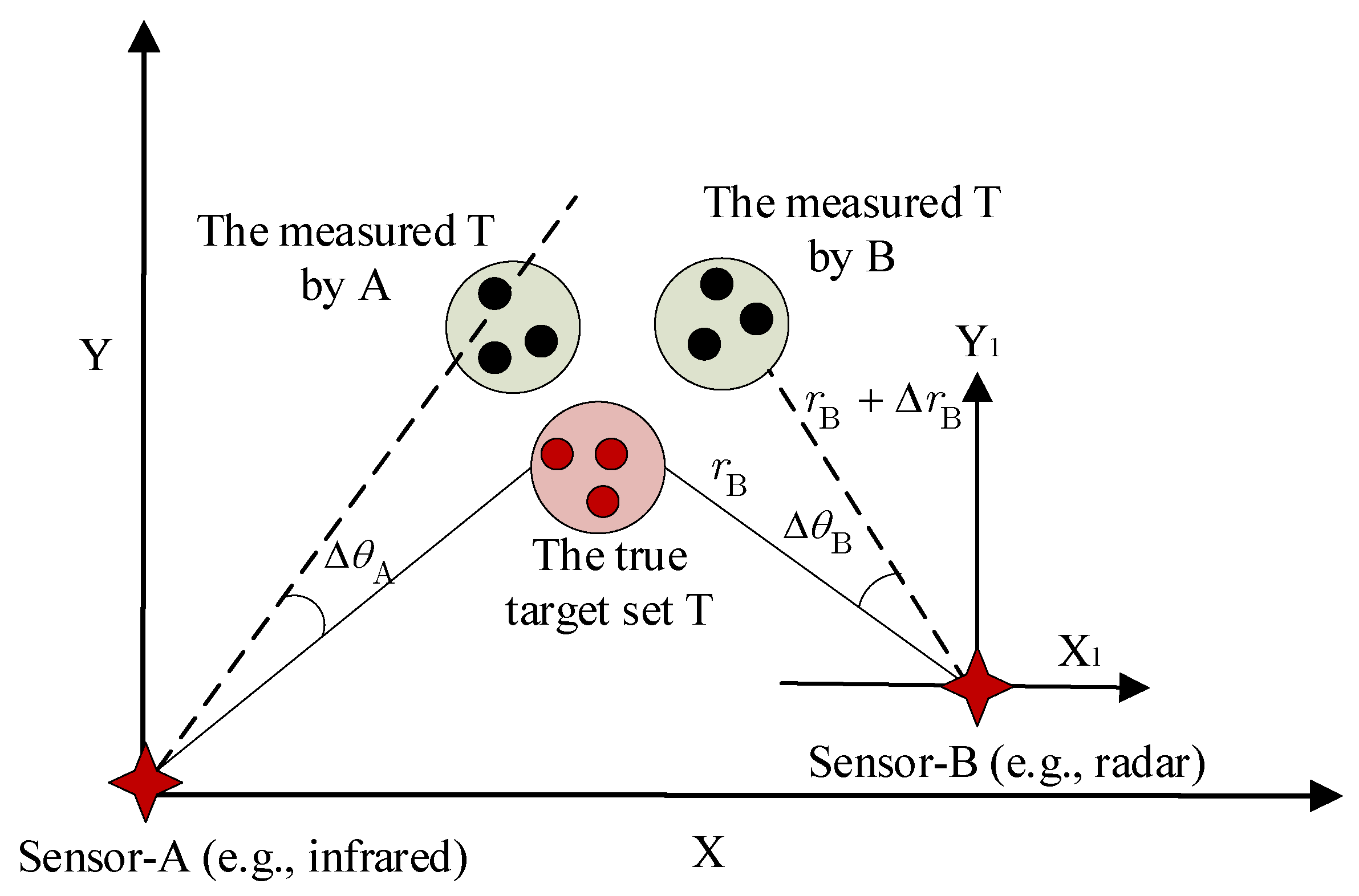
- The nonlinear relationship between the state space and measurement space in recursive filtering of heterogeneous sensors causes coupling between target states and measurement biases.
- (2)
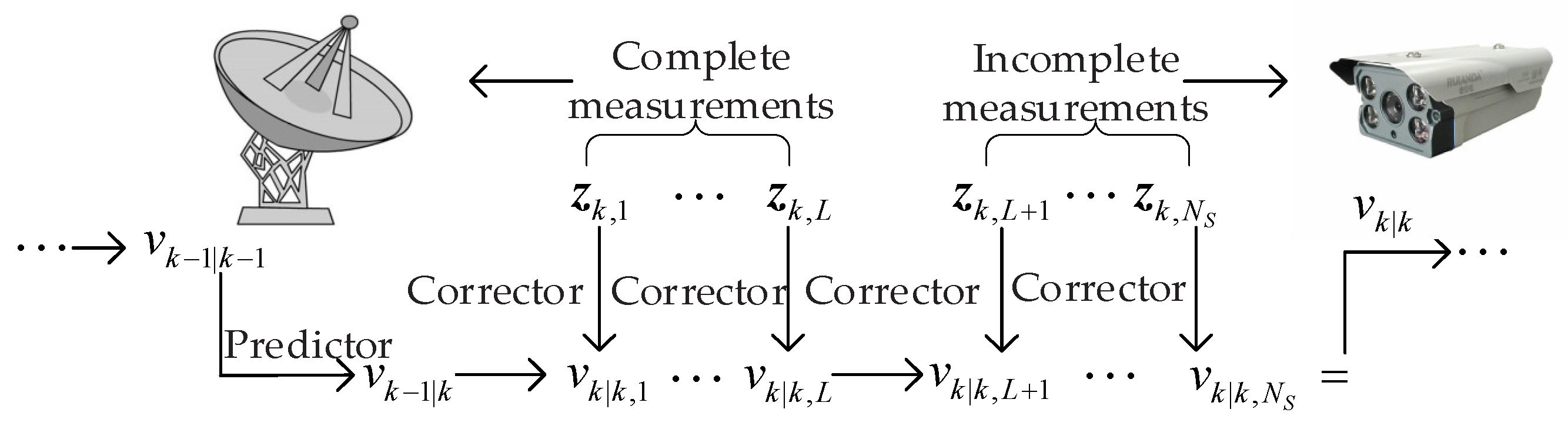
- Heterogeneous sensors yield data with varying dimensions for target detection (including complete and incomplete measurements), posing challenges for multi-sensor sequential filtering.
- (3)
- The final fusion and registration results can be affected by the varying sequential filtering order due to performance differences among sensors.
- (1)
- By constructing augmented target motion and measurement models and using PHD recursion, a closed-form expression for augmented state prediction is derived based on Gaussian mixture models. Additionally, a two-level Kalman filter is used in the update to approximately decouple the estimation of target state and measurement biases.
- (2)
- For the registration problem of heterogeneous sensors, measurements obtained from the sensors are divided into complete measurements and incomplete measurements. Sequential updates are performed first for sensors that provide complete measurements, followed by filtering updates for incomplete measurements using EKF sequential update techniques.
- (3)
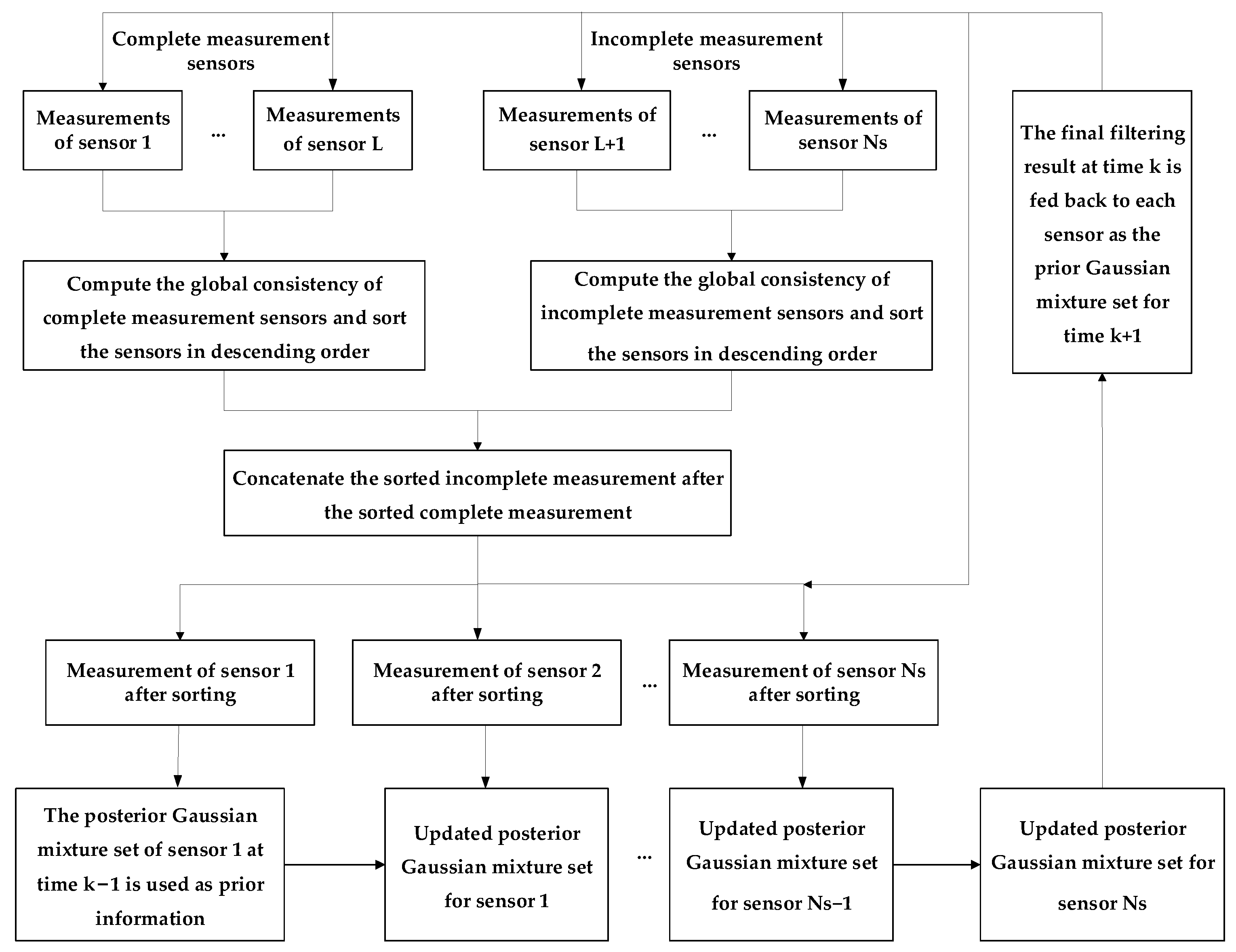
- To address the sensitivity of the sequence fusion-filtering algorithm to sensor quality differences, real-time evaluation of fusion consistency for each sensor is performed using the optimal subpattern assignment (OSPA) metric when the data quality of each sensor is unknown. By optimizing the fusion order, more accurate fusion results can be obtained.
2. Related Work
3. Problem Formulation
3.1. Linear Gaussian Dynamical Model of the Augmented State
3.2. Linear Gaussian Measurement Model of the Augmented State
3.3. Random Finite Set Formulation of Multi-Target Filtering
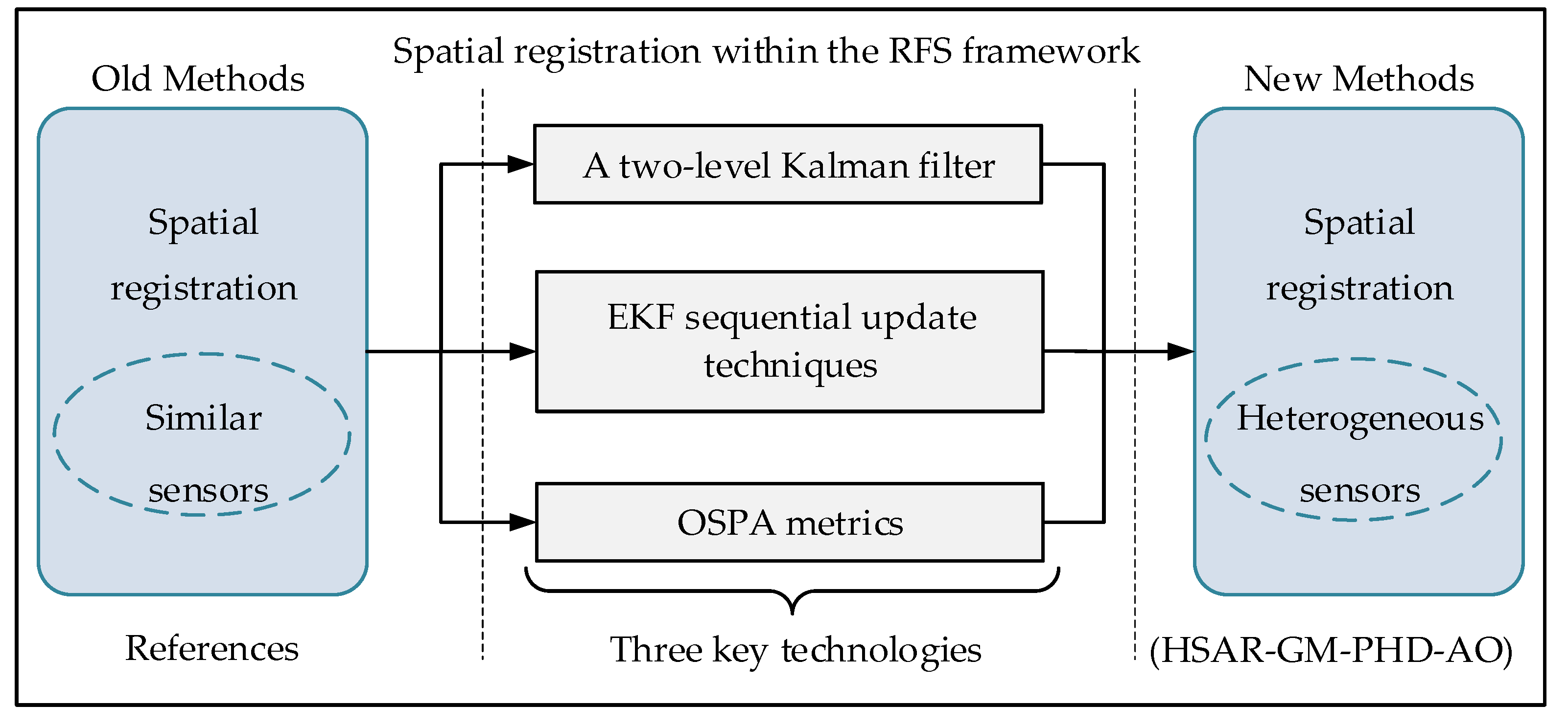
4. Methods
4.1. Augmented State GM-PHD Registration Based on Two-Level Kalman Filter
| Algorithm 1 Augmented state GM-PHD registration based on two-level Kalman filter |
| Step 1. Prediction The augmented state prediction is achieved through a two-level Kalman recursion based on Equations (26) and (27). Step 2. Update The augmented state update is achieved through a two-level Kalman recursion based on Equations (39)–(42). Step 3. Calculation of the measurement bias The measurement bias for each sensor can be achieved using Equations (45) and (46). |
4.2. Heterogeneous Multi-Sensor Sequential Filtering
4.2.1. Centralized Fusion Filtering of Heterogeneous Sensors Based on EKF
| Algorithm 2. Heterogeneous sensor registration using EKF sequential filtering |
| INPUT: , , , the number of complete measurement sensors OUTPUT: , |
| step 1. Prediction Calculate the one-step prediction state and covariance based on (29). step 2. Update the target state using complete measurements (e.g., active radar measurements).  step 3. Update the target state using incomplete measurements (e.g., infrared measurements).  step 4. Assign the filtering state estimate and covariance from incomplete measurements to the global filtering state estimate and state estimate covariance |
4.2.2. Recursive GM-PHD Filtering for Sequential Fusion with Heterogeneous Sensors
- The prediction for the target state at time is shown in Equation (22).
- Let us denote , then the equation for updating the target states with complete measurements at time can be expressed as
4.3. Heterogeneous Sensor Adaptive Measurement Iterative Update
4.3.1. Measurement Consistency Metrics
4.3.2. Iterative Update Based on Consistency Metrics
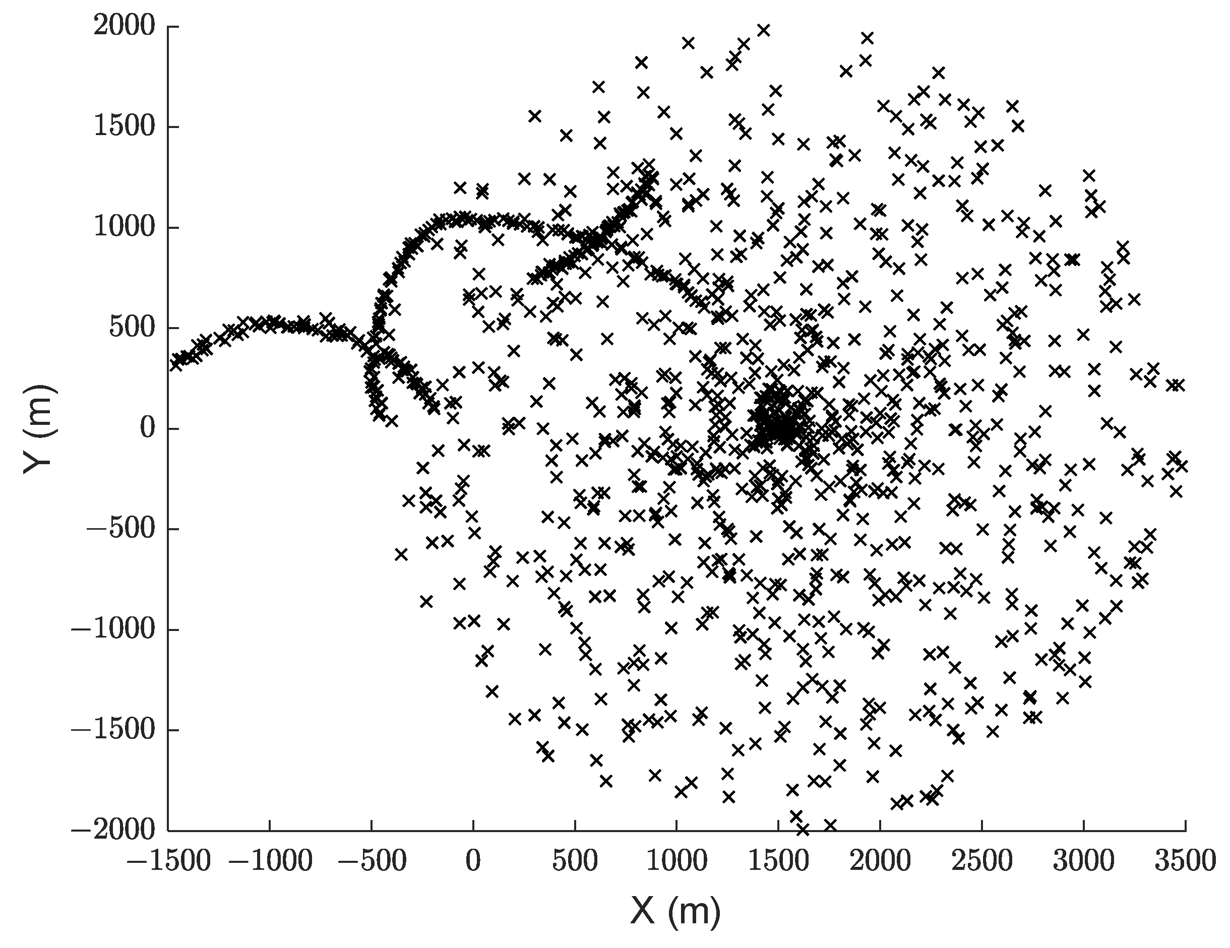
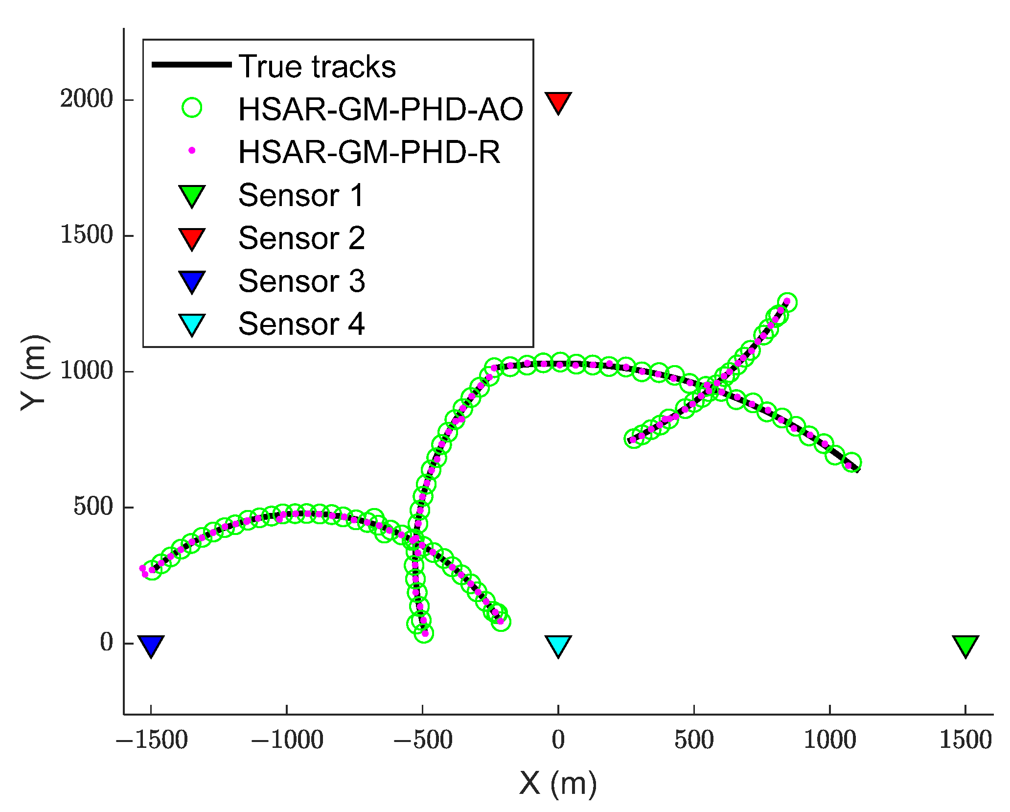
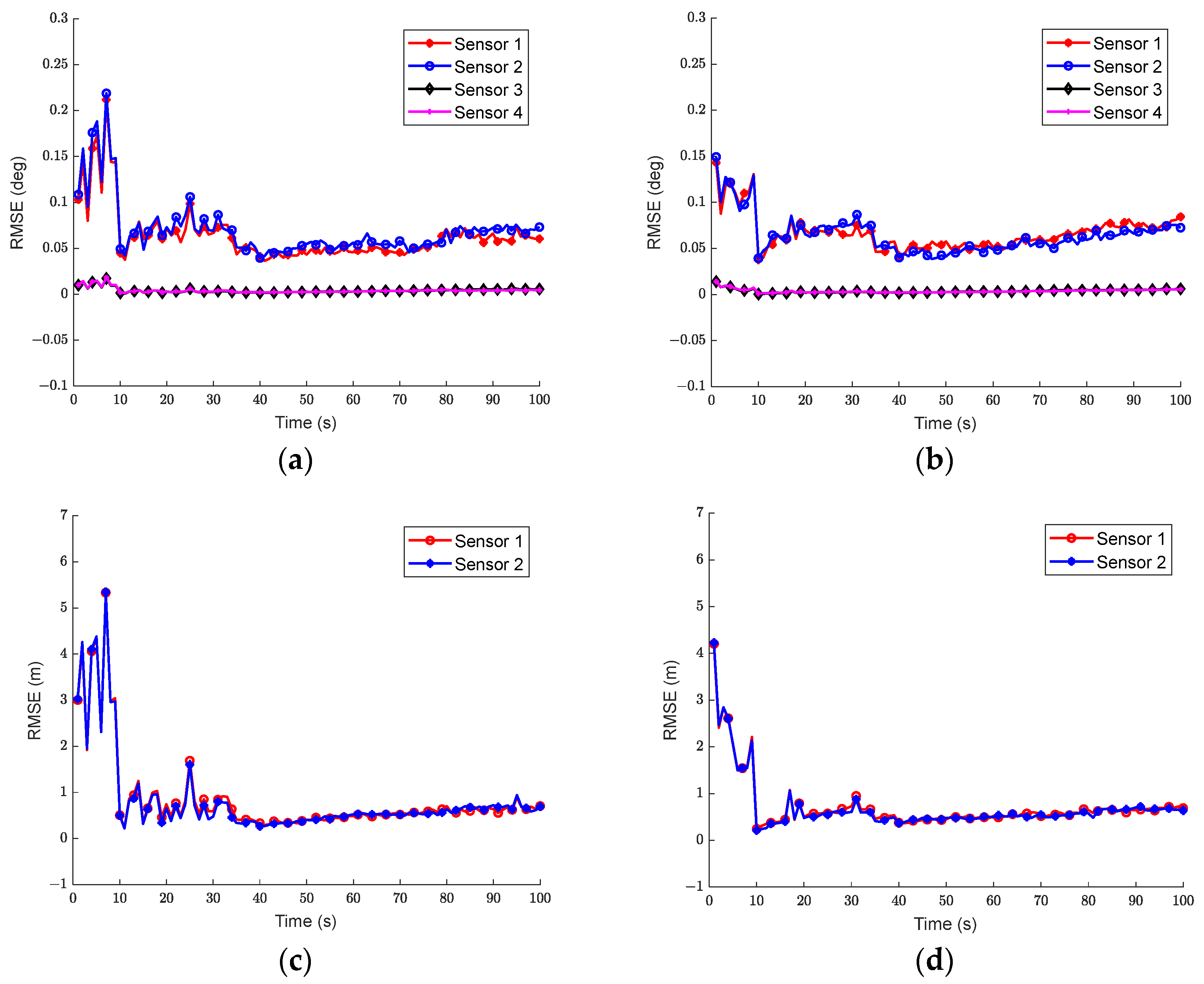
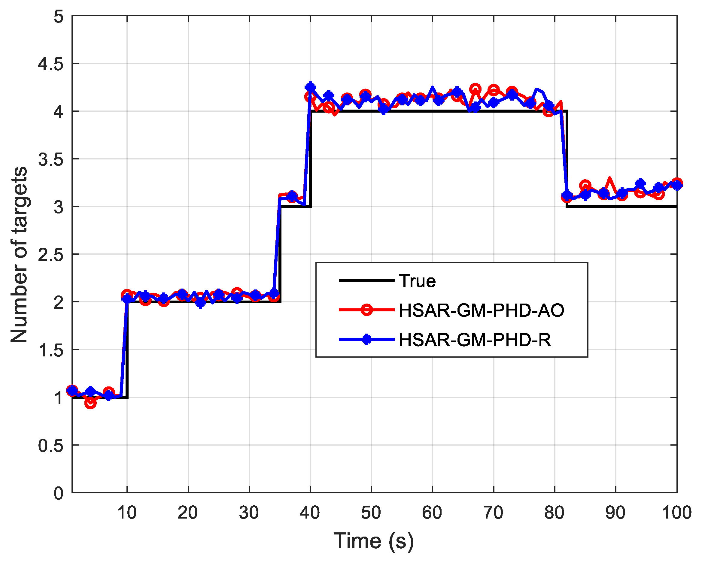
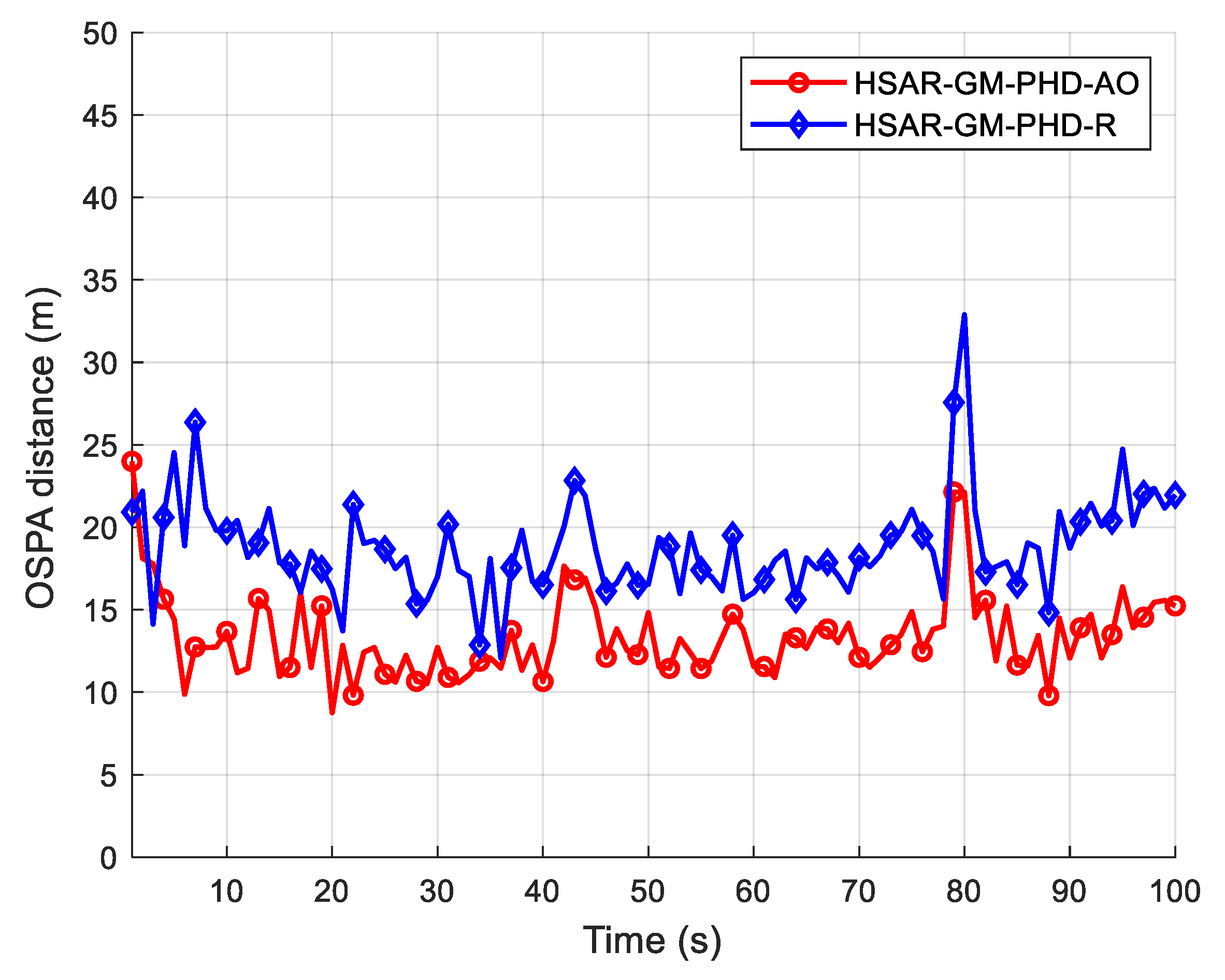
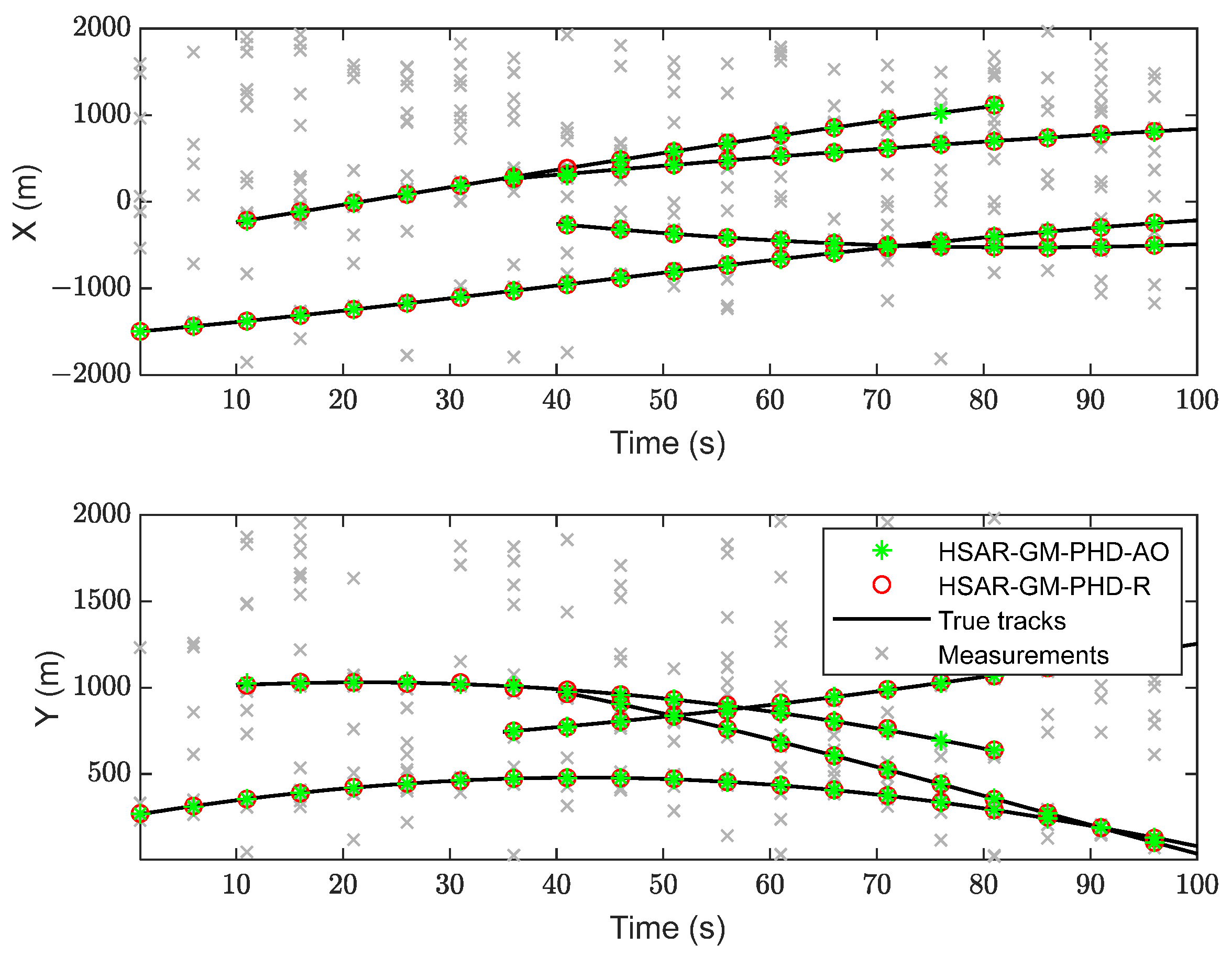
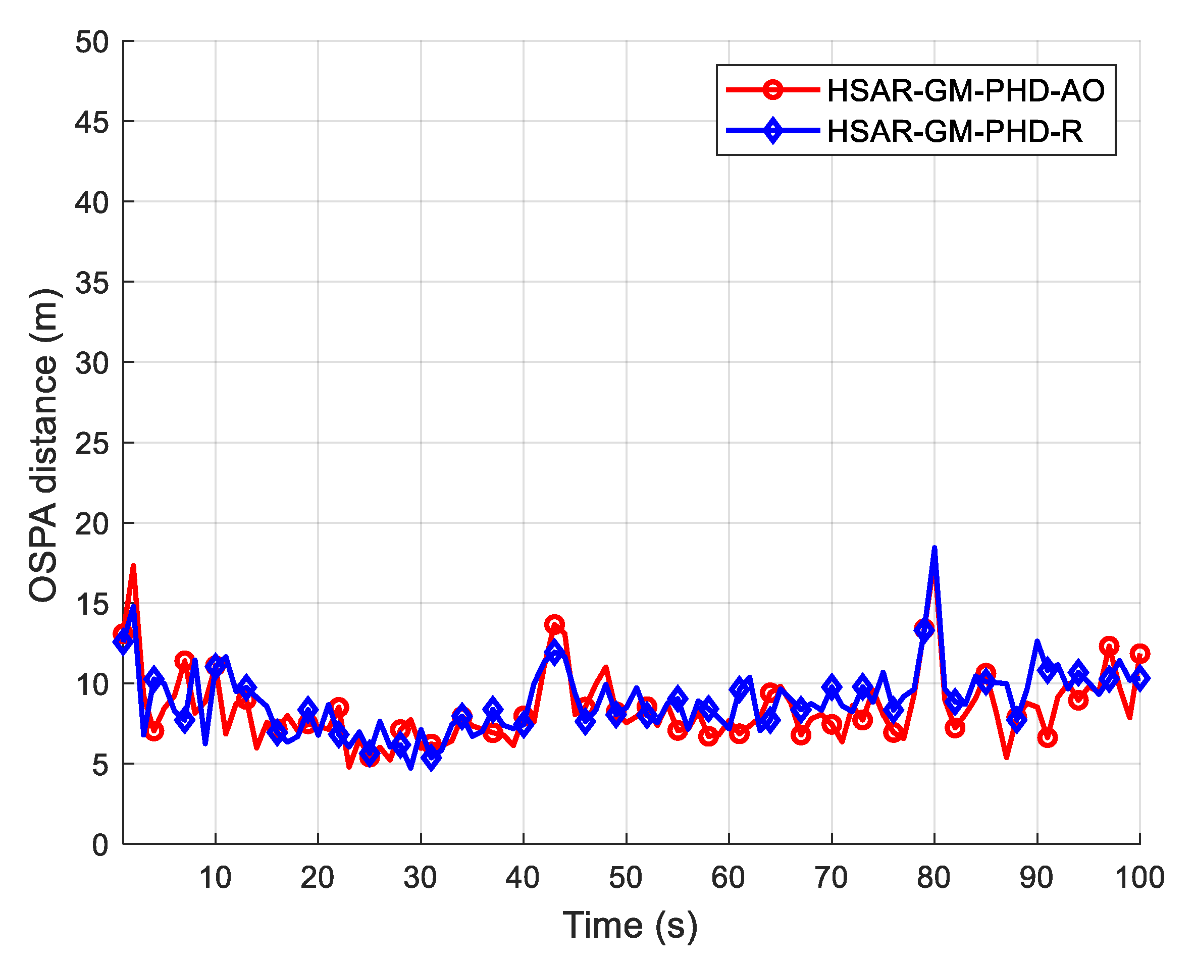
5. Experimental Results
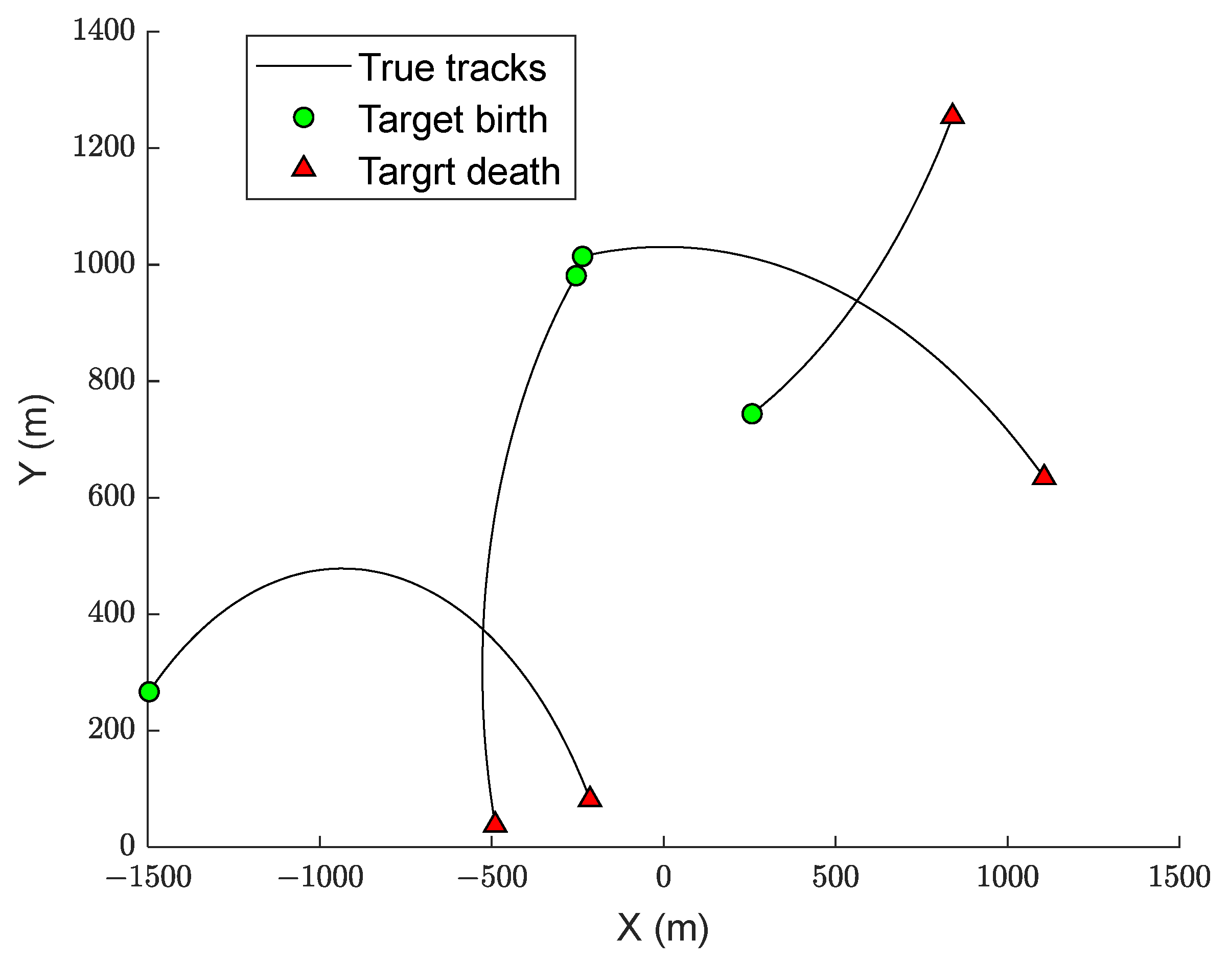
5.1. Simulation Scenarios
5.2. Simulation Results
6. Conclusions
Author Contributions
Funding
Data Availability Statement
Conflicts of Interest
Appendix A
References
- Cao, B.; Zhao, J.; Yang, P.; Yang, P.; Zhang, Y. 3-D deployment optimization for heterogeneous wireless directional sensor networks on smart city. IEEE Trans. Ind. Inform. 2018, 15, 1798–1808. [Google Scholar] [CrossRef]
- Alatise, M.B.; Hancke, G.P. A review on challenges of autonomous mobile robot and sensor fusion methods. IEEE Access 2020, 8, 39830–39846. [Google Scholar] [CrossRef]
- Li, J.; Bi, G.; Wang, X.; Nie, T.; Huang, L. Radiation-Variation Insensitive Coarse-to-Fine Image Registration for Infrared and Visible Remote Sensing Based on Zero-Shot Learning. Remote Sens. 2024, 16, 214. [Google Scholar] [CrossRef]
- Shahzad, M.K.; Islam, S.M.R.; Hossain, M.; Abdullah-Al-Wadud, M.; Alamri, A.; Hussain, M. GAFOR: Genetic Algorithm Based Fuzzy Optimized Re-Clustering in Wireless Sensor Networks. Mathematics 2021, 9, 43. [Google Scholar] [CrossRef]
- Ou, C.; Shan, C.; Cheng, Z.; Long, Y. Adaptive Trajectory Tracking Algorithm for the Aerospace Vehicle Based on Improved T-MPSP. Mathematics 2023, 11, 2160. [Google Scholar] [CrossRef]
- Bu, S.; Zhou, G. Joint data association spatiotemporal bias compensation and fusion for multisensor multitarget tracking. IEEE Trans. Signal Process. 2023, 71, 1509–1523. [Google Scholar] [CrossRef]
- Marek, J.; Chmelař, P. Survey of Point Cloud Registration Methods and New Statistical Approach. Mathematics 2023, 11, 3564. [Google Scholar] [CrossRef]
- Cormack, D.; Schlangen, I.; Hopgood, J.R.; Clark, D.E. Joint registration and fusion of an infrared camera and scanning radar in a maritime context. IEEE Trans. Aerosp. Electron. Syst. 2019, 56, 1357–1369. [Google Scholar] [CrossRef]
- Chai, L.; Yi, W.; Kong, L. Joint sensor registration and multi-target tracking with phd filter in distributed multi-sensor networks. Signal Process. 2023, 206, 108909. [Google Scholar] [CrossRef]
- Bu, S.; Kirubarajan, T.; Zhou, G. Online sequential spatiotemporal bias compensation using multisensor multitarget measurements. Aerosp. Sci. Technol. 2021, 108, 106407. [Google Scholar] [CrossRef]
- Mahler, R. Advances in Statistical Multi-Source Multi-Target Information Fusion; Artech House: Norwood, MA, USA, 2014. [Google Scholar]
- Mahler, R. PHD Filters of Higher Order in Target Number. IEEE Trans. Aerosp. Electron. Syst. 2007, 43, 1523–1543. [Google Scholar] [CrossRef]
- Mahler, R. Multitarget Bayes filtering via first-order multitarget moments. IEEE Trans. Aerosp. Electron. Syst. 2003, 39, 1152–1178. [Google Scholar] [CrossRef]
- Vo, B.N.; Singh, S.; Doucet, A. Sequential Monte Carlo methods for multi-target filtering with random finite sets. IEEE Trans. Aerosp. Electron. Syst. 2005, 41, 1224–1245. [Google Scholar]
- Vo, B.N.; Singh, S.; Doucet, A. Sequential Monte Carlo implementation of the PHD filter for multi-target tracking. In Proceedings of the 6th International Conference on Information Fusion, Cairns, Australia, 8–11 July 2003; pp. 792–799. [Google Scholar]
- Vo, B.N.; Ma, W.K. The Gaussian mixture probability hypothesis density filter. IEEE Trans. Signal Process. 2006, 54, 4091–4104. [Google Scholar] [CrossRef]
- Clark, D.E.; Vo, B.N. Convergence analysis of the Gaussian mixture PHD filter. IEEE Trans. Signal Process. 2007, 55, 1204–1211. [Google Scholar] [CrossRef]
- Shi, K.; Shi, Z.; Yang, C.; He, S.; Chen, J.; Chen, A. Road-Map Aided GM-PHD Filter for Multivehicle Tracking with Automotive Radar. IEEE Trans. Ind. Inform. 2022, 18, 97–108. [Google Scholar] [CrossRef]
- Sung, Y.; Tokekar, P. GM-PHD Filter for Searching and Tracking an Unknown Number of Targets with a Mobile Sensor with Limited FOV. IEEE Trans. Autom. Sci. Eng. 2022, 19, 2122–2134. [Google Scholar] [CrossRef]
- Mahler, R. The Multisensor PHD filter: II. Erroneous Solution via “Poisson magic”. In Signal Processing, Sensor Fusion, and Target Recognition; International Society for Optics and Photonics: Orlando, FL, USA, 2009; pp. 182–193. [Google Scholar]
- VO, B.T.; See, C.M.; Ma, N.; Ng, W.T. Multi-sensor joint detection and tracking with the Bernoulli filter. IEEE Trans. Aerosp. Electron. Syst. 2012, 48, 1385–1402. [Google Scholar] [CrossRef]
- Liu, L.; Ji, H.; Fan, Z. Improved Iterated-corrector PHD with Gaussian mixture implementation. Signal Process. 2015, 114, 89–99. [Google Scholar] [CrossRef]
- Lian, F.; Han, C.; Liu, W.; Chen, H. Joint spatial registration and multitarget tracking using an extended probability hypothesis density filter. IET Radar Sonar Navig. 2011, 5, 441–448. [Google Scholar] [CrossRef]
- Li, W.; Jia, Y.; Du, J.; Yu, F. Gaussian mixture PHD filter for multi-sensor multi-target tracking with registration errors. Signal Process. 2013, 93, 86–99. [Google Scholar] [CrossRef]
- Wu, W.; Jiang, J.; Liu, W.; Feng, X.; Gao, L.; Qin, X. Augmented state GM-PHD filter with registration errors for multi-target tracking by Doppler radars. Signal Process. 2016, 120, 117–128. [Google Scholar] [CrossRef]
- Fortunati, S.; Farina, A.; Gini, F.; Graziano, A.; Greco, M.S.; Giompapa, S. Least squares estimation and cramer–rao type lower bounds for relative sensor registration process. IEEE Trans. Signal Process. 2010, 59, 1075–1087. [Google Scholar] [CrossRef]
- Rhode, S.; Usevich, K.; Markovsky, I.; Gauterin, F. A recursive restricted total least-squares algorithm. IEEE Trans. Signal Process. 2014, 62, 5652–5662. [Google Scholar] [CrossRef]
- Pulford, G.W. Analysis of a nonlinear least squares procedure used in global positioning systems. IEEE Trans. Signal Process. 2010, 58, 4526–4534. [Google Scholar] [CrossRef]
- Bai, S.; Zhang, Y. Error registration of netted radar by using GLS algorithm. In Proceedings of the 33rd Chinese Control Conference, Nanjing, China, 28–30 July 2014; pp. 7430–7433. [Google Scholar]
- Zhou, Y.; Leung, H.; Blanchette, M. Sensor alignment with earth-centered earth-fixed (ECEF) coordinate system. IEEE Trans. Aerosp. Electron. Syst. 1999, 35, 410–418. [Google Scholar] [CrossRef]
- Lu, C.; Wang, X.; Koutsoukos, X. Feedback utilization control in distributed real-time systems with end-to-end tasks. IEEE Trans. Parall. Distr. Syst. 2005, 16, 550–561. [Google Scholar]
- Zhou, Y.F.; Leung, H.; Yip, P.C. An exact maximum likelihood registration algorithm for data fusion. IEEE Trans. Signal Process. 1997, 45, 1560–1573. [Google Scholar] [CrossRef]
- Chitour, Y.; Pascal, F. Exact Maximum Likelihood Estimates for SIRV Covariance Matrix: Existence and Algorithm Analysis. IEEE Trans. Signal Process. 2008, 56, 4563–4573. [Google Scholar] [CrossRef]
- Okello, N.; Ristic, B. Maximum likelihood registration for multiple dissimilar sensors. IEEE Trans. Aerosp. Electron. Syst. 2003, 39, 1074–1083. [Google Scholar] [CrossRef]
- Wang, J.; Zeng, Y.; Wei, S.; Wei, Z.; Wu, Q.; Savaria, Y. Multisensor track-to-track association and spatial registration algorithm under incomplete measurements. IEEE Trans. Signal Process. 2021, 69, 3337–3350. [Google Scholar] [CrossRef]
- Ristic, B.; Clark, D.; Gordon, N. Calibration of multi-target tracking algorithms using non-cooperative targets. IEEE J. Sel. Top. Signal Process. 2013, 7, 390–398. [Google Scholar] [CrossRef]
- Ristic, B.; Clark, D. Particle filter for joint estimation of multi-target dynamic state and multi-sensor bias. In Proceedings of the IEEE International Conference on Acoustics, Speech, and Signal Processing, Kyoto, Japan, 25–30 March 2012; pp. 3877–3880. [Google Scholar]
- Yi, W.; Li, G.; Battistelli, G. Distributed Multi-Sensor Fusion of PHD Filters with Different Sensor Fields of View. IEEE Trans. Signal Process. 2020, 68, 5204–5218. [Google Scholar] [CrossRef]
- Liu, S.; Shen, H.; Chen, H.; Peng, D.; Shi, Y. Asynchronous Multi-Sensor Fusion Multi-Target Tracking Method. In Proceedings of the 14th International Conference on Control and Automation, Anchorage, AK, USA, 12–15 June 2018; pp. 459–463. [Google Scholar]
- Tollkühn, A.; Particke, F.; Thielecke, J. Gaussian state estimation with non-gaussian measurement noise. In Proceedings of the Sensor Data Fusion: Trends, Solutions, Applications (SDF), Bonn, Germany, 9–11 October 2018; pp. 1–5. [Google Scholar]
- Bar-Shalom, Y.; Willett, P.K.; Tian, X. Tracking and Data Fusion; YBS Publishing: Storrs, CT, USA, 2011. [Google Scholar]
- Taghavi, E.; Tharmarasa, R.; Kirubarajan, T.; Bar-Shalom, Y.; Mcdonald, M. A practical bias estimation algorithm for multisensor-multitarget tracking. IEEE Trans. Aerosp. Electron. Syst. 2016, 52, 2–19. [Google Scholar] [CrossRef]
- Wang, R.; Mao, H.; Hu, C.; Zeng, T.; Long, T. Joint association and registration in a multiradar system for migratory insect track observation. IEEE Trans. Aerosp. Electron. Syst. 2021, 57, 4028–4043. [Google Scholar] [CrossRef]


| Target Number | Initial State | Survival Time |
|---|---|---|
| 1 | ||
| 2 | ||
| 3 | ||
| 4 |
| Sensor Number | Sensor State | Biases | Observation Time |
|---|---|---|---|
| 1 | |||
| 2 | |||
| 3 | |||
| 4 |
| Gaussian Component | |
|---|---|
| 1 | |
| 2 | |
| 3 | |
| 4 |
| Scenario | Detection Probability | Clutter Intensity |
|---|---|---|
| 1 | ||
| 2 | ||
| 3 | ||
| 4 |
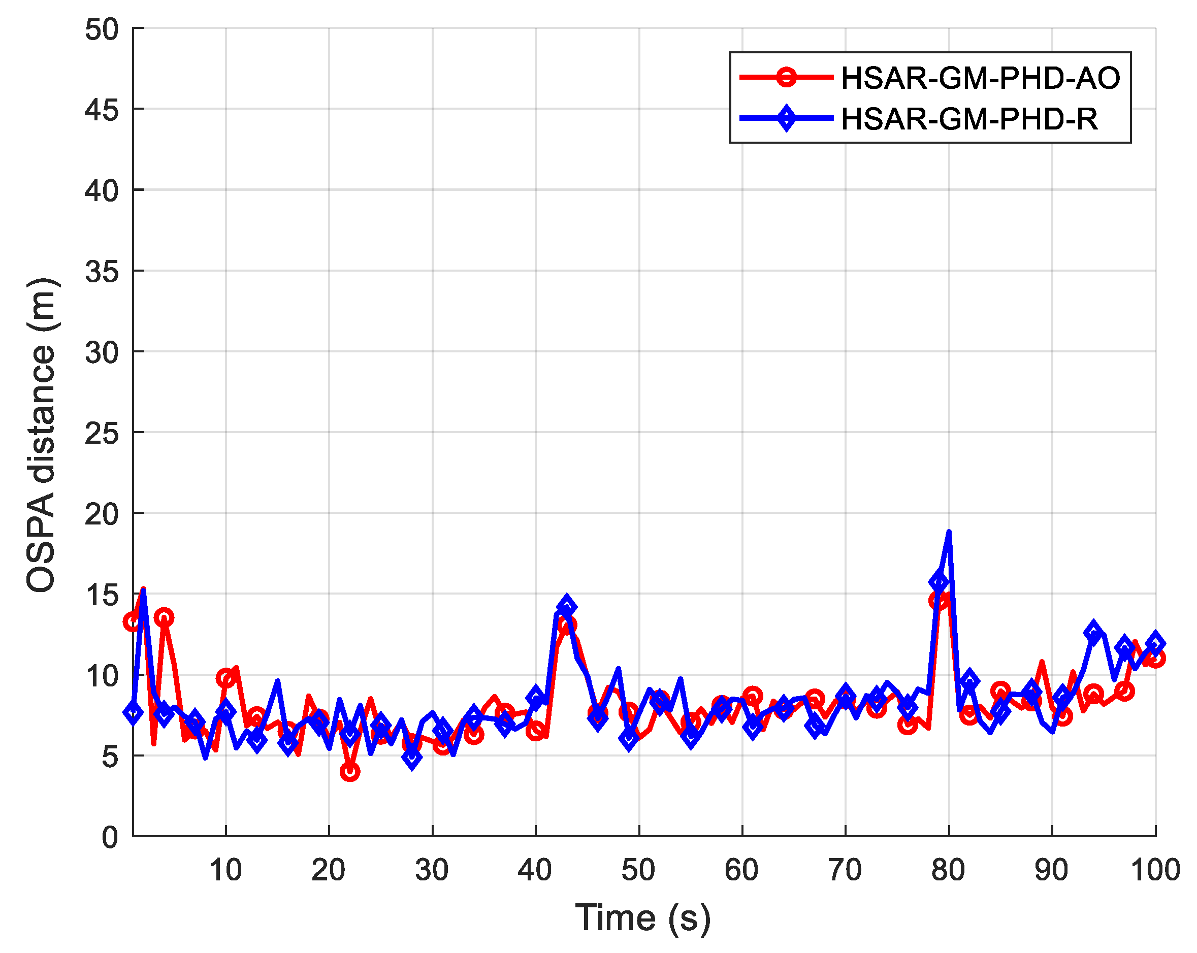
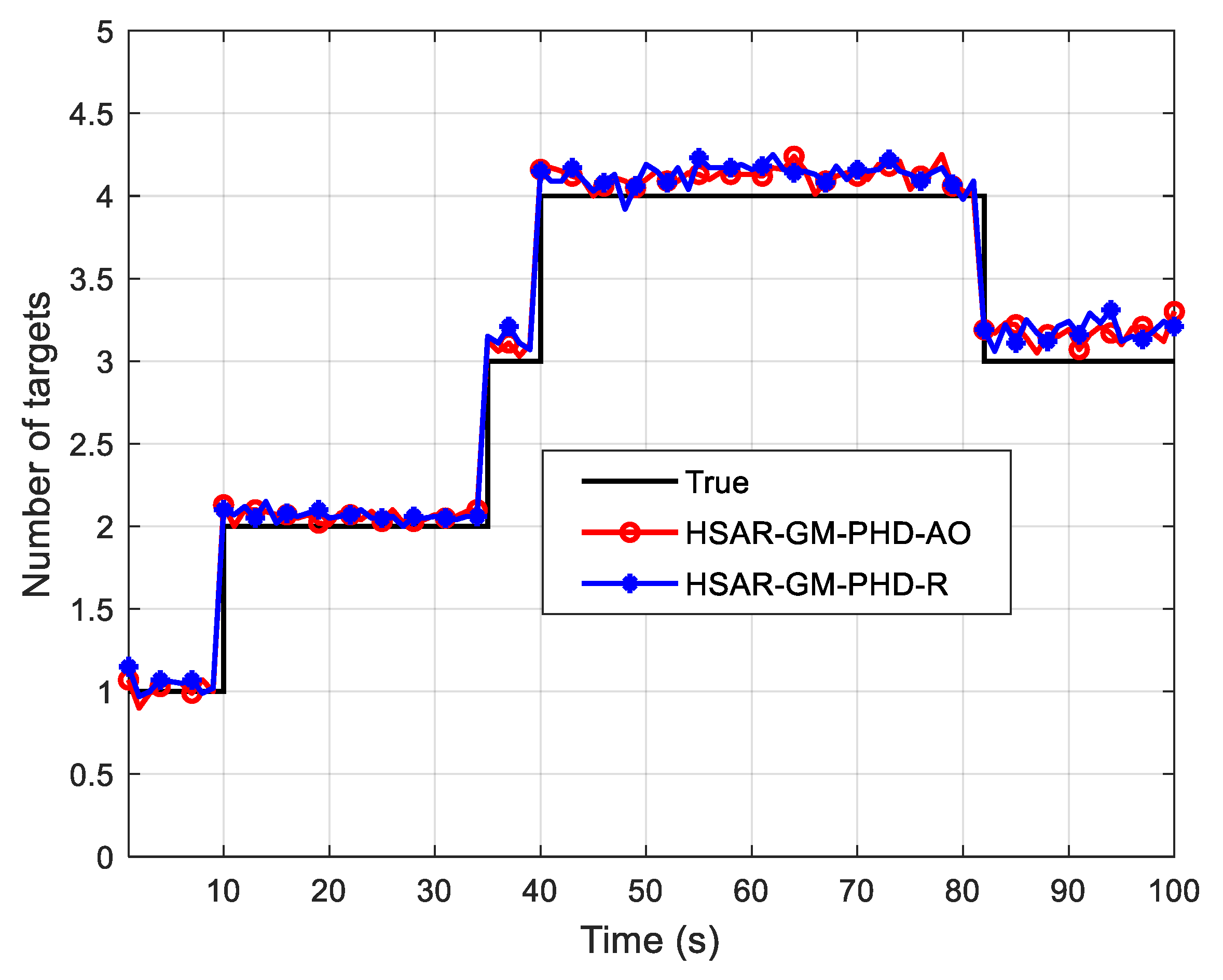
| Algorithm | Average OSPA Distance from 40 s and 80 s | Average Target Cardinality Estimation from 40 s and 80 s |
|---|---|---|
| HSAR-GM-PHD-AO | 8.84 | 4.08 |
| HSAR-GM-PHD-R | 8.89 | 4.11 |
| Algorithm | Average OSPA Distance from 40 s and 80 s | Average Target Cardinality Estimation from 40 s and 80 s |
|---|---|---|
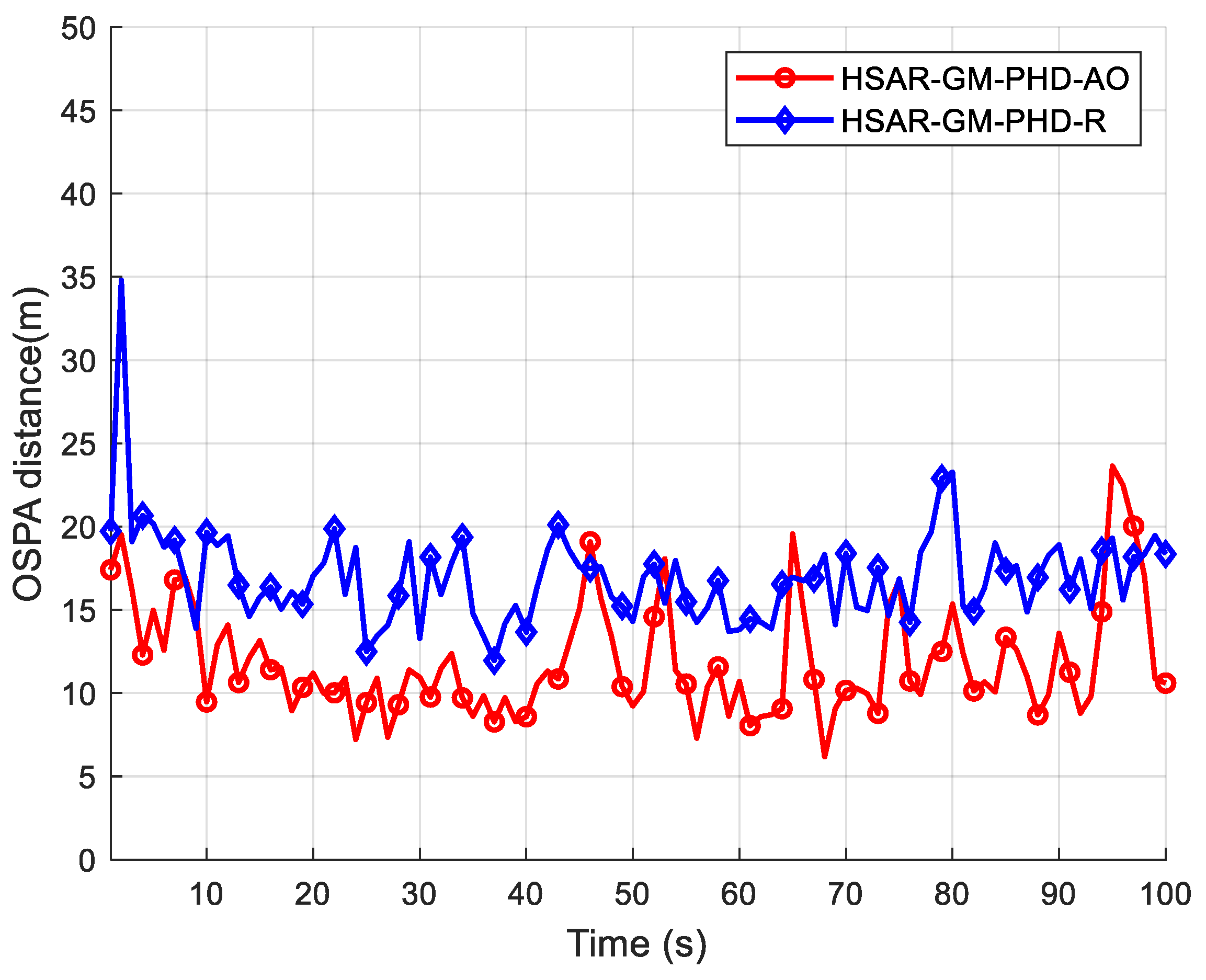
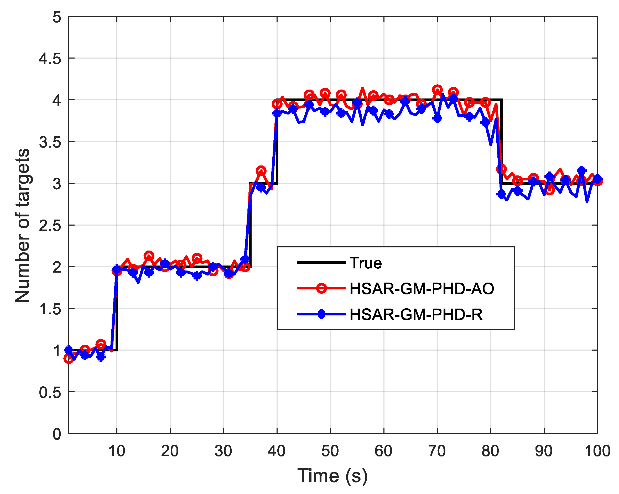
| HSAR-GM-PHD-AO | 11.23 | 4.12 |
| HSAR-GM-PHD-R | 16.57 | 4.21 |
| Algorithm | Average OSPA Distance from 40 s and 80 s | Average Target Cardinality Estimation from 40 s and 80 s |
|---|---|---|
| HSAR-GM-PHD-AO | 8.48 | 4.13 |
| HSAR-GM-PHD-R | 8.85 | 4.13 |
| Algorithm | Average OSPA Distance from 40 s and 80 s | Average Target Cardinality Estimation from 40 s and 80 s |
|---|---|---|
| HSAR-GM-PHD-AO | 11.58 | 4.05 |
| HSAR-GM-PHD-R | 17.72 | 3.81 |
| Sensor Number | Rate (%) | Observation Environment | ||
|---|---|---|---|---|
| θ | R | Detection Probability | Clutter Intensity | |
| S1 | 7.2 | 10.5 | ||
| S2 | 9.7 | 13.1 | ||
| S3 | 7.4 | |||
| S4 | 10.1 | |||
| Average | 8.6 | 11.8 | ||
Disclaimer/Publisher’s Note: The statements, opinions and data contained in all publications are solely those of the individual author(s) and contributor(s) and not of MDPI and/or the editor(s). MDPI and/or the editor(s) disclaim responsibility for any injury to people or property resulting from any ideas, methods, instructions or products referred to in the content. |
© 2024 by the authors. Licensee MDPI, Basel, Switzerland. This article is an open access article distributed under the terms and conditions of the Creative Commons Attribution (CC BY) license (https://creativecommons.org/licenses/by/4.0/).
Share and Cite
Zeng, Y.; Wang, J.; Wei, S.; Zhang, C.; Zhou, X.; Lin, Y. Gaussian Mixture Probability Hypothesis Density Filter for Heterogeneous Multi-Sensor Registration. Mathematics 2024, 12, 886. https://doi.org/10.3390/math12060886
Zeng Y, Wang J, Wei S, Zhang C, Zhou X, Lin Y. Gaussian Mixture Probability Hypothesis Density Filter for Heterogeneous Multi-Sensor Registration. Mathematics. 2024; 12(6):886. https://doi.org/10.3390/math12060886
Chicago/Turabian StyleZeng, Yajun, Jun Wang, Shaoming Wei, Chi Zhang, Xuan Zhou, and Yingbin Lin. 2024. "Gaussian Mixture Probability Hypothesis Density Filter for Heterogeneous Multi-Sensor Registration" Mathematics 12, no. 6: 886. https://doi.org/10.3390/math12060886
APA StyleZeng, Y., Wang, J., Wei, S., Zhang, C., Zhou, X., & Lin, Y. (2024). Gaussian Mixture Probability Hypothesis Density Filter for Heterogeneous Multi-Sensor Registration. Mathematics, 12(6), 886. https://doi.org/10.3390/math12060886