Optimizing Ensemble Learning to Reduce Misclassification Costs in Credit Risk Scorecards

Abstract

Credit risk scorecard models are utilized by lending institutions to optimize decisions on credit approvals. In recent years, ensemble learning has often been deployed to reduce misclassification costs in credit risk scorecards. In this paper, we compared the risk estimation of 26 widely used machine learning algorithms based on commonly used statistical metrics. The best-performing algorithms were then used for model selection in ensemble learning. For the first time, we proposed financial criteria that assess the impact of losses associated with both false positive and false negative predictions to identify optimal ensemble learning. The German Credit Dataset (GCD) is augmented with simulated financial information according to a hypothetical mortgage portfolio observed in UK, European and Australian banks to enable the assessment of losses arising from misclassification costs. The experimental results using the simulated GCD show that the best predictive individual algorithm with the accuracy of 0.87, Gini of 0.88 and Area Under the Receiver Operating Curve of 0.94 was the Generalized Additive Model (GAM). The ensemble learning method with the lowest misclassification cost was the combination of Random Forest (RF) and K-Nearest Neighbors (KNN), totaling USD 417 million in costs (USD 230 for default costs and USD 187 for opportunity costs) compared to the costs of the GAM (USD 487, USD 287 and USD 200). Implementing the proposed financial criteria has led to a significant USD 70 million reduction in misclassification costs derived from a small sample. Thus, the lending institutions’ profit would considerably rise as the number of submitted credit applications for approval increases.

1. Introduction

Lending is an essential part of the monetary economy that facilitates both stability and growth of the financial system [1]. Because of the risk of loss in lending to customers, financial institutions perform assessments using credit scorecards. Supervised learning techniques are usually deployed for this purpose, seeking to associate historical customer characteristics with default to estimate the probability that a future applicant will default [2]. This scoring approach forms the basis for acceptance or rejection of credit in modern lending practices, particularly as applied to retail lending portfolios.

The decision criteria to lend to an applicant must be sufficiently robust to reject potential defaulters as well as flexible enough to maintain a sufficient volume of good customers to be profitable. Approving customers who eventually default can be enormously costly while rejecting customers who will not default can also put a lending business at risk due to failing to make enough profit. The costs associated with wrongly approving or rejecting customers are referred to as misclassification costs.

Traditionally machine learning approaches are utilized to make credit application decisions. Optimizing the quality of lending decisions through deploying the most robust models has a tangible benefit on the ability of credit providers to be sufficiently profitable in an intensely competitive environment. Evidence suggests that combining machine learning algorithms into ensemble models may further improve the quality of credit approvals and drive down misclassification costs. The main motivation for this paper is to seek to improve the quality of credit risk decisions by developing, identifying and deploying the best possible predictive system.

A great deal of prior research has been performed seeking to identify superior learning algorithms and model performance measures (for example, refs. [3,4]) in credit scoring. Moreover, there has been a long-standing interest in improving the strength of predictive methods by hybridizing models in credit risk, employing techniques such as rescoring rejected applicants to reduce Type I errors [5], combining bespoke models with external bureau type models [6] and two-stage approaches, such as first clustering and then using a neural network to classify the clusters [7]. Indeed, researchers continue to evaluate a wide variety of bespoke ensemble methods for credit scoring in pursuit of optimal credit risk assessment (for example, refs. [8,9,10,11]).

The term “ensemble learning” can be applied to homogeneous collections of models that are minor variations of the same model [12], and also hybridized models that are not from the same family, or so-called heterogeneous collections. We use the term “ensemble learning” to describe an approach in which two or more models are fitted to the same data and the predictions of each model are combined.

Ensemble learning can be achieved in three different ways: boosting, bagging or stacking. Boosting trains base learners such that weak learners are converted into strong learners on sequential samples and data are generated for each new base learner to target the errors made by previous base learners [13]. In contrast, bagging selects several different training sets using a bootstrapped process, and the algorithm is trained on each sample before the final model is obtained by voting (in classification models) [14]. The third approach, and the focus of this paper, known as stacking, was first proposed by [15] in application to neural networks and later extended to numeric prediction by [16]. Stacking [15], also called meta ensembling or stacked generalization, is a well-known method used to increase diversity and generalization. Using multiple learners, stacking aggregates each model in a tiered structure. More precisely, the process of stacking is to build multiple classifiers in the first layer to form a base-level learner. Then, the output of this layer is taken as a new feature to re-train a new learner, the meta-level learner.

The results of comparing the performance of various models by scholars show that different stacking approaches perform better than individual algorithms [17], and modelers usually observe better predictive performance by aggregating predictions compared to only a single algorithm [18]. In the context of ensemble learning regression, it has been shown that, if the stacking model is properly combined, the squared error of the prediction can be smaller than the average squared error of the base learners [19]. However, there are only a few researchers seeking to evaluate different approaches to ensemble models for credit risk under financial performance criteria [20].

In this paper, for the first time, we expand model evaluation for the selection process considering two broad classes of performance metrics: classical statistical metrics, which are typically observed in credit risk modeling, including Gini, accuracy and Area Under the Receiver Operating Curve (AUC), as well as financial criteria to determine the financial impact of losses associated with false predictions. We simulated financial variables according to a hypothetical mortgage portfolio aligned with the scale of similar asset classes observed in banks in Australia, the UK and Europe. These were appended to the German Credit Dataset (GCD). Using the simulated data, the risk estimations of 26 widely used machine learning algorithms based on commonly used statistical metrics [2,3,4,7,10] were compared. The best-performing algorithms were selected for ensemble learning. This is followed by employing the proposed financial criteria to develop the optimal ensemble learning. The results of our experiments demonstrate that the Generalized Additive Model (GAM) is the best predictive individual algorithm, and the optimal ensemble learning containing K-Nearest Neighbors (KNN) and Random Forest (RF) achieves the lowest misclassification cost.

Including a larger number of financial variables in the research would improve both the diversity and the sample size, which is a limitation of the current study and may provide a more robust predictive model. In addition, replacing the simulated variables with real-time measurements may serve to further underscore the value of the financial performance metric across different types of risks with different magnitudes.

2. Methods

This section presents a brief overview of the algorithms that were applied to GCD [21] seeking to optimally predict credit risk. A wide variety of algorithms are considered, including parametric and non-parametric models. Non-parametric models are often utilized as comparison models in the industry for validation and, given their simpler formulation, would therefore be much more desirable than the usual parametric methods if they can be shown to outperform or even approximate the performance achieved using more complex models.

As ensemble models typically work best when algorithms have uncorrelated error structures, we utilized 26 classification algorithms comprising a wide variety of analytical philosophies. All modeling was performed in R (v1.7.7.1). In selecting candidate algorithms, consideration was also given to availability under the Caret package, which enables the same model-building process for each different approach.

2.1. Linear Models

Logistic Regression (LR) [22] is a process of modeling the probability of class membership of a binary outcome (although can be used for multinomial problems as well). It extends linear regression using the classical sigmoid function such that rather than an infinite continuous output, all predicted values fall between 0 and 1 (a feature found in many different approaches to classification modeling). Generalized Additive Models (GAM) [23] relax the assumptions of the classic Generalized Linear Model.

Linear Discriminant Analysis (LDA) is a dimensionality reduction technique that seeks to project data onto a hyperplane in order to maximize classes’ separability and reduce the variation between each category [24]. Naive Bayes (NB) seeks to classify instances based on the probabilities of previously seen variables, assuming complete attribute independence [25]. Partial Least Squares (PLS) regression identifies principal components that not only summarize the original predictors but are also related to the outcome [26]. These components are then used to fit the regression model. Quadratic Discriminant Analysis (QDA) is an extension of LDA. Unlike LDA, QDA considers each class to have its own variance or covariance matrix rather than having a common one [24].

Multi-Adaptive Regression Splines (MARS) [27] is an expansion in product spline basis functions, where the number of basis functions as well as the parameters associated with each one (product degree and knot locations) are determined by the algorithm. This procedure is similar to recursive partitioning approaches such as CART and shares its ability to capture high-order interactions, yet it has more power and flexibility to model relationships that are nearly additive or involve interactions in at most a few variables. A Generalized Linear Model Network (GLMn) fits generalized linear and similar models via penalized maximum likelihood. This is achieved by computing a regularization path for the lasso or an elastic net penalty at a grid of values for the regularization parameter [28].

2.2. Non-Parametric Models

The C5.0 algorithm (C5.0) is a rule-based decision tree that uses the entropy or purity of a class to decide on which features to split. This implementation extends the C4.5 classification algorithms described in [29]. The Distance-Weighted Discrimination Polynomial (DWDp) classifies data into two distinct subsets by finding a hyperplane between the two sets of points using polynomial embedding [30]. Polynomial embedding adds additional features to differentiate between hyperplanes, particularly where there is a departure from Gaussianity, and provides a simple solution to data transformation so that separating hyperplanes becomes useful.

K-Nearest Neighbors (KNN) uses proximity to make classifications or predictions about the grouping of an individual data point [31]. Recursive Partitioning and Decision Trees (RPAR) are used to determine a nested sequence of subtrees by recursively snipping off the least important splits, based on a complexity parameter [32].

2.3. Bagging Models

Random Forest (RF) constructs multiple decision trees to reach a single result, which is achieved through voting [33]. Boosted Multi-Adaptive Regression Splines (BMARS) is an implementation of MARS that also incorporates a homogeneous bagging element [31]. Conditional RF (CRF) is an implementation of RF that applies the classical RF bagging ensemble approach to conditional inference trees as base learners [34].

2.4. Boosting Models

The AdaBoost (ADAB) algorithm [35] adds weak variables sequentially using weighted training data. Predictions are made by calculating the weighted average of the weak classifiers. Additive Logistic Regression (ADA) fits stochastic boosting models for a binary response as described by Friedman et al. [36]. The Gradient Boosting Machine (GBM) trains many models in a gradual, additive and sequential manner and identifies weak learners using gradients in a loss function [37].

Extreme Gradient Boosting (XGB), proposed by Chen and Guestrin [38], offers many enhancements over the GBM including regularization and parallel processing. Yuam’s [39] R package provides two different implementations of the XGB algorithm considered here, including XGBt, which applies a gradient boosting framework using a tree learning algorithm and XGBl, which applies a gradient boosting framework using a linear model solver.

2.5. Neural Models

Multilayer Perceptron (MLP) uses fully connected feed-forward networks and is probably the most common network architecture in use. Training is performed by error backpropagation [40]. Deep Neural Networks (DNNs) are custom deep neural networks that customize the neural network to a maximal degree using an MLP as their base. Multilayer Perceptron Machine Learning (MLPm) is another variant of MLP that allows multiple layers (in addition to the standard single hidden layer) and tuning of each layer individually [40].

Multi-Step Adaptive Elastic-Net (MSAe) [41] is an algorithm for feature selection in high-dimensional regressions. Support Vector Machine with Radial Basis Function (SVMr) uses a kernel method, which is a similarity function over all pairs of data points using inner products [42]. The Neural Network (NNET) is a feed-forward neural network with a single hidden layer that enables multiple methods of backpropagation [43].

2.6. Stacking

Stacking is an ensemble learning strategy that integrates multiple base models in the same framework to obtain a stronger model that outperforms the individual components. In this study, the Greedy Optimization Algorithm (GOA) was selected as the integrating equation. The GOA is a general approach for solving optimization problems seeking to make locally optimal decisions at each step for a globally optimal solution. According to Kurz et al. [44], greedy algorithms are a fast and efficient approach to stacking algorithms that outperform the linear stacker.

The brute force approach is marginally superior in terms of optimizing statistical performance for models but is computationally expensive. For stacking machine learning algorithms, the GOA determines the optimal weights to assign to the predictions of the base classifiers in order to maximize the performance of the ensemble stacked classifier.

The basic equation for the GOA stacked classifier is:

$$\begin{array}{c}\hfill y=f(g_1\left(x\right),g_2\left(x\right),\dots ,g_k\left(x\right)),\end{array}$$

where y is the predicted class label, x is the input feature vector, k is the number of base classifiers and $g_i\left(x\right)$ is the prediction of the i-th base classifier. The function f is a meta-classifier that takes the predictions of the base classifiers as inputs and produces a final prediction.

3. Empirical Setup

This section describes the empirical framework in three aspects: the dataset and its preparation, evaluation criteria and implementation of methods.

3.1. Dataset and Preparation

Due to confidentiality of financial data, most of the research has been carried out using the publicly available German Credit Dataset (GCD). The GCD [21] is amongst the most widely used public datasets for credit risk research (see, for example, refs. [45,46,47]). The GCD contains 1000 observations on 20 typical variables found in credit modeling, ranging from demographic factors to loan performance, as well as a performance variable indicating whether a default has occurred.

In addition, we appended financial information to the GCD to enable estimating the cost of losses attributable to each model. This was achieved by randomly simulating financial variables aligned to a hypothetical mortgage asset class according to ranges observed in UK, European and Australian banks. These include elements such as months on book and Exposure at Default (EAD) to obtain a comprehensive picture of the costs of misclassifications. Predictors in these data include:

• Status of existing checking account;
• Duration in months;
• Credit history;
• Purpose;
• Credit amount;
• Savings account;
• Present employment since;
• Installment rate in percentage of disposable income;
• Personal status and sex;
• Other debtors;
• Present residence since;
• Property;
• Age in years;
• Other installment plans;
• Housing;
• Number of existing credits at this bank;
• Job;
• Number of dependents;
• Telephone;
• Foreign worker.

Since the monotonicity of all explanatory variables is an important feature of scorecard models conceptually, the indicators of riskiness must be linearly related to default for face validity in credit provision environments. Thus, prior to modeling all predictor variables were transformed according to the Weights of Evidence (WoE) discretization commonly used in industry [48].

The formula for WoE discretization is given below:

$$\begin{array}{cc}\hfill {\mathrm{WoE}}_{x_i}& =ln\left(\frac{\%ofy=0,wherex=i}{\%ofy=1,wherex=i}\right).\hfill \end{array}$$

Here, y is the dependent variable, x represents an explanatory variable and each i indicates one of the groupings of x.

In addition, we appended financial information to the GCD to enable estimating the cost of losses attributable to each model. This was achieved by randomly simulating financial variables aligned to a hypothetical mortgage asset class according to ranges observed in UK, European and Australian banks.

3.2. Evaluation Criteria

Given that the credit business is a commercial enterprise, adding a financial dimension that measures the losses due to misclassifications could improve the process of model selection. The most important objective in banking is profit, and, therefore, once a model has been determined as functional, a method that enables ranking on the misclassification costs associated with each approach would enable a wider lens with which to optimize selection processes.

Identifying the optimal approach using standard classification metrics is not possible because they treat the costs of misclassifications the same, which is not true in real credit risk management (see, for example, ref. [49]). For credit risk, misclassification costs vary both within and between response classes. Because misclassifications result in different-sized costs, simply assessing statistical metrics such as accuracy reduces the available information to make an optimal decision and is therefore insufficient.

We apply Elkan’s [50] example-dependent cost-sensitive learning by optimizing decision-making where misclassification costs incur different penalties. While a valid application of cost-sensitive learning can assume the same misclassification cost, Elkan [50] suggested that a more realistic problem exists in which misclassification costs are example-dependent in the sense that the costs vary among examples and not only among classes.

Evaluation criteria are comprised two broad classes of performance metrics: statistical metrics and financial criteria. Firstly, classical statistical metrics that are typically observed in credit risk modeling such as Gini (MGI; also known as Somers D or Accuracy Ratio), Accuracy and Area Under the Receiver Operating Curve (AUC) were used. The philosophy behind the use of these metrics is to determine models that can identify a higher percentage of true predictions for accuracy or discriminate better between goods and bads for Gini and AUC. However, it is well known that these metrics have some shortcomings, including mathematical incoherence and failure to consider the parameter of interest, which is the rate of ‘bad accepts’ [51].

On the other hand, in many fields, including credit risk, false predictions (positive and negative) result in real costs that are more nuanced than a simple binary outcome and thus result in asymmetrical losses to lenders. To overcome this shortcoming, we proposed the use of financial criteria together with statistical metrics. The statistical criteria were used to ensure that models performed well in terms of dimensions, such as the proportion of correct assessments in out-of-sample testing. By contrast, the financial criteria enable moving beyond treating all false decisions as equal, instead recognizing and seeking to minimize the negative impacts of predictions and the nuanced implications of bad credit risk decisions to the business. By selecting models that result in the lowest financial losses, we seek to apply a cost-sensitive learning lens to optimize the commercial consequences of credit risk.

For financial criteria, we first identify both positive and negative false predictions. A false positive is a scenario in which the model predicts a customer will default, but they do not, thus representing an opportunity cost, or revenue that has been foregone due to the incorrect assessment. A false negative arises when the modeled outcome indicates the applicant will not default but later does. In this scenario, a property would be repossessed and sold to cover costs, so the cost will consider the remaining Exposure at Default (EAD) and a value representing the amount of the Loss Given Default (LGD).

In terms of financial criteria, we calculated both types of costs that are associated with incorrectly scoring applicants separately but also a ‘total loss’ value which is the summation of both underlying types of losses. The cost types included the cost associated with the default cost for applicants who the model scored as low risk but who eventually did default (false negative). We also calculated opportunity costs, which represent the average revenue foregone for applicants who the model scored as high risk but who did not default (false positive).

Default costs incorporate the costs incurred by lenders considering the Loss Given Default (LGD), Exposure at Default (EAD) and Probability of Default (PD) arising from each relevant model. The time value of recoveries is recognized using a discounted cash flow methodology. In contrast, the opportunity cost comprises the profit that is lost when rejecting an applicant who will eventually pay off their full loan commitment. This value considers the average default rate because of the uncertainty associated with estimating future profits. These are calculated for each model (that is, algorithm or ensemble) separately, and then each model is ranked firstly by the default cost resulting from misclassifications and then the opportunity cost.

3.3. Implementations

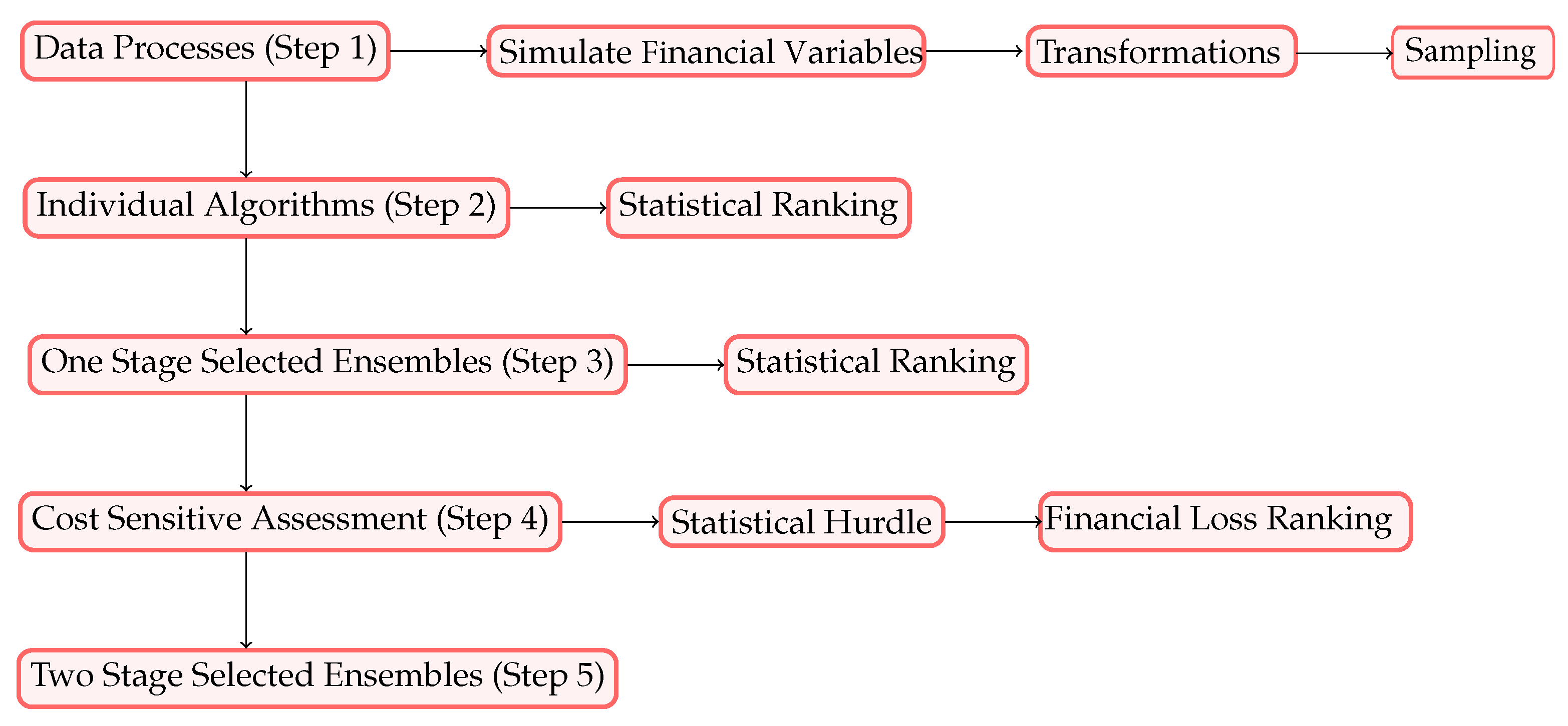
First, we describe the steps taken in our numerical experiments. Then, we illustrate the steps in Figure 1.

Step 1. 

(Data Processing): Starting with the GCD, randomly simulated financial variables were appended including loan term and principal amount, monthly repayments and balance owing, assuming an interest rate of $\%5.2$. At the portfolio level, the Loss Given Default (LGD) and Exposure at Default (EAD) were also calculated. The data were then transformed using the WoE, whereby all variables are made strictly increasing or decreasing. Lastly, the data were randomly sampled into train and test datasets.

Step 2. 

(Individual Algorithms): Taken from a variety of analytical approaches, 26 diverse classification algorithms were trained to predict credit risk and then ranked according to statistical metrics, including model accuracy and Gini.

Step 3. 

(Statistically Selected Stacking): Based on statistical performance in Step 2 and insights from prior research, which demonstrated differential performance on either side of the decision boundary, algorithms were combined into bespoke ensembles. The algorithms were trained to predict credit risk and then ranked according to statistical metrics (stacks ranged in size from two to as many as five algorithms).

Step 4. 

(Cost-Sensitive Selected Stacking): Stacks were created based on a two-step selection process. First, we utilized insights from the statistical metrics, which formed a minimum performance hurdle for further consideration. Second, the costs associated with false predictions were used to identify algorithms that resulted in the minimum cost for both dimensions of cost, i.e., default and opportunity costs. The stacks were identified by combining the algorithms that demonstrated the lowest default cost with those that presented the lowest opportunity cost in the two algorithm stacks.

Step 5. 

(Selected Stacking in Two Stages): We ranked all predictive approaches (with a minimum accuracy of at least >0.80) including individual algorithms, statistically selected stacks and stacks using both statistical and cost-sensitive considerations. We selected two algorithm ensembles by combining from a list of the lowest default and the lowest opportunity costs. The final performance comparison was obtained by ranking the lowest total cost, and the best-performing predictor or predictive combination was identified.

4. Empirical Results

Table 1. Full name and abbreviation for algorithms.

Full Name of Algorithms	Abbreviations
Additive Logistic Regression	ADA
AdaBoost	ADAB
Boosted Multi-Adaptive Regression Spline	BMARS
Conditional Random Forest	CRF
Decision Tree	C50
Deep Neural Network	DNN
Distance-Weighted Discrimination Polynomial	DWDp
eXtreme Gradient Boosting Linear	XGBl
eXtreme Gradient Boosting Tree	XGBt
Generalized Additive Model	GAM
Generalized Linear Model Network	GLMn
Gradient Boosting Machine	GBM
K-Nearest Neighbors	KNN
Linear Discriminant Analysis	LDA
Logistic Regression	LR
Multi-Adaptive Regression Spline	MARS
Multilayer Perceptron	MLP
Multilayer Perceptron Machine Learning	MLPm
Multi-Step Adaptive Elastic-Net	MSAe
Naive Bayes	NB
Neural Network	NNET
Partial Least Squares	PLS
Quadratic Discriminant Analysis	QDA
Random Forest	RF
Recursive Partitioning Decision Trees	RPAR
Support Vector Machine with Radial	SVMr

provides the abbreviations of the 26 individual algorithms used in this paper. All the algorithms are implemented in R using the functions/packages available. The parameters of the algorithms are the recommended values in the respected references.

Table 2. Error correlation matrix for 26 algorithms.

Models	ADA	ADAB	BMARS	C50	CRF	DNN	DWDp	GAM	GBM	GLMn	KNN	LDA	LR	MARS	MLP	MLPm	MSAe	NB	NNET	PLS	QDA	RF	RPAR	SVMr	XGBl	XGBt
ADA	1.00	0.98	−0.91	0.92	0.88	0.90	0.96	0.97	0.91	0.98	0.91	0.95	0.97	0.87	0.93	0.94	0.97	0.97	0.97	0.95	0.90	0.88	0.91	0.91	0.91	0.92
ADAB	0.98	1.00	−0.91	0.92	0.92	0.88	0.96	0.97	0.96	0.98	0.91	0.96	0.97	0.92	0.92	0.93	0.97	0.96	0.97	0.97	0.89	0.91	0.91	0.92	0.92	0.97
BMARS	−0.91	−0.91	1.00	−0.85	−0.78	−0.93	−0.89	−0.89	−0.85	−0.90	−0.86	−0.85	−0.89	−0.81	−0.87	−0.87	−0.89	−0.87	−0.88	−0.85	−0.83	−0.78	−0.90	−0.79	−0.84	−0.85
C50	0.92	0.92	−0.85	1.00	0.89	0.84	0.91	0.92	0.91	0.92	0.91	0.92	0.92	0.88	0.89	0.90	0.92	0.91	0.92	0.91	0.86	0.89	0.87	0.89	0.93	0.91
CRF	0.88	0.92	−0.78	0.89	1.00	0.75	0.90	0.91	0.97	0.91	0.88	0.94	0.91	0.95	0.87	0.88	0.90	0.91	0.91	0.93	0.83	0.98	0.85	0.94	0.90	0.96
DNN	0.90	0.88	−0.93	0.84	0.75	1.00	0.87	0.89	0.80	0.89	0.85	0.84	0.89	0.77	0.90	0.90	0.89	0.86	0.88	0.84	0.83	0.74	0.86	0.80	0.83	0.82
DWDp	0.96	0.96	−0.89	0.91	0.90	0.87	1.00	0.98	0.92	0.98	0.90	0.97	0.98	0.89	0.91	0.92	0.98	0.96	0.98	0.97	0.91	0.89	0.88	0.92	0.91	0.93
GAM	0.97	0.97	−0.89	0.92	0.91	0.89	0.98	1.00	0.94	1.00	0.91	0.99	1.00	0.90	0.94	0.95	0.99	0.97	0.99	0.97	0.90	0.90	0.88	0.95	0.92	0.94
GBM	0.91	0.96	−0.85	0.91	0.97	0.80	0.92	0.94	1.00	0.94	0.89	0.95	0.94	0.97	0.88	0.90	0.93	0.91	0.94	0.94	0.84	0.95	0.89	0.93	0.92	0.99
GLMn	0.98	0.98	−0.90	0.92	0.91	0.89	0.98	1.00	0.94	1.00	0.91	0.99	1.00	0.91	0.94	0.95	1.00	0.97	1.00	0.97	0.92	0.90	0.88	0.95	0.92	0.94
KNN	0.91	0.91	−0.86	0.91	0.88	0.85	0.90	0.91	0.89	0.91	1.00	0.89	0.90	0.85	0.89	0.89	0.90	0.90	0.90	0.91	0.86	0.87	0.92	0.86	0.89	0.91
LDA	0.95	0.96	−0.85	0.92	0.94	0.84	0.97	0.99	0.95	0.99	0.89	1.00	0.99	0.92	0.93	0.94	0.98	0.97	0.99	0.97	0.91	0.93	0.85	0.96	0.92	0.95
LR	0.97	0.97	−0.89	0.92	0.91	0.89	0.98	1.00	0.94	1.00	0.90	0.99	1.00	0.90	0.94	0.95	1.00	0.97	1.00	0.96	0.92	0.90	0.87	0.95	0.92	0.94
MARS	0.87	0.92	−0.81	0.88	0.95	0.77	0.89	0.90	0.97	0.91	0.85	0.92	0.90	1.00	0.85	0.86	0.90	0.87	0.90	0.91	0.81	0.93	0.84	0.91	0.89	0.96
MLP	0.93	0.92	−0.87	0.89	0.87	0.90	0.91	0.94	0.88	0.94	0.89	0.93	0.94	0.85	1.00	0.98	0.94	0.93	0.94	0.90	0.89	0.87	0.86	0.91	0.89	0.89
MLPm	0.94	0.93	−0.87	0.90	0.88	0.90	0.92	0.95	0.90	0.95	0.89	0.94	0.95	0.86	0.98	1.00	0.95	0.93	0.95	0.91	0.90	0.88	0.86	0.92	0.90	0.90
MSAe	0.97	0.97	−0.89	0.92	0.90	0.89	0.98	0.99	0.93	1.00	0.90	0.98	1.00	0.90	0.94	0.95	1.00	0.96	0.99	0.96	0.92	0.89	0.87	0.94	0.92	0.94
NB	0.97	0.96	−0.87	0.91	0.91	0.86	0.96	0.97	0.91	0.97	0.90	0.97	0.97	0.87	0.93	0.93	0.96	1.00	0.97	0.95	0.90	0.90	0.87	0.93	0.91	0.92
NNET	0.97	0.97	−0.88	0.92	0.91	0.88	0.98	0.99	0.94	1.00	0.90	0.99	1.00	0.90	0.94	0.95	0.99	0.97	1.00	0.96	0.92	0.91	0.87	0.95	0.92	0.94
PLS	0.95	0.97	−0.85	0.91	0.93	0.84	0.97	0.97	0.94	0.97	0.91	0.97	0.96	0.91	0.90	0.91	0.96	0.95	0.96	1.00	0.88	0.91	0.87	0.93	0.91	0.95
QDA	0.90	0.89	−0.83	0.86	0.83	0.83	0.91	0.90	0.84	0.92	0.86	0.91	0.92	0.81	0.89	0.90	0.92	0.90	0.92	0.88	1.00	0.82	0.81	0.87	0.86	0.85
RF	0.88	0.91	−0.78	0.89	0.98	0.74	0.89	0.90	0.95	0.90	0.87	0.93	0.90	0.93	0.87	0.88	0.89	0.90	0.91	0.91	0.82	1.00	0.83	0.94	0.91	0.94
RPAR	0.91	0.91	−0.90	0.87	0.85	0.86	0.88	0.88	0.89	0.88	0.92	0.85	0.87	0.84	0.86	0.86	0.87	0.87	0.87	0.87	0.81	0.83	1.00	0.81	0.85	0.90
SVMr	0.91	0.92	−0.79	0.89	0.94	0.80	0.92	0.95	0.93	0.95	0.86	0.96	0.95	0.91	0.91	0.92	0.94	0.93	0.95	0.93	0.87	0.94	0.81	1.00	0.90	0.93
XGBl	0.91	0.92	−0.84	0.93	0.90	0.83	0.91	0.92	0.92	0.92	0.89	0.92	0.92	0.89	0.89	0.90	0.92	0.91	0.92	0.91	0.86	0.91	0.85	0.90	1.00	0.93
XGBt	0.92	0.97	−0.85	0.91	0.96	0.82	0.93	0.94	0.99	0.94	0.91	0.95	0.94	0.96	0.89	0.90	0.94	0.92	0.94	0.95	0.85	0.94	0.90	0.93	0.93	1.00

presents a Pearson correlation matrix of the errors associated with each algorithm. In this table, algorithms with an error correlation of less than 0.1 are in bold. Broadly, the algorithms with errors that show the lowest average Pearson correlation with each of the others were RPAR, followed by RF and then the MLP. Ensembles were created based on individual performance in a single algorithm testing, the correlation between error terms from each algorithm (low correlation between errors is a common strategy to identify stacking combinations) and, lastly, use of prior research.

Table 3. Comparative statistical performance for individual algorithms (Step 2).

Model	Accuracy	Gini	AUC
GAM	0.8700	0.8812	0.9406
LR	0.8667	0.8769	0.9385
ADA	0.8667	0.8751	0.9376
MARS	0.8667	0.8681	0.9341
DWDp	0.8633	0.8902	0.9451
GLMn	0.8633	0.8825	0.9413
XGBt	0.8633	0.8785	0.9393
MSAe	0.8633	0.8727	0.9363
PLS	0.8633	0.8693	0.9347
KNN	0.860	0.8540	0.9270
ADAB	0.8567	0.8796	0.9398
C50	0.8567	0.8543	0.9271
GBM	0.8533	0.8817	0.9408
NNET	0.8533	0.8810	0.9405
XGBl	0.8467	0.8423	0.9212
LDA	0.8433	0.8709	0.9354
MLPm	0.8433	0.8607	0.9304
NB	0.8433	0.8526	0.9263
RF	0.8400	0.8661	0.9331
MLP	0.8367	0.8566	0.9283
SVMr	0.8333	0.8403	0.9202
QDA	0.8300	0.8074	0.9037
RPAR	0.8267	0.8121	0.9061
CRF	0.8100	0.8779	0.9389
DNN	0.7000	0.8131	0.9066
BMARS	0.1367	0.8372	0.9186

summarizes statistical metrics (accuracy, Gini and AUC) of the individual algorithms and ranks them according to their respective accuracy. The results from this table show that while all individual algorithms passed the 0.80 hurdle for Gini, neither the DNN nor BMARS passed the 0.80 accuracy hurdle and, subsequently, were excluded from consideration for ensembles. A further insight into the performance of the DNN indicates that it predicted all test observations as negatives (non-defaulters), while, for BMARS, the reverse was true, predicting an elevated number of positives (defaulters). It is noteworthy that this was picked up only by model accuracy, with neither model’s Gini nor AUC is within a normal range. This suggests some utility in using multiple performance metrics yet underscores the issues with applying linearly related assessment approaches. Further, comparing the performance of the other 24 algorithms shows a very narrow difference between their performances, which achieved the minimal benchmark of 0.80, ranging from 0.81 to 0.87. While the GAM had the highest accuracy, it was only marginally better than LR. Given the simpler formulation, it is likely that LR would be selected under these circumstances.

In

Table 4. Comparative accuracy performance for best statistically selected stacking ensembles (Step 3).

Ensemble	Accuracy	Gini	AUC
ADA, QDA, C50	0.8767	0.8811	0.9405
MARS, BMARS	0.8767	0.8800	0.9400
PLS, LDA, XGBt, NNET, NB, DWDp	0.8700	0.8897	0.9449
GLM, KNN	0.8700	0.8779	0.9389
CRF, MLPm, MSAe, GLMn	0.8667	0.8913	0.9457
SVMr, XGBl	0.8667	0.8734	0.9367
GLM, RPAR, GBM, MLP, RF	0.8633	0.8835	0.9417
MLP, RF	0.8633	0.8764	0.9382
GLM, RPAR, GBM, MLP, RF, SVMr	0.8633	0.8879	0.9440
RF, GLM, RPAR, GBM	0.8633	0.8869	0.9434

, we provide the statistical performance for the top 10 stacking combinations. Here, the algorithms were selected for inclusion into bespoke ensembles based on the statistical performance demonstrated in previous steps and in prior research. The top two ensembles selected using statistical metrics had better accuracies than the best individual algorithm, the GAM.

Seeking to improve the quality of credit risk assessment, the next phase of bespoke ensembles comprises a two-stage selection process. Firstly, they must exceed a minimum accuracy benchmark of 0.80. All individual algorithms that met this standard were available for selection in the next stage, which assesses performance according to the financial performance metric. The second process involves using the financial performance metric to calculate opportunity and default cost for each of the 24 algorithms and then selecting the best-performing algorithms according to those that resulted in the lowest value for these two cost dimensions. This was achieved by selecting the 10 lowest default cost algorithms and combining these with the 10 lowest opportunity cost algorithms to create bespoke two-algorithm ensembles.

Table 5. Individual algorithms sorted by lowest default cost (USD millions) (Step 4).

Algorithm	Default Cost	Opportunity Cost	Total Cost	Accuracy
PLS	148	362	510	0.8633
KNN	168	342	510	0.8600
XGBt	172	343	515	0.8633
ADA	174	350	523	0.8667
MARS	188	356	544	0.8667
DWDp	191	304	495	0.8633
NNET	192	397	588	0.8533
C5.0	192	294	487	0.8567
LDA	198	432	630	0.8433
ADAB	198	356	553	0.8567

and

Table 6. Individual algorithms sorted by lowest opportunity cost (USD millions) (Step 4).

Algorithm	Opportunity Cost	Default Cost	Total Cost	Accuracy
CRF	99	580	679	0.8100
RF	261	287	548	0.8400
DTr	286	323	608	0.8267
GAM	287	200	487	0.8700
LR	286	218	504	0.8667
C5.0	294	192	487	0.8567
NB	297	301	598	0.8433
DWDp	304	191	495	0.8633
XGBl	308	210	518	0.8467
GLMn	317	209	526	0.8633

report algorithm performance based on financial performance. While Table 5 shows the lowest 10 ranked by default cost, Table 6 shows the same information now ranked by lowest opportunity cost.

Combining the algorithms according to the lowest default and opportunity costs enabled us to develop low-cost ensembles optimally; these are denoted with the suffix ‘F’ and are tabulated below (

Table 7. Comparison of financial (USD millions) and statistical performance for final stage stacking (Step 5). ‘F’ denotes ensembles created using financial loss information.

Model	Opportunity Cost	Default Cost	Total Cost	Accuracy	Gini	AUC
RF, KNN (F)	230	187	417	0.8533	0.8723	0.9362
GAM, MARS (F)	224	202	425	0.8700	0.8828	0.9414
CRF, MARS (F)	223	203	426	0.8600	0.8756	0.9378
GAM, ADA (F)	224	203	427	0.8533	0.8799	0.9399
CRF, PLS (F)	234	190	424	0.8600	0.8803	0.9402
RF, PLS (F)	255	208	463	0.8533	0.8762	0.9381
CRF, MLPm, MSAe, GLMn	303	177	480	0.8667	0.8913	0.9457
ADA, QDA, C50	357	123	480	0.8767	0.8811	0.9405
PLS, LDA, XGBt, NNET, NB, DWDp	293	188	481	0.8700	0.8897	0.9449
SVMr, XGBl	258	224	481	0.8667	0.8734	0.9367
LR, RPAR, GBM, MLP, RF	310	173	483	0.8633	0.8835	0.9418
RF, XGBl	304	182	485	0.8567	0.8621	0.9311
LR, KNN	270	215	485	0.8700	0.8779	0.9389
RF, LR	315	173	488	0.8600	0.8790	0.9395
GAM	287	200	487	0.8700	0.8812	0.9406

). This table ranks performance by lowest misclassification cost. It is noteworthy that the ensembles developed using financial criteria present the lowest misclassification cost, followed by the best statistically developed ensembles. For comparison, the best individual algorithm, the GAM, is also shown.

Table 7 demonstrates that there is only a very minor difference in statistical performance, ranging in accuracy from 0.8533 to 0.8767. Ranked by the total cost, it is clear that the ensembles resulting in the lowest losses are those selected based on combining the lowest default costs with those showing the lowest opportunity cost. The difference in cost between the best individual algorithm and the best financial performance selected ensemble is to the order of USD 70 million, a commercially significant difference, especially if this small sample was scaled up to the size and value of portfolios observed in large retail banks.

5. Discussion and Conclusions

The primary goal of every financial institution is to make a profit for shareholders, which is broadly achieved by optimally identifying, estimating and managing risks. Traditionally, models are selected based on a very narrow range of assessment metrics, which are dominated by statistical performance. However, we propose that an additional lens seeking to evaluate the comparative costs associated with model selection will significantly improve credit risk outcomes for lenders and any binary decision process with asymmetrical outcomes.

In this paper, we showed that heterogeneous ensembles selected based on statistical performance according to commonly used metrics, such as model accuracy and Somers D (Gini), provided some uplift compared to individual algorithms. We then showed that by adding a second model ranking stage to model selection based on the lowest financial costs attributable to both positive and negative false predictions, performance was enhanced even further. As benchmark statistical performance was already established, model selection with the additional financial criteria reduced the cost of losses due to misclassifications and therefore improved the quality of credit risk decisions.

Incorporating financial costs as a second dimension of algorithm selection further enhanced predictive capabilities, which aligns with the commercial objectives of the credit provision for financial organizations. By first setting a statistical performance hurdle and then selecting algorithm stacks that combine the lowest default and opportunity costs, the overall costs due to losses were minimized. In other words, misclassification costs were minimized by selecting and combining algorithms that achieved the lowest cost on either side of the binary outcome, i.e., both false positives (opportunity cost) and false negatives (default cost).

Estimating the costs of misclassifications in this way is a novel approach that expands on the philosophy of cost-sensitive learning as described by Elkan [50]. We incorporate advances in understanding the losses derived from research into loss accounting, such as investigations that have led to the development of the IFRS9 standard. In addition, setting statistical metrics as a benchmark and then using financial metrics to rank models has enabled this study to identify the models that provide adequate statistical performance and result in the lowest misclassification costs. When these findings on a small dataset of 1000 applicants are expanded to the scale seen in retail lending, we estimate a financial benefit of hundreds of millions of dollars per year.

The combination of the proposed financial criteria and statistical metrics can be deployed in any environment to improve their decision-making on commercial applications. Credit risk is a good example of this, where misclassifications will rarely result in the same overall cost due to varying magnitudes of the underlying principal loan amount, loan tenor and interest rates.

In applications such as the credit risk scenario used here, there can be a reticence to pursue more complex predictive methods than Logistic Regression, due to perceived issues such as a lack of transparency and explainability or difficulties with prudential supervisory approval for Internal Ratings -Based (IRB) models. However, in a survey of prudential standards in jurisdictions such as Australia, the UK, the EU, Canada and the USA, there are no formal restrictions to the types of models allowed, particularly regarding credit scorecards, which have little impact on regulatory capital.

In this paper, the optimal predictive approach identified combines Random Forest, which comprises a homogeneous ensemble of a series of decision trees, stacked together with K-Nearest Neighbors. In terms of individual algorithms, the Generalized Additive Model performed best overall, providing enhanced statistical and loss performance at the cost of only a minor uplift in complexity that comes with optimizing the number of splines and thus specifying knots and so-called wiggliness. Therefore, in single-algorithm models, the Generalized Additive Model may provide an excellent alternative to Logistic Regression, particularly in portfolios where non-linearity is observed, such as where brands with different underwriting standards have been combined under one model.

As is commonly observed, replicating these results on more diverse, larger datasets may serve to strengthen our findings and uncover new relationships. Future research should expand this work by seeking to evaluate whether the same algorithms selected under the same approach used here for credit scorecards is an effective strategy for use on the behavioral probability of default models, which have the largest impact on regulatory capital and receive therefore much greater scrutiny by prudential bodies. In addition, simulation-based studies may serve to further underscore the value of the financial performance metric across different types of risks with different magnitudes.