Abstract
The growing emphasis on ecological preservation and natural resource conservation has significantly advanced resource recycling, facilitating the realization of a sustainable green economy. Essential to resource recycling is the pivotal stage of disassembly, wherein the efficacy of disassembly tools plays a critical role. This work investigates the impact of disassembly tools on disassembly duration and formulates a mathematical model aimed at minimizing workstation cycle time. To solve this model, we employ an optimized advantage actor-critic algorithm within reinforcement learning. Furthermore, it utilizes the CPLEX solver to validate the model’s accuracy. The experimental results obtained from CPLEX not only confirm the algorithm’s viability but also enable a comparative analysis against both the original advantage actor-critic algorithm and the actor-critic algorithm. This comparative work verifies the superiority of the proposed algorithm.
Keywords:
disassembly line balancing; tool deterioration; reinforcement learning; advantage actor-critic algorithm MSC:
90-08
1. Introduction
The ongoing acceleration of scientific and technological advancements has led to a continual proliferation of electronic technology products. This rapid evolution in electronic information technology has profoundly reshaped our lifestyles, markedly enhancing our quality of life. However, alongside the benefits derived from these technologies, they have produced significant challenges, including the depletion of global resources and the progressive degradation of the Earth’s ecology. The accelerated pace of updates in electronic products has amplified electronic waste generation. In 2021 alone, global electronic waste surpassed 57 million tons, signifying an immense squandering of resources and posing a substantial threat to humanity. Addressing these issues has brought the recycling and remanufacturing of waste products into sharp focus [1,2,3]. According to relevant agency data, recycling End-of-Life (EOL) products within the iron and steel domain can curtail mining waste by 97%, air pollution by 86%, water pollution by 76%, water consumption by 40%, raw materials by 90%, and energy by 74%. These figures robustly underscore the pivotal role of recycling and remanufacturing [4,5]. As illustrated in Figure 1, the remanufacturing process chiefly encompasses recycling, disassembly, detection, classification, remanufacturing, and other sequential steps. The concept of EOL product disassembly was first introduced by Gupta in 1994 [6,7,8]. Disassembly facilitates the retrieval of intact product parts, ensuring their continued utility, optimizing resource utilization, and mitigating the adverse impacts of EOL products on human health and the environment. Notably, disassembly emerges as the intricate primary stage in remanufacturing, directly influencing recycling efficiency and remanufacturing costs.
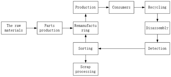
Figure 1.
The remanufacturing process.
A comprehensive disassembly process involves determining the disassembly sequence and arranging disassembly workstations, as shown in Figure 2. Uneven workstation distribution during disassembly impacts efficiency and increases costs. Consequently, scholars have proposed the Disassembly Line Balancing problem (DLBP). Gao et al. [9] extensively investigated setting the number of active workstations and idle rates in dismantled lines to meet environmental resource requirements while ensuring targeted dismantling efficiency. The meticulous design of a disassembly line, balancing diverse factors influencing the process, holds profound significance for advancing the recycling and remanufacturing industry. Numerous studies [10,11,12,13,14,15] delve into various disassembly lines and their classifications. For example, according to the layout of disassembly lines, they can be divided into parallel disassembly lines, bilateral disassembly lines, U-shaped disassembly lines, and linear disassembly lines. The type of disassembly can be divided into complete disassembly and selective disassembly. Some studies [16,17,18,19] meticulously examine these methods, noting that selective disassembly adheres to objective function constraints, whereas complete disassembly involves dismantling all parts, making it suitable for less damaged or highly profitable products. General electronic equipment often gets discarded due to irreparable damage. Since complete disassembly entails dismantling all product parts, the disassembly sequence becomes pivotal—the forefront of product disassembly. Maximizing the disassembly value relies on a well-crafted disassembly sequence, enhancing workstation configuration efficiency and overall disassembly effectiveness. Early observations by Seliger et al. [20] highlighted the effect of disassembly tools in improving efficiency and reducing removal risks. However, the inevitable tool wear during disassembly affects the usage time and costs significantly. Therefore, accounting for tool wear is pivotal in addressing DLBP.

Figure 2.
Straight disassembly layout.
Currently, the primary approaches for tackling the disassembly line balance problem encompass exact algorithms, heuristic algorithms [21], and meta-heuristic algorithms. Theoretically, exact algorithms aim to resolve the disassembly line balance precisely. Yet, due to the NP complexity of the DLBP, they can only handle small-scale problems, proving inadequate for larger-scale ones. While heuristic algorithms are simple, they often lack high solution accuracy, limiting their efficacy for large-scale disassembly problems, albeit contributing to hastening the convergence of meta-heuristic algorithms. Meta-heuristic algorithms, proficient in efficiently solving large-scale DLBP instances, offer satisfactory solutions within short time frames. Despite the accuracy and advantages of exact algorithms in resolving small-scale problems, their limitations hinder their applicability to larger-scale ones. Consequently, meta-heuristic algorithms, including genetic algorithms, neighborhood search algorithms, artificial fish swarm algorithms, cat swarm algorithms, firefly algorithms, and artificial bee colony algorithms, shoulder the task of handling large-scale disassembly challenges. Extensive research validates the prowess of intelligent optimization algorithms in swiftly addressing large-scale problems, resulting in their widespread adoption in addressing the disassembly line balance problem.
Machine learning involves various fields, and neural networks attract increasing favor. For instance, some studies [22,23,24,25] use networks for gesture recognition. Reinforcement learning issues play a pivotal role in solving optimization problems and scheduling. It solves large-scale problems swiftly. Researchers conduct various studies on reinforcement learning, expanding its use scenarios. Ji et al. [26] and Zhou et al. [27] researched scheduling. S. Mete et al. [28] made the first attempt to apply reinforcement learning in disassembly line balancing. E. Tuccel et al. [29] used reinforcement learning algorithms for large-scale disassembly line balancing and verified its faster solving speed compared with conventional methods. Additionally, M. Everett and S. Woo [30,31] conducted research on dynamic actions and decision-making. This paper adopts a new technique by using reinforcement learning instead of meta-heuristic algorithms to solve DLBP. It employs a flexible AND/OR graph model that easily maps to reinforcement learning, and neural networks in the algorithm accelerate the agent’s learning process.
In summary, this work employs reinforcement learning algorithms to address the comprehensive disassembly-based disassembly line balance problem (DLBP), enabling continuous learning for the agent until it achieves a satisfactory solution. Contrasted with the prevailing conventional methods, the primary contributions of this research encompass the following aspects:
- 1.
- We examine the single-objective, single-column disassembly line balance issue to minimize workstation cycle time, considering the influence of disassembly tool degradation on the disassembly duration.
- 2.
- We employ the A2C reinforcement learning algorithm to address the DLBP. In our DLBP representation, the disassembly task and workstation are considered to be actions, allowing for the simultaneous selection of the disassembly task and the workstation. To streamline the algorithm’s functionality, we have implemented measures to prevent illegal actions, thereby reducing the action space and enhancing algorithm convergence speed. Additionally, we have integrated the greedy strategy into the algorithm for further expedition of convergence.
- 3.
- This research conducts comparative tests across six cases. It compares the outcomes of A2C algorithms implemented with and without the integration of the greedy strategy and dynamic action space. The results demonstrate the efficacy of the greedy strategy. Furthermore, the enhanced A2C algorithm exhibits superior performance compared with the AC algorithm results.
The paper has five main parts. The second segment outlines the addressed disassembly line balancing problem, while the third segment explicates the A2C algorithm. The fourth part primarily details the experimental design and the comparative analysis of the experimental results. Lastly, the fifth section encapsulates a comprehensive summary of the entire paper.
2. Problem Description
2.1. Problem Statement
The DLBP is considered when assigning disassembly tasks to workstations under various constraints. This paper studies the complete disassembly of linear disassembly lines. The disassembly task is assigned to the workstation under a certain workstation cycle time, and the impact of the degradation rate of the disassembly tool on the disassembly time is considered, and the workstation cycle time is minimized [32,33,34,35]. A complete disassembly line includes a disassembly workstation, a disassembly location, a disassembly task, and disassembly tools. The disassembly tool considered in this paper is a vulnerable tool. When the tool does the same thing again, the disassembly time will be longer. We assume that different disassembly tools disassemble different parts during the product disassembly process and use the tool’s degradation coefficient to represent the impact on disassembly time. Through the continuous use of tools during the dismantling process, the dismantling time has been improved, and the losses suffered by dismantling tools vary depending on the dismantling task.
The total disassembly time of a workstation is influenced by the degree of degradation in the disassembly tool due to the fixed original disassembly time for each component. As illustrated in Figure 3, tool 1 in workstation 1 is capable of disassembling both tasks 1 and 5. However, after completing task 1, tool 1 undergoes deterioration. Consequently, the dismantling time of task 5 will be affected if tool 1 is used for dismantling. Therefore, when considering the allocation of workstations, we also need to consider the degradation of dismantling tools to minimize the dismantling time cost of our workstations.
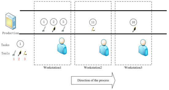
Figure 3.
Disassembly scheme considering tool.
An AND/OR graph depicts the disassembly process, incorporating information on disassembly tasks, disassembly subassemblies, and disassembly parts. The AND/OR diagram not only signifies the prioritization of disassembly tasks but also indicates the dependency relationships among subassemblies and parts. It comprises rectangles and directed angles, where a rectangle represents the subassembly number and part information. More precisely, the numbers within the angle brackets represent the subassembly number, while the letters outside the angle brackets represent the part information within the subassembly. Each directional angle corresponds to a decomposition task, with the number within the angle denoting the task number and the arrow symbolizing the relationship between subassemblies. The arrow tail points to the detachable subassembly, whereas the arrow points to the subassembly obtainable after disassembling the current subassembly. There are many directional angles before and after the rectangle, but the same subassembly can only perform one disassembly task; that is, it can only perform one directional angle. Utilizing the AND/OR graph, we can transform the disassembly problem into a graph-solving procedure, subsequently introducing various constraints to obtain optimal solutions. In the context of employing reinforcement learning for DLBP problems, the AND/OR graph can be viewed as an environment for agent interaction. To effectively combine disassembly line problems, we convert the task precedence relationship and conflicting task relationship represented in the AND/OR graph into matrix form, upon which algorithms can be applied.
Figure 4 illustrates the composition of the kettle, while Figure 5 represents the disassembly AND/OR graph for the basic kettle subassembly. The AND/OR graph entails various constraints that include conflicted relationships, task priorities, and task-subassembly relationships. As demonstrated in Figure 5, the disassembly process involves 19 subassemblies, 8 parts, and 14 disassembly tasks. The conflict and priority relationship of tasks needs to be met in the disassembly process. For instance, subassembly 1 can disassemble subassembly 2 and subassembly 10 through task 1, and subassembly 2 can subsequently proceed with downward disassembly tasks. Specifically, subassembly 2 can undertake disassembly tasks 3 and 4. However, a conflict arises when attempting to perform these two tasks simultaneously, allowing only one task to be executed. Consequently, disassembly task 1 cannot be repeated.
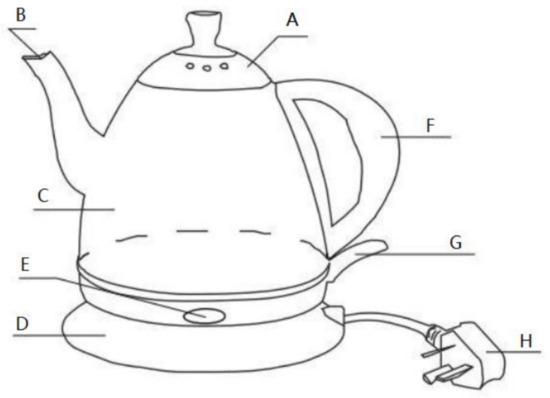
Figure 4.
Structure of the hot water kettle.
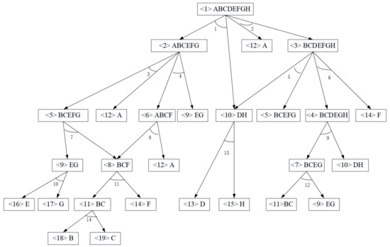
Figure 5.
An AND/OR graph of the kettle.
The conflicted relationship, precedence relationship of tasks, and correlation between tasks and subassemblies are discernible from the AND/OR graph. For the algorithm to effectively utilize these relationships, we employ matrix representation to express them. The following describes these relationships.
(1) To describe the conflicted relationship of each task, we added the conflict matrix , where
(2) To describe the relationships between individual tasks and components, we built the task-component relationship matrix , where
(3) To describe the relationships between individual tasks and tools, we built the task-tool relationship matrix , where
According to the provided formula, the conflict matrix C of the kettle can be defined as follows. From Figure 5, we can see that task 1 is executed before task 3, so is set to 1. Furthermore, since task 1 and task 2 both disassemble the same subassembly and cannot be performed simultaneously, values of -1 are assigned to and , with 0 being assigned in other cases.
Similarly, the relationship matrix B for the kettle can be defined as follows. As can be seen from Figure 5, component 9 can be disassembled by task 10 to obtain parts 16 and 17 from it, so and are set to 1. It is set to 0 for other task-component combinations for which parts cannot be obtained. For example, component 6 can be disassembled by task 8, from which part 12 and component 8 are obtained. Therefore, is set to 1, while is set to 0.
The following is the definition of the relationship between individual tasks and tools in matrix D for the kettle. Based on the complexity of the DLBP and the DLBP addressed in this work, we make the following assumptions for the mathematical model.
- 1.
- We adopt linear single-target disassembly.
- 2.
- One subassembly can only be removed by one disassembly tool.
- 3.
- All disassembled parts are to be removed.
- 4.
- The degradation rate of disassembly tools has been determined.
- 5.
- The disassembly time of tools used on each workstation for each task is known.
- 6.
- Workstations are started in sequence.
- 7.
- Each task is disassembled only once during the disassembly process.
2.2. Notations
I Number of tasks.
W Number of workstations.
N Number of subassemblies.
R Number of tools.
K Number of task locations.
Collection of workstations .
Mission collection .
Collection of components .
Collection of task locations on the workstation .
Collection of tools .
Matrix of tasks j that conflict with task i.
Precedence task j matrix for task i.
w Workstation index, .
n Subassembly index, .
Task indexes, i, .
k Location index, .
Normal disassembly time of task i on workstation w.
Deterioration coefficient of processing task i on the workstation w.
An element in the n-th row and i-th column of B.
An element in the i-th row and r-th column of D.
Decision variables:
(1)
(2)
(3) The time that tool r on the w-th workstation has been used before task i is executed.
(4) Actual disassembly time of task i on the w-th workstation, which is the dismantling time considering the impact of tool deterioration.
(5) Maximum working time of a workstation.
2.3. Mathematical Model
The objective function (14) of this study aims to minimize the maximum working time of workstations. Constraint (2) ensures that each task is executed at most once. Constraint (3) guarantees that workstations are activated sequentially. Constraint (4) restricts each location on a workstation to execute only one task. Constraint (5) ensures that if there is a task in the last position of a workstation, there must be a task in the previous position as well. Constraint (6) allows for the execution of only one conflicting task at most. Constraint (7) imposes a limitation on the number of open workstations. Constraint (8) mandates that an open workstation must be assigned tasks. Constraint (9) determines whether a workstation is enabled. M represents an infinite number. Constraint (10) ensures that the disassembly task sequence adheres to the task priority relation. Constraint (11) calculates the usage time of disassembly tool r on workstation w prior to the execution of task i. Constraint (12) calculates the actual disassembly time of task i using disassembly tool r on workstation w. Lastly, constraint (13) guarantees the disassembly of all parts.
3. Proposed Algorithm
3.1. Advantage Actor-Critic Algorithm Description
This section introduces the A2C algorithm in reinforcement learning. The A2C algorithm is an optimization algorithm based on the actor-critic (AC) [36] algorithm, which has become relatively mature in the current stage of reinforcement learning. Unlike algorithms that make decisions based on values, the A2C algorithm is based on policy calculation. In terms of algorithm structure, the A2C algorithm not only combines two neural networks but also utilizes an advantage function to evaluate the quality of actions, enabling the agent to learn better. When evaluating the quality of actions, the A2C algorithm uses the advantage value calculated by the advantage function as the evaluation criterion, reducing the variability of action selection and making the learning of the agent more stable. Like the AC algorithm, the A2C algorithm establishes two neural networks, using the actor and critic networks to select and evaluate the agent’s behavior. Compared with the AC algorithm, the A2C algorithm adds an advantage function to stabilize the policy. The original A2C algorithm (o-A2C) algorithm cannot reduce action space compared with the A2C algorithm. The size of the action space of the o-A2C algorithm will sharply increase in solving large-scale problems, thus increasing the time and space complexity of the algorithm, which is costly for us.
The implementation of the algorithm mainly involves the actor continuously selecting actions based on the environment. Then, based on feedback from the environment (value from the critic), the next action to choose is determined. Participants choose the following action based on its probability, computed using the critic’s return value. Once the actor completes an action, it returns the new state and value to the critic. The critic then calculates the TD error value of the return value, which is subsequently used to update the action probability for the actor. This process repeats until the termination condition is satisfied. Figure 6 displays the algorithm architecture of A2C.
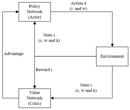
Figure 6.
The algorithm architecture of A2C.
3.2. Algorithm Mechanism of A2C
In the A2C algorithm, the actor-network generates action policies to control the behavior of the agent. The critic network evaluates these behaviors through value functions and updates the policies by comparing the quality of actions. It uses an advantage function to measure the advantage of taking a certain action relative to the average level. This approach enables more precise guidance for policy updates.
This article designs action, state, and reward based on the characteristics of DLBP. The action a in the algorithm includes selected disassembly tasks and workstations. The state s includes the components, workstations, and location information at a certain moment during the disassembly process. The reward r of the algorithm is the disassembly time in the current state. The following are some formulas of the A2C algorithm:
We represent the value of action a in a given state s as . This paper focuses on the execution of disassembly task i on workstation w when in state s, and measures the reward of the current action based on the obtained results. The reward is set as the cycle time of the workstation during the execution of the disassembly task. represents the value of the subsequent state.
Equation (16) represents the advantage function in the A2C algorithm, demonstrating the linear relationship between Q and V. This equation quantifies the advantages of an action compared with the average value in state s, promoting a balanced advantage value across the entire strategy. If the advantage value is less than 0, it indicates that this action is inferior to the average and not a good choice.
Formula (17) represents the gradient of the actor-network parameter update, where is the objective function of the actor-network, and is the probability of action output by the policy network in state s. is an advantage function that represents the advantage of an action relative to the average action taken under state s. in the formula represents the expected value when selecting an action according to the policy . We update the actor-network parameters through Formula (17).
We insert Formula (15) into Formula (17) and obtain an optimized Formula (18). All decision values are calculated in a neural network, making the results more stable.
According to Figure 6, we can get the algorithm structure figure. The environment interacts with the two networks and constantly updates actions through action a, reward r, and the advantage value of the actions. From this, we can obtain the pseudocode of the algorithm as shown in Algorithm 1. Among them, refers to the decay factor used to calculate the discount of the reward in the TD error, which is set to 0.7 in this paper. is the learning rate, which we set to 0.001 for the actor and 0.01 for the critic. Advantage A is given in Equation (16).
| Algorithm 1 Advantage Actor-Critic (A2C). |
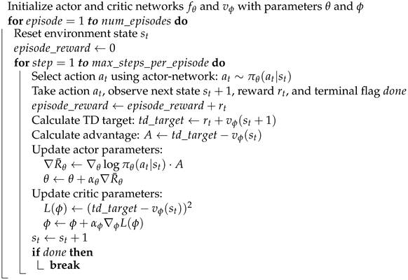 |
3.3. Action and State of DLBP
The A2C algorithm in DLBP requires redefining actions due to the presence of a single agent. To enable the agent to handle both the disassembly task sequence and workstation allocation problems simultaneously, we represent actions as combinations. In the process of solving DLBP, two problems need to be addressed: determining the sequence of disassembly tasks and allocating workstations. Thus, we define the operation as a combination of task (i) selection and workstation (w) selection. In our case study on a water kettle, Figure 5 comprises 14 disassembly tasks. We assume that three workstations are open. The size of the operating space can be set as the product of the number of disassembly tasks and the number of open workstations. For example, the selection of action 1 corresponds to executing disassembly task 2 at workstation 1, while selecting action 15 corresponds to the execution of disassembly task 2 at workstation 2.
Figure 6 illustrates the status of disassembly using the following variables: w for the disassembly workstation, c for the disassembly subassembly, and k for the disassembly workstation location. Following Figure 5, we utilize a kettle as a case study and perform the disassembly process of breaking down subassembly 1 in order to acquire sub subassembly 2 and subassembly 10. The initial phase of disassembly is characterized by specific sequence constraints, including the requirement for task 1 to be taken apart at the first position of workstation 1. Subsequently, subcomponents 2 and 10 may be disassembled at either workstation 1 or workstation 2, thus representing the initial disassembly state as the first position of subcomponent 1 disassembly on workstation 1.
3.4. The Definition of Environment
The precedence relationship matrix and association matrix B obtained from the AND/OR graph are incorporated as constraint conditions in the algorithm environment. Disassembly tasks, subassemblies, workstations, and workstation positions serve as component elements within this environment. The initial setup of the environment is with the disassembly workstation, including its location, disassembly tasks, and subassemblies, which are all set to zero to initiate the disassembly process. This indicates that subassembly 1 is dismantled by task 1 at the first position of workstation 1. Considering the constraints of the DLBP model, which mandates the complete disassembly of all subassemblies, a variable is introduced within the algorithm environment to serve as an identifier for the disassembled parts. Each disassembled part is assigned an identifier to mark the completion of the algorithm.
The Step function of the A2C facilitates the disassembly of subassemblies using logic based on complete disassembly. Initially, the subassemblies obtained from the state are decomposed and stored in an array, considering the relationships between tasks and subassemblies. A matrix representing the relationships between subassemblies and parts is then employed to determine whether the subassemblies in the array consist of individual parts, thus indicating the achievement of complete disassembly. Figure 7 illustrates the subassemblies and parts matrix (). If a retrieved component contains only one part, a single part identifier is adjoined, and the search proceeds to the next element in the pattern. Otherwise, to complete the subsequent step, the search is terminated. The time required for disassembling subassemblies is determined by multiplying the tool degradation rate by the time the tool has been in use and then multiplying that result by the initial time. By calculating the dismantling time for each disassembly task, we obtain the total dismantling time for the corresponding workstation, stored in a one-dimensional array labeled with the workstation number. Finally, the maximum disassembly time of the workstation is computed.
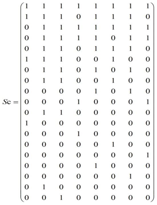
Figure 7.
Graph of the subassembly and part relationships.
3.5. The Specific Reduction of Action Space
We optimize the action space using Algorithm 2 to enhance its descriptive capabilities. The method starts by acquiring probabilities for all actions from the neural network. Then, it filters out illegal actions based on the current state and constraints of the problem. Afterward, it standardizes the probabilities of the remaining actions. Finally, a valid action is randomly selected from it as the action for this step.
| Algorithm 2 Choose Action. |
| Input: Parameters of the actor-network: θ, state: s |
| Output: Action a |
| 1: Obtaining action probability distribution πθ(a|s) via actor-network. |
| 2: The illegal actions are removed from the action space. |
| 3: Standardizing Action-space Probability Distributions. |
| 4: An action chosen at random from the action space: a |
| 5: return a |
In our scenario, assuming there are three open workstations, there are 13 disassembly tasks in total. As stated in the previous section, we represent actions as combinations of disassembly tasks and workstations, resulting in an action space size of 42 (the total number of actions). We assign the number 0 as the initial action in the action space. Thus, actions 0–13 correspond to 13 tasks removed from the first workstation, actions 14–27 represent 13 tasks removed from the second workstation, and so on. Via the relationship matrix, task 1 serves as the predecessor of tasks 3 and 4. Subsequently, after the completion of task 1, the action space is updated to include the sole operations for selecting tasks 3 and 4, as they can exclusively be performed on workstations 1 and 2. Consequently, we populate the new action space with the corresponding actions. Specifically, the actions numbered 2, 3, 16, and 17 are selected from the initial action space to form the new action space, reducing its size from 42 to 4. The process of the action space reduction after selecting action 1 is illustrated in Figure 8.
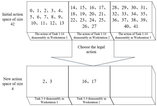
Figure 8.
The optimization process of action space.
To sum up, the following strategies are mainly used in the combination of the A2C of reinforcement learning and DLBP.
- 1.
- The action in the joint learning selection of the disassembly sequence and workstation assignment is determined based on the correlation between the disassembly task and the disassembly workstation.
- 2.
- We represent the relationship between subassemblies and parts in the form of a matrix to achieve the complete disassembly of the product.
- 3.
- We dynamically adjust the action space to accommodate the various disassembly objects in DLBP. This adjustment helps in reducing the selection of invalid actions and the associated time complexity.
4. Case Study and Result Analysis
We utilize the A2C algorithm and CPLEX solver to solve the model separately. We compared the running times of both algorithms and assessed the optimal solution to validate the model’s accuracy. Subsequently, we compared the optimized A2C algorithm with both the AC algorithm and the o-A2C to confirm the superiority and correctness of the A2C algorithm. The A2C algorithm was implemented using the PyCharm IDE. The mathematical model was validated using IBM ILOG CPLEX Optimization Studio. The operating environment encompassed Windows 11, equipped with an R5800H processor and 16 GB of RAM.
Table 1 displays the disassembly information for the given cases. The first case pertains to a small flashlight consisting of 3 parts, with a total of 7 subassemblies and 6 disassembly tasks. The structure of Case 4, a kettle, is illustrated in AND/OR Figure 5. The next case is the Case 2 ballpoint pen, which comprises 6 parts. The disassembly process involves 15 subassemblies and 13 disassembly tasks. Similarly, the Case 3 washing machine is also composed of 6 parts, with 15 subassemblies and 13 disassembly tasks. The Case 4 bottle shares a similar scale with the first two cases, consisting of 8 parts, 19 subassemblies, and 14 disassembly tasks. On the other hand, the Case 5 radio has a larger scale compared with the previous three cases, as it is composed of 10 parts, with 29 subassemblies and 30 disassembly tasks. Lastly, the largest case is the Case 6 hammer drill, which consists of 22 parts, with 63 subassemblies and 46 disassembly tasks.

Table 1.
Case parameters.
Figure 9 presents two cases: one considers the tool deterioration rate (WT), while the other does not consider it (WOT). The task sequences differ notably under the two conditions, particularly in the priority order between task 30 and task 5. Referring to Figure 9, the connection between disassembly tasks and tools becomes apparent. Tasks 30 and 5 share the same one and, as a result, influence the final disassembly time based on their order. Table 2 displays the contrasting disassembly times and variations between WOT and WT. Notably, with a difference of approximately 33%, WT demonstrates a shorter disassembly time compared with WOT. Consequently, we can deduce that incorporating the tool deterioration rate yields better results.
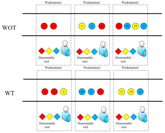
Figure 9.
Radio without considering tool deterioration.
Table 2.
Comparison of solutions with (WT) and without (WOT) tool deterioration.
The A2C produces identical results to CPLEX in the first five cases, with similar calculation times from Table 3 and Table 4. However, CPLEX has lost its runtime advantage and no feasible solution has been found, while A2C remains effective in large-scale scenarios. Comparing Table 4 and Table 5 in the first five examples by employing the same algorithm parameters to solve equivalent scenarios yields identical outcomes for both algorithms, with the A2C demonstrating faster execution. In the last large-scale case, the A2C yields superior results compared with the AC. Furthermore, compare Table 4 with Table 6, when the o-A2C and A2C algorithms are configured with the same parameters, the o-A2C approach can only obtain solutions within a narrow range and fails to acquire satisfactory solutions for medium- to large-scale scenarios.
Table 3.
CPLEX performance in considering WT.
Table 4.
A2C performance in considering WT.
Table 5.
AC performance in considering WT.
Table 6.
o-A2C performance in considering WT.
In Case 4, both algorithms achieve the same objective value of 78 with the same parameter configuration. The selected algorithm demonstrates a runtime of 2.13 s, shorter than the 2.34 s required by the AC. Figure 10 illustrates the convergence of the two algorithms across four distinct cases. These four different situations correspond from top to bottom and from left to right to the radio, kettle, washing machine, and ballpoint pen, respectively. It is evident that the A2C converges more rapidly than the AC. Specifically, from the two graphs in Figure 10 on the left, it can be seen that A2C achieves the same feasible solution as AC within 100 iterations, while AC requires approximately 150 iterations to converge.
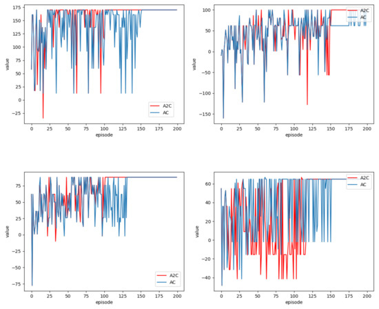
Figure 10.
Algorithm convergence.
In the case of the large-scale Case 6, our algorithm achieved an optimal target value of 333 within a runtime of 6.12 seconds. In contrast, the AC took 7.7 seconds to find a suboptimal target value of 348 (with our objective being minimization). The superiority of the A2C is showcased not only in terms of runtime but also in terms of target quality. Figure 11 provides a comparison between the optimized A2C, the original A2C (o-A2C), and the AC. The results further validate the superiority and feasibility of the optimized A2C, whilst o-A2C exhibits poor convergence.
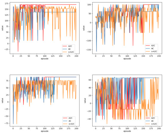
Figure 11.
Algorithm convergence.
In conclusion, in this case, the optimized A2C demonstrates a superior convergence ability compared with the o-A2C and outperforms the AC in terms of performance and problem-solving capabilities.
5. Conclusions
This paper mainly introduces the practical problem of using the A2C algorithm to solve DLBP. The work incorporates the complete disassembly method in DLBP, taking the impact of disassembly tool degradation on time into account and aiming to minimize the cycle time of workstations. The study thoroughly explores how agents use reinforcement learning algorithms to tackle DLBP. To address these concerns, a series of comparative experiments were conducted. Firstly, the results achieved using the A2C were compared with those obtained from the CPLEX solver. The results demonstrate the A2C’s efficacy in finding optimal solutions. Additionally, a comparison of A2C with AC in practical disassembly cases reveals both algorithms’ ability to find optimal solutions within a limited range, but A2C requires less time. In larger-scale scenarios, the A2C not only outperforms the AC in terms of speed but also delivers superior results in solution quality. The experimental results show that the o-A2C algorithm not only performs worse in terms of solution quality than the A2C algorithm but also cannot guarantee convergence.
In future work, we aim to enhance the algorithm’s performance by reducing the action space and minimizing the selection of prohibited actions, thereby accelerating its execution speed. Additionally, we will explore the applicability of alternative machine learning algorithms in solving DLBP problems and further improve the performance of the A2C to achieve significant enhancements [37,38,39,40,41,42,43].
Author Contributions
Writing—original draft preparation, S.Q. and X.X.; Writing—review & editing, S.Q., J.W. and X.G.; Supervision, L.Q. and W.C.; Data curation, Y.T.; Visualization, Q.T.A.T. All authors have read and agreed to the published version of the manuscript.
Funding
This work is supported in part by Liaoning Province Education Department Scientific Research Foundation of China under Grant JYTQN2023366; and in part by the Natural Science Foundation of Shandong Province under Grant ZR2019BF004.
Data Availability Statement
In accordance with MDPI’s research data policy, we hereby declare that the data utilized and generated throughout the research process are thoroughly integrated into the paper, and the data presented in the paper have been adequately furnished and duly cited.
Conflicts of Interest
The authors declare no conflicts of interest.
References
- Cao, J.; Xia, X.; Wang, L.; Zhang, Z.; Liu, X. A novel multi-efficiency optimization method for disassembly line balancing problem. Sustainability 2019, 11, 6969. [Google Scholar] [CrossRef]
- Xia, X.; Li, J.; Tian, H.; Zhou, Z.; Li, H.; Tian, G.; Chu, J. The construction and cost-benefit analysis of end-of-life vehicle disassembly plant: A typical case in China. Clean Technol. Environ. Policy 2016, 18, 2663–2675. [Google Scholar] [CrossRef]
- Ren, Y.; Jin, H.; Zhao, F.; Qu, T.; Meng, L.; Zhang, C.; Zhang, B.; Wang, G.; Sutherland, J. A multiobjective disassembly planning for value recovery and energy conservation from end-of-life products. IEEE Trans. Autom. Sci. Eng. 2020, 18, 791–803. [Google Scholar] [CrossRef]
- Qi, L.; Su, Y.; Zhou, M. A State-Equation-Based Backward Approach to a Legal Firing Sequence Existence Problem in Petri Nets. IEEE Trans. Syst. Man Cybern. Syst. 2023, 53, 4968–4979. [Google Scholar] [CrossRef]
- Xiang, D.; Lin, S.; Wang, X.; Liu, G. Checking missing-data errors in cyber-physical systems based on the merged process of Petri nets. IEEE Trans. Ind. Inform. 2022, 19, 3047–3056. [Google Scholar] [CrossRef]
- McGovern, S.M.; Gupta, S.M. A balancing method and genetic algorithm for disassembly line balancing. Eur. J. Oper. Res. 2007, 179, 692–708. [Google Scholar] [CrossRef]
- Koller, J.; Daniel, K.; Frank, D. Supporting Disassembly in Remanufacturing with Augmented Reality. In Proceedings of the 2020 IEEE International Conference on Technology Management, Operations and Decisions (ICTMOD), Marrakech, Morocco, 24–27 November 2020; pp. 1–8. [Google Scholar]
- Zhao, Z.; Liu, S.; Zhou, M.; Guo, X.; Qi, L. Decomposition Method for New Single-Machine Scheduling Problems From Steel Production Systems. IEEE Trans. Autom. Sci. Eng. 2020, 17, 1376–1387. [Google Scholar] [CrossRef]
- Gao, K.; He, Z.; Huang, Y.; Duan, P.; Suganthan, P. A survey on meta-heuristics for solving disassembly line balancing, planning and scheduling problems in remanufacturing. Swarm Evol. Comput. 2020, 57, 100719. [Google Scholar] [CrossRef]
- Guo, X.; Zhang, Z.; Qi, L.; Liu, S.; Tang, Y.; Zhao, Z. Stochastic Hybrid Discrete Grey Wolf Optimizer for Multi-objective Disassembly Sequencing and Line Balancing Planning in Disassembling Multiple Products. IEEE Trans. Autom. Sci. Eng. 2022, 19, 1744–1756. [Google Scholar] [CrossRef]
- Guo, X.; Zhou, M.; Alsokhiry, F.; Sedraoui, K. Disassembly sequence planning: A survey. IEEE/CAA J. Autom. Sin. 2021, 8, 1308–1324. [Google Scholar] [CrossRef]
- Zhao, J.; Liu, S.; Zhou, M.; Guo, X.; Qi, L. Modified cuckoo search algorithm to solve economic power dispatch optimization problems. IEEE/CAA J. Autom. Sin. 2018, 5, 794–806. [Google Scholar] [CrossRef]
- Guo, X.; Wei, T.; Wang, J.; Liu, S.; Qin, S.; Qi, L. Multi-objective U-shaped Disassembly Line Balancing Problem Considering Human Fatigue Index and An Efficient Solution. IEEE Trans. Comput. Soc. Syst. 2022, 10, 2061–2073. [Google Scholar] [CrossRef]
- Chen, J.; Chen, Y.; Chen, T.; Yang, Y. An adaptive genetic algorithm-based and AND/OR graph approach for the disassembly line balancing problem. Eng. Optim. 2022, 54, 1583–1599. [Google Scholar] [CrossRef]
- Ali, A.; Enyoghasi, C.; Badurdeen, F. A quantitative approach for product disassemblability assessment. In Role of Circular Economy in Resource Sustainability; Springer: Cham, Switzerland, 2022; pp. 73–84. [Google Scholar]
- Zhao, J.; Liu, S.; Zhou, M.; Guo, X.; Qi, L. An improved binary cuckoo search algorithm for solving unit commitment problem—Part I: Method Description. IEEE Access 2018, 6, 43535–43545. [Google Scholar] [CrossRef]
- Tan, Y.; Zhou, M.; Zhang, Y.; Guo, X.; Qi, L.; Wang, Y. Hybrid scatter search algorithm for optimal and energy-efficient steelmaking-continuous casting. IEEE Trans. Autom. Sci. Eng. 2020, 17, 1814–1828. [Google Scholar] [CrossRef]
- Tan, Y.; Zhou, M.; Wang, Y.; Guo, X.; Qi, L. A hybrid MIP-CP approach to multi-stage scheduling problem in continuous casting and hot rolling processes. IEEE Trans. Autom. Sci. Eng. 2018, 16, 1860–1869. [Google Scholar] [CrossRef]
- Li, H.; Gao, K.; Duan, P.-Y.; Li, J.-Q.; Zhang, L. An Improved Artificial Bee Colony Algorithm With Q-Learning for Solving Permutation Flow-Shop Scheduling Problems. IEEE Trans. Syst. Man Cybern. Syst. 2023, 53, 2684–2693. [Google Scholar] [CrossRef]
- Seliger, G.; Basdere, B.; Keil, T.; Rebafka, U. Innovative processes and tools for disassembly. CIRP Ann. 2002, 51, 37–40. [Google Scholar] [CrossRef]
- Fu, Y.P.; Ma, X.M.; Gao, K.Z.; Li, Z.W.; Dong, H.Y. Multi-objective home health care routing and scheduling with sharing service via a problem-specific knowledge based artificial bee colony algorithm. IEEE Trans. Intell. Transp. Syst. 2023, 25, 1706–1719. [Google Scholar] [CrossRef]
- Zhang, W.; Wang, J.; Lan, F. Dynamic hand gesture recognition based on short-term sampling neural networks. IEEE/CAA J. Autom. Sin. 2021, 8, 110–120. [Google Scholar] [CrossRef]
- Hu, B.; Wang, J. Deep learning based hand gesture recognition and UAV flight controls. Int. J. Autom. Comput. 2020, 17, 17–29. [Google Scholar] [CrossRef]
- Heng, X.; Wang, Z.; Wang, J. Human activity recognition based on transformed accelerometer data from a mobile phone. Int. J. Commun. Syst. 2016, 29, 1981–1991. [Google Scholar] [CrossRef]
- Han, H.; Li, W.; Wang, J.; Qin, G.; Qin, X. Enhance explainability of manifold learning. Neurocomputing 2022, 500, 877–895. [Google Scholar] [CrossRef]
- Ji, Y.J.; Liu, S.X.; Zhou, M.C.; Zhao, Z.Y.; Guo, X.W.; Qi, L. A machine learning and genetic algorithm-based method for predicting width deviation of hot-rolled strip in steel production systems. Inf. Sci. 2022, 589, 360–375. [Google Scholar] [CrossRef]
- Zhou, M.; Liu, S. Iterated Greedy Algorithms for Flow-shop Scheduling Problems: A Tutorial. IEEE Trans. Autom. Sci. Eng. 2021, 19, 1941–1959. [Google Scholar] [CrossRef]
- Mete, S.; Serin, F. A Reinforcement Learning Approach for Disassembly Line Balancing Problem. In Proceedings of the 2021 International Conference on Information Technology (ICIT), Amman, Jordan, 14–15 July 2021; pp. 424–427. [Google Scholar]
- Tuncel, E.; Zeid, A.; Kamarthi, S. Solving large scale disassembly line balancing problem with uncertainty using reinforcement learning. J. Intell. Manuf. 2014, 25, 647–659. [Google Scholar] [CrossRef]
- Everett, M.; Chen, Y.; How, J. Motion planning among dynamic, decision-making agents with deep reinforcement learning. In Proceedings of the 2018 IEEE/RSJ International Conference on Intelligent Robots and Systems (IROS), Madrid, Spain, 1–5 October 2018; pp. 3052–3059. [Google Scholar]
- Woo, S.; Sung, Y. Dynamic action space handling method for reinforcement learning models. J. Inf. Process. Syst. 2020, 16, 1223–1230. [Google Scholar]
- Guo, X.; Liu, S.; Zhou, M.; Tian, G. Dual-objective program and scatter search for the optimization of disassembly sequences subject to multi-resource constraints. IEEE Trans. Autom. Sci. Eng. 2018, 15, 1091–1103. [Google Scholar] [CrossRef]
- Zhao, Z.; Liu, S.; Zhou, M.; Abusorrah, A. Dual-objective mixed integer linear program and memetic algorithm for an industrial group scheduling problem. IEEE/CAA J. Autom. Sin. 2020, 8, 1199–1209. [Google Scholar] [CrossRef]
- Guo, X.; Liu, S.; Zhou, M.; Qi, L. Disassembly sequence optimization for large-scale products with multiresource constraints using scatter search and Petri nets. IEEE Trans. Cybern. 2016, 46, 2435–2446. [Google Scholar] [CrossRef]
- Wang, J. Patient flow modeling and optimal staffing for emergency departments: A Petri net approach. IEEE Trans. Comput. Soc. Syst. 2022, 10, 2022–2032. [Google Scholar] [CrossRef]
- Sutton, R.S.; McAllester, D.; Singh, S.; Mansour, Y. Policy gradient methods for reinforcement learning with function approximation. Adv. Neural Inf. Process. Syst. 1999, 12, 1057–1063. [Google Scholar]
- Zheng, L.; Wang, J.; Sheriff, A.; Chen, X. Hospital Length of Stay Prediction with Ensemble Methods in Machine Learning. In Proceedings of the International Conference on Cyber-physical Social Intelligence, Beijing, China, 18–20 December 2021. [Google Scholar]
- Du, Y.; Zhang, T.; Wang, J. Discrete Spatial Data Reconstruction based on Deep Neural Network. In Proceedings of the IEEE International Conference on Network, Sensing and Control, Banff, AB, Canada, 9–11 May 2019. [Google Scholar]
- Zhang, W.; Wang, J. Dynamic Hand Gesture Recognition Based on 3D Convolutional Neural Networks Models. In Proceedings of the IEEE International Conference on Network, Sensing and Control, Banff, AB, Canada, 9–11 May 2019. [Google Scholar]
- Asan, A.S.; Kang, Q.; Oralkan, O.; Sahin, M. Entrainment of cerebellar Purkinje cell spiking activity using pulsed ultrasound stimulation. Brain Stimul. 2021, 14, 598–606. [Google Scholar] [CrossRef]
- Wang, Y.; Kang, Q.; Zhang, Y.; Liu, X. Optically computed optical coherence tomography for volumetric imaging. Opt. Lett. 2020, 45, 1675–1678. [Google Scholar] [CrossRef] [PubMed]
- Javan-Khoshkholgh, A.; Kang, Q.; Abumahfouz, N.; Farajidavar, A. Monitoring and Modulating the Gastrointestinal Activity: A Wirelessly Programmable System with Impedance Measurement Capability. Annu. Int. Conf. IEEE Eng. Med. Biol. Soc. 2019, 2019, 1127–1130. [Google Scholar] [CrossRef] [PubMed]
- Alrofati, W.; Javan-Khoshkholgh, A.; Bao, R.; Kang, Q.; Mahfouz, N.A.; Farajidavar, A. A Configurable Portable System for Ambulatory Monitoring of Gastric Bioelectrical Activity and Delivering Electrical Stimulation. Annu. Int. Conf. IEEE Eng. Med. Biol. Soc. 2018, 2018, 2829–2832. [Google Scholar] [CrossRef] [PubMed]
Disclaimer/Publisher’s Note: The statements, opinions and data contained in all publications are solely those of the individual author(s) and contributor(s) and not of MDPI and/or the editor(s). MDPI and/or the editor(s) disclaim responsibility for any injury to people or property resulting from any ideas, methods, instructions or products referred to in the content. |
© 2024 by the authors. Licensee MDPI, Basel, Switzerland. This article is an open access article distributed under the terms and conditions of the Creative Commons Attribution (CC BY) license (https://creativecommons.org/licenses/by/4.0/).