1. Introduction
Electroencephalographic (EEG) signals measure the electrical activity related to cerebral functioning [
1]. Recently, research based on EEG signals has provided a better understanding of brain functioning [
2], allowing accurate diagnoses and cerebral disease treatments [
3,
4]. Moreover, the processing and classification of EEG signals are of great importance for medical analyses and Brain–Computer Interface (BCI) applications; for example, to control devices [
5] and to improve the quality of people’s lives [
6]. Nowadays, various EEG-BCI systems are based on executed and imagined movements, offering an extensive range of solutions to assist people in daily life. Cho et al. [
7] controlled a robot hand using EEG signals recorded by performing and imagining hand movements. They reported average classification accuracies of 56.83% for Motor Execution (ME), and 51.01% for Motor Imagery (MI), respectively, using the Common Spatial Patterns (CSP) and the Regularized Linear Discriminant Analysis (RLDA) algorithms. For their part, Demir Kanik et al. [
8] decoded the upper limb movement intentions before and during the movement execution, adding MI to ME trials. Their framework aimed to improve ME classification for robot control. Traditionally, the effectiveness of an EEG-based BCI system relies on the accurate classification of brain signals, which depends on how features extracted from raw data are distinguishable. Therefore, the EEG feature extraction challenge becomes far more complex considering the EEG’s non-stationary nature and the artifacts caused by the body’s muscular activity.
In the recent literature, various techniques have been used to efficiently differentiate ME and MI features. For example, Thomas et al. [
9] investigated parameters associated with ME and MI of left/right-hand movements using the CSP algorithm. They drew conclusions on the suitability of the frontal and parietal channels discriminating ME and MI tasks, with an average accuracy of 81%. In another work, Usama et al. [
10] evaluated the Error-related Potentials (ErrP) decoding by combining ME and MI features of right–left wrist extensions and foot dorsiflexion. For that purpose, 89 ± 9 and 83 ± 9% accuracies were obtained using the random forest classifier. Such results showed significant inter-subject variability, detecting ErrPs from temporal features. Recently, a BCI-Transfer learning based-Relation Network (BTRN) allowed the decoding of MI and ME tasks, applying a transfer learning architecture to discriminate high-complexity features [
11]. Definitely, ME and MI feature discrimination help establish their correlation, neurological similarity, and divergence. This analysis is of the utmost importance, especially for BCI applications, where exploiting either paradigm can improve the hoped-for results.
Recent studies have reported a parallel sensorimotor cortex activation caused by ME and MI tasks [
12,
13]. However, distinguishing between EEG features related to ME and MI tasks remains challenging for BCI-based paradigms. Therefore, the sensorimotor rhythm similarity between ME and MI depends essentially on the subject MI ability, as concluded by Toriyama et al. [
13]. Furthermore, the inter-subject variability of BCI efficiency according to paradigms and sessions, well known in the associated literature as BCI illiteracy, explains that a considered subject can perform better in one specific task but not another [
14].
Recently, Hardwick et al. [
15] proposed a quantitative synthesis for MI, such as an action observation and ME neural correlation. Based on neuroimaging experiments, different mental tasks provoke particular activations in specific brain areas. In the same sense, Matsuo et al. [
16] investigated cerebral hemodynamics during the ME and MI of a self-feeding task employing chopsticks to emphasize varied levels of brain activation in some areas during ME and MI tasks. In the recent past, techniques such as successive decomposition index [
17], transfer learning [
11], frequency-band power analysis [
13], and Filter Bank Common Spatial Pattern (FBCSP) [
18] have been frequently used to discriminate ME from MI features for BCI-based systems. However, from a general point of view, machine learning approaches demonstrated significant advantages in analyzing ME and MI deep features to be classified.
On the other hand, Hjorth et al. [
19] introduced three parameters based on variance properties to analyze features of EEG curves using a time-based calculation. These parameters are activity, mobility, and complexity. Activity measures the square of EEG amplitude standard deviation, in other words, the variance of EEG signals in a considered window. Mobility is defined as the average power of the normalized derivative of EEG signals. At the same time, complexity represents the ratio between EEG mobilities, i.e., the first derivative’s mobility, and EEG signals’ mobility. In sum, several approaches have been proposed in the recent literature to accurately discriminate ME and MI EEG tasks for BCI applications [
12,
20,
21,
22]. Therefore, it is hypothesized in the present framework that ME and MI EEG features are distinguishable by gainfully employing the aforenamed Hjorth parameters.
This work aims to discriminate EEG features between ME and MI movements using the fast fixed-point algorithm for Fast Independent Component Analysis (FastICA) [
23,
24], Hjorth parameters, and the Support Vector Machines (SVMs) classifier. Consequently, four preprocessing steps were implemented as follows. First, frequency-band filters were applied to reduce undesired frequency components. Next, sources were estimated using the FastICA algorithm to determine components with increased electrical activity in the brain cortex areas. Then, both filtered and unfiltered features were extracted using the Hjorth parameters based on the activity, mobility, and complexity of EEG signals. In the last step, the SVM classifier discriminates and classifies the EEG segments related to ME and MI tasks.
Mainly, the paper’s contributions are summarized as follows.
Reliable discrimination between ME and MI features considering both filtered and unfiltered EEG signals.
A method based on Machine Learning combining FastICA, Hjorth parameters, and SVM algorithms is proposed.
Two classification approaches to discriminate ME and MI tasks were accurately developed.
This paper is organized as follows.
Section 2 summarizes recent works related to the topic. The methods used in this framework are presented in
Section 3, emphasizing the dataset description and signal processing steps.
Section 4 obtained and discusses the achieved numerical results. Finally,
Section 5 formulates the conclusions of this work.
2. Related Works
Numerous works have been proposed to discriminate among features in the recent literature related to ME and MI features classification for BCI systems. Long before, Sleight et al. [
20] analyzed features carried by EEG frequency bands to distinguish executed and imagined segments. They reported average classification accuracies of 56.0% using ICA and SVM, classifying features from C3, C4, and Cz channels. In another work, Alomari et al. [
12] analyzed EEG signals corresponding to executed and imagined fist movements for BCI applications. They used Wavelet Transform (WT) and an approach-based machine learning. Average classification accuracies of 81.5 and 88.93% were achieved with their framework, discriminating ME and MI of left–right fist tasks, respectively. Besides, ME and MI movements of the fists have been discriminated against using the power spectrum analysis of the Dynamic Mode Decomposition (DMD) components [
21]. The highest reported accuracy was about 83%, utilizing an SVM classifier with a linear kernel function.
Furthermore, pattern recognition and categorization of ME and MI for one-hand finger movements were proposed by Sonkin et al. [
25], using artificial neural network (ANN) and SVM models. Higher accuracies of 42% and 62% were obtained by decoding ME and MI of the thumb and index fingers. For their part, Baravalle et al. [
26] analyzed EEG signals of the right and left hands, using emergent dynamical properties, wavelet decomposition, and entropy–complexity plane to distinguish ME from MI tasks. Their results allowed the quantification of intrinsic features corresponding to ME and MI tasks. Recently, Chen et al. [
27] investigated how to increase the number of commands for BCI systems by using ME and MI of left–right gestures. They used hierarchical SVM (hSVM) to distinguish ME and MI tasks, achieving an average accuracy of 74.08 ± 7.29% through five-fold Cross-Validation (CV).
On the other hand, numerous datasets based on ME and MI EEG signals have been published [
28,
29]. In this sense, Schalk et al. [
30] proposed a development platform named BCI2000 for applications-based BCI general purpose, in addition to releasing a large EEG ME-MI database. Since then, numerous scientific researchers have employed EEG data from the Physionet database to implement BCI systems and test algorithms.
Table 1 summarizes recent works on ME and MI task discrimination.
3. Materials and Methods
This work aims to classify ME and MI EEG signals provided by the Physionet dataset. In this sense, the preprocessing step contemplates three stages. First, C3, Cz, C4, F3, Fz, F4, P3, Pz, and P4 channels are selected from the provided 64 channels according to the defined tasks because of their spatial location on the brain cortices [
31,
32]. Next, sub-band filtering is applied to constitute theta (
), alpha (
), and beta (
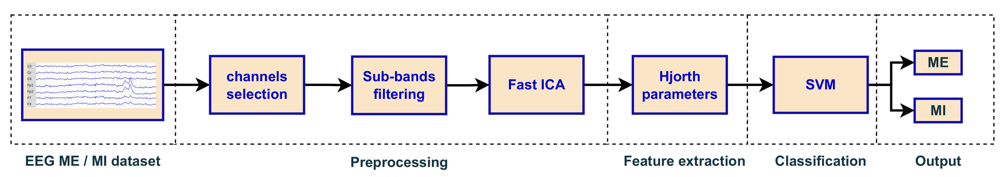
) sub-band data. The last preprocessing stage uses the FastICA algorithm to separate independent sources from raw EEG signals and sub-band data. For the features extraction step, Hjorth criteria are employed to extract ME and MI features, reducing the complexity of EEG data. Finally, the SVM classifies patterns resulting from the Hjorth parameters combination. Concretely, patterns maximizing the distance from the optimal hyperplane to the nearest point of each pattern are classified as ME or MI, to give the output.
Figure 1 presents the overview of the proposed method, contemplating the aforementioned steps.
3.1. The Physionet Dataset
The proposed method utilizes EEG data from the Physionet dataset [
30,
33]. This dataset contains ME and MI signals from 64 channels in the EDF+ format, representing 160 samples per second and channel. Besides, an annotation is given about the baseline record. Thus, 109 volunteers were labeled from S001 to S109 and performed 1526 records of ME and MI activities. Globally, 14 experimental runs were executed per subject: 2 one-minute baseline runs with eyes opened and closed each, and 3 two-minute the others. A detailed description of the experimental procedure is given in
Table 2.
Therefore, T1 and T2 codes are assigned to the class “executed” in tasks R03, R05, R07, R09, R11, and R13. Whilst T1 and T2 codes correspond to the class “imagined” in tasks R04, R06, R08, R10, R12, and R14. Exceptionally, EEG recordings corresponding to volunteers S088, S089, S092, S100, S104, and S106 were removed from the dataset due to irregular and unpredictable variations. In summary, 14 experimental runs were executed with the remaining 103 volunteers. Hence, EEG data to be processed contain or 1442 EEG records per channel.
3.2. Channel Selection
Current channel selection approaches include the correlation coefficient evaluation, Common Spatial Pattern (CSP), sequential-based algorithm, and binary particle swarm optimization-based algorithm methods [
34]. However, in the specific case of ME and MI tasks, the related literature is unanimous that the Supplementary Motor Area (SMA), the Premotor Cortex (PMC), and the primary motor cortex (M1) are significantly activated during both ME and MI [
35,
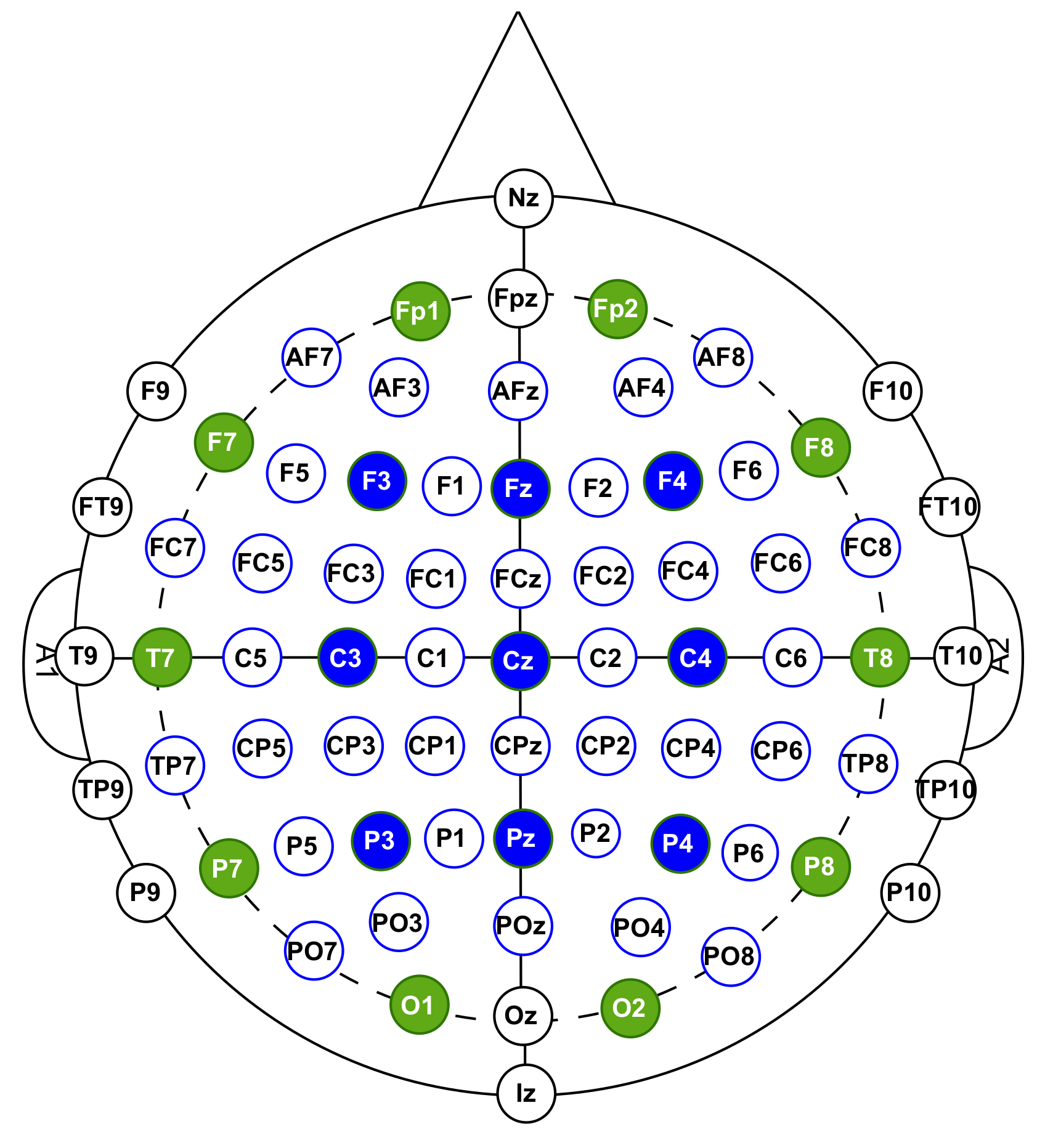
36]. Therefore, two steps were implemented to select channels in this work. As a first approach, 19 channels corresponding to the 10-20 electrode placement system were considered from the 64 provided by the referred dataset, i.e., C3, Cz, C4, Fp1, Fp2, F7 F3, Fz, F4, F8, T7, T8, P7, P3, Pz, P4, P8, O1, and O2 channels. Such a channel selection was made considering two significant aspects. On the one hand, selecting a few channels reduces the processing time and computational resources by considering only discriminant signals, as reported by Baig et al. [
37]. On the other hand, the 10–20 electrode placement system offers a good channel spatial resolution to evaluate the selected channel set contribution according to the defined paradigms [
38]. In addition, the channels above were selected to evaluate their contribution, considering the conclusions formulated in [
39,
40] about the parallel activation of various cortices caused by one or various stimuli.
Figure 2 shows the 19 considered channels for the proposed framework.
3.3. Sub-Band Filtering
In total, 8652 EEG segments were decomposed in three sub-bands to analyze their intrinsic features. The proposed approach considers filtering EEG signals in theta (
), alpha (
), and beta (
) sub-bands, according to the literature related to ME and MI tasks, the defined paradigm, and the age of participants [
9,
41]. EEG signals in sub-band delta (
∈ [0.5, 4] Hz) appear in deep dreamless sleep, loss of body awareness, quietness, lethargy, or fatigue. For this cause, the delta sub-band is not considered in the case of ME and MI tasks [
42]. Therefore, fifth-order Chebyshev type II band-pass filters were applied to obtain 4–8, 8–13, and 13–30 Hz sub-bands for
,
, and
bands, respectively. Sub-band filters were designed by specifying a stop band attenuation at −34 dB. In this sense, the filter transition bands reached 80% of the gain, considering that the pass-band frequency ranges are different for
,
, and
waves.
3.4. FastICA
A noise reduction step was performed using the FastICA algorithm to deal with artifact problems and undesirable signals carried in EEG data [
22,
43]. The FastICA algorithm and its variants are commonly used for denoising biomedical signals from muscular artifacts [
44], especially in enhancing EEG signals [
45]. In addition, FastICA offers a dimensionality reduction of classification problems for independent observations, making it more suitable for practical implementation [
46]. Concretely, the implemented FastICA-based denoising approach decomposes signals from 19 channels into 19 independent components. It is assumed that the number of independent components equals the number of channels to meet at least one of the FastICA algorithm constraints. At long last, the independent components with greater energy concentration were selected.
Formally, let us express an input signal vector
, such as a linear combination of the mixture matrix
and the noisy matrix
to be removed. Here,
is constituted to maximize the utility metric by combining channels with relevant information [
47]. That is to say,
To this, the input signals must be centered. Next, the whitening process converts the mixture matrix
into a new orthogonal whitened matrix
as follows
where
V is an orthogonal matrix (eigenvectors of
),
is the diagonal matrix of eigenvalues, and
is the whitened signal. The FastICA quests the appropriate direction for the weight vector
W that maximizes the non-Gaussianity of the
projection with the extraction purpose of Independent Components (ICs).
FastICA uses the non-linear function
and its first (
3) and second (
4) derivatives to measure the non-Gaussianity, such as
Finally, ICs are found according to the steps presented in Algorithm 1.
corresponds to a channel subset into the 19 preselected channels. In this work, the method essentially seeks to evaluate the ME and MI activities in the somatosensory cortex. Therefore, the
set comprised C3, Cz, C4, F3, Fz, F4, P3, Pz, and P4 channels because of their optimal location on the skull [
35,
48].
Furthermore, the criterion defined in the eighth step of Algorithm 1 specifies the threshold for an ith independent component to be selected according to the energy concentration in the selected channels.
Practically, a concentration value greater than 50% matched in independent components was not encountered, and concentrations lower than 20% resulted in poor noise suppression.Therefore, the minimal concentration of 35% for
and
rhythms in the motor brain cortex was established empirically to select half of the independent components
with an acceptable noise suppression rate.
| Algorithm 1 FastICA algorithm used to denoise EEG signals |
- 1:
Initial weight vector randomly, where p represents the number of projections. - 2:
Let − . - 3:
Apply the Gramm-Shmidt orthogonalization to the weight vectors , after the jth iteration for p projections: . - 4:
Compute the vector normalization, . - 5:
Obtain the 19 Independent Components (ICs), if converges; otherwise, , and repeat steps from 2 to 4. - 6:
Evaluate each ICs separatelfy and by sub-band, , i is the number of channels, and the sub-band EEG signals. - 7:
Criterion: Select ICs with higher average energy by sub-band, - 8:
Reconstruct EEG signals according to , where is the mixture matrix.
|
3.5. Feature Extraction
After the denoising step, the proposed method extracts EEG features by evaluating the parameters introduced by Hjorth [
19]. Namely, the data’s activity, mobility, and complexity are calculated per channel for the raw EEG vector
and for the reconstructed EEG vector
with and without sub-band decomposition. The activity represents the signal power or mean energy, obtained by calculating the signal variance as follows:
where
N is the sample length, and
denotes the mean of the signals’ amplitude. For its part, the mobility parameter
is associated with the mean frequency as follows:
where the signal derivative
is obtained by calculating the difference from two consecutive signal samples,
. Finally, EEG complexity represents how the frequency changes in comparison to a plain sine wave, calculated as follows:
Therefore, activity, mobility, and complexity of EEG data were calculated for each sub-band and without sub-band decomposition, obtaining 12 features per channel, as shown in
Table 3.
Since the ranges of feature mixtures varied considerably, especially those of activity versus mobility or complexity, it was recommended to normalize the data based on the minimum–maximum criteria to consider the limits of each range. Therefore, data features were normalized in the interval
as follows:
where
is the
ith normalized value of the
kth feature,
and
are the maximum and minimum values of the
kth feature, respectively. In sum, the Hjorth parameters helped calculate the EEG data statistical properties to constitute feature subsets, more distinguishable by the classifier [
49].
3.6. Feature Classification
An SVM-based model carries out the feature classification step. Most works related to the classification of ME and MI features in the recent literature use the SVM model. Thus, in this case, the SVM model was selected to emphasize the contribution of the preprocessing and feature extraction steps using the Hjorth parameters. The SVM model uses a Gaussian kernel given by
where
and
are vector pairs in
with
the number of features. The parameter
is inversely proportional to the influence of a vector over its neighbors. Based on studies developed by Platt [
50], the proposed margin SVM model uses the Sequential Minimal Optimization (SMO) algorithm solved by
Subject to constraints,
where
represents the pattern pairs of an input vector
and the corresponding output class label
,
M is the number of classes, and
is the Lagrange multiplier for a class m, varying between 0 and
C. Therefore, feature
and its output
are associated following their pertinence to the ME or MI movements class.
In this work, 12 features per each of the 9 considered channels were available for classification, giving a total of 108 features.Moreover, the proposed method opted for feature and channel combinations to efficiently perform the classification task, as presented in
Table 3. The proposed method was implemented in Python 3.6 on an Ubuntu 22.04 desktop with an NVIDIA GTX 1080 Ti GPU using the scikit-learn library [
51].
4. Numerical Results
This section presents the numerical results obtained using denoising, feature extraction, and classification methods, highlighting valuable observations from the signals processing chain. The reported results correspond to R03, R04, R07, R08, R11, and R12 tasks, defined previously in
Section 3.1.
4.1. Noise Suppression Using FastICA
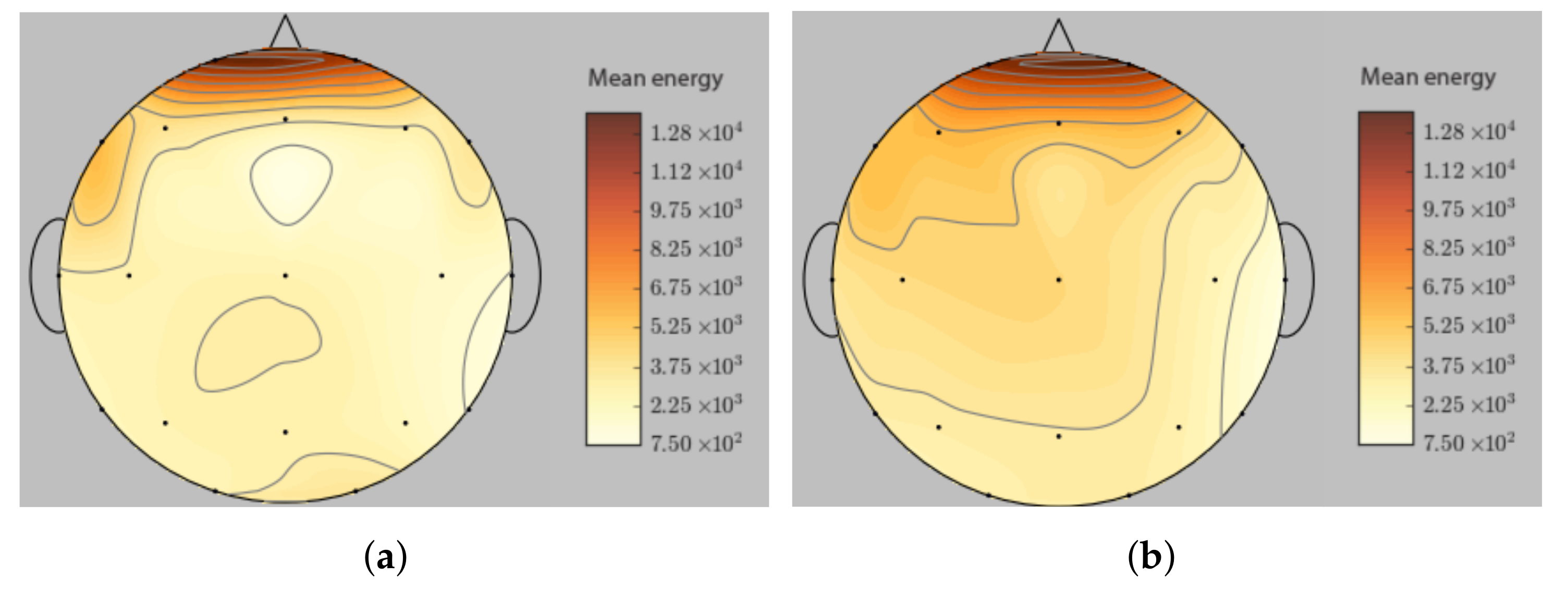
The effect of denoising EEG data is explored by analyzing the brain mapping before and after applying the FastICA algorithm, as shown in
Figure 3. It can be observed that Fp1 and Fp2 channels perceive more ocular artifacts caused by eye blinking and eye movements than other channels.
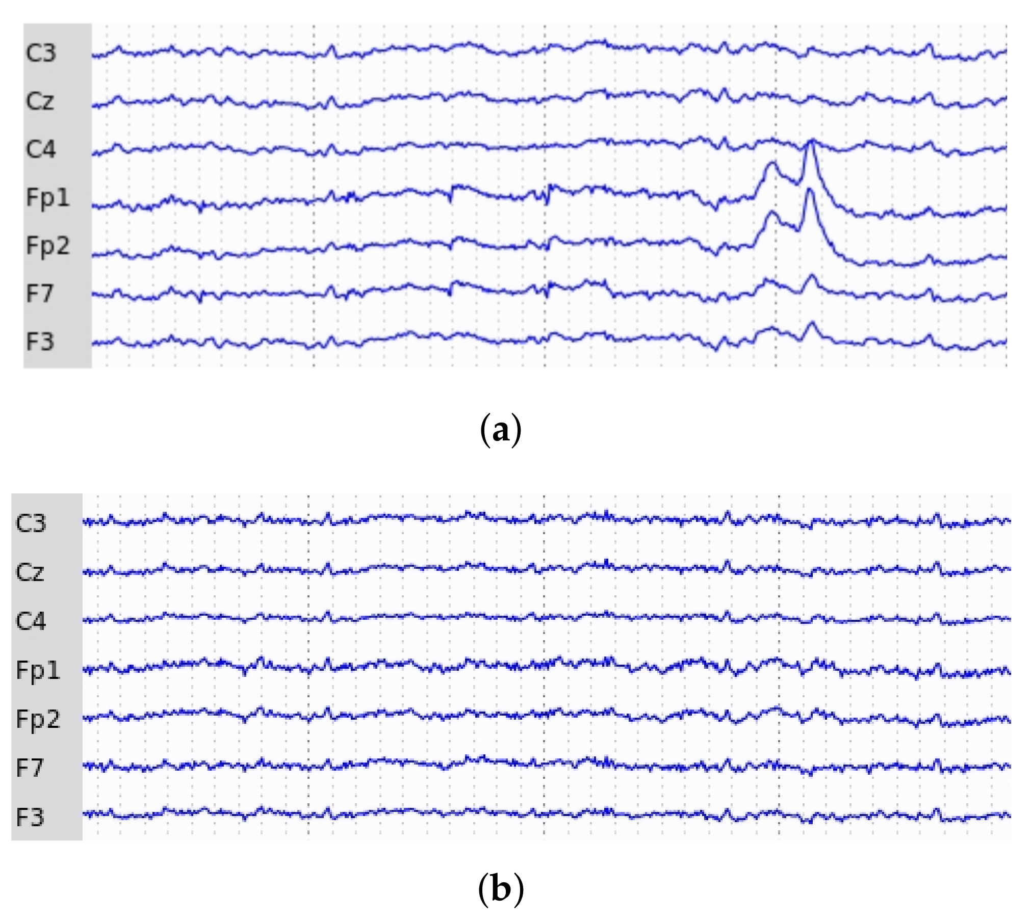
Figure 4 compares artifact reduction in C3, Cz, C4, Fp1, Fp2, F7, and F3 channels before and after the denoising step. Illustratively, R04 task signals provided by Fp1, Fp2, and F7 channels were selected to highlight the increased performances using the FastICA algorithm. In addition, analyzing EEG segments’ mean energies revealed signals denoising the benefits of the FastICA algorithm, on the sensorimotor cortex.
4.2. Features Extraction
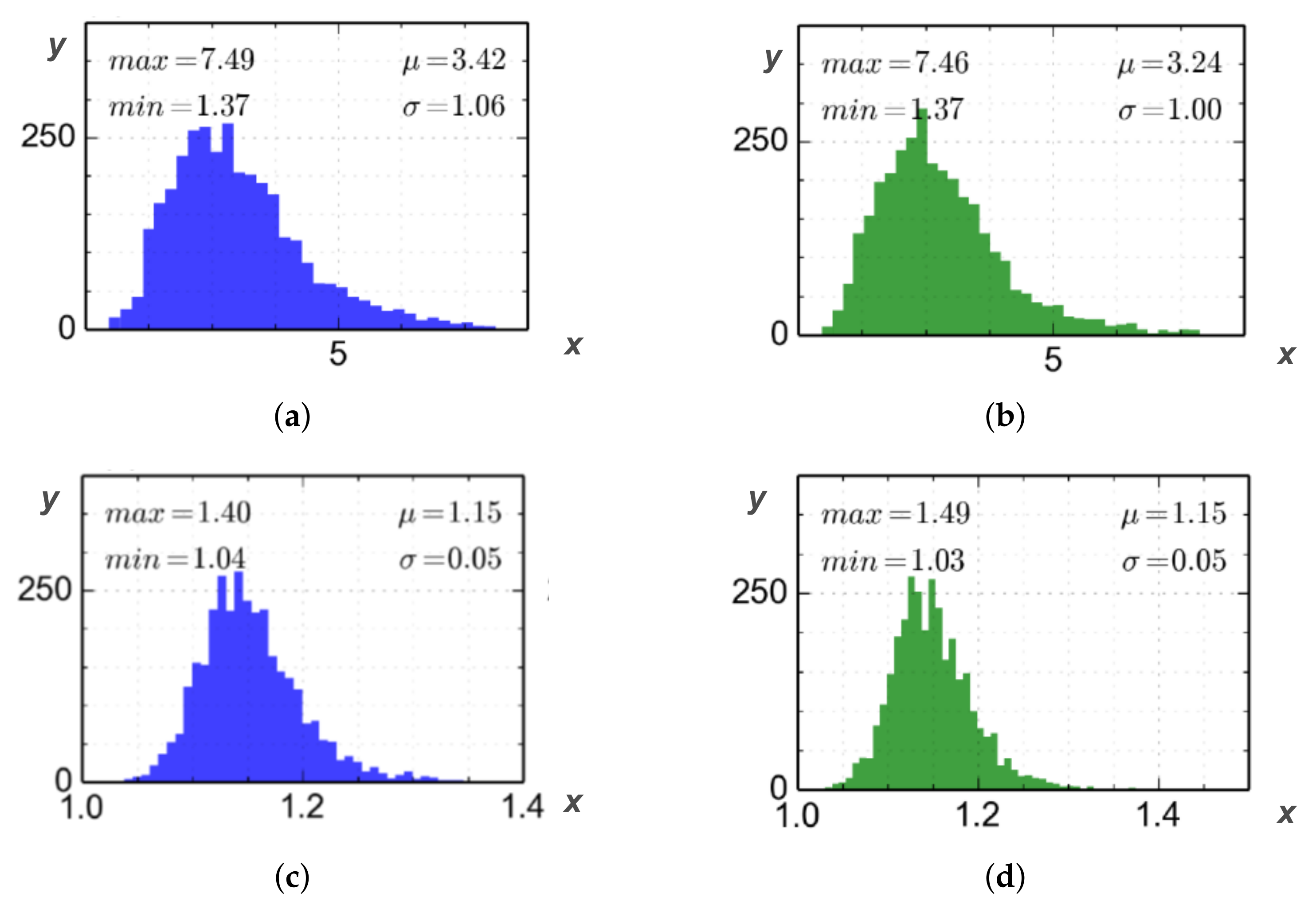
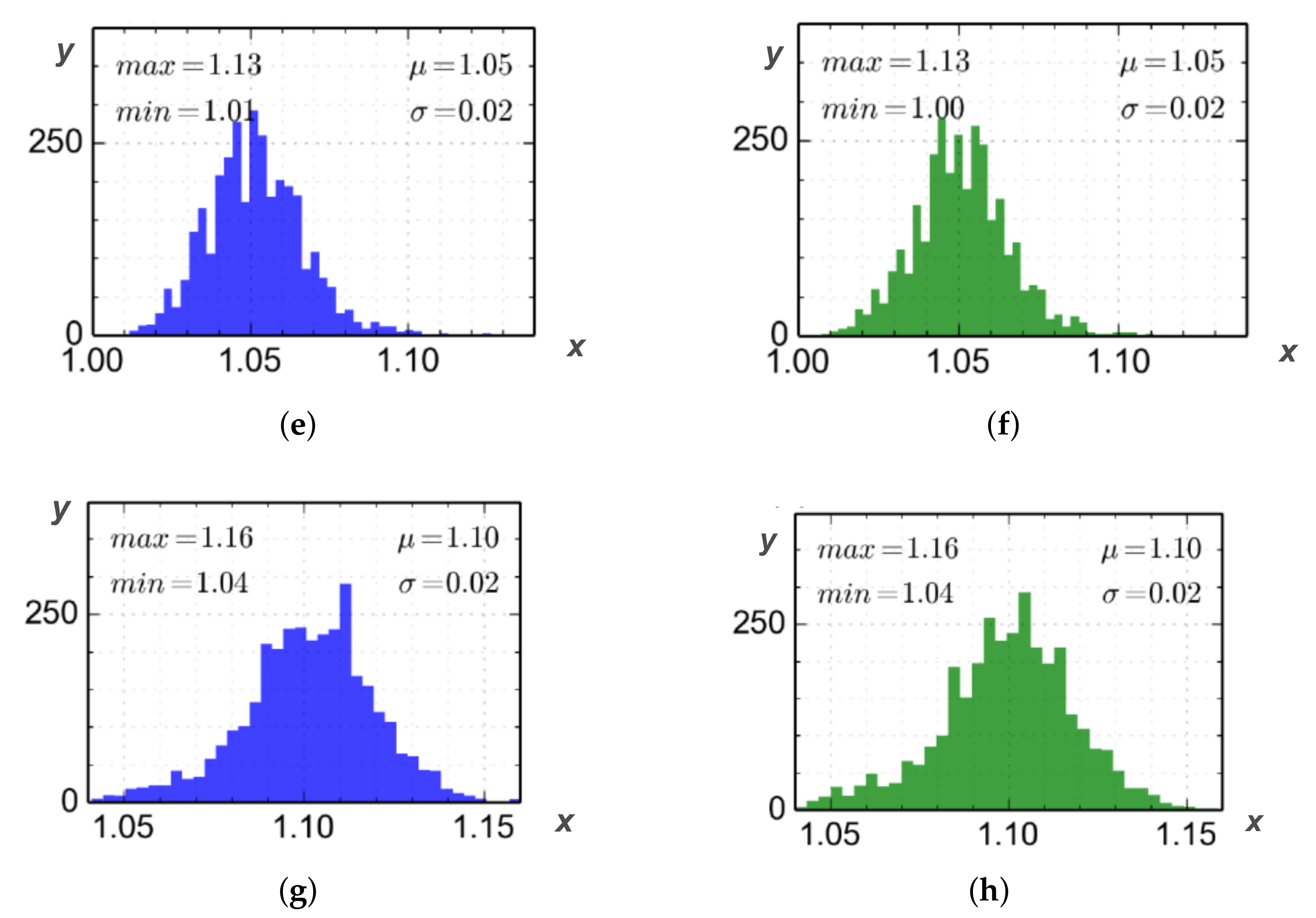
The proposed method uses histogram analysis to evaluate feature distribution using activity, mobility, and complexity descriptors. Therefore, various histograms were analyzed, considering essentially channel signals, sub-band, and raw data for both ME and MI classes. Illustratively,
Figure 5 presents the histograms corresponding to filtered and unfiltered C3 channel signals for the EEG complexity parameter.
4.3. Features Classification Evaluation
The classification step used the accuracy metric given by
where
represents the true positive for each m feature correctly assigned to class M,
corresponds to the true negative for each n feature of other classes than M unassigned to class M.
is the false positive, representing all features assigned erroneously to class M, and oppositely
represents the false negative. Additionally, the SVM classifier performance was evaluated by utilizing the confusion matrix metric [
52].
Therefore, two classification approaches were developed in this work. The first one (Method 1) is based on R03, R04, R07, R08, R11, and R12 tasks and uses signals of all subjects. That is 8652 samples from 103 subjects, 14 runs, and 6 considered tasks. In other words, the subject-independent classification approach. Therefore, samples of the first 10 runs constituted the training set; those of the 11th and 12th, and 13th and 14th runs were used as the testing and validation sets, respectively.
Table 4 summarizes data splitting for training, testing, and validation sets.
The second classification approach (Method 2) used a cross-subjects approach where samples of a determined number of subjects were utilized for training the model. In contrast, samples of others were used to test and validate the results. Thus, samples of the first 83 subjects were used to train the model, while those from the 84th to 93rd subjects served to test the model. Finally, samples from the 94th to 103rd subjects were utilized to validate the model, as reported in
Table 4. Hence, the first classification approach used 71.4%, 14.3%, and 14.3% of all data for training, testing, and validation. At the same time, the second approach utilized 80% of the data to train, 10% to test, and a further 10% to validate the model.
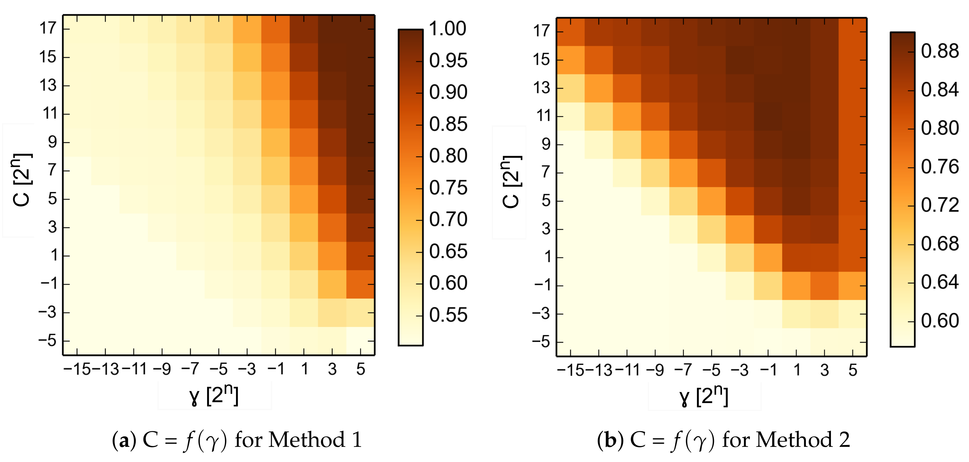
The SVM classifier was configured with a Gaussian kernel to discriminate feature combinations of ME and MI tasks, as presented in
Table 5. Different combinations of
and C parameters were explored, computing from Equations (
9)–(
11).
Figure 6 shows the explored combinations of
and C parameters to find the classifier’s optimal efficiency for both classification approaches.
Therefore,
and C parameter values were set to
and
, respectively. The reported results were averaged by running the model five times for each approach. Therefore,
Table 6 presents the ME and MI classification results using the accuracy metric followed by the standard deviation.
Moreover, the confusion matrix metric was used to evaluate the classifier performance in discriminating ME and MI tasks.
Table 7 summarizes the confusion matrices for the five feature combination sets, as considered in
Table 5. Therefore, the
and
features of C3, C4, and C5 channels were correctly discriminated with Method 1, achieving a true negative rate of 89.33% for MI tasks, against a true positive rate of 89.7% for ME tasks.
Discrimination rates of true positive (68.17%) and true negative (68.41%) were obtained with the same combination of features by using Method 2, as reported in
Table 7.
In addition, based on C3, Cz, and C4 channel selection, EEG signals were processed without either sub-band sampling or denoising steps to evaluate both the SVM classifier performance and the preprocessing benefits.
Furthermore,
Table 8 presents the comparative results of feature classification using Method 1 and Method 2 with and without denoising.
4.4. Discussion
According to
Table 6, the best classification accuracy was obtained with the
,
,
,
, and
features of C3, Cz, and C4 channels by implementing Method 1 (89.7 ± 0.78%). The same feature combination of the C3, Cz, and C4 channels gave reliable results using Method 2 (68.8 ± 0.71%). Considering the spatial location of C3, Cz, and C4 electrodes on the skull, these results confirm the hypothesis that the brain sensorimotor cortex is activated during both ME and MI tasks.
On the other hand, the combination of the
and
features allowed the best discriminant accuracy to be achieved with Method 1 rather than by using Method 2. A difference of 20.9% between both methods is essentially due to the specificity of each method. According to
Table 7, MI features have been better identified by the ICA–Hjorth–SVM method than ME features, independently of the selection of channels or feature combinations. It is important to highlight here that the key contribution of this work is both the channel and Hjorth feature combinations for raw and filtered signals. Concretely, classifying ME and MI gave different results depending on feature combinations. The features set composed of
and
allowed discriminating 79.45% of ME against 79.75% of MI with Method 1. These results were improved by combining features from all Hjorth parameters for raw and filtered data (see
Table 7).
The first classification approach (Method 1), where 10 runs were used to train and the remaining tasks to test and validate the model, was revealed to be more efficient than the second, where all data were partitioned by subject to constitute the training, testing, and validation sets (Method 2). The fact that fractions of features provided by all subjects were used in Method 1 to train, test, and validate the proposed model can justify this improvement. In other words, the model learns from the patterns of all subjects. Unlike Method 1, where the model learned from the data portion of all subjects, Method 2 used features from 83 subjects to train the model. Data from the remaining subjects were utilized to test and validate the model, respectively. This strategy would have decreased the classifier performance, considering that the testing and validation data were provided by subjects who would not performed better on the defined tasks.
For its part, the denoising process gained an accuracy increase of 17.6% and 14% in the classification of ME and MI features, using Method 1 and Method 2, respectively, than processing without denoising. Finally,
Table 9 compares the results achieved in this work with those published in the related works, considering the referred dataset.
In the model proposed by Sleight et al. [
20], ICA and non-ICA approaches were contemplated before the channel selection step. Successively, a rhythmic band selection and average power evaluation helped differentiate the ME and MI signals by employing an SVM classifier. They reported an average accuracy of 56.0 ± 0.27%, classifying EEG signals normalized in frequency bands and denoised by ICA.
For their part, Alomari et al. [
12] achieved an average accuracy of 88.9% by utilizing a combination of WT and ANN to discriminate ME and MI tasks. By analyzing the closeness between their results and those achieved in this work, Alomari et al. used a wavelet Transform Analysis to extract ME and MI features using the Daubechies orthogonal wavelets Db12. An artificial neural network designed with 15 hidden layers allowed their model to obtain the reported results without minimizing the contribution of filtering and feature extraction by the wavelet transform. Lately, a cascade of DMD and SVM has been proposed to differentiate real and imaginary fist movements, achieving an accuracy of 83% [
21].
In this work, an average accuracy of 89.7 ± 0.78% has been obtained in discriminating ME and MI features of C3, Cz, and C4 channels. The proposed method contemplated the EEG sub-band filtering, denoising, and classification steps. Therefore, this framework presents a reliable alternative for discriminating ME and MI EEG tasks for BCI-based applications.
5. Conclusions
This work aimed to classify ME and MI EEG features using sub-band filtering, noise suppression, and feature extraction algorithms. Concretely, EEG signals provided by the selected channels were filtered in , and sub-bands before being denoised by the FastICA algorithm. Thereafter, Hjorth parameters, namely, activity, mobility, and complexity were computed to extract features, discriminated next by an SVM classifier to give the output. In other words, the developed approach allowed the discrimination of ME-MI tasks by reducing non-relevant information contained in EEG data. According to the results, the activity, mobility, and complexity of EEG segments carried by C3, Cz, and C4 channels with and without sub-band decomposition gave reliable classification accuracies. Therefore, a higher average classification accuracy of 89.7 ± 0.78% was achieved with the feature combination.
Moreover, data processing without filtering and denoising steps was contemplated to highlight the overall preprocessing step benefit. In this sense, the proposed framework offers an alternative to BCI implementation for multiple users, considering the large amount of data used to experiment with the model.
However, the results reported in this work are essentially related to the combination of the features, to the Hjorth criteria, and especially to the operated splitting of data in training, testing, and evaluation sets. In future works, it is projected to compare the performance of the Hjorth algorithm coupled to FastICA method variants by implementing the proposed model on development boards, namely, FPGA and NVIDIA developer cards for embedded BCI systems.


 ,
, 
