Developing New Fully Connected Layers for Convolutional Neural Networks with Hyperparameter Optimization for Improved Multi-Label Image Classification

Abstract

Chest X-ray evaluation is challenging due to its high demand and the complexity of diagnoses. In this study, we propose an optimized deep learning model for the multi-label classification of chest X-ray images. We leverage pretrained convolutional neural networks (CNNs) such as VGG16, ResNet 50, and DenseNet 121, modifying their output layers and fine-tuning the models. We employ a novel optimization strategy using the Hyperband algorithm to efficiently search the hyperparameter space while adjusting the fully connected layers of the CNNs. The effectiveness of our approach is evaluated on the basis of the Area Under the Receiver Operating Characteristic Curve (AUC-ROC) metric. Our proposed methodology could assist in automated chest radiograph interpretation, offering a valuable tool that can be used by clinicians in the future.

1. Introduction

The chest radiograph (CXR) is one of the most common medical imaging examinations in the world. Using only a small dose of radiation, this examination has the potential to discover conditions that require urgent care, e.g., pneumothorax and pneumonia, which can be fatal in children in developing countries and in older patients in developed countries. According to the WHO, four million people die from pneumonia each year, representing a mortality rate of 0.88% of the 450 million annual pneumonia cases [1]. Although the mortality rate may seem low, it is alarming to note that pneumonia is responsible for 7% of deaths from all causes.

Meanwhile, the number of radiologists is increasing year by year in the US [2]; however, there are countries, for example, Liberia, where the shortage of radiologists is severe, with only two active radiologists for four million people being reported in 2015 [3].

Emergency departments (EDs) are prominent places for radiographic chest examinations, with a reportedly being used in 34.4% of ED visits [4]. There was a significant rise in the use of radiology in the diagnosis of pneumonia during the COVID-19 pandemic. However, the number of healthcare providers, such as radiologists, is not scalable. Human resource limitations cannot be quickly resolved during a crisis due to the years of training required for these professions. The increasing use of imaging in ED services has become a critical problem due to the costs and human resources required. The use of artificial intelligence in the evaluation of X-ray images can help to decrease the cost and staffing issues, while further decreasing the turnaround time for reports.

Another condition in which timely diagnosis is important is pneumothorax (PTX). PTX is a condition in which air enters between the two layers of the pleura, resulting in partial or complete collapse of the lung, which subsequently causes breathing difficulty or even respiratory failure. PTX can develop spontaneously or due to trauma of the chest cavity, both posing significant health burdens. Spontaneous pneumothorax has an annual incidence of 18–28 and 1.2–6 cases per 100,000 men and women, respectively, mainly affecting the young and elderly populations. In a bid to reduce the time to diagnosis, chest ultrasound (CUS) is becoming a more popular choice of test, even though the diagnostic yield of CUS largely depends on the operator’s expertise. An automated immediate evaluation for the presence or absence of PTX on a chest X-ray could significantly improve health outcomes and decrease human resource needs [5].

Diagnosing the diseases mentioned above as soon as possible could save millions of lives annually. Chest X-rays account for more than 40% of all X-rays. Of these millions of X-rays taken, more than one million are interpreted visually by radiologists. This procedure requires a high degree of concentration and experience. There is a need to develop computer-aided diagnostic algorithms and methods to reduce physicians’ workloads and improve diagnostic accuracy. The emergence of deep learning in recent years has opened up new ways to solve several previously time-consuming problems.

Computer-based medical image processing is based on the extraction of features. Building an efficient algorithm using traditional techniques requires close collaboration with radiologists, who provide us with various parameters of a given lesion, such as the shape, size, or color (i.e., the density), to build a criterion-based decision tree. This technique requires only a few samples but adequate medical and image-processing expertise [6,7,8]. This tree is often replaced or supplemented by a machine learning algorithm. This procedure requires fewer hours of input from a physician during the development process. However, the process requires many correctly annotated images to apply a supervised learning approach to the problem [9].

Alternatively, deep learning techniques can be used to automate feature extraction, but this requires a large number of annotated images and hardware resources. The drastic drop in the price of graphics cards has alleviated resource problems. Furthermore, several large-sample chest X-ray databases have been made available for use. The current paper focuses on a deep learning alternative with automated feature extraction. Other publications are available addressing the use of deep learning for multi-label chest X-ray classification: Wang et al. [10] described the use of classical deep learning architectures for chest radiographs. Another research group, Rajpurkar et al. [11], used the well-known architecture, DenseNet121, for the backbone and changed the last fully connected layer. Some others use additional data for labeling; Wang et al. [12] used external radiology reports to improve performance, and Tang et al. [13] identified disease categories using severity levels extracted from radiology reports. Yao et al. [14] also used DenseNet; however, they used it for the encoder and combined it with Long Short-Term Memory as a decoder. Guan et al. [15] used ResNet as the backbone and implemented category-wise attention learning. Wang et al. [16] also used DenseNet 121 for their research to create complex triple-attention learning for this problem; the three modules are channel-, element-, and scale-wise attention learning.

Our comprehensive review of current state-of-the-art architectures reveals a predominant focus on modifying the feature extraction layers of the well-known convolutional neural networks (CNNs). Although these approaches advance the field in certain ways, our review of the literature indicates that significant changes in the classifier component of these networks represent an underexplored area of research.

Previously, we created a new CNN for X-ray evaluation from scratch [17], which proved to be more efficient but not more accurate than the developments of other research groups. In our current work, our aim was to achieve better accuracy over efficiency and create a new method for chest radiography classification. For that, we used well-known networks as a starting point and developed only a new top block with the power of transfer learning. As the first step, Phase 1, we conducted a high-level test of some well-known architectures on a small portion of the MIMIC-CXR dataset. These cores were developed for the ImageNet image classification dataset. However, our case was slightly different: we had to analyze the learning capabilities of the CNNs selected on this special type of image. After this, we selected the best configuration and trained it on the MIMIC-CXR dataset in Phase 2 to create our pre-trained model for the further phases. However, in Phase 3, we used the same type of images, but the labels in the datasets were different, so we had to make changes on the top block. We removed the whole top block of the model and built a new one from scratch using hyperparameter optimization techniques on a small portion of the Chest X-ray14 dataset in Phase 3. In this phase, we also used the pre-trained weights from Phase 1. Finally, in Phase 4, we trained the newly developed architecture with the pre-learned weights from Phase 2 on the official split of Chest X-ray14 to compare our method with the methods of other researchers. The entire pipeline is shown in Figure 1.

Our contributions in this study aim to advance the field of chest radiograph labeling through innovative methodologies. First, we propose a new multiphase optimization method that takes advantage of two different datasets and creates a new classification head for the transfer of knowledge from the larger datasets to improve and obtain an optimal model specifically adapted for chest X-ray labeling. This approach ensures that the model is robust and performs well on various data characteristics. Secondly, we introduce a technique that employs Hyperband algorithms as a top builder. By utilizing the Hyperband algorithm, we are able to more efficiently search the hyperparameter space, resulting in faster convergence to optimal model configurations. Lastly, we present a comprehensive evaluation of our methods on the widely recognized Chest X-ray14 dataset.

2. Materials and Methods

In this section, we present the datasets that were used for this experiment. We provide an overview of the medical background of these lesions. We introduce the methods of the research and present the well-known backbones, activation, and loss functions, and the hyperparameter optimization method in detail.

2.1. Datasets

Several chest radiograph datasets are available for research purposes. Only datasets that were publicly available, or to which we could easily obtain access, that contained at least 5000 images in total were selected. Another criterion was to be multi-labeled, so we filtered three pneumonia datasets. The last criterion was that the images needed to be available in JPEG or PNG format because DICOM (Digital Imaging and Communications in Medicine) images have very large file sizes; in our case, this was unnecessary because we worked with $224\times 224$ size images (Table 1). Unfortunately, in most databases, report parsing methods are used for structured annotations; thus, errors may occur. Therefore, training and testing were performed on two independent databases, Chest X-ray14 and MIMIC-CXR. We chose these sets as they had adequate labels and an official JPEG or PNG version.

In our study, we used two databases. Chest X-ray14 [10], released by the National Institute of Health (NIH), contains 112,120 frontal CXR images labeled for 14 disease manifestations. MIMIC-CXR [18] was collected by the Massachusetts Institute of Technology (MIT), containing 368,960 images, of which 248,020 are frontal, 120,795 are lateral, and 145 are other types. These images came from 222,758 studies of 64,586 patients. The MIMIC-CXR [18] is originally in DICOM format and is accessible through PhysioNet [19]. Due to its extremely large size of 4.6TB, we used the official converted JPG files [20]. This dataset is a restricted-access clinical database; it is only available for use after completing a training program in human research with HIPAA regulations. The recommended program is the Data or Specimens Only Research by the Collaborative Institutional Training Initiative (CITI). We completed this program on 14 February 2019. The two selected datasets do not have all of the same labels; however, they do overlap, as shown in

Table 2. Overview of label counts in the Chest X-ray14 and MIMIC-CRX datasets.

Label Name	Chest X-ray14	MIMIC-CRX
Airspace opacity	N	55,660
Atelectasis	8280	49,638
Cardiomegaly	1707	48,899
Consolidation	2852	11,734
Edema	1378	29,390
Effusion	8659	N
Emphysema	1423	N
Enlarged cardiomediastinum	N	7868
Fibrosis	1251	N
Fracture	N	5018
Hernia	141	N
Infiltration	13,782	N
Lung Lesion	N	7003
Mass	4034	N
Nodule	4708	N
Pleural effusion	N	58,734
Pleural other	N	2137
Pleural thickening	2242	N
Pneumonia	876	18,330
Pneumothorax	2637	11,610
Support Devices	N	74,247

(bold denotes the common findings).

Table 1. Overview of chest X-ray datasets.

Dataset	Patients	Images	Labels	Type	Size
Chest X-ray14 [10]	30,805	112,120	14	PNG	1024 × 1024
MIMIC-CXR [18,20]	65,383	371,920	14	DICOM, JPEG	3520 × 4280, 1377 × 1153
CheXpert [11]	65,240	224,316	14	DICOM	Not available
PLCO [21]	56,071	185,421	12	DICOM	Not available
PadChest [22]	67,525	160,868	193	Not available	Not available
Ped-pneumonia [23]	Not available	5856	2	Not available	Not available
RSNA-Pneumonia [24]	Not available	30,000	1	DICOM	Not available
BIMCV [25]	9129	25,554	1	DICOM	Not available

Table 1. Overview of chest X-ray datasets.

Dataset	Patients	Images	Labels	Type	Size
Chest X-ray14 [10]	30,805	112,120	14	PNG	1024 × 1024
MIMIC-CXR [18,20]	65,383	371,920	14	DICOM, JPEG	3520 × 4280, 1377 × 1153
CheXpert [11]	65,240	224,316	14	DICOM	Not available
PLCO [21]	56,071	185,421	12	DICOM	Not available
PadChest [22]	67,525	160,868	193	Not available	Not available
Ped-pneumonia [23]	Not available	5856	2	Not available	Not available
RSNA-Pneumonia [24]	Not available	30,000	1	DICOM	Not available
BIMCV [25]	9129	25,554	1	DICOM	Not available

2.2. Medical Background of the Labels

To provide an insight into the imaging results for the included diseases and conditions, we include a high-level description of the specific findings that human radiologists look for and that AI may detect and use in its evaluation.

Pulmonary infiltrate is a non-specific term for any accumulated abnormal substance in the lungs; further differentiation is needed for pneumonia, atelectasis, hemorrhage, edema, fibrosis, etc. In Figure 2, we show selected X-rays for preview. Air spaces may be filled with fluid, pus, or cells, causing increased whiteness due to increased attenuation of the X-rays, called consolidation. The accumulation of fluid in the lungs in pulmonary edema has multiple signs, including pleural effusion, air space opacification in a batwing distribution, and enlargement of the heart (cardiomegaly).

The expansion of the lungs may be incomplete for various reasons. Atelectasis is the incomplete expansion of some regions of the pulmonary tissue, while pneumothorax (PTX) is complete lung collapse due to air entering the plural places. On plain radiographs, PTX can be identified by the visible visceral pleural edge, which appears as a thin sharp white line with no lung markings peripheral to this line, and we can detect nodules and masses that are abnormal growths in the lung, which may represent tumors. Malignant conditions may have other signs, such as thickening of the pleura. Inflammatory conditions, e.g., pneumonia, have distinctive signs as well, including patchy or large areas of consolidation.

2.3. Methodology

In this work, we used some well-known traditional categorical image classification architectures as a base for multi-label classification. This subsection starts by summarizing the most relevant information about backbones in our context. In the rest of this subsection, we explore the activation and loss functions used in detail and, finally, give a brief overview of hyperparameter optimization.

2.3.1. Backbones

Transfer learning is a technique in machine learning to reuse knowledge that is learned elsewhere, even on massive datasets with limitless resources. This technique transfers knowledge from the source domain to the target domain [26]. The most commonly used transfer learning method is to use complete CNN architectures with pre-trained weights and continue the training with this prior knowledge. Depending on the source domain, it is also possible to freeze the entire feature extraction part and only retrain the top of the network. Nevertheless, some of the features can be locked either arbitrarily or just the low-level features (edges and blobs) can be locked, with the rest being taught. In our study, as seen in Figure 1, we chose to completely rebuild the fully connected part of the architecture using the hyperparameter technique.

VGG Architecture

At first glance, VGG seems to be a basic and simple architecture; however, it was an important step forward in the evolution of computer vision. It is a CNN model created by K. Simonyan and A. Zisserman [27]. The name VGG originates from the department (Visual Geometry Group) in which it was developed. The VGGNet architecture has two types of configuration, VGG16 and 19; the numbers in the name refer to the depth of the networks. These two networks have small parameters without the fully connected block (in the original setup, they have two dense layers with 4096 units each), so we have a lot of freedom to develop the top layers. In the work, we used a 16-depth configuration.

Residual Neural Network

ResNet, short for Residual Network, is a groundbreaking type of neural network architecture in the field of deep learning. Before ResNet, traditional neural networks had a limitation: the more layers they had, the harder it was for them to learn. This was mainly due to a problem known as ‘vanishing gradients’, where the signals used to train the network became so small over many layers that the learning actually stopped. To overcome this, ResNet introduced a novel concept. Instead of learning entirely new representations at every layer, it focused on learning the differences, or ‘residuals’, of the previous layer. This approach was inspired by the principles of Highway networks and Long Short-Term Memory (LSTM) networks, which also aim to preserve information over many layers [28].

The architecture of ResNet is characterized by its ‘shortcut connections’. These shortcuts allow the network to skip over some layers, passing information directly to later layers. This not only helps in combating the vanishing gradient problem but also allows for the successful training of networks with hundreds of layers, which is much deeper than was previously possible.

One popular variant of ResNet is ResNet50V2. In this version of the network, the 50 layers are organized into five blocks, each containing several layers with these shortcut connections. This structure has made ResNet50V2 widely used in various applications, from image recognition to advanced computer vision tasks.

Dense Convolutional Network

This type of network is similar to the residual neural network, with some differences. DenseNet uses all the outputs as input for all the above layers in the network by matching the output–input dimensions [29]. All of these configurations have four dense blocks; the only difference is the number of convolution blocks inside the dense blocks. After all the dense blocks, there is a transition block. The number of convolutional blocks is as follows: DenseNet-121 (6, 12, 24, 16), DenseNet-169 (6, 12, 32, 32), and DenseNet-201 (6, 12, 48, 32). In this paper, we use the 121 version of DenseNet.

2.3.2. Activation Functions and Losses

Most image-based classification problems are binary or categorical, not multi-label classification. So, the main frameworks do not have unmistakable documentation for multi-label problems. The first two types are clear:

Binomial or binary classification is a method of classifying elements into two distinct groups. These models have to use sigmoid (1) for the final activation and binary crossentropy (BCE) for the loss.

$$f\left(s_i\right)=\frac{1}{1+e^{-s_i}}$$

(1)

BCE is a widely used loss function for binary classification tasks. It measures the difference between two probability distributions, the true distribution and the predicted distribution. The BCE loss for a single data point is given by:

$$L_{BCE}=ylog\left(\widehat{y}\right)+(1-y)log(1-\widehat{y}),$$

(2)

where y is the true label (0 or 1), and $\widehat{y}$ is the predicted probability of the class label being 1.

On the other hand, a categorical classification problem is the task of putting elements into N non-overlapping groups. Categorical models must use softmax (3) as the final activation function and categorical cross-entropy (CCE) for loss.

$$f\left(s_i\right)=\frac{e^{s_i}}{{\sum }_j^C{e}^{s_j}}$$

(3)

The CCE is a commonly employed loss function for multi-class classification tasks. Similar to the BCE, it serves to quantify the dissimilarity between two probability distributions; that is, the true distribution representing the actual class labels and the predicted distribution generated by the model. The CCE loss for a single data point can be expressed as follows:

$$L_{CCE}=\sum _{c=1}^C{y}_{c}log\left({\widehat{y}}_c\right)$$

(4)

Here, C denotes the number of classes, $y_c$ represents the true probability distribution for each class, and ${\widehat{y}}_c$ signifies the predicted probability of the data point belonging to class c. The CCE is a valuable tool in training models for tasks involving more than two distinct classes, providing a means to assess and refine the predictive performance in a multi-class context.

As mentioned earlier, the current context is a multi-label classification of X-ray images. This is a special field of binary classification. If we have an N labels, this means that every image has an N-independent label. In multi-label classification, we represent a target with an N-dimensional vector $T=[t_1,t_2,...,t_n]$, where N denotes the number of labels and $t_n$ denotes

$$t_n=\left\{\begin{array}{cc}1,\hfill & \mathrm{if}\mathrm{n}\text{-}\mathrm{th}\mathrm{label}\mathrm{is}\mathrm{present}\mathrm{on}\mathrm{the}\mathrm{image}\hfill \\ 0,\hfill & \mathrm{if}\mathrm{n}\text{-}\mathrm{th}\mathrm{label}\mathrm{is}\mathrm{not}\mathrm{present}\mathrm{on}\mathrm{the}\mathrm{image}\hfill \end{array}\right..$$

(5)

Some special cases are considered: First, ${\sum }_{i=1}^N{t}_i=0$ indicates that none of the labels persist in the image; ${\sum }_{i=1}^N{t}_1\ge 1$ implies that at least one label persists in the image; and ${\sum }_{i=1}^N{t}_i=N$ means that all the labels persist in the image.

In multi-label classification, each instance can belong to multiple classes simultaneously. So, we used a modification of the BCE loss. In this modification, we applied the loss function independently to each label. This independent treatment allows the model to learn each label as a separate binary classification problem. The adapted BCE loss for multi-label classification is computed as follows:

$$L_{BCE-Multi}=\frac{1}{N}{\sum }_{i=1}^N[y_{i}log\left({\widehat{y}}_i\right)+(1-y_i)log(1-{\widehat{y}}_i)].$$

(6)

Here, N is the number of labels, $y_i$ is the true label for the ith label (0 or 1), and ${\widehat{y}}_i$ is the predicted probability for the ith label being 1. The loss is averaged over all labels to account for the varying number of labels per instance.

This adaptation enables the use of BCE in multi-label scenarios, making it a versatile tool for handling a wide range of classification tasks.

Thus, we can see from Equation (5) that this classification problem can be represented as an independent binary classification for each label; we have to use sigmoid.

Another loss used in this paper is the sigmoid focal loss function. This function, Equation (7), is an adaptation of the standard binary cross-entropy loss. It is particularly useful for addressing class imbalance in datasets. The sigmoid focal loss function is defined as

$$L_{focal}=-{\alpha }_t{(1-p_t)}^{\gamma }log\left(p_t\right),$$

(7)

where $p_t$ is the model’s estimated probability for the class with label $y=1$, and ${\alpha }_t$ is a weighting factor for the class, typically set to balance classes. The $\gamma$ is the focusing parameter, adjusting the rate at which easy examples are down-weighted. The function dynamically scales the cross-entropy loss based on the confidence of the predictions. It reduces the loss for well-classified examples and focuses more on the difficult misclassified examples.

2.4. Hyperparameter Tuning

For Phase 3, as shown in Figure 1, we used hyperparameter optimization methods to build a new top block above the pre-trained CNN. Hyperparameter tuning or optimization (sometimes called HPO) is a method to determine the optimal parameters from the potential optimal parameter set. Machine learning is a widely used technique to optimize parameters that are related to the learning process, e.g., batch size, learning rate, etc. In contrast, in this study, we tried to use it to build the whole fully connected block for some well-known architectures. In the current work, we used Keras Tuner [30].

One key component of our methodology is the incorporation of the Hyperband algorithm, a powerful multi-fidelity optimization method, in our model’s training process. Hyperband operates as an efficient extension of successive halving algorithms, which are conceptually rooted in the effective use of a pre-defined computational budget [31].

Given the complexity and scale of the multi-label problem in chest X-ray labeling, Hyperband’s ability to process multiple configurations concurrently and quickly zero in on the promising ones is crucial. This approach allows us to navigate the extensive hyperparameter space effectively, and the parallel processing capability dramatically accelerates the optimization process. These benefits make Hyperband a suitable choice for this task.

There are several other hyperoptimization frameworks available. One of the most remarkable is Optuna [32]. Optuna offers more flexibility and features than Keras Tuner, such as pruning and a user-friendly interface, which may make it preferable for scenarios in which the algorithmic efficiency of Hyperband is less critical than other factors.

3. Results

This study aimed to optimize the multi-label classification of chest radiographs using advanced deep learning techniques. Our research focuses on the use of two robust and independent datasets, MIMIC-CXR and Chest X-ray14, without any non-image features or other added information.

3.1. Phase 1

Our method uses deep learning models specifically designed to handle the complexities and nuances inherent in chest X-rays. These models are not just classification tools but are also sophisticated systems capable of detecting subtle patterns and variations in medical imaging that are essential for accurate diagnosis.

We used three well-known convolutional neural network (CNN) architectures: Dense Net121, ResNet50V2, and VGG16. Each model was chosen for its unique structural properties and proven efficiency in image classification tasks. DenseNet121 is known for its densely coupled layers, which facilitate feature reuse and reduce model complexity. ResNet50V2 stands out for its residual couplings that address the problem of vanishing gradients in deep meshes, and VGG16 is known for its simplicity and depth, making it a solid benchmark. For these models, we used the official TensorFlow implementation without tops with the built-in ImageNet weights and added a Dense Layer with sigmoid activation as a final layer with 13 units to fit the MIMIC-CXR labels. For the ImageNet weights, we had to use three-channel images $224\times 224$. First, we extended the gray image to a three-channel image after resizing all images to $256\times 256$ from $1377\times 1153$ in the case of MIMIC-CXR ($1024\times 1024$ in the case of Chest X-ray14), randomly cropping to $224\times 224$ for the training images and center cropping for the validation and testing images. For image augmentation, we used random flip and random rotation between $-0.4$ and $0.4$ rads.

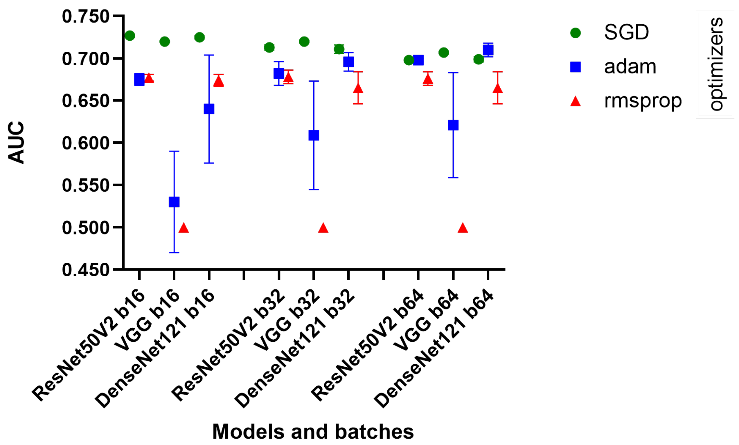
The first phase (Figure 1) of our process was the high-level quick tests, created using a very small amount of MIMIC-CXR data (training: 8000, validation: 1500, testing: 2500). The optimization experimented with different batch sizes of 16, 32, and 64 and different optimizers, namely Adam, Stochastic Gradient Descent (SGD), and RMSprop,

Table 3. Models’ performance on high-level quick tests.

Network	Trainable Param.	Batch	Optimizer	AUC
ResNet50V2	23.5M	16	SGD	0.727 ± 0.005
DenseNet121	6.9M	16	SGD	0.726 ± 0.002
VGG16	134.3M	32	SGD	0.723 ± 0.001
VGG16	134.3M	16	SGD	0.720 ± 0.001
ResNet50V2	23.5M	32	SGD	0.713 ± 0.003
DenseNet121	6.9M	32	SGD	0.711 ± 0.005
DenseNet121	6.9M	64	Adam	0.710 ± 0.008
ResNet50V2	23.5M	64	Adam	0.709 ± 0.010
VGG16	134.3M	64	SGD	0.707 ± 0.001
DenseNet121	6.9M	64	SGD	0.699 ± 0.003
ResNet50V2	23.5M	64	SGD	0.698 ± 0.002
DenseNet121	6.9M	32	Adam	0.696 ± 0.011
DenseNet121	6.9M	64	RMSprop	0.688 ± 0.024
ResNet50V2	23.5M	32	Adam	0.682 ± 0.014
ResNet50V2	23.5M	32	RMSprop	0.678 ± 0.008
ResNet50V2	23.5M	16	RMSprop	0.677 ± 0.004
ResNet50V2	23.5M	64	RMSprop	0.676 ± 0.008
ResNet50V2	23.5M	16	Adam	0.675 ± 0.007
DenseNet121	6.9M	16	RMSprop	0.674 ± 0.007
DenseNet121	6.9M	32	RMSprop	0.665 ± 0.019
DenseNet121	6.9M	16	Adam	0.640 ± 0.067
VGG16	134.3M	64	Adam	0.621 ± 0.062
VGG16	134.3M	32	Adam	0.609 ± 0.064
VGG16	134.3M	16	Adam	0.530 ± 0.060
VGG16	134.3M	64	RMSprop	0.500 ± 0.000
VGG16	134.3M	16	RMSprop	0.500 ± 0.000
VGG16	134.3M	32	RMSprop	0.500 ± 0.000

. These elements were key in fine-tuning the models, as batch size affects the generalization ability of the model, while optimizers play a key role in the speed and stability of the learning process. We used a fixed 10 epochs and 0.001 learning rate because the current aim of this phase was only to obtain a high-level analysis of the learning capabilities of the architectures.

We employed them in their most widely used basic configurations. We used the default configuration of optimizers; in the case of Adam, we used ${\beta }_1=0.9$ and ${\beta }_2=0.999$, and for RMSprop and SGD, we used $momentum=0$.

DenseNet121, ResNet50V2, and VGG16 showed consistent performance across different batch sizes. Remarkably, the decrease in AUC was minimal as the batch size increased, suggesting that these models maintain their efficiency even when processing larger batches. We see in Figure 3 that the SGD optimizer was consistently better than the others.

The standard deviations were generally low, indicating consistent performance across different runs of the models. However, with the Adam optimizer, a significant increase in the standard deviation was observed, especially for VGG16, which may indicate a less stable performance in these configurations.

3.2. Phase 2

For the second phase, as shown in Figure 1, we used ResNet50V2 exclusively for further experimentation. This decision was based on a confluence of factors, including the computational efficiency and simplicity of the model. Transfer learning, the cornerstone of our methodological framework, involves training a model on a large dataset and then adapting it to another, often smaller, dataset. This approach is particularly beneficial in medical imaging, where large annotated datasets are rare. Using the knowledge gained from one task, transfer learning improves the efficiency and generalization of learning on another task. In our study, we first trained ResNet50V2 on the entire MIMIC-CXR dataset, which provided a wide range of chest radiograph images. Learning from this dataset enables the base model to create a new promising model on Chest X-ray14. In this phase, we used 198,628 MIMIC-CXR images for training and 49,657 for validation. We trained for 50 epochs and chose the best checkpoint, according to the validation AUC.

3.3. Phase 3

In the third phase, as shown in Figure 1, we used ResNet50V2 without the top block and transferred the weights from Phase 2. It was used as a starting point in our Hyperband algorithm. In this phase of our deep learning model development, we focused on hyperparameter optimization to improve the performance of the model on our specific task. Hyperparameter optimization is crucial, as it involves tuning the model settings that are not learned from the data; however, these can significantly impact the learning process and the accuracy of the final model.

We identified several key hyperparameters for optimization: loss functions, optimizer settings, and learning rates. The choice of the loss function is particularly critical in defining how the model interprets the difference between the predicted and actual values during training. For our model, we considered two types of loss function: binary cross entropy (BCE) and sigmoid focal loss (SFL). SFL comes with additional parameters, namely alpha and gamma, that require fine-tuning. The optimizer chosen for this phase was stochastic gradient descent (SGD). We also optimized the momentum parameter, which is known for its effectiveness in navigating the parameter space; the momentum term helps accelerate the optimizer in the right direction.

The learning rate is one of the most important hyperparameters in neural network training. The aim is to determine the step size at each iteration while moving toward the minimum of the loss function. We experimented with various learning rates of 0.1, 0.01, 0.001, and 0.0001 to identify the optimal rate for our model.

After these settings, which affect the training process, we needed to build a new top block for ResNet50V2. The only mandatory layer was the last; we had to use a Dense Layer with 14 units and a sigmoid function for the activation. Nevertheless, we had the freedom to develop a new top between the end of the convolution part and this layer. The following table summarizes the hyperparameters (

Table 4. Hyperparameter optimization settings.

Hyperparameters	Range	${\mathit{Hyperopt}}_1$	${\mathit{Hyperopt}}_2$	${\mathit{Hyperopt}}_3$
Froze until	block2, block3, block4, block5	none	block 5	block3
Additional Block 1 Dense	none, 64, 128, 512	128	512	128
Additional Block 1 Dropout	0.0–0.8	0.4	0.4	0.4
Additional Block 2 Dense	none, 64, 128, 512	64	128	none
Additional Block 2 Dropout	0.0–0.8	0.5	0
Loss function	BCE, SFL	SFL (0.25, 2.0)	BCE	BCE
Optimizer	SGD (momentum: wo, 0.5, 0.9, 0.99)	0.9	0.9	0.5
Learning rate	0.1, 0.01, 0.001, 0.0001	0.1	0.01	0.01
Total parameters		23,836,173	24,681,229	23,828,749
Trainable parameters		23,790,733	1,116,429	22,337,293
Non-trainable parameters		45,440	23,564,800	1,491,456

) and their respective ranges or values that we explored in our optimization process. The first and second columns show the parameters and the ranges involved in hyperparameter optimization. $Hyperop{t}_1$, $Hyperop{t}_2$, and $Hyperop{t}_3$ showed some promising configurations of the process. These were retrained for the whole dataset in Phase 4. The Froze until parameter denotes how many blocks of ResNet50V2 were frozen. Dense 1,2 (the number means the units, and it uses the ReLU activation function) and Dropout 1,2 (the number means the dropout rate) denote the extra layers added for the classification part of the model. The loss, optimizer, and learning rate had their own ranges. In this phase, we used five-fold cross validation with only 0.2 of the Chest X-ray14 images, which was trained on 13,843 images and validated on 3461 images. We optimized over 15 epochs with a patience of five for the early stop on Hyperband.

3.4. Phase 4

In the last phase, we trained the optimized network on the whole Chest X-ray14 dataset. We used five-fold cross validation, with 69,219 training images and 17,305 validation images. We ran all the training for 30 epochs and chose the best model using the validation algorithm. All the model configurations presented in

Table 5. Evaluation of different approaches on ChestX-ray14: individual and mean AUC scores across 14 conditions.

	Imagenet Transfer 1	MIMIC-CXR Transfer 1	${\mathit{Hyperopt}}_1$	${\mathit{Hyperopt}}_2$	${\mathit{Hyperopt}}_3$
Atelectasis	0.7632 ± 0.0115	0.8207 ± 0.0143	0.7604 ± 0.0076	0.8063 ± 0.0078	0.8287 ± 0.0023
Cardiomegaly	0.6781 ± 0.0396	0.7162 ± 0.0190	0.8761 ± 0.0031	0.8798 ± 0.0061	0.8914 ± 0.0024
Consolidation	0.7943 ± 0.0197	0.8200 ± 0.0161	0.7383 ± 0.0148	0.7920 ± 0.0011	0.8094 ± 0.0041
Edema	0.7829 ± 0.0220	0.8280 ± 0.0234	0.8340 ± 0.0072	0.8835 ± 0.0098	0.8995 ± 0.0044
Effusion	0.8725 ± 0.0037	0.9227 ± 0.0101	0.8229 ± 0.0053	0.8746 ± 0.0077	0.8931 ± 0.0002
Emphysema	0.7239 ± 0.0092	0.7919 ± 0.0290	0.8658 ± 0.0085	0.8577 ± 0.0079	0.8847 ± 0.0033
Fibrosis	0.5977 ± 0.0183	0.7243 ± 0.0307	0.8039 ± 0.0080	0.7871 ± 0.0161	0.8086 ± 0.0027
Hernia	0.5774 ± 0.0409	0.6709 ± 0.0664	0.7571 ± 0.0991	0.8338 ± 0.0542	0.8130 ± 0.0378
Infiltration	0.6528 ± 0.0118	0.6968 ± 0.0079	0.6968 ± 0.0039	0.6803 ± 0.0162	0.7047 ± 0.0023
Mass	0.7215 ± 0.0130	0.7704 ± 0.0181	0.7836 ± 0.0113	0.8258 ± 0.0210	0.8518 ± 0.0020
Nodule	0.6564 ± 0.0161	0.7232 ± 0.0155	0.7207 ± 0.0095	0.7356 ± 0.0174	0.7588 ± 0.0025
Pleural Thickening	0.7129 ± 0.0336	0.7925 ± 0.0038	0.7585 ± 0.0121	0.7840 ± 0.0179	0.8121 ± 0.0025
Pneumonia	0.7010 ± 0.0151	0.8027 ± 0.0227	0.7094 ± 0.0060	0.7156 ± 0.0138	0.7304 ± 0.0072
Pneumothorax	0.7478 ± 0.0143	0.8657 ± 0.0079	0.8512 ± 0.0073	0.8392 ± 0.0138	0.8646 ± 0.0012
Mean	0.7130 ± 0.0020	0.7819 ± 0.0047	0.7842 ± 0.0007	0.8068 ± 0.0027	0.8250 ± 0.0023

¹ Stock ResNet50V2 with one Dense FC layer.

were evaluated on the official Chest X-ray14 testing set, which contains 25,596 images. We include some other models used in this phase to show the evolution in the improvement (Table 5). The ImageNet transfer column contains the best set from Table 3, which was run on the full Chest X-ray14 dataset with only ImageNet weights; we only changed the last layer to fit the Chest X-ray14 data. The MIMIC-CXR transfer column shows the pre-learned weights from Phase 2, with the configuration inherited from Phase 1. We only changed the last Dense layer to the correct number of labels. $Hyperop{t}_1$, $Hyperop{t}_2$, and $Hyperop{t}_3$ show these configurations run on the official split of Chest X-ray14.

3.5. Visual Representation

In this section, we present a visual interpretation of the learned features, using the Gradient-weighted Class Activation Mapping technique (Grad-CAM) [33]. Grad-CAM offers a technique to produce “visual explanations” for decisions from a broad array of CNN-based models, enhancing their transparency and interpretability. Grad-CAM utilizes the gradients of any target concept (e.g., ‘Effusion’ in the current context) flowing into the final convolutional layer to generate a coarse localization map. This map highlights the crucial regions in the image for predicting the concept [33]. Unlike prior methods, Grad-CAM can be applied to various CNN architectures without the need for re-training or architectural modifications.

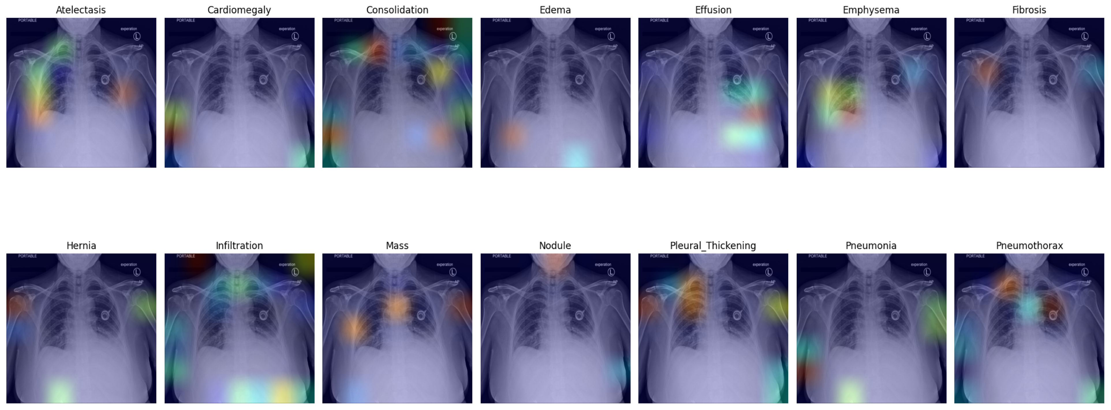
Figure 4 presents the default classifier head. In the first picture in the first row, atelectasis was mistaken due to overlapping rib arches. Since the left hemidiaphragm was obscured by the enlarged cardiac shadow, effusion in the fifth image in the first row is marked below the expected level of the diaphragm (blue). In the sixth image in the first row, emphysema was suggested, probably due to the significant difference in the overall density of the lung bases. In the third picture in the second row, the enlarged aortic knob was mistaken for a mass. In the seventh picture in the second row, pneumothorax was suggested in the right apex. This area is often difficult to assess for junior radiologists; as the bronchovascular pattern is faint, it can raise a false suspicion of pneumothorax.

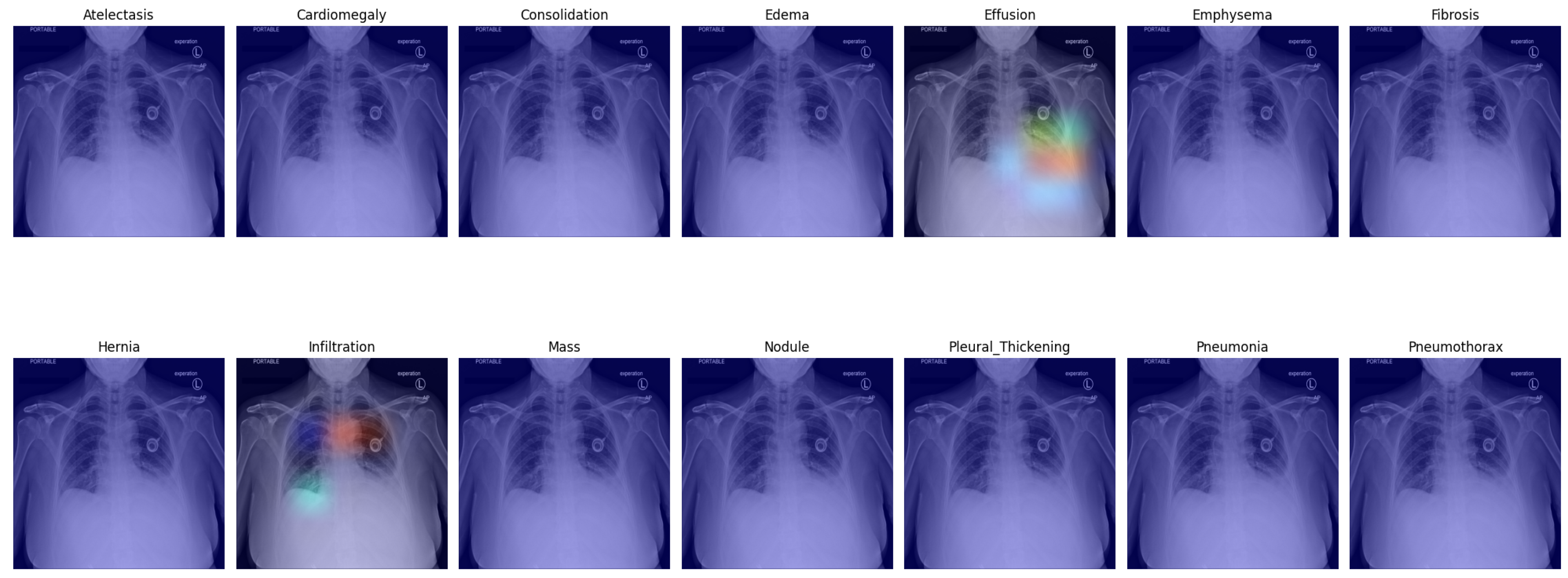
In Figure 5, we present a visual representation of our proposed enhanced model wherein the pleural effusion is marked in the fifth image in the first row, confirmed by a radiologist. In the second image in the second row, however, infiltration is falsely suggested, and the aortic knob was marked instead (red). Infiltration is less likely but probable in the right lower lung area. Infiltration is also likely as an underlying factor for the effusion on the left side; this was not suggested by the algorithm. Cardiomegaly was also not suggested, although it can be visually confirmed.

4. Conclusions

As presented, our proposed method shows a promising AUC ratio that outperforms many competing models in this research area. Remarkably, only two models achieved better AUC ratios than ours (

Table 6. Comparison of our results with various studies.

	Wang et al. [12]	Yao et al. [39]	Shen et al. [40]	Tang et al. [13]	Guan et al. [41]	Yan et al. [34] 1	Baltruschat et al. [35] 2	Kufel et al. [36] 3	Ours
Backbone	R50					R-50			R50
Atelectasis	0.700	0.733	0.766	0.765	0.792	0.792	0.763	0.817	0.8287
Cardiomegaly	0.810	0.856	0.801	0.887	0.879	0.881	0.875	0.911	0.8914
Consolidation	0.703	0.711	0.787	0.728	0.758	0.760	0.749	0.815	0.8094
Edema	0.805	0.806	0.820	0.848	0.850	0.848	0.846	0.908	0.8995
Effusion	0.759	0.806	0.797	0.819	0.824	0.842	0.822	0.879	0.8931
Emphysema	0.833	0.842	0.773	0.906	0.909	0.942	0.895	0.935	0.8847
Fibrosis	0.786	0.743	0.765	0.818	0.832	0.833	0.816	0.824	0.8086
Hernia	0.872	0.755	0.748	0.875	0.906	0.934	0.937	0.890	0.8130
Infiltration	0.661	0.673	0.751	0.689	0.694	0.710	0.694	0.716	0.7047
Mass	0.693	0.718	0.760	0.814	0.831	0.847	0.820	0.853	0.8518
Nodule	0.669	0.777	0.741	0.755	0.766	0.811	0.747	0.711	0.7588
Pleural Thickening	0.684	0.724	0.759	0.765	0.778	0.808	0.763	0.812	0.8121
Pneumonia	0.658	0.684	0.778	0.729	0.726	0.740	0.714	0.769	0.7304
Pneumothorax	0.799	0.805	0.800	0.850	0.858	0.876	0.840	0.898	0.8646
Mean	0.745	0.760	0.775	0.803	0.814	0.830	0.806	0.838	0.8250

¹ They use a bounding box of interest region. ² They use additional non-image features. ³ They use a non-official data split.

); however, their methodologies differ significantly from our approach. Yan et al. [34] used bounding boxes to focus on regions of interest (ROIs), which undoubtedly aids the learning process. However, our study deliberately focuses on minimizing human intervention. This approach is particularly important for large datasets, where manual annotation of ROIs is not possible due to the significant time and expertise required from already overloaded radiologists. Baltruschat et al. [35] used additional non-image features. They added the patient’s gender and age as a feature into a classifier that significantly improved lesions that depend on gender or age. Furthermore, one better result came from a study published by Kufel et al. [36] on 22 September 2023, which shows a remarkably high AUC; it is important to note that their results are based on custom data splitting. This unique data management makes comparison impossible for those who use the official one. The difference in data processing methods underscores the importance of standardizing research protocols to ensure fair and meaningful comparisons between studies. Our study provides an excellent base for future research in the field. One possible path is to address and overcome hardware limitations. This opens the way for experimentation with more computationally intensive models, such as ResNetV2 101 and 152 or creating higher hyperspace for the examinations. In addition, it opens another segment of the research to develop hyper-optimal ensemble methods that add the strengths of different network architectures. In summary, our research contributes to the current understanding of and methods used in medical image analysis and sets the stage for innovative future studies that may further push the boundaries of what is achievable in this rapidly evolving field. For future research, we want to use this technique for COVID CT images, in contrast to Chen et al. [37], and the long-term plan is to use this method in brain signal research, based on Zang et al. [38]. We think that recreating the classifier parts of well-known CNNs will open the door to several unexplored research fields.