Optimizing Cross-Dock Terminal Location Selection: A Multi-Step Approach Based on CI-DEA–IDOCRIW–MABAC for Enhanced Supply Chain Efficiency—A Case Study

Abstract

Thedistribution of products stands out as one of the pivotal activities for logistics companies in recent years, particularly in the aftermath of the COVID-19 pandemic and other geopolitical events. Intense competition compels companies to efficiently execute their logistical processes, with cross-docking emerging as a frequently applied solution. However, the location of cross-dock terminals in urban areas remains a problem insufficiently addressed in the literature, with a dearth of studies and models tackling this issue. This paper introduces a novel and innovative model for locating cross-dock terminals based on the CI-DEA–IDOCRIW–MABAC (Composite Indicators–Data Envelopment Analysis-Integrated Determination of Objective Criteria Weights–Multi-Attributive Border Approximation Area Comparison) methods. In the process of defining input indicators, the following three sources were utilized: relevant literature, practical insights from logistics experts, and the knowledge and experience of the authors. Eight inputs and three outputs were considered (the number of users in the observed channel; the area served by the channel; the average distance a vehicle travels in one delivery; the required number of vehicles; labor availability; competition; construction, and expansion possibilities; proximity to the main infrastructure and traffic facilities; the average number of deliveries; average delivered quantity; and service level). The model underwent testing in a case study analyzing nine distribution channels (areas within the observed urban zone). The results indicated that alternative A4 (in the southwest area) ranked the highest since it was the best-ranked in accordance with the most important criteria, suggesting that the terminal is best located in the southwest zone. The accuracy of the results was confirmed by company management. By developing a completely new model and addressing the identified gap in the literature, this paper provides unequivocal scientific contributions.

1. Introduction

Distribution process planning and execution is a key aspect of logistics. Among various strategies, cross-docking has gained popularity alongside direct delivery and storage-based approaches [1]. Direct delivery entails sending products directly from the manufacturer to the end customers, allowing the delivery company complete control over the process. This approach enhances customer relationship management, reduces delivery times, and cuts costs associated with bypassing storage facilities. However, a drawback of direct delivery is the underutilization of cargo space due to the frequent delivery of smaller product quantities. This results in increased transportation costs and longer delivery times. In response to these challenges, distribution strategies involving storage and cross-docking have emerged.

A storage-based strategy contributes to warehouse activities, especially order consolidation, optimizing transport vehicle capacity, and reducing transportation costs. Various warehouse systems and distribution centers facilitate the storage process [2]. This strategy also offers flexibility in responding to demand changes through inventory storage and management activities. Despite the advantages, implementing storage activities incurs additional costs. It is crucial to note that this strategy aims to ship goods when the transport vehicle’s cargo space is maximally filled to minimize transportation costs.

To address issues related to traditional warehousing, inventory ownership, and transportation costs, the cross-docking strategy comes into play. Cross-docking involves consolidating and shipping goods without storage or with limited temporary storage if necessary [3]. In a cross-dock terminal, incoming shipments are quickly unloaded, consolidated, and loaded onto outgoing transport vehicles on the same day. If temporary storage is required, it typically lasts no more than 24 h, according to several authors. Implementing the cross-dock strategy enhances transportation efficiency and cost-effectiveness without the overheads associated with traditional warehousing systems. Also, cross-docking reduces lead times and can impact improving customer order delivery time [4,5].

However, it is essential to recognize that the cross-dock strategy is not a universal solution. It requires significant quantities of goods with a high turnover rate, a sophisticated information system, and precision in coordinating incoming and outgoing transport vehicles. Operators and users may encounter various strategic, tactical, and operational challenges during cross-dock strategy implementation. In addition to cost-effectiveness, one of the most important challenges of the cross-dock strategy is terminal location. Terminal location directly affects distribution costs on the one hand, while on the other hand, it influences the level of service quality provided.

The subject and objective of this paper entail the development of an innovative model to address the challenges associated with the location of cross-docking terminals. This model is based on the implementation of the CI-DEA–IDOCRIW–MABAC methodology. Firstly, the CI-DEA method was applied in order to reduce the initial number of inputs/outputs based on the correlation. In the next phase, the IDOCRIW method was applied to determine criteria weights, while in the last phase, the MABAC method was applied in order to rank the alternatives (in this case, potential cross-docking locations). The developed methodology was employed to address a case study encompassing a large region. The CI-DEA method is based on the principles of PCA-DEA [6], where the main objective is to reduce the number of inputs and outputs used for the evaluation of DMUs by taking into account the correlation between inputs/outputs and, hence, reducing their number. The reason for implementing this method in the paper is reflected by the fact that the implementation of the CI-DEA model results in an unambiguous and easy interpretation of the obtained results. Also, another reason for its implementation is the fact that, based on the simulation results [7], it was determined that this method assessed the DMU efficiency better than the standard DEA, and the results seemed to be more reliable. The IDOCRIW method was applied since the goal of this paper was to determine criteria weights objectively. This approach combines the weights obtained from entropy and criterion impact loss (CILOS) methods in order to obtain the aggregate criteria weights. By applying both of the previously mentioned methods through the IDOCRIW method, the drawbacks associated with one methodology are compensated by the strengths exhibited in the alternative approach [8]. Finally, the MABAC method was applied for ranking because this method represents a useful and reliable tool for rational decision making and provides consistent (stable) solutions [9].

The structure of this paper is as follows: Section 2 offers an in-depth exploration of the problem, accompanied by a relevant literature review. In this section, aside from defining the concept, the significance and characteristics of implementing the cross-docking strategy are expounded upon. Section 3 introduces a multi-stage model developed for determining the location of cross-docking terminals in the distribution network. A comprehensive presentation of the case study considered in this paper is provided in Section 4, inclusive of the results. Section 5 delves into a more detailed analysis of sensitivity, as well as its theoretical and managerial implications and contributions. Finally, concluding remarks and future research directions are articulated in Section 6.

2. Problem Description and Literature Review

2.1. Cross-Dock Definition

Cross-docking represents a distribution strategy that has become increasingly prevalent over the last few decades. In the business realm, the significance of cross-docking began to emerge in the second half of the 1980s, notably with its implementation in the supply chain of retailers such as Walmart, resulting in significant savings and cost reductions. The example of Walmart has indeed generated substantial interest among researchers in the field of the cross-dock strategy [10].

Defining cross-docking as a concept sparks significant debate, leading to a myriad of diverse definitions that highlight specific characteristics. However, at its core, these definitions all converge on the idea that cross-docking is a logistics strategy aiming to minimize inventory and transportation costs by consolidating the various flows of goods with different origins at a single terminal. Below is an overview of this dispersion in definitions, presenting a general definition and one from the Material Handling Industry of America.

The general definition of the cross-dock strategy is as follows [11]:

“Cross-dock involves receiving products or materials from suppliers or manufacturers for multiple end destinations and consolidating the received products with products from other suppliers for a common destination, based on certain criteria”.

On the other hand, the definition from the Material Handling Industry of America is the following [11]:

“Cross-dock involves the process of moving goods from the receiving to the shipping dock without storage between the receiving and shipping docks”.

Within these two definitions, one can discern an aspect of diversity as well as simultaneous similarity. Specifically, the emphasis in the first “general” definition is on consolidation to achieve greater economic efficiency by minimizing transportation costs. In contrast, the second definition focuses on dispersion regarding the movement of goods. However, fundamentally, the goal of the definitions is the same. The fundamental processes executed within the cross-dock terminal are illustrated in Figure 1.

2.2. Cross-Dock Implementation

The adoption of the cross-docking concept has become increasingly prevalent, driven by a heightened awareness of its benefits and popularity in recent decades. However, it is crucial to acknowledge that the cross-docking concept may not always represent the optimal strategy. Some authors argue that the cross-docking strategy is most suitable for goods characterized by high, predictable demand and specific quantity requirements, especially those with a diminishing value aspect [12,13].

Furthermore, certain authors argue that the application of the cross-dock concept is optimal when specific factors are satisfied. There are variations in the consideration of these factors among different authors. The first crucial factor is the level of demand for the product. If there are fluctuations in demand over time, the cross-dock strategy is deemed suboptimal unless implemented with an appropriate planning system. Therefore, the cross-dock strategy is deemed optimal for products with a consistent demand. The second factor is the cost of stockouts [11].

In addition to the factors previously mentioned, there are other variables that can impact the suitability of implementing the cross-dock concept. Some of these factors include the following [3,4,10,11]:

• The distance between suppliers and customers;
• The value and lifecycle of the product;
• The required quantity of products;
• Timeliness of delivery, etc.

2.3. Cross-Dock Characteristics

The performance of cross-dock terminals can be assessed using various performance indicators. Some of the performance indicators that need to be monitored in a cross-dock terminal are described below [13].

• Inventory Level—since one of the primary motivations for implementing the cross-dock strategy is to reduce inventory levels, it is essential to have indicators related to monitoring the overall or maximum quantity of stocks stored in the terminal at any given time or moment.
• Congestion—the drive to minimize the overall distance traveled within the cross-dock terminal can lead to the clustering of loading and unloading activities in a very confined space, potentially causing congestion and significantly reducing the productivity of a cross-dock terminal.
• Total Dwell Time of Goods—given that the primary objective of a cross-dock terminal is to minimize inventory levels and, consequently, the dwell time of goods, it is essential to monitor the overall dwell time of goods as a crucial performance indicator.
• Time for Loading and Handling Operations—in order to minimize the overall dwell time of goods and, concurrently, inventory levels, it is necessary to define the time required for the loading and unloading of incoming and outgoing vehicles and ensure adherence to the defined time frames.
• Number of Material Handling Operations—Depending on the design and purpose of the cross-dock terminal, goods within the terminal may undergo handling once, twice, or more, depending on the activities involved. Each material handling operation requires the engagement of resources and, thus, introduces additional cost burdens. Therefore, the average number of handling operations for a specific type of goods represents a potential performance indicator, etc.

2.4. Location Problem

In the development of a cross-dock terminal, distinct phases are navigated, each requiring decisions at the strategic, tactical, and operational levels. Consequently, challenges arise at different decision-making tiers, which are aligned with the stages in the evolution of a cross-dock terminal. The initial decisions revolve around the strategic planning phase of the cross-dock strategy and pertain to strategic elements such as the location and layout of the cross-dock terminal. Following this, at the tactical level, decisions are made regarding the execution of internal transport, the selection of loading and handling equipment, operational methodologies, and capacity planning. Subsequently, operational-level decisions fall under the responsibility of the cross-dock terminal operator and involve aspects like vehicle routing, temporary storage, arrival, and departure schedules, preferences for specific transportation modes, and the allocation of loading docks to vehicles [11,14].

The extensive range of decision-making issues mentioned, organized across a timeline from long-term strategic to short-term operational problems, can be presented as follows [11,12,14,15,16,17]:

• Location problem, i.e., the decision-making process for the location of the cross-dock terminal while adhering to the existing distribution network structure;
• Scheduling incoming and outgoing vehicles;
• The layout of the cross-dock terminal;
• The allocation of destinations, i.e., defining positions on the loading dock that specific vehicles occupy based on their origin or final destination;
• Scheduling the loading and unloading operations of vehicles, i.e., defining the sequences in which arriving vehicles are serviced;
• The organization of internal transport within the cross-dock terminal.

The cross-dock location problem has been recognized in the literature, although the proposed models are mainly based on the implementation of heuristics and metaheuristics. For instance, Ref. [18] proposes a model for selecting the cross-dock location while simultaneously determining a fleet of vehicles used to transport goods from suppliers to the end users (assembly parts). In order to solve this NP-hard problem, a biogeography-based optimization (BBO) algorithm was used. The authors compared this approach with particle swarm optimization (PSO), and the results showed that the BBO performs much better in terms of total network costs and computational time. Two Lagrangian relaxation algorithms were proposed in [19] to define a reliable cross-dock network even in situations of disruptions. Meidute-Kavaliauskiene et al. [5] focused on several problems regarding the cross-docks. Namely, the authors proposed an algorithm based on the implementation of the non-dominated sorting genetic algorithm-II (NSGA-II) and multi-objective particle swarm optimization (MOPSO) for targeting the following three issues: cost optimization, scheduling incoming and outgoing vehicles, and green supply chains (SC) consisting of several cross-docks. Similarly, Rostami et al. [20] proposed a model for addressing the optimization of incoming and outgoing vehicle schedules in order to minimize the total operation time within SC. The observed SC consists of suppliers, cross-docks, and factories. Several algorithms were then used by the authors in order to solve this NP-hard problem. Rahbari et al. [21] proposed two robust bi-objective models taking into account the traveling time (for outgoing vehicles) and freshness-life of perishable products in order to solve the vehicle routing problem. Similarly, Shahabi-Shahmiri et al. [22] proposed a model for solving the routing and scheduling problems of perishable products that are distributed via a cross-dock. The aim of the model was to minimize distribution costs and shorten the distribution time while maximizing the capacity utilization of the cross-docking network. A multi-objective optimization model for solving the routing problem and the cross-dock selection problem by applying Pareto-based algorithms was proposed by [23]. A mathematical model for truck scheduling taking into account a multidoor cross-dock was proposed by Taghizadeh et al. [24]. Soleimaninanadegany et al. [25] developed a model based on a genetic algorithm (GA) for product allocation to the warehouse and cross-dock. Cross-docks can also have an impact on the efficiency of the company. With this in mind, a framework for designing cross-docks in order to improve the overall efficiency of the distribution process was developed in [26].

On the other hand, after conducting the literature review, it was concluded that only a few papers solved the described problem using MCDM (Multi-Criteria Decision-Making) methods. Deng and Qu [16] focused on determining the cross-dock center location by applying Interval Multi-Granularity Multi-criteria Group Decision-Making. Mousavi et al. [15] developed a hybrid fuzzy possibilistic–stochastic programming solution approach for solving the two most common and crucial problems, i.e., determining locations for multiple cross-docks and scheduling incoming and outgoing vehicles. As already explained, goods are stored for only a short period in cross-docks. In these situations, it is essential to determine the location of every unit load. This problem was addressed by [4] in order to determine the optimal storage location for the unit load with the aim of minimizing the travel distance of forklifts when manipulating these units. Since a certain dose of uncertainty is present in selecting a location for a cross-dock, the authors in [17] determined that conventional models are not sufficient. Therefore, they developed a novel model based on Interval-Valued Intuitionistic Fuzzy (IVIF) sets to tackle this uncertainty. The aforementioned models do not include methods for eliminating subjectivity (like CI-DEA in this paper), and this represents their main limitation.

3. Methodology

To tackle the described problem, a methodology based on the implementation of the CI-DEA–IDOCRIW–MABAC method was proposed in this paper. The proposed approach consists of several phases (Figure 2). In the first phase, a literature review and interviews with experts from the observed company were conducted to determine the inputs and outputs that would be taken into account in this paper. Based on the results of this phase, in the second step, the CI-DEA method was applied, firstly to reduce the number of observed inputs/outputs since only nine DMUs (distribution channels) were analyzed and, secondly, the implementation of the DEA method resulted in very poor discriminatory power (since all DMUs were efficient). In the next phase, only efficient DMUs were taken into account. During this phase, again, based on a literature review and interviews with experts from the observed company, criteria for the evaluation of alternatives were defined. The IDOCRIW method was applied in this phase to obtain the criteria weights. These values were then used in the final phase using the MABAC method to rank the alternatives (for potential cross-dock locations).

3.1. CI-DEA Method

CI-DEA was proposed in [7] to reduce the number of observed input/output indicators, which is especially significant in a situation when there is a large number of inputs/outputs and a smaller number of DMUs. This reduction is achieved by taking into account the correlation that exists among indicators. The input-oriented CI-DEA model can be defined using Equations (1)–(4) as follows [7].

$$\underset{V_o{U}_o{V}_{o,\mathit{CI}}{U}_{o,\mathit{CI}}}{\max }{U}_o^T{Y}_o+U_{o,CI}^T{Y}_{o,CI}$$

(1)

s.t.

$$V_o^T{X}_o+V_{o,CI}^T{X}_{o,CI}=1$$

(2)

$$V_o^T{X}_j+V_{o,CI}^T{X}_{j,CI}-U_o^T{Y}_j-U_{o,CI}^T{Y}_{j,CI}\ge 0$$

(3)

$$V_o,U_o,V_{o,CI},U_{o,CI}\ge 0$$

(4)

where $X_o$ represents vector of m inputs for the o-th DMU; $Y_o$ represents vector of s outputs for the o-th DMU; $V_o$ represents vector for input multipliers; $U_o$ represents the vector for output multipliers; $X_j$ and $Y_j$ represent input and output vectors for the remaining n DMUs (j = 1, 2, …, n), respectively; $X_{o,CI}$ and $Y_{o,CI}$ are the input and output vectors of CIs for o-th DMU; and $V_{o,CI}$ and $U_{o,CI}$ represent vectors of multipliers related to $X_{o,CI}$ and $Y_{o,CI}$, respectively.

3.2. IDOCRIW Method

The implementation steps of the IDOCRIW method are as follows [27].

Step 1. Formation of the initial decision matrix.

Step 2. Normalization of the initial decision-making matrix using Equation (5).

$${\tilde{x}}_{ij}=\frac{{\mathrm{x}}_{ij}}{\sum _{i=1}^n{\mathrm{x}}_{ij}}$$

(5)

Step 3. Calculating the entropy of every variable or criterion using Equation (6).

$$E_j=-\frac{1}{\mathrm{l}\mathrm{n}\left(n\right)}\sum _{i=1}^n{\tilde{x}}_{ij}\ln \left({\tilde{x}}_{ij}\right); j=1,2,\dots ,m;0\le E_j\le 1$$

(6)

Step 4. Determining every alternative’s uncertainty or degree of deviation by applying Equation (7).

$$d_j=1-E_j; j=1,2,\dots ,m$$

(7)

Step 5. The calculation of the weight for each alternative using Equation (8).

$$w_j=\frac{d_j}{\sum _{j=1}^m{d}_j}; j=1,2,\dots ,m$$

(8)

Step 6. Creating a square matrix where the maximum values of each column from the normalized matrix are selected to create this matrix by applying Equation (9).

$$a_j=\underset{i}{\max }{\tilde{x}}_{ij}=a_{kij}; i=1,2,\dots ,n; j=1,2,\dots ,m$$

(9)

where $a_{kij}$ is equal to the highest criterion value or the j-th column extracted from the sample or row k_i. To create a square matrix with m × m dimensions, the elements $a_{ij}$ are set equal to $a_{kij}$ and $a_{jj}$ is assigned the value of $a_j$. Consequently, the i-th row of the square matrix incorporates the elements from the k_i row of the normalized matrix, ensuring a matrix with consistent dimensions.

Step 7. Determining the lost impact matrix by applying Equation (10).

$$p_{ij}=\frac{a_{jj}-a_{ij}}{a_{jj}}; i,j=1,2,\dots ,m; p_{jj}=0$$

(10)

where $p_{jj}$ represents the loss of the relative effect of the criterion or j alternative if the i-th criterion is selected as the best solution.

Step 8. Determining the matrix of the weight system using Equation (11).

$$\mathrm{F}=\left[\begin{array}{c}\begin{array}{ccc}-{\displaystyle \sum _{i=1}^m}{p}_{i2}& p_{12}& \cdots p_{1m}\\ p_{21}& -{\displaystyle \sum _{i=1}^m}{p}_{i2}& \cdots p_{2m}\\ ⋮& ⋮& \ddots \end{array}\\ p_{m1} p_{m2} \cdots -{\displaystyle \sum _{i=1}^m}{p}_{im} \end{array}\right]$$

(11)

Step 9. Criteria weights are determined using the criterion impact loss method (CILOS). Assuming the weight of each criterion or variable is denoted as q_j, and these weights are derived using Equation (12).

$$F{q}^T=0$$

(12)

where q^T represents the linear vector of weights (q = [q¹, q², …, q^m]. When using the CILOS method to determine criteria weights, the following condition must be met: $\sum _{j=1}^m{q}_j=1$.

Step 10. Determining the criteria weights using the cumulative method (weights are obtained using the entropy and CILOS methods) by applying Equation (13).

$${\omega }_j=\frac{q_j{w}_j}{\sum _{j=1}^m{q}_j{w}_j}; j=1,2,\dots ,m$$

(13)

where ${\omega }_j$ represents the weight of the j-th criterion.

3.3. MABAC Method

When implementing the MABAC method, the following steps must be conducted [9,28].

Step 1. Define the initial decision-making matrix (X) with m alternatives and n criteria.

Step 2. Normalize the initial decision-making matrix (X) by applying Equation (14) for benefit criteria and (15) for cost criteria.

$$n_{ij}=\frac{x_{ij}-x_i^{-}}{x_i^{+}-x_i^{-}}$$

(14)

$$n_{ij}=\frac{x_{ij}-x_i^{+}}{x_i^{-}-x_i^{+}}$$

(15)

where x_ij, $x_i^{+}$ and $x_i^{+}$ represent the elements obtained from the initial decision-making matrix using Equations (16) and (17):

$$x_i^{+}=\mathrm{m}\mathrm{a}\mathrm{x}(x_1,x_2,\dots ,x_m)$$

(16)

$$x_i^{-}=\mathrm{m}\mathrm{i}\mathrm{n}(x_1,x_2,\dots ,x_m)$$

(17)

Step 3. In this step, the weighted decision-making matrix (V) is determined by applying Equation (18).

$$v_{ij}=w_i\times (n_{ij}+1)$$

(18)

Step 4. The border approximation area (BAA) matrix (G) is determined by applying Equation (19).

$$g_i={(\prod _{j=1}^m{v}_{ij})}^{1/m}$$

(19)

Step 5. In order to form matrix Q, the calculation of the distance of the alternative from the BAA is conducted. The determination of the alternative’s proximity to the border approximation area (q_ij) involves computing the discrepancy between elements in the weighted matrix (V) and the value assigned to the border approximation area (G). In this context, g_i denotes the border approximation area associated with criterion C_i, while v_ij represents the weighted matrix of the elements (V).

Alternative A_i is subject to classification into the border approximation area (G), upper approximation area (G⁺), or lower approximation area ($G^{-}$) articulated as $Ai\in \{G\vee G^{+}\vee G^{-}\}$. The upper approximation area (G⁺) encapsulates the ideal alternative (A⁺), whereas the lower approximation area ($G^{-}$) comprises the anti-ideal alternative ($A^{-}$). The assignment of alternative A_i to the approximation area (G, G⁺, or $G^{-}$) can be performed using Equation (20).

$$Ai\in \left\{\begin{array}{c}{G}^{+} if q_{ij}>0\\ G if q_{ij}=0\\ G^{-} if q_{ij}<0\end{array}\right.$$

(20)

Step 6. In the final step, alternatives are ranked by calculating the values of the criterion functions for the alternatives using Equation (21).

$$S_i=\sum _{j=1}^n{q}_{ij},j=1,2,\dots ,n\hspace{1em}i=1,2,\dots ,m$$

(21)

4. Optimizing Cross-Dock Terminal Location Selection–Case Study

In the preceding sections of this paper, general forms of distribution strategies, along with their concept, types, characteristics, application, and implementation, as well as the challenges, performance metrics, advantages, and disadvantages of the cross-dock strategy, are presented. In this chapter, we delve into the issue of locating cross-dock terminals, recognizing it as a paramount challenge. The initial segment provides an overview of the observed system, with a specific focus on its operational framework, taking into account certain constraints and formulating the problem that necessitates a resolution. The subsequent segment addresses the procedural application of the methodology developed in this study, presenting and analyzing the obtained results.

4.1. Case Study Description

The observed company, among other activities, engages in providing distribution services for fast-moving consumer goods across a broader geographical area for various clients. The distribution system is anchored in a central distribution center, dispatching vehicles with various capacities and specifications to carry out a nationwide distribution. Following a comprehensive analysis, the company determined the need to implement a cross-dock terminal for a region covering approximately 4000 km². This company set out to identify the most optimal channel for introducing the cross-dock facility.

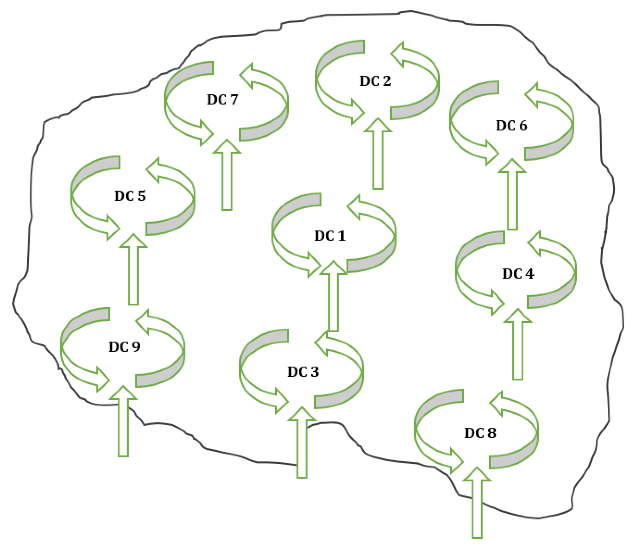
In order to tackle the issue, data spanning from 1 January 2022 to 1 January 2023 were employed. The observed timeframe was considered significant as it encompasses diverse variations in the demands attributed to seasonal patterns and other internal and external factors. The distribution within the examined area is categorized into nine primary distribution channels (DCs) (Figure 3).

• Distribution Channel 1–The Narrowest Central City Zone;
• Distribution Channel 2–Northern Part of the Area;
• Distribution Channel 3–Southern Part of the Area;
• Distribution Channel 4–Eastern Part of the Area;
• Distribution Channel 5–Western Part of the Area;
• Distribution Channel 6–Northeastern Part of the Area;
• Distribution Channel 7–Northwestern Part of the Area;
• Distribution Channel 8–Southeastern Part of the Area;
• Distribution Channel 9–Southwest Part of the Area.

All distribution channels are executed in the same manner. Vehicles, loaded with prepared orders, are dispatched from the main distribution center to specific locations.

In response to the company’s request to identify the most justified distribution channel for introducing a cross-dock facility, it was imperative to define the relevant parameters for evaluating the observed channels. To ensure the utmost reliability of the results, this study synergized data from the following three sources:

• Indicators utilized in the literature;
• Information and requirements provided by the company’s management;
• The prior knowledge and experience of the authors.

Through several iterations, a final set of 11 variables was determined by combining the following mentioned sources:

• The number of users in the observed channel (I1);
• The area served by the channel (I2);
• The average distance a vehicle travels in one delivery (I3);
• The required number of vehicles (I4);
• Labor availability (I5);
• Competition (I6);
• Construction and expansion possibilities (I7);
• Proximity to the main infrastructure and traffic facilities (I8);
• The average number of deliveries (O1);
• Average delivered quantity (O2);
• Service level (O3).

The number of users in the observed channel is a highly significant indicator as it serves as the catalyst for all logistics requirements. Therefore, it is positioned as the first in a series of 11 parameters. This indicator is frequently referenced in the literature [17,29,30], as well as in practical applications.

The area served by the channel provides essential information about the geographical locations of users. Among other factors, this parameter can impact the required number of vehicles and the distances covered.

The average distance denotes the total distance covered by a vehicle in one tour, expressed in kilometers. Unlike time, this metric offers more comprehensive insights into the “coverage” of the area and its associated costs.

Each of the observed channels has a specific fleet size. The required number of vehicles is defined as the minimum necessary to serve users in that area, representing one of the most commonly utilized parameters in the literature.

Labor availability is one of the specific parameters under scrutiny in this analysis. The shortage of labor in the logistics market of an observed country necessitates the inclusion of this variable. In each distribution channel, the number of available workers required for future cross-dock activities varies. It is crucial to note that this involves a larger geographical area, and workers are not available to commute between zones, given the traffic congestion and the necessary travel time.

Competition is an inevitable indicator when it comes to the implementation of logistics services. The execution of services by the planned cross-dock terminal can be significantly influenced by other providers offering similar services in the observed area.

The possibility of construction and potential expansion is crucial for logistics managers. This parameter is largely influenced by factors such as available land and costs.

The closeness to key infrastructure is pivotal for efficiency and the prompt execution of services. It affects both the inbound transport to the cross-dock and the outbound delivery to end-users. Locations within the observed channels exhibit substantial variations in this aspect.

The average number of deliveries is a crucial operational indicator that must not be disregarded in such decision-making processes. This parameter has been extensively utilized in the literature.

Similarly, the average quantity per delivery is a key traffic indicator, reflecting the volume of operations in a distribution channel. Unlike comparable financial metrics, it offers a wealth of information beneficial to the logistics system.

The final parameter is the level of service quality provided. In the literature, various indicators such as service level, OTIF (On-Time In-Full), delivery time, lead time, etc., are employed [31,32,33]. The observed company utilizes the metric of successfully fulfilled services expressed as a percentage.

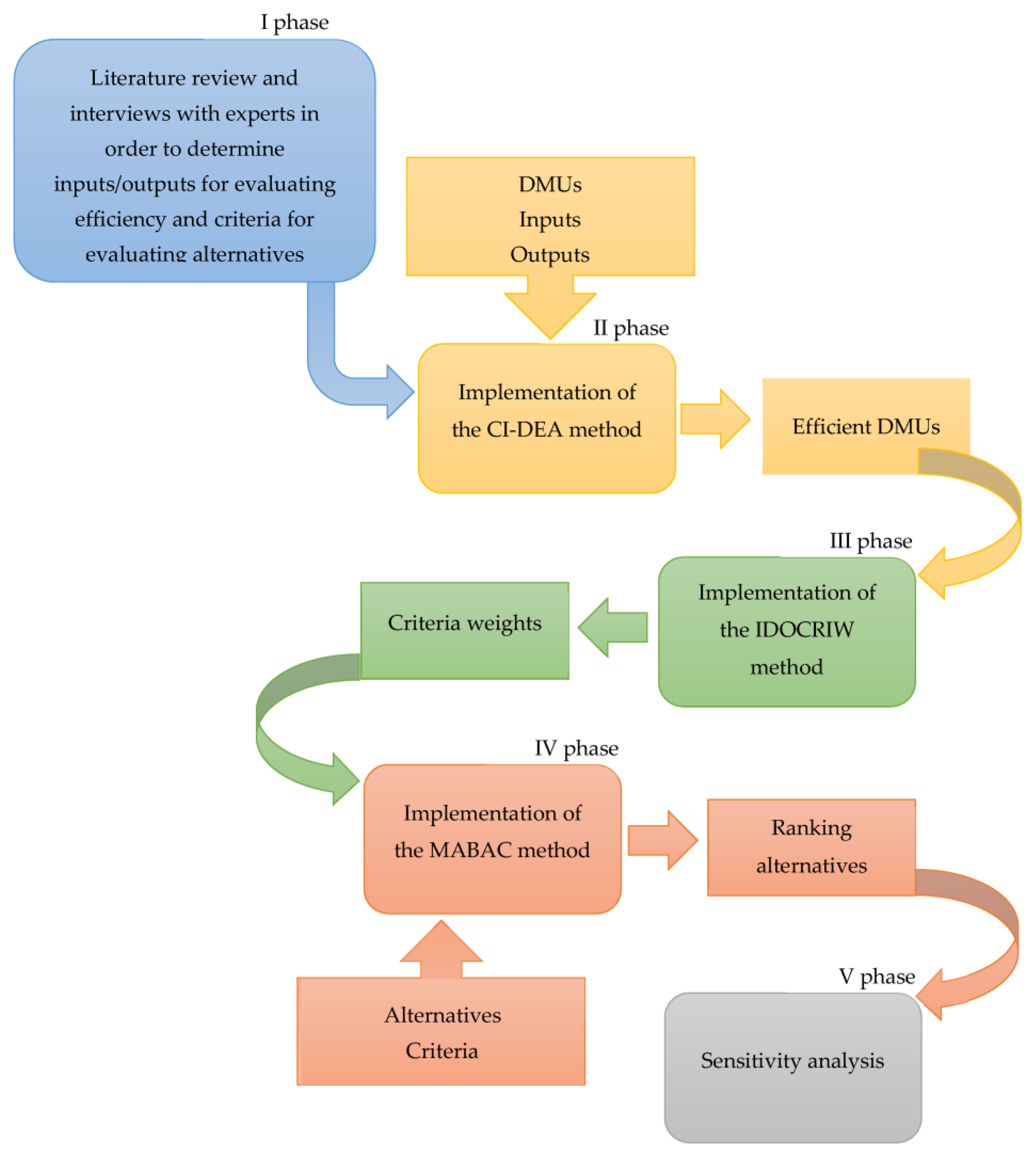
In the initial phase of evaluating the observed channels using the CI-DEA approach, the efficiency of these channels was appraised. The first 8 indicators were employed as input variables (the number of users in the observed channel (I1); the area served by the channel (I2); the average distance a vehicle travels in one delivery (I3); the required number of vehicles (I4); labor availability (I5); competition (I6); construction and expansion possibilities (I7); and proximity to the main infrastructure and traffic facilities (I8)), while 3 indicators were used as outputs (the average number of deliveries (O1); average delivered quantity (O2); and service level (O3)). The data used for this analysis are presented in

Table 1. Inputs and outputs of the CI-DEA model.

DMU	DC	I1	I2	I3	I4	I5	I6	I7	I8	O1	O2	O3
DMU1	City center	4123	55,106	84	25	7	3	10	9	6	1.80	0.93
DMU2	North	1749	37,468	129	20	8	10	8	4	8	2.32	0.94
DMU3	South	3418	48,036	178	19	3	6	5	4	11	3.24	0.98
DMU4	East	2772	64,365	148	23	7	5	6	6	10	3.95	0.99
DMU5	West	3885	38,246	126	12	6	6	7	7	7	2.86	0.96
DMU6	Northeast	1324	47,990	149	22	5	8	8	4	8	2.12	0.93
DMU7	Northwest	2120	54,569	173	24	5	9	9	3	5	2.35	0.99
DMU8	Southeast	2174	34,685	122	17	4	4	4	3	11	4.52	0.98
DMU9	Southwest	1286	25,176	164	19	5	3	3	2	13	3.02	0.99

.

4.2. Results

4.2.1. CI-DEA Results

In accordance with the methodology outlined in Chapter 3, the initial phase involved the application of the CI-DEA method. The utilization of the standard DEA approach did not provide satisfactory results. Namely, employing the standard DEA approach [34,35,36,37] resulted in an efficiency score of one for all nine distribution channels. Consequently, the CI-DEA approach was employed to overcome this limitation.

It is highly important to emphasize that the existence of correlation among variable dimensions (inputs and outputs) in the DEA method is not desirable. A high degree of interdependence can impact the discriminatory power of the model, prompting the often-recommended practice of retaining only one indicator from a set of correlated variables while excluding others from further analysis. In this regard, the novel CI approach recommends reducing the number of variables by constructing new (artificial) variables derived from the original data. This process allows decision makers to influence the significance of each original variable in the newly formed component.

In the initial phase, an independent correlation analysis of inputs and outputs was conducted. A correlation threshold of 0.5 or higher was employed to determine the relationship between variables and facilitate the creation of artificial components. Within the set of input components, two artificial components were generated, while two inputs were retained and utilized in their original form. The essential variables, such as the required number of vehicles and competition (inputs 4 and 6), were preserved in their original form. On the other hand, inputs 1, 3, and 8 (the number of users in the channel, the average distance in one delivery, and proximity to infrastructure) were combined to form the first artificial component, with weighting coefficients of 0.4, 0.3, and 0.3, respectively. Inputs 2, 5, and 7 (the area served, labor availability, and potential for construction and expansion) constituted the elements of the second artificial component and were each assigned an equal weight of 0.33. As a result, the total number of inputs was reduced from 8 to 4, significantly augmenting the model’s discriminatory power.

Within the output category, all three variables were employed to formulate a novel unified output indicator. In this context, the average number of daily deliveries, average delivered quantity, and service level were combined to form a new variable, with their respective significances in the new component being 0.4, 0.3, and 0.3.

Both the CCR and BCC models were utilized, but in further analysis, the results of the BCC model were considered. The ensuing results are reflective of the BCC input-oriented model (

Table 2. The efficiencies of the examined channels using both the standard DEA approach and the CI-DEA approach.

DMU	DMU Name	Standard DEA Efficiency Score	CI DEA Efficiecy Score
DMU1	City center	1	1
DMU2	North	1	0.92362
DMU3	South	1	0.891737
DMU4	East	1	0.752411
DMU5	West	1	1
DMU6	Northeast	1	0.912124
DMU7	Northwest	1	0.787446
DMU8	Southeast	1	1
DMU9	Southwest	1	1

). It is noteworthy that, when applying the CI approach, only 4 out of the 9 decision-making units (DMU) were deemed efficient, yielding an average efficiency of approximately 0.91. This underscores a markedly enhanced discriminatory power compared to the standard DEA approach. This improvement is a direct consequence of the reduction in the overall number of inputs and outputs, streamlined from 11 to 5.

The units found to be efficient in this phase are further scrutinized in subsequent analyses.

4.2.2. IDOCRIW Results

Following the application of the CI-DEA method and the identification of efficient units, the next step involved defining the criteria used for evaluating alternatives (potential locations for cross-dock terminals). The criteria employed in this study were established through a comprehensive literature review and interviews with experts from the company under consideration in this case study (

Table 3. Criteria used for potential location evaluation.

Criterion	Definition	References
Investment costs (C1)	Investment costs required to open a cross-dock terminal at a certain location (data provided by the company)	[30,38,39]
Cross-docking capacity (C2)	Cross-docking capacity in terms of inbound/outbound doors, temporary storage area, etc.	[17]
Proximity to the customers (C3)	Observed average delivery time	[17,29,30]
Competitiveness (C4)	The number of competing companies observed situated in close proximity to the location	[38]
Expansion possibility (C5)	The potential for expanding the cross-dock terminal at a specific location	[17,30]
Proximity to the infrastructure (C6)	Proximity to infrastructure (highways, roads, city) aimed at reducing the time required for the delivery of goods	[29,30,38,39]
Labor availability (C7)	Labor availability near the cross-dock terminal location (data provided by the company)	[29,38]
Impact on service level (C8)	The influence of constructing a cross-dock at a specific location at the service level (data obtained from the company)	[38]
Distribution costs (C9)	Distribution costs from the cross-dock terminal to end-users (estimated value provided by the company)	[17,38]

). It is crucial to emphasize that certain criteria were evaluated on a scale of 1–5 while others were evaluated using a scale of 1–10. The reason for this lies in the fact that certain values when considering these criteria, had to be divided into more intervals in order to improve the discriminatory power of the model. This approach was adopted to safeguard the confidentiality of the company’s data, which is the focal point of this case study. Given the involvement of six experts in the evaluation process, the average value of their assessments was used as a consolidated measure.

Following the establishment of criteria, the assessment of alternatives in accordance with all the criteria began, resulting in the formation of the initial decision matrix (

Table 4. Initial decision-making matrix.

Alternative/Criteria	C1	C2	C3	C4	C5	C6	C7	C8	C9
Type	min	max	min	min	max	max	max	max	min
City center (A1)	3	4	2	6	3	2	4	2	4
West (A2)	3	2	3	3	4	3	5	3	5
Southeast (A3)	5	5	4	4	7	7	7	4	4
Southwest (A4)	4	3	5	6	10	9	6	5	3

). This matrix serves as the input for the IDOCRIW method to determine the criteria weights.

Following the steps outlined in Section 3.2 and utilizing Equations (5)–(13), the criteria weights were derived (

Table 5. Criteria weights obtained after applying the IDOCRIW method.

Criterion	C1	C2	C3	C4	C5	C6	C7	C8	C9
Weights	0.0340	0.1266	0.0643	0.0401	0.2059	0.3005	0.0763	0.1358	0.0163

). Subsequently, these weights were employed in the next phase when applying the MABAC method.

4.2.3. MABAC Results

The initial step in implementing the MABAC method entails normalizing the initial decision matrix (Table 4), using Equations (14) and (15) based on the criteria type outlined in

Table 6. Normalized decision-making matrix obtained after implementing MABAC method.

	C1	C2	C3	C4	C5	C6	C7	C8	C9
A1	1	0.666667	1	0	0	0	0	0	0.5
A2	1	0	0.666667	1	0.142857	0.142857	0.333333	0.333333	0
A3	0	1	0.333333	0.666667	0.571429	0.714286	1	0.666667	0.5
A4	0.5	0.333333	0	0	1	1	0.666667	1	1

.

The weighted normalized decision-making matrix was determined next by applying Equation (18). In this way, the values obtained are presented in

Table 7. Weighted normalized decision-making matrix obtained after implementing MABAC method.

	C1	C2	C3	C4	C5	C6	C7	C8	C9
A1	0.068076	0.210972	0.128606	0.040095	0.205939	0.300525	0.076349	0.135841	0.024489
A2	0.068076	0.126583	0.107172	0.08019	0.235359	0.343457	0.101799	0.181121	0.016326
A3	0.034038	0.253166	0.085737	0.066825	0.323618	0.515186	0.152698	0.226402	0.024489
A4	0.051057	0.168777	0.064303	0.040095	0.411878	0.60105	0.127248	0.271682	0.032652

.

In the fourth and fifth steps, it is crucial to calculate the border approximation area matrix (

Table 8. Border approximation area matrix obtained after implementing MABAC method.

	C1	C2	C3	C4	C5	C6	C7	C8	C9
gi	0.053272	0.183793	0.093365	0.054176	0.28351	0.422821	0.110856	0.197236	0.023778

) using Equations (19) and (20).

In the last step of implementing the MABAC method, alternatives were ranked based on the values of S_i (

Table 9. Ranking of alternatives after implementing MABAC method.

	C1	C2	C3	C4	C5	C6	C7	C8	C9	Si	Rank
A1	0.0148	0.0272	0.0352	−0.0141	−0.0776	−0.1223	−0.0345	−0.0614	0.0007	−0.2319	4
A2	0.0148	−0.0572	0.0138	0.0260	−0.0482	−0.0794	−0.0091	−0.0161	−0.0075	−0.1627	3
A3	−0.0192	0.0694	−0.0076	0.0126	0.0401	0.0924	0.0418	0.0292	0.0007	0.2594	2
A4	−0.0022	−0.0150	−0.0291	−0.0141	0.1284	0.1782	0.0164	0.0744	0.0089	0.3459	1

), with the highest-ranked alternative being the one with the greatest value according to Equation (21).

Drawing conclusions from the results presented in Table 9, it is evident that the best-ranked alternative (location) was A4, followed by A3, A2, and, lastly, A1. These findings were subsequently communicated to the company’s management, who affirmed the validity of the results. Their confirmation was grounded in an analysis of distribution channels, indicating that the most intensive flows occur in the distribution channels near locations A4 and A3.

5. Discussion

5.1. Sensitivity Analysis

Following the solutions obtained through the described methodology, a sensitivity analysis was carried out to assess whether changes in inputs could lead to variations in the output. To explore this, four scenarios were defined, each involving the modification of criteria weights using different methods. In the first scenario, weights were determined using the Entropy method. The second scenario employed the CRITIC (Criteria Importance Through Intercriteria Correlation) method. The MEREC (Method Based on the Removal Effects of Criteria) was applied in the third scenario, while in the last scenario, it was assumed that all criteria held equal significance, and consequently, equal weight was assigned to each (

Table 10. Criteria weights in different scenarios.

	Scenario 1 (Entropy Method)	Scenario 2 (CRITIC Method)	Scenario 3 (MEREC Method)	Scenario 4 (Equal Weights)
C1	0.0462	0.0850	0.0861	0.1111
C2	0.1019	0.1253	0.1302	0.1111
C3	0.1019	0.0769	0.1174	0.1111
C4	0.0753	0.1780	0.0723	0.1111
C5	0.2009	0.0798	0.1430	0.1111
C6	0.3007	0.0779	0.1958	0.1111
C7	0.0405	0.0761	0.0721	0.1111
C8	0.1019	0.0769	0.1239	0.1111
C9	0.0306	0.2242	0.0593	0.1111

). Besides this, criteria weights could be obtained using indirect eliciting [40,41].

After applying the MABAC method with varying criteria weights in different scenarios, the results obtained closely aligned with those achieved through the proposed methodology (Table 9). Based on these results, it is evident that the alternative ranking remains consistent in three scenarios, corresponding to the ranking presented in Section 4, and can be summarized as follows: A4 > A3 > A2 > A1. The ranking only deviates after applying the second scenario, specifically after determining criteria weights using the CRITIC method. In this scenario, the alternative ranking can be represented as follows: A3 > A4 > A2 > A1. The values of the criteria’s functions, upon which the ranking was based, are presented in

Table 11. Ranking of alternatives in different scenarios.

Alternatives	Scenario 1		Scenario 2
	Si	Rank	Si	Rank
A1	−0.189646486	4	−0.077606244	4
A2	−0.112486534	3	−0.047350434	3
A3	0.218342514	2	0.175059756	1
A4	0.297135347	1	0.158585589	2
Alternatives	Scenario 3		Scenario 4
	Si	Rank	Si	Rank
A1	−0.115187398	4	−0.088615521	4
A2	−0.084694732	3	−0.038350971	3
A3	0.188271506	2	0.165352733	2
A4	0.221328602	1	0.170643738	1

. These results affirm the robustness of the proposed model, as there were no significant changes in the final ranking of alternatives.

In addition to sensitivity analysis, model validation was undertaken to assess whether the ranking of alternatives would be affected by employing different MCDM methods. For this purpose, TOPSIS (the Technique for Order of Preference by Similarity to Ideal Solution) and MOOSRA (Multi-objective Optimization on the Basis of Simple Ratio Analysis) methods were applied. The criteria weights were determined using the IDOCRIW method. Following the implementation of these aforementioned methods, it was determined that there were no alterations in the ranking of alternatives (

Table 12. Alternative ranking using TOPSIS and MOOSRA.

Alternatives	TOPSIS Ranking	MOOSRA Ranking
A1	4	4
A2	3	3
A3	2	2
A4	1	1

), thereby providing additional confirmation of the validity of the proposed model.

5.2. Theoretical, Managerial Implications and Contributions

Considering all these aforementioned points, it can be inferred that the paper provides numerous theoretical and practical implications, along with tangible contributions. The identified gap in the initial part of this paper highlights the insufficient number of papers addressing this issue. Several papers dealing with the location of cross-dock terminals rely on specific examples and have notable limitations in practical application. The model developed in this paper approaches the location problem in a fundamentally different way by linking the efficiency of existing distribution channels in the network. In the decision-making process, relevant indicators were drawn from the following three significant sources: indicators from the literature, indicators considered important by competent practitioners, and the experience and knowledge of the paper’s authors. Methodologically, there is no paper in the literature that has employed a hybrid approach using the CI-DEA–IDOCRIW–MABAC methods to address problems in any field. Additionally, this approach has never been applied to solve the problem of locating cross-dock terminals. All the aforementioned points unequivocally validate the undeniable scientific contributions of this paper:

• Addressing the gap in the lack of work on locating cross-dock terminals using MCDM methods.
• A completely novel approach never before utilized in the literature that combines the best features of the following methods: CI-DEA–IDOCRIW–MABAC.
• Synergy of three sources in defining input indicators.

This paper lays a solid groundwork for the development of future models and the resolution of problems in other domains using this approach. Further insights will be elaborated in the future research directions section in the subsequent chapter.

In terms of practical implications and contributions, this paper stands out as one of the few that offers relatively straightforward applications in real-world scenarios. The application involves utilizing suitable/prepared Excel tables and enabling decision makers to easily input relevant parameters and obtain solutions. Through adjustments to indicators and weights, this approach can be flexibly applied to address various location-based problems. Decision makers are empowered to conduct sensitivity analyses, facilitating well-informed decisions. Also, the proposed methodology can be implemented by decision makers around the globe for different location selection problems, especially in the preliminary (feasibility) phase.

The practical applicability and robustness of this model were affirmed through testing on a real-world case. The obtained results underwent thorough verification and analysis, with the management of the company endorsing the validity and reliability of the outcomes. Notably, the simplicity of its application and its extensive adaptability to diverse problems have been underscored as a key characteristic.

6. Conclusions

In recent years, product distribution has become more demanding. Customer demands are increasing in frequency and in smaller quantities. Competition in the logistics market is also intensifying. New strategies and emerging players in the product distribution market necessitate companies to achieve maximum efficiency in logistics processes and activities. Smaller cross-dock terminals in urban areas are becoming an increasingly common solution for many logistics companies. Among the various challenges associated with opening cross-dock terminals, the location of the terminal is one of the primary and most crucial tasks. Companies typically transition to this distribution strategy gradually.

This paper presents a new model for determining the optimal location of a cross-dock terminal in urban environments. The model adopts a novel approach by utilizing CI-DEA–IDOCRIW–MABAC methods. It is grounded in the analysis of existing distribution channels, employing a set of indicators that effectively characterize their operations. These indicators were carefully chosen based on the synergy of models from the literature, practical knowledge, and experience, as well as the expertise of the authors. This paper contributes both scientifically and practically. Scientifically, it addresses a gap in the literature, as no similar models currently exist. The combination of methods employed in this model is unprecedented, making it unique. Furthermore, the set of indicators used is introduced for the first time in the literature. From a practical perspective, the model is notably characterized by its simplicity and applicability in real-world scenarios. Testing the model in a case study unequivocally confirmed its practical effectiveness.

By applying the CI-DEA method, the initial set of inputs/outputs (which numbered eleven) was condensed to five indicators (inputs/outputs). Moreover, out of the total number of decision-making units (DMUs), which amounted to 9, only 4 of them were validated as efficient. These efficient units were then subjected to further analysis through the subsequent stages of the proposed methodology. In the second phase, the IDOCRIW method was employed to ascertain the criteria weights. The outcomes of this method revealed that criterion 6 (proximity to infrastructure) had the highest weight, while criterion 9 (distribution costs) had the lowest weight. In the final phase, the MABAC method was utilized for alternative ranking. Conclusively, the results indicate that alternative 4 (A4) secured the top rank, while alternative 1 (A1) held the least favorable position. To validate the model’s robustness and gauge whether there would be alterations in the alternative ranking, a sensitivity analysis was conducted. In three out of four proposed scenarios, the alternative ranking remained constant, underscoring the robustness of the suggested model. In the scenario where a change in ranking occurred, only alternatives A3 and A4 swapped positions. The validity of the outcomes received confirmation from the company management, which was the focus of the case study, as their independent analyses suggested constructing the cross-dock facility near distribution channels 4 or 3. In practical terms and in its contributions, this paper distinguishes itself as one of the rare studies that provide a relatively simple application in real-world situations. By making adjustments to indicators and weights, this method can be adaptably employed to tackle different location-based issues. Decision makers are given the capability to perform sensitivity analyses, aiding them to make well-informed decisions.

Regarding the limitations of this research, the relatively small urban area and a smaller number of channels can be mentioned. The groundwork laid by this paper opens directions for various future research. Principally, it is essential to validate the model in different areas and diverse markets in upcoming studies to scrutinize the influence of external factors. Additionally, the suitability of its application to substantially larger-scale problems can be explored through simulation models. Examining the potential enhancement of this model’s discriminative power by incorporating new approaches and methods is also advisable. Combining the proposed methodology with other MCDM methods and developing diverse metaheuristic algorithms is another promising direction for future research. The development of software for simpler applications in practice also represents one of the directions for future research.

References

1. Andrejić, M.; Pajić, V.; Kilibarda, M. Distribution Channel Selection Using FUCOM-ADAM: A Novel Approach. Sustainability 2023, 15, 14527. [Google Scholar] [CrossRef]
2. Pajić, V.; Andrejić, M.; Sternad, M. FMEA-QFD Approach for Effective Risk Assessment in Distribution Processes. J. Intell. Manag. Decis. 2023, 2, 46–56. [Google Scholar] [CrossRef]
3. Vogt, J. The Successful Cross-Dock Based Supply Chain. J. Bus. Logist. 2010, 31, 99–119. [Google Scholar] [CrossRef]
4. Vis, I.F.A.; Roodbergen, K.J. Positioning of goods in a cross-docking environment. Comput. Ind. Eng. 2008, 54, 677–689. [Google Scholar] [CrossRef]
5. Meidute-Kavaliauskiene, I.; Sütütemiz, N.; Yıldırım, F.; Ghorbani, S.; Činčikaitė, R. Optimizing Multi Cross-Docking Systems with a Multi-Objective Green Location Routing Problem Considering Carbon Emission and Energy Consumption. Energies 2022, 15, 1530. [Google Scholar] [CrossRef]
6. Andrejić, M.; Bojović, N.; Kilibarda, M. Benchmarking distribution centres using Principal Component Analysis and Data Envelopment Analysis: A case study of Serbia. Expert Syst. Appl. 2013, 40, 3926–3933. [Google Scholar] [CrossRef]
7. Łozowicka, A.; Lach, B. CI-DEA: A Way to Improve the Discriminatory Power of DEA—Using the Example of the Efficiency Assessment of the Digitalization in the Life of the Generation 50+. Sustainability 2022, 14, 3610. [Google Scholar] [CrossRef]
8. Zavadskas, E.K.; Podvezko, V. Integrated Determination of Objective Criteria Weights in MCDM. Int. J. Inf. Technol. Decis. Mak. 2016, 15, 1–17. [Google Scholar] [CrossRef]
9. Pamučar, D.; Ćirović, G. The selection of transport and handling resources in logistics centers using Multi-Attributive Border Approximation Area Comparison (MABAC). Expert Syst. Appl. 2015, 42, 3016–3028. [Google Scholar] [CrossRef]
10. Richardson, H.L. Cross docking: Information flow saves space. Transp. Distrib. 1999, 40, 51–54. [Google Scholar]
11. Van Belle, J.; Valckenaers, P.; Cattryess, D. Cross-docking: State of the art. Omega 2012, 40, 827–846. [Google Scholar] [CrossRef]
12. Stephan, K.; Boysen, N. Cross-docking. J. Manag. Control 2011, 22, 129–137. [Google Scholar] [CrossRef]
13. Ladier, A.L.; Alpan, G. Cross-docking operations: Current research versus industry practice. Omega 2016, 62, 145–162. [Google Scholar] [CrossRef]
14. Boysen, N.; Fliedner, M. Cross dock scheduling: Classification, literature review and research agenda. Omega 2010, 38, 413–422. [Google Scholar] [CrossRef]
15. Mousavi, S.M.; Vahdani, B.; Tavakkoli-Moghaddam, R.; Hashemi, H. Location of cross-docking centers and vehicle routing scheduling under uncertainty: A fuzzy possibilistic–stochastic programming model. Appl. Math. Model. 2014, 38, 2249–2264. [Google Scholar] [CrossRef]
16. Deng, X.; Qu, S. Cross-Docking Center Location Selection Based on Interval Multi-Granularity Multicriteria Group Decision-Making. Symmetry 2020, 12, 1564. [Google Scholar] [CrossRef]
17. Mousavi, S.M.; Antuchevičienė, J.; Zavadskas, E.K.; Vahdani, B.; Hashemi, H. A New Decision Model for Cross-Docking Center Location in Logistics Networks Under Interval-Valued Intuitionistic Fuzzy Uncertainty. Transport 2019, 34, 30–40. [Google Scholar] [CrossRef]
18. Goodarzi, A.H.; Zegordi, S.H. A location-routing problem for cross-docking networks: A biogeography-based optimization algorithm. Comput. Ind. Eng. 2016, 102, 132–146. [Google Scholar] [CrossRef]
19. Goodarzi, A.H.; Zegordi, S.H.; Alpan, G.; Kamalabadi, I.N.; Kashan, A.H. Reliable cross-docking location problem under the risk of disruptions. Oper. Res. 2021, 21, 1569–1612. [Google Scholar] [CrossRef]
20. Rostami, P.; Avakh Darestani, S.; Movassaghi, M. Modelling Cross-Docking in a Three-Level Supply Chain with Stochastic Service and Queuing System: MOWFA Algorithm. Algorithms 2022, 15, 265. [Google Scholar] [CrossRef]
21. Rahbari, A.; Nasiri, M.M.; Werner, F.; Musavi, M.; Jolai, F. The vehicle routing and scheduling problem with cross-docking for perishable products under uncertainty: Two robust bi-objective models. Appl. Math. Model. 2019, 70, 605–625. [Google Scholar] [CrossRef]
22. Shahabi-Shahmiri, R.; Asian, S.; Tavakkoli-Moghaddam, R.; Mousavi, S.M.; Rajabzadeh, M. A routing and scheduling problem for cross-docking networks with perishable products, heterogeneous vehicles and split delivery. Comput. Ind. Eng. 2021, 157, 107299. [Google Scholar] [CrossRef]
23. Tirkolaee, E.B.; Goli, A.; Faridnia, A.; Soltani, M.; Weber, G.W. Multi-objective optimization for the reliable pollution-routing problem with cross-dock selection using Pareto-based algorithms. J. Clean. Prod. 2020, 276, 122927. [Google Scholar] [CrossRef]
24. Taghizadeh, M.; Shojaie, A.A.; Sarfaraz, A.H.; Raissi, S. A Multiobjective Mathematical Model for Truck Scheduling Problem in Multidoor Cross-Docking System. Discrete Dyn. Nat. Soc. 2022, 2022, 2171305. [Google Scholar] [CrossRef]
25. Soleimaninanadegany, A.; Hassan, A.; Galankashi, M.R. Product allocation of warehousing and cross docking: A genetic algorithm approach. Int. J. Serv. Oper. Manag. 2017, 27, 239–261. [Google Scholar] [CrossRef]
26. Apte, U.M.; Viswanathan, S. Effective Cross Docking for Improving Distribution Efficiencies. Int. J. Logist. Res. Appl. 2010, 3, 291–302. [Google Scholar] [CrossRef]
27. Geranian, H.; Nakhaei, M. Application of multivariate decision-making algorithms in the mineral potential mapping; Case study: West Basiran, South Khorasan Province. J. Geomine 2023, 1, 13–21. [Google Scholar]
28. Puška, A.; Stojanović, I. Fuzzy Multi-Criteria Analyses on Green Supplier Selection in an Agri-Food Company. J. Intell. Manag. Decis. 2022, 1, 2–16. [Google Scholar] [CrossRef]
29. Mousavi, S.M.; Vahdani, B. Cross-docking Location Selection in Distribution Systems: A New Intuitionistic Fuzzy Hierarchical Decision Model. Int. J. Comput. Intell. Syst. 2016, 9, 91–109. [Google Scholar] [CrossRef]
30. Puška, A.; Beganović, A.; Stojanović, I. Optimizing Logistics Center Location in Brčko District: A Fuzzy Approach Analysis. J. Urban Dev. Manag. 2023, 2, 160–171. [Google Scholar] [CrossRef]
31. Andjelkovic, A.; Radosavljevic, M. The length of the distribution channel as a factor of its efficiency. Strateg. Manag. 2020, 25, 009–017. [Google Scholar] [CrossRef]
32. Nallusamy, S. Performance Measurement on Inventory Management and Logistics Through Various Forecasting Techniques. Int. J. Perform. Eng. 2021, 17, 216–228. [Google Scholar]
33. Siregar, H.; Suroso, A.I.; Siregar, H.; Djohar, S. Enhancing Operational Performance of Indonesia Pine Chemical Industry Through Delivery Improvement. Int. J. Sustain. Dev. Plan. 2022, 17, 1923–1929. [Google Scholar] [CrossRef]
34. Maghbouli, M.; Yekta, A.P. Undesirable Input in Production Process: A DEA-Based Approach. J. Oper. Strateg Anal. 2023, 1, 46–54. [Google Scholar] [CrossRef]
35. Sinha, R.P.; Edalatpanah, S.A. Efficiency and Fiscal Performance of Indian States: An Empirical Analysis Using Network DEA. J. Oper. Strateg Anal. 2023, 1, 1–7. [Google Scholar] [CrossRef]
36. Andrejić, M. Modeling Retail Supply Chain Efficiency: Exploration and Comparative Analysis of Different Approaches. Mathematics 2023, 11, 1571. [Google Scholar] [CrossRef]
37. Andrejić, M.; Kilibarda, M.; Pajić, V. Measuring efficiency change in time applying malmquist productivity index: A case of distribution centres in Serbia. FU Mech. Eng. 2021, 19, 499–514. [Google Scholar] [CrossRef]
38. Dobrota, M.; Macura, D.; Šelmić, M. Multi Criteria Decision Making for Distribution Center Location Selection-Serbia Case Study. In Proceedings of the 2nd Logistics International Conference, Belgrade, Serbia, 21–23 May 2015. [Google Scholar]
39. Ulutaş, A.; Karakuş, C.B.; Topal, A. Location selection for logistics center with fuzzy SWARA and CoCoSo methods. J. Intell. Fuzzy Syst. 2020, 38, 4693–4709. [Google Scholar] [CrossRef]
40. Fernandez, E.; Figueira, J.R.; Navarro, J. An indirect elicitation method for the parameters of the ELECTRE TRI-nB model using genetic algorithms. Appl. Soft Comput. 2019, 77, 723–733. [Google Scholar] [CrossRef]
41. Lolli, F.; Coruzzolo, A.M.; Balugani, E. The Indoor Environmental Quality: A TOPSIS-based approach with indirect elicitation of criteria weights. Saf. Sci. 2022, 148, 105652. [Google Scholar] [CrossRef]
Figure 1. Cross-dock terminal.
Mathematics 12 00736 g001
Figure 2. Methodology for selecting cross-dock locations.
Mathematics 12 00736 g002
Figure 3. Spatial layout of the distribution channels in the observed area.
Mathematics 12 00736 g003