Nonlinear Optimal Control for Stochastic Dynamical Systems

Abstract

This paper presents a comprehensive framework addressing optimal nonlinear analysis and feedback control synthesis for nonlinear stochastic dynamical systems. The focus lies on establishing connections between stochastic Lyapunov theory and stochastic Hamilton–Jacobi–Bellman theory within a unified perspective. We demonstrate that the closed-loop nonlinear system’s asymptotic stability in probability is ensured through a Lyapunov function, identified as the solution to the steady-state form of the stochastic Hamilton–Jacobi–Bellman equation. This dual assurance guarantees both stochastic stability and optimality. Additionally, optimal feedback controllers for affine nonlinear systems are developed using an inverse optimality framework tailored to the stochastic stabilization problem. Furthermore, the paper derives stability margins for optimal and inverse optimal stochastic feedback regulators. Gain, sector, and disk margin guarantees are established for nonlinear stochastic dynamical systems controlled by nonlinear optimal and inverse optimal Hamilton–Jacobi–Bellman controllers.

1. Introduction

Under specific circumstances, nonlinear controllers offer notable advantages compared to linear controllers. This is particularly evident when dealing with nonlinear plant dynamics and/or system measurements [1,2,3,4], nonadditive or non-Gaussian plant/measurement disturbances, nonquadratic performance measures [5,6,7,8,9], uncertain plant models [10,11,12], or constrained control signals/state amplitudes [13,14]. In the work by [15], the current status of deterministic continuous-time nonlinear-nonquadratic optimal control problems is presented, emphasizing the use of Lyapunov functions for stability and optimality (see [15,16,17] and the references therein).

Expanding on the findings of [15,16,18,19], this paper introduces a framework for analyzing and designing feedback controllers for nonlinear stochastic dynamical systems. Specifically, it addresses a feedback stochastic optimal control problem with a nonlinear-nonquadratic performance measure over an infinite horizon. The key is the connection between the performance measure and a Lyapunov function, ensuring asymptotic stability in probability for the nonlinear closed-loop system. The framework establishes the groundwork for extending linear-quadratic control to nonlinear-nonquadratic problems in stochastic dynamical systems.

The focus lies on the role of the Lyapunov function in ensuring stochastic stability and its seamless connection to the steady-state solution of the stochastic Hamilton–Jacobi–Bellman equation, characterizing the optimal nonlinear feedback controller. To simplify the solution of the stochastic steady-state Hamilton–Jacobi–Bellman equation, the paper adopts an approach of parameterizing a family of stochastically stabilizing controllers. This corresponds to addressing an inverse optimal stochastic control problem [20,21,22,23,24,25,26].

The inverse optimal control design approach constructs the Lyapunov function for the closed-loop system, serving as an optimal value function. It achieves desired stability margins, particularly for nonlinear inverse optimal controllers minimizing a meaningful nonlinear-nonquadratic performance criterion. The paper derives stability margins for optimal and inverse optimal nonlinear stochastic feedback regulators, considering gain, sector, and disk margin guarantees. These guarantees are obtained for nonlinear stochastic dynamical systems controlled by nonlinear optimal and inverse optimal Hamilton–Jacobi–Bellman controllers.

Furthermore, the paper establishes connections between stochastic stability margins, stochastic meaningful inverse optimality, and stochastic dissipativity [27,28], showcasing the equivalence between stochastic dissipativity and optimality for stochastic dynamical systems. Specifically, utilizing extended Kalman–Yakubovich–Popov conditions characterizing stochastic dissipativity, our optimal feedback control law satisfies a return difference inequality predicated on the infinitesimal generator of a controlled Markov diffusion process, connecting optimality to stochastic dissipativity with a specific quadratic supply rate. This integrated framework provides a comprehensive understanding of optimal nonlinear control strategies for stochastic dynamical systems, encompassing stability, optimality, and dissipativity considerations.

2. Mathematical Preliminaries

We start by reviewing some basic results on nonlinear stochastic dynamical systems [29,30,31,32]. First, however, we require some definitions. A sample space $\Omega$ is the set of possible outcomes of an experiment. Given a sample space $\Omega$, a $\sigma$-algebra $\mathcal{F}$ on $\Omega$ is a collection of subsets of $\Omega$ such that $⌀\in \mathcal{F}$, if $F\in \mathcal{F}$, then $\Omega \setminus F\in \mathcal{F}$, and if $F_i\in \mathcal{F},i\in \mathbb{N}$, then ${\bigcup }_{i=1}^{\infty }{F}_i\in \mathcal{F}$. The pair ($\Omega ,\mathcal{F}$) is called a measurable space and the probability measure $\mathbb{P}$ defined on ($\Omega ,\mathcal{F}$) is a function $\mathbb{P}:\mathcal{F}\to [0,1]$ such that $\mathbb{P}(\Omega )=1$. Furthermore, if $F_1,F_2,\dots \in \mathcal{F}$ and $F_i\cap F_j=⌀$, $i\ne j$, then $\mathbb{P}({\bigcup }_{i=1}^{\infty }{F}_i)={\sum }_{i=1}^{\infty }\mathbb{P}(F_i)$. The triple ($\Omega ,\mathcal{F},\mathbb{P}$) is called a probability space. The subsets of $\Omega$ belonging to $\mathcal{F}$ are called $\mathcal{F}$-measurable sets. A probability space is complete if every subset of every null set is measurable.

The $\sigma$-algebra generated by the open sets in ${\mathbb{R}}^n$, denoted by ${\mathfrak{B}}^n$, is called the Borel σ-algebra and the elements $\mathcal{B}$ of ${\mathfrak{B}}^n$ are called Borel sets. Given the probability space ($\Omega ,\mathcal{F},\mathbb{P}$), a random variable is a real-valued mapping $x:\Omega \to \mathbb{R}$ such that $\{\omega \in \Omega :x(\omega )\in \mathcal{B}\}\in \mathcal{F}$ for all Borel sets $\mathcal{B}\subseteq {\mathbb{R}}^n$. That is, x is $\mathcal{F}$-measurable. A stochastic process $\{x(t):t\in {\overline{\mathbb{R}}}_{+}\}$ is a collection of random variables defined on the complete probability space $(\Omega ,\mathcal{F},\mathbb{P})$ indexed by the set ${\overline{\mathbb{R}}}_{+}$ that take values on a common measurable space $(\mathcal{S},\Sigma )$. Since $t\in {\overline{\mathbb{R}}}_{+}$, we say that $\{x(t):t\in {\overline{\mathbb{R}}}_{+}\}$ is a continuous-time stochastic process.

Occasionally, we write $x(t,\omega )$ for $x(t)$ to denote the explicit dependence of the random variable $x(t)$ on the outcome $\omega \in \Omega$. For every fixed time $t\in {\overline{\mathbb{R}}}_{+}$, the random variable $\omega \mapsto x(t,\omega )$ assigns a vector to every outcome $\omega \in \Omega$, and for every fixed $\omega \in \Omega$, the mapping $t\mapsto x(t,\omega )$ generates a sample path of the stochastic process $x(·)$, where for convenience we write $x(·)$ to denote the stochastic process $\{x(t):t\in {\overline{\mathbb{R}}}_{+}\}$. In this paper, $\mathcal{S}={\mathbb{R}}^n$ and $\Sigma ={\mathfrak{B}}^n$.

A filtration $\{{\mathcal{F}}_t:t\ge 0\}$ on $(\Omega ,\mathcal{F},\mathbb{P})$ is a collection of sub-$\sigma$-fields of $\mathcal{F}$, indexed by ${\overline{\mathbb{R}}}_{+}$, such that ${\mathcal{F}}_s\subseteq {\mathcal{F}}_t$, $0\le s\le t$. A filtration is complete if ${\mathcal{F}}_0$ contains the $(\mathcal{F},\mathbb{P})$-negligible sets. The stochastic process $x(·)$ is progressively measurable with respect to $\{{\mathcal{F}}_t:t\ge 0\}$ if, for every $t\ge 0$, the map $(s,\omega )\mapsto x(s,\omega )$ defined on $[0,t]\times \Omega$ is $\mathfrak{B}([0,t])\times {\mathcal{F}}_t$-measurable, where $\mathfrak{B}(\mathcal{A})$ denotes the Borel $\sigma$-algebra on $\mathcal{A}$. The stochastic process $x(·)$ is said to be adapted with respect to $\{{\mathcal{F}}_t:t\ge 0\}$, or simply ${\mathcal{F}}_t$-adapted, if $x(t)$ is ${\mathcal{F}}_t$-measurable for every $t\ge 0$. An adapted stochastic process with right continuous (or left continuous) sample paths is progressively measurable [33]. We say that a stochastic process satisfies the Markov property if the conditional probability distribution of the future states of the stochastic process depends only on the present state.

The stochastic process $x(·)$ is a martingale with respect to the filtration $\{{\mathcal{F}}_t:t\ge 0\}$ if it is ${\mathcal{F}}_t$-adapted, $\mathbb{E}\left[\right|x(t)\left|\right]<\infty ,t\ge 0$, and $\mathbb{E}\left[x(t)|{\mathcal{F}}_s\right]=x(s),0\le s<t$, where $\mathbb{E}[·]$ denotes expectation and $\mathbb{E}[·|·]$ denotes conditional expectation. If we replace the equality in $\mathbb{E}\left[x(t)|{\mathcal{F}}_s\right]=x(s)$ with “≤" (respectively, “≥"), then $x(·)$ is a supermartingale (respectively, submartingale). For an additional discussion on stochastic processes, filtrations, and martingales, see [33].

In this paper, we consider controlled stochastic dynamical systems $\mathcal{G}$ of the form

$$\begin{array}{cc}\hfill \mathrm{d}x(t)& =F(x(t),u(t))\mathrm{d}t+D(x(t),u(t))\mathrm{d}w(t),x(0)=x_0,u(·)\in \mathcal{U},t\ge 0,\hfill \end{array}$$

(1)

$$\begin{array}{cc}\hfill y(t)& =H(x(t),u(t)),\hfill \end{array}$$

(2)

where (1) is a stochastic differential equation and (2) is an output equation. The stochastic processes $x(·)$, $u(·)$, and $y(·)$ represent the system state, input, and output, respectively. Here, $\mathcal{U}$ is a set of admissible inputs that contains the input processes $u(·)$ that can be applied to the system, $x_0$ is a random system initial condition vector, and $w(·)$ is a d-dimensional Brownian motion process. For every $t\ge 0$, the random variables $x(t)$, $u(t)$, and $y(t)$ take values in the state space ${\mathbb{R}}^n$, the control space ${\mathbb{R}}^m$, and the output space ${\mathbb{R}}^l$, respectively. The measurable mappings $F:{\mathbb{R}}^n\times {\mathbb{R}}^m\to {\mathbb{R}}^n$, $D:{\mathbb{R}}^n\times {\mathbb{R}}^m\to {\mathbb{R}}^{n\times d}$, and $H:{\mathbb{R}}^n\times {\mathbb{R}}^m\to {\mathbb{R}}^l$ are known as the system drift, diffusion, and output functions.

The stochastic differential Equation (1) is interpreted as a way of expressing the integral equation

$$\begin{array}{cc}\hfill x(t)=x(0)+{\int }_0^{t}F(x(s),u(s))\mathrm{d}s+{\int }_0^{t}D(x(s),u(s))\mathrm{d}w(s),x(0)=x_0,t\ge 0,& \hfill \end{array}$$

(3)

where the first integral in (3) is a Lebesgue integral and the second integral is an Itô integral [34]. When considering processes whose initial condition is a fixed deterministic point rather than a distribution, we will find it convenient to introduce the notation $x^{s,x_0}(t)$ to denote the solution process at time t when the initial condition at time s is the fixed point $x_0\in {\mathbb{R}}^n$ almost surely. Similarly, ${\mathbb{P}}^{x_0}[·]$ and ${\mathbb{E}}^{x_0}[·]$ denote probability and expected value, respectively, given that the initial condition $x(0)$ is the fixed point $x_0\in {\mathbb{R}}^n$ almost surely.

Let $(\Omega ,\mathcal{F},\{{\mathcal{F}}_t:t\ge 0\},\mathbb{P})$ be a fixed complete filtered probability space, $w(·)$ be a ${\mathcal{F}}_t$-adapted Brownian motion, $u(·)$ be a ${\mathbb{R}}^m$-valued ${\mathcal{F}}_t$-progressively measurable input process, and $x_0$ be a ${\mathcal{F}}_0$-measurable initial condition. A solution to (1) with input $u(·)$ is a ${\mathbb{R}}^n$-valued ${\mathcal{F}}_t$-adapted process $x(·)$ with continuous sample paths such that the integrals in (3) exist and (3) holds almost surely (a.s.) for all $t\ge 0$. For a Brownian motion disturbance, input process, and initial condition given in a prescribed probability space, the solution to (3) is known as a strong solution [35]. In this paper, we focus on strong solutions, and we will simply use the term “solution” to refer to a strong solution. A solution to (1) is unique if for any two solutions $x_1(·)$ and $x_2(·)$ that satisfy (1), $x_1(t)=x_2(t)$ for all $t\ge 0$ almost surely.

We assume that every $u(·)\in \mathcal{U}$ is a ${\mathbb{R}}^m$-valued Markov control process. An input process $u(·)$ is a Markov control process if there exists a function $\varphi :{\overline{\mathbb{R}}}_{+}\times {\mathbb{R}}^n\to {\mathbb{R}}^m$ such that $u(t)=\varphi (t,x(t)),t\ge 0$. Note that the class of Markov controls encompasses both time-varying inputs (i.e., possibly open-loop control input processes) as well as state-dependent inputs (i.e., possibly a state feedback control input $u(t)=\varphi (x(t))$, where $\varphi :{\mathbb{R}}^n\to {\mathbb{R}}^m$ is a feedback control law). If $u(·)$ is a Markov control process, then the stochastic differential Equation (1) is an Itô diffusion, and if its solution is unique, then the solution is a Markov process.

For an Itô diffusion system with solution $x(·)$, the (infinitesimal) generator $\mathcal{A}$ of $x(·)$ is an operator acting on the continuous function $V:{\mathbb{R}}^n\to \mathbb{R}$ and is defined as ([31])

$$\begin{array}{c}\hfill \mathcal{A}V(x,u)=\underset{t\to 0^{+}}{lim}{\displaystyle \frac{\mathbb{E}[V(x(t))|x(0)=x,u(t)=u]-V(x)}{t}},x\in {\mathbb{R}}^n,u\in {\mathbb{R}}^m.\end{array}$$

(4)

The set of functions $V:{\mathbb{R}}^n\to \mathbb{R}$ for which the limit in (4) exists is denoted by ${\mathcal{D}}_{\mathcal{A}}$. If $V\in {\mathrm{C}}^2({\mathbb{R}}^n)$ has compact support, where ${\mathrm{C}}^2({\mathbb{R}}^n)$ denotes the space of two-times continuously differentiable functions on ${\mathbb{R}}^n$, then $V\in {\mathcal{D}}_{\mathcal{A}}$ and $\mathcal{A}V(x,u)=\mathcal{L}V(x,u)$, where

$$\begin{array}{c}\hfill \mathcal{L}V(x,u)\triangleq V^{\prime }(x)F(x,u)+{\displaystyle \frac{1}{2}}\mathrm{tr}\left[D^{\mathrm{T}}(x,u)V^{″}(x)D(x,u)\right],x\in {\mathbb{R}}^n,u\in {\mathbb{R}}^m,\end{array}$$

(5)

and where we write $V^{\prime }(x)$ for the gradient of V at x and $V^{″}(x)$ for the Hessian of V at x.

Note that the differential operator $\mathcal{L}$ introduced in (5) is defined for every $V\in {\mathrm{C}}^2({\mathbb{R}}^n)$ and it is characterized by the system drift and diffusion functions. We will refer to the differential operator $\mathcal{L}$ as the (infinitesimal) generator of the system $\mathcal{G}$. However, if discontinuous control inputs in the state variables are considered, then the concept of the extended generator [36] should be used.

If $V\in {\mathrm{C}}^2({\mathbb{R}}^n)$, then it follows from Itô’s formula [35] that the stochastic process $\{V(x(t)):t\ge 0\}$ satisfies

$$\begin{array}{cc}\hfill V(x(t))=V(x(0))& +{\int }_0^t\mathcal{L}V(x(s),u(s))\mathrm{d}s\hfill \\ \hfill & +{\int }_0^t{V}^{\prime }(x(s))D(x(s),u(s))\mathrm{d}w(s),t\ge 0.\hfill & \hfill \end{array}$$

(6)

If the terms appearing in (6) are integrable and the Itô integral in (6) is a martingale, then it follows from (6) that

$$\begin{array}{c}\hfill \mathbb{E}\left[V(x(t))\right]=\mathbb{E}\left[V(x(0))\right]+\mathbb{E}\left[{\int }_0^t\mathcal{L}V(x(s),u(s))\mathrm{d}s\right],t\ge 0.\end{array}$$

(7)

The next result is standard and establishes existence and uniqueness of solutions for the controlled Itô diffusion system (1).

Theorem 1

([32]). Consider the stochastic dynamical system (1) with initial condition $x_0$ such that $\mathbb{E}[\Vert x_0{\Vert }^p]<\infty ,p\in \mathbb{N}$. Let $u(·)\in \mathcal{U}$ be a Markov control process given by $u(t)=\varphi (t,x(t)),$$t\ge 0$, such that the following conditions hold:

(i)

Local Lipschitz continuity. For every $a\ge 0$, there exists a constant $K_a>0$ such that

$$\begin{array}{cc}\hfill \Vert F(x,\varphi (t,x))-F(y,\varphi (t,y))\Vert & +\Vert D(x,\varphi (t,x))-D(y,\varphi (t,y))\Vert \le K_a\Vert x-y\Vert ,\hfill \end{array}$$

(8)

for every $x,y\in {\mathbb{R}}^n$ with $\Vert x\Vert +\Vert y\Vert \le a$, and every $t\ge 0$.

(ii)

Linear growth. There exists a constant $K>0$ such that, for all $x\in {\mathbb{R}}^n$ and $t\ge 0$,

$$\Vert F(x,\varphi (t,x))\Vert +\Vert D(x,\varphi (t,x))\Vert \le K(1+\Vert x\Vert ).$$

(9)

Then, there exists a unique solution to (1) with input $u(·)$. Furthermore,

$$\mathbb{E}\left[{\left(\underset{0\le s\le t}{sup}\Vert x(s)\Vert \right)}^p\right]<\infty ,t\ge 0,p\in \mathbb{N}.$$

(10)

Assumption 1.

For the remainder of the paper we assume that the conditions for existence and uniqueness given in Theorem 1 are satisfied for the system (1) and (2).

3. Stability Theory for Stochastic Dynamical Systems

Given a feedback control law $\varphi$, the closed-loop system (1) takes the form

$$\begin{array}{c}\hfill \mathrm{d}x(t)=F(x(t),\varphi (x(t)))\mathrm{d}t+D(x(t),\varphi (x(t)))\mathrm{d}w(t)\triangleq f(x(t))+D(x(t))\mathrm{d}w(t),\\ \hfill x(0)=x_0,t\ge 0,\end{array}$$

(11)

where, for convenience, we have defined the closed-loop drift function $f(x)\triangleq F(x,\varphi (x))$ and we have omitted the dependence of D on its second parameter so that $D(x)\triangleq D(x,\varphi (x))$. In this case, the infinitesimal generator of the closed-loop system (11) is given by

$$\mathcal{L}V(x)=V^{\prime }(x)f(x)+{\displaystyle \frac{1}{2}}\mathrm{tr}\left[D^{\mathrm{T}}(x)V^{″}(x)D(x)\right],x\in {\mathbb{R}}^n.$$

(12)

Next, we define the notion of stochatic stability for the closed loop system (11). An equilibrium point of (11) is a point $x_{\mathrm{e}}\in {\mathbb{R}}^n$ such that $f(x_{\mathrm{e}})=0$ and $D(x_{\mathrm{e}})=0$. If $x_{\mathrm{e}}$ is an equilibrium point of (11), then the constant stochastic process $x(·)\equiv x_{\mathrm{e}}$ is a solution of (11) with initial condition $x(0)=x_{\mathrm{e}}$. The following definition introduces several notions of stability in probability for the equilibrium solution $x(·)\equiv x_{\mathrm{e}}$ of the stochastic dynamical system (11). Here, the initial condition $x_0$ is assumed to be a constant, and hence, whenever we write $x_0\in {\mathbb{R}}^n$ we mean that $x_0$ is a constant vector. It is important to note that if we assume that $x_0$ is a ${\mathcal{F}}_0$ random vector, then we replace $x_0\in {\mathcal{B}}_{\delta }(x_{\mathrm{e}})$ with $x_0\in {\mathcal{B}}_{\delta }(x_{\mathrm{e}})$ almost surely in Definition 1. As shown in ([32], p. 111) this is without loss of generality in addressing stochastic stability of an equilibrium point.

Definition 1

([29,32]). $(i)$ The equilibrium solution $x(·)\equiv x_{\mathrm{e}}$ to (11) is Lyapunov stable in probability if, for every $\epsilon >0$,

$$\underset{x_0\to x_{\mathrm{e}}}{lim}{\mathbb{P}}^{x_0}\left(\underset{t\ge 0}{sup}\parallel x(t)-x_{\mathrm{e}}\parallel >\epsilon \right)=0.$$

(13)

Equivalently, the equilibrium solution $x(·)\equiv x_{\mathrm{e}}$ to (11) is Lyapunov stable in probability if, for every $\epsilon >0$ and $\rho \in (0,1)$, there exists $\delta =\delta (\rho ,\epsilon )>0$ such that, for all $x_0\in {\mathcal{B}}_{\delta }(x_{\mathrm{e}})$,

$${\mathbb{P}}^{x_0}\left(\underset{t\ge 0}{sup}\parallel x(t)-x_{\mathrm{e}}\parallel >\epsilon \right)\le \rho .$$

(14)

$(ii)$ The equilibrium solution $x(·)\equiv x_{\mathrm{e}}$ to (11) is asymptotically stable in probability if it is Lyapunov stable in probability and

$$\underset{x_0\to x_{\mathrm{e}}}{lim}{\mathbb{P}}^{x_0}\left(\underset{t\to \infty }{lim}\parallel x(t)-x_{\mathrm{e}}\parallel =0\right)=1.$$

(15)

Equivalently, the equilibrium solution $x(·)\equiv x_{\mathrm{e}}$ to (11) is asymptotically stable in probability if it is Lyapunov stable in probability and, for every $\rho \in (0,1)$, there exists $\delta =\delta (\rho )>0$ such that if $x_0\in {\mathcal{B}}_{\delta }(x_{\mathrm{e}})$, then

$${\mathbb{P}}^{x_0}\left(\underset{t\to \infty }{lim}\parallel x(t)-x_{\mathrm{e}}\parallel =0\right)\ge 1-\rho .$$

(16)

($iii)$ The equilibrium solution $x(·)\equiv x_{\mathrm{e}}$ to (11) is globally asymptotically stable in probability if it is Lyapunov stable in probability and, for all $x_0\in {\mathbb{R}}^n$,

$${\mathbb{P}}^{x_0}\left(\underset{t\to \infty }{lim}\parallel x(t)-x_{\mathrm{e}}\parallel =0\right)=1.$$

(17)

($iv)$ The equilibrium solution $x(·)\equiv x_{\mathrm{e}}$ to (11) is exponentially p-stable in probability if there exist scalars $\alpha ,\beta$, and $\delta >0$, and $p\ge 1$ such that if $x_0\in {\mathcal{B}}_{\delta }(x_{\mathrm{e}})$, then

$${\mathbb{E}}^{x_0}\left[\parallel x(t)-x_{\mathrm{e}}{\parallel }^p\right]\le \alpha {\parallel x_0-x_{\mathrm{e}}\parallel }^p{e}^{-\beta t},t\ge 0.$$

(18)

If, in addition, (18) holds for all $x_0\in {\mathbb{R}}^n$, then the equilibrium solution $x(·)\equiv x_{\mathrm{e}}$ to (11) is globally exponentially p-stable in probability. Finally, if $p=2$, we say that the equilibrium solution $x(·)\equiv x_{\mathrm{e}}$ to (11) is globally exponentially mean square stable in probability.

We now provide sufficient conditions for local and global asymptotic stability in probability for the nonlinear stochastic dynamical system (11).

Theorem 2

([29]). Let $\mathcal{D}$ be an open subset containing the point $x_{\mathrm{e}}$. Consider the nonlinear stochastic dynamical system (11) and assume that there exists a two-times continuously differentiable function $V:\mathcal{D}\to \mathbb{R}$ such that

$$\begin{array}{c}V(x_{\mathrm{e}})=0,\end{array}$$

(19)

$$\begin{array}{c}V(x)>0,x\in \mathcal{D},x\ne x_{\mathrm{e}},\end{array}$$

(20)

$$\begin{array}{c}\mathcal{L}V(x)\le 0,x\in \mathcal{D}.\end{array}$$

(21)

The equilibrium solution $x(·)\equiv x_{\mathrm{e}}$ to (11) is then Lyapunov stable in probability. If, in addition,

$$\mathcal{L}V(x)<0,x\in \mathcal{D},x\ne x_{\mathrm{e}},$$

(22)

then the equilibrium solution $x(·)\equiv x_{\mathrm{e}}$ to (11) is asymptotically stable in probability. Finally, if, in addition, $\mathcal{D}={\mathbb{R}}^n$ and V is radially unbounded, then the equilibrium solution $x(·)\equiv x_{\mathrm{e}}$ to (11) is globally asymptotically stable in probability.

Finally, the next result gives a Lyapunov theorem for global exponential stability in probability.

Theorem 3

([29]). Consider the nonlinear stochastic dynamical system (11) and assume that there exist a two-times continuously differentiable function $V:{\mathbb{R}}^n\to \mathbb{R}$ and scalars α, β, $\gamma >0$, and $p\ge 1$ such that

$$\begin{array}{c}\alpha \parallel x-x_{\mathrm{e}}{\parallel }^p\le V(x)\le \beta {\parallel x-x_{\mathrm{e}}\parallel }^p,x\in {\mathbb{R}}^n,\end{array}$$

(23)

$$\begin{array}{c}\mathcal{L}V(x)\le -\gamma V(x),x\in {\mathbb{R}}^n.\end{array}$$

(24)

Then the equilibrium solution $x(·)\equiv x_{\mathrm{e}}$ to (11) is globally exponentially p-stable in probability.

4. Dissipativity Theory for Stochastic Dynamical Systems

In this section, we recall several key results from [28] on stochastic dissipativity that are necessary for several results of this paper. For the dynamical system $\mathcal{G}$ given by (1) and (2), a function $r:{\mathbb{R}}^m\times {\mathbb{R}}^l\to \mathbb{R}$ is called a supply rate if, for all $t\ge 0$ and $u(·)\in \mathcal{U}$,

$$\mathbb{E}\left[{\int }_0^t\left|r(u(s),y(s))\right|\mathrm{d}s\right]<\infty .$$

(25)

Definition 2

([28]). A nonlinear stochastic dynamical system $\mathcal{G}$ given by (1) and (2) is stochastically dissipative with respect to the supply rate rif there exists a nonnegative-definite measurable function $V_{\mathrm{s}}:{\mathbb{R}}^n\to \mathbb{R}$, called a storage function, such that the stochastic process $\{V_{\mathrm{s}}(x(t))-{\int }_0^{t}r(u(s),y(s))\mathrm{d}s:t\ge 0\}$ is a supermartingale, where $x(·)$ is the solution to (1) with $u(·)\in \mathcal{U}$. In this case, for all $t_1\le t_2$,

$$\begin{array}{c}\hfill \mathbb{E}\left[V_{\mathrm{s}}(x(t_2))-{\int }_0^{t_2}r(u(s),y(s))\mathrm{d}s|{\mathcal{F}}_{t_1}\right]\le V_{\mathrm{s}}(x(t_1))-{\int }_0^{t_1}r(u(s),y(s))\mathrm{d}s,\end{array}$$

(26)

or, equivalently, since (25) holds,

$$\begin{array}{c}\hfill \mathbb{E}\left[V_{\mathrm{s}}(x(t_2))|{\mathcal{F}}_{t_1}\right]\le V_{\mathrm{s}}(x(t_1))+\mathbb{E}\left[{\int }_{t_1}^{t_2}r(u(s),y(s))\mathrm{d}s|{\mathcal{F}}_{t_1}\right].\end{array}$$

(27)

The next result shows that if the system storage function $V_{\mathrm{s}}$ is two-times continuously differentiable, then, under certain regularity conditions, stochastic dissipativity given by the energetic dissipation inequality in expectation (27) can be characterized by the infinitesimal generator $\mathcal{L}{V}_{\mathrm{s}}$.

Theorem 4

([28]). Consider the nonlinear stochastic dynamical system $\mathcal{G}$ given by (1) and (2). Let $V_{\mathrm{s}}\in {\mathrm{C}}^2({\mathbb{R}}^n)$ be nonnegative definite and let r be a supply rate for $\mathcal{G}$. Assume that, for all $u(·)\in \mathcal{U}$, the stochastic process $\{{\int }_0^t{V}_{\mathrm{s}}^{\prime }(x(s))D(x(s),u(s))\mathrm{d}w(s):t\ge 0\}$ is a martingale and $\mathbb{E}\left[{\int }_0^t\left|\mathcal{L}{V}_{\mathrm{s}}(x(s),u(s))\right|\mathrm{d}s\right]<\infty ,t\ge 0$. Furthermore, assume that, for every $x\in {\mathbb{R}}^n$ and $u\in {\mathbb{R}}^m$, there exists an input $u_u(·)\in \mathcal{U}$, with $u_u(0)=u$, such that, with input $u_u(·)$ and deterministic initial condition $x_0=x$, the mappings $t\mapsto \mathbb{E}\left[\mathcal{L}{V}_{\mathrm{s}}(x(t),u_u(t))\right]$ and $t\mapsto \mathbb{E}\left[r(u_u(t),H(x(t),u_u(t)))\right]$ are continuous at $t=0$. Then, $\mathcal{G}$ is stochastically dissipative with respect to the supply rate r and with the storage function $V_{\mathrm{s}}$ if and only if $\mathbb{E}\left[V_{\mathrm{s}}(x(t))\right]<\infty$ for every $t\ge 0$ and $u(·)\in \mathcal{U}$, and

$$\mathcal{L}{V}_{\mathrm{s}}(x,u)\le r(u,H(x,u)),x\in {\mathbb{R}}^n,u\in {\mathbb{R}}^m.$$

(28)

The next theorem shows that the regularity conditions needed in Theorem 4 to characterize dissipativity using the power balance inequality (28) is satisfied for a broad-class of stochastic dynamical systems. For the statement of this result, we say that a function $g:{\mathbb{R}}^n\to \mathbb{R}$ is of polynomial growth if there exist positive constants C and m such that

$$\left|g(x)\right|\le {C(1+\Vert x\Vert }^m),x\in {\mathbb{R}}^n.$$

(29)

For $V\in {\mathrm{C}}^r({\mathbb{R}}^n),r\in \mathbb{N}$, we write $V\in {\mathrm{C}}_{\mathrm{p}}^r({\mathbb{R}}^n)$ if V and all its partial derivatives up to order r are of polynomial growth.

Theorem 5

([28]). Consider the nonlinear stochastic dynamical system $\mathcal{G}$ given by (1) and (2). Let $r:{\mathbb{R}}^m\times {\mathbb{R}}^l\to \mathbb{R}$, let $V_{\mathrm{s}}\in {\mathrm{C}}_{\mathrm{p}}^2({\mathbb{R}}^n)$ be a nonnegative definite function, and let the set of admissible inputs $\mathcal{U}$ be a set of Markov control processes such that, for every $u(·)\in \mathcal{U}$ with $\varphi :{\overline{\mathbb{R}}}_{+}\times {\mathbb{R}}^n\to {\mathbb{R}}^m$, there exist a positive constant $m_1$ and a continuous function $C_1:{\overline{\mathbb{R}}}_{+}\to {\mathbb{R}}_{+}$ such that

$$\begin{array}{c}\left|r(\varphi (t,x),H(x,\varphi (t,x)))\right|\le C_1{(t)(1+\Vert x\Vert }^{m_1}),x\in {\mathbb{R}}^n,t\ge 0.\end{array}$$

(30)

Assume that, for every $u\in {\mathbb{R}}^m$, the constant input $u(t)\equiv u$ belongs to $\mathcal{U}$ and the mapping $x\mapsto r(u,H(x,u))$ is continuous on ${\mathbb{R}}^n$. Then, r is a supply rate of $\mathcal{G}$, and the stochastic process $\{V_{\mathrm{s}}(x(t)):t\ge 0\}$ is integrable for every $u(·)\in \mathcal{U}$. Furthermore $\mathcal{G}$ is stochastically dissipative with respect to the supply rate r and with the storage function $V_{\mathrm{s}}$ if and only if (28) holds.

Theorem 4 gives an equivalent characterization for stochastic dissipativity as defined by the energetic (i.e., supermartingale) Definition 2 using the power balance inequality (28). The energetic (i.e., supermartingale) definition of dissipativity requires the verification of (26) which is sample path dependent and can be difficult to verify in practice, whereas (28) is an algebraic condition for dissipativity involving a local power balance inequality using the system drift and diffusion functions of the stochastic dynamical system. This equivalence holds under the regularity conditions stated in Theorem 4.

Assumption 2.

For the rest of the paper we assume that the regularity conditions for the equivalence between the supermartingale definition of dissipativity (27) and the power balance inequality (28) are satisfied. That is, we assume that (1) and (2) is dissipative if and only if (28) holds. Note that Theorem 5 gives sufficient conditions for the regularity conditions to hold by imposing polynomial growth contraints on the storage and supply rate functions.

5. Connections between Stability Analysis and Nonlinear-Nonquadratic Performance Evaluation

In this section, we provide connections between stochastic Lyapunov functions and nonlinear-nonquadratic performance evaluation. Specifically, we present sufficient conditions for stability and performance for a given nonlinear stochastic dynamical system with a nonlinear-nonquadratic performance measure. As in deterministic theory [15,16], the cost functional can be explicitly evaluated as long as it is related to an underlying Lyapunov function. For the following result, let $f:{\mathbb{R}}^n\to {\mathbb{R}}^n$ and $D:{\mathbb{R}}^n\to {\mathbb{R}}^{n\times d}$ be such that $f(0)=0$ and $D(0)=0$.

Theorem 6.

Consider the nonlinear stochastic dynamical system given by (11) with nonlinear-nonquadratic performance measure

$$J(x_0)\stackrel{▵}{=}{\mathbb{E}}^{x_0}\left[{\int }_0^{\infty }L(x(t))\mathrm{d}t\right],$$

(31)

where $x(·)$ is the solution to (11). Furthermore, assume that there exists a two-times continuously differentiable radially unbounded function $V\in {\mathrm{C}}_{\mathrm{p}}^1({\mathbb{R}}^n)$ such that

$$\begin{array}{c}V(0)=0,\end{array}$$

(32)

$$\begin{array}{c}V(x)>0,x\in {\mathbb{R}}^n,x\ne 0,\end{array}$$

(33)

$$\begin{array}{c}\mathcal{L}V(x)<0,x\in {\mathbb{R}}^n,x\ne 0,\end{array}$$

(34)

$$\begin{array}{c}L(x)+\mathcal{L}V(x)=0,x\in {\mathbb{R}}^n.\end{array}$$

(35)

Then the zero solution $x(·)\equiv 0$ to (11) is globally asymptotically stable in probability and

$$J(x_0)=V(x_0).$$

(36)

Proof. 

Conditions (32)–(34) are a restatement of (19)–(21). This, along with V being radially unbounded, imply that the zero solution $x(·)\equiv 0$ of (11) is globally asymptotically stable in probability by Theorem 2.

Next, we show that the stochastic process $\{{\int }_0^t{V}^{\prime }(x(s))D(x(s))\mathrm{d}w(s):t\ge 0\}$ is a martingale. To see this, first note that the process $(t,\omega )\mapsto V^{\prime }(x(t))D(x(t))$ is $\mathcal{B}[0,\infty ]\times \mathcal{F}$-measurable and ${\mathcal{F}}_t$-adapted because of the measurability of the mappings involved and the properties of the process $x(·)$. Now, using Tonelli’s theorem [37] it follows that, for all $t\ge 0$,

$$\begin{array}{c}\hfill \begin{array}{cc}\hfill \mathbb{E}\left[{\int }_0^t{\left[V^{\prime }(x(s))D(x(s))\right]}^2\mathrm{d}s\right]& ={\int }_0^t\mathbb{E}\left[{\left[V^{\prime }(x(s))D(x(s))\right]}^2\right]\mathrm{d}s\hfill \\ \hfill & \le {\int }_0^t\mathbb{E}\left[\alpha (1+\Vert x(s){\Vert }^{\beta })\right]\mathrm{d}s\hfill \\ \hfill & \le {\int }_0^t\alpha \left(1+\mathbb{E}\left[{\left(\underset{0\le s\le t}{sup}\Vert x(s)\Vert \right)}^{\beta }\right]\right)\mathrm{d}s\hfill \\ \hfill & <\infty ,\hfill \end{array}\end{array}$$

(37)

for some positive constants $\alpha$ and $\beta$, and hence, the Itô integral

$${\int }_0^t{V}^{\prime }(x(s))D(x(s),u(s))\mathrm{d}w(s),t\ge 0,$$

is a martingale. To arrive at (37) we used the fact that $V\in {\mathrm{C}}_{\mathrm{p}}^1({\mathbb{R}}^n)$, the linear growth condition (9), and the finiteness of the expected value of the supremum of the moments of the system state (10). Note that the supremum in (37) exists because of the continuity of the sample paths of $x(·)$.

It follows from (35) and Itô’s lemma [31] that, for all $t\ge 0$,

$$\begin{array}{cc}\hfill {\int }_0^{t}L(x(s))\mathrm{d}s& ={\int }_0^t-\mathcal{L}V(x(s))\mathrm{d}s\hfill \\ \hfill & =V(x(0))-V(x(t))+{\int }_0^t{V}^{\prime }(x(s))D(x(s))\mathrm{d}w(s).\hfill \end{array}$$

(38)

Taking the expected value operator on both sides of (38) and using the martingale property of the stochastic integral in (38) yields

$$\begin{array}{c}\hfill {\mathbb{E}}^{x_0}\left[{\int }_0^{t}L(x(s))\mathrm{d}s\right]=V(x_0)-{\mathbb{E}}^{x_0}\left[V(x(t))\right],\end{array}$$

(39)

where ${\mathbb{E}}^{x_0}\left[V(x(t))\right]$ exists since $V\in {\mathrm{C}}_{\mathrm{p}}^1({\mathbb{R}}^n)$ and (10) holds. Now, taking the limit as $t\to \infty$ yields

$$\begin{array}{c}\hfill \underset{t\to \infty }{lim}{\mathbb{E}}^{x_0}\left[{\int }_0^{t}L(x(s))\mathrm{d}s\right]=V(x_0)-\underset{t\to \infty }{lim}{\mathbb{E}}^{x_0}\left[V(x(t))\right]=V(x_0),\end{array}$$

where we used the fact that global asymptotic stability in probability implies that $V(x(t))$ is a nonnegative supermartingale and ${lim}_{t\to \infty }V(x(t))=0$ almost surely [29], and, by Theorem 5.1 of [29],

$$\underset{t\to \infty }{lim}{\mathbb{E}}^{x_0}\left[V(x(t))\right]={\mathbb{E}}^{x_0}\left[\underset{t\to \infty }{lim}V(x(t))\right]=0.$$

Finally, note that

$$\begin{array}{cc}\hfill J(x_0)& ={\mathbb{E}}^{x_0}\left[\underset{t\to \infty }{lim}{\int }_0^{t}L(x(s))\mathrm{d}s\right]=\underset{t\to \infty }{lim}{\mathbb{E}}^{x_0}\left[{\int }_0^{t}L(x(s))\mathrm{d}s\right]=V(x_0),\hfill \end{array}$$

(40)

where the interchanging of the integration with the expectation operator in (40) follows from the Lebesgue monotone convergence theorem [38] by noting that ${\int }_0^{t}L(x(s))\mathrm{d}s,t\ge 0$, is monotone increasing, and hence, converges pointwise to ${lim}_{t\to \infty }{\int }_0^{t}L(x(s))\mathrm{d}s$, and noting that, by (34) and (35), $L(x)\ge 0,x\in {\mathbb{R}}^n$. □

Next, we specialize Theorem 6 to linear stochastic systems. For this result, let $A\in {\mathbb{R}}^{n\times n}$, let $\sigma \in {\mathbb{R}}^d$, and let $R\in {\mathbb{R}}^{n\times n}$ be a positive-definite matrix.

Corollary 1.

Consider the linear stochastic dynamical system with multiplicative noise given by

$$\mathrm{d}x(t)=Ax(t)\mathrm{d}t+x(t){\sigma }^{\mathrm{T}}\mathrm{d}w(t),x(0)=x_{0}a.s.,t\ge 0,$$

(41)

and with quadratic performance measure

$$J(x_0)\stackrel{▵}{=}{\mathbb{E}}^{x_0}\left[{\int }_0^{\infty }{x}^{\mathrm{T}}(t)Rx(t)\mathrm{d}t\right].$$

(42)

Furthermore, assume that there exists a positive-definite matrix $P\in {\mathbb{R}}^{n\times n}$ such that

$$0={\left(A+\frac{1}{2}{\parallel \sigma \parallel }^2{I}_n\right)}^{\mathrm{T}}P+P\left(A+\frac{1}{2}{\parallel \sigma \parallel }^2{I}_n\right)+R.$$

(43)

Then, the zero solution $x(·)\equiv 0$ to (41) is globally asymptotically stable in probability and

$$J(x_0)=x_0^{\mathrm{T}}P{x}_0,x_0\in {\mathbb{R}}^n.$$

(44)

Proof. 

The result is a direct consequence of Theorem 6 with $f(x)=Ax$, $D(x)=x{\sigma }^{\mathrm{T}}$, $L(x)=x^{\mathrm{T}}Rx$, and $V(x)=x^{\mathrm{T}}Px$. Specifically, conditions (32), (33), and V being two-times continuously differentiable, radially unbounded and of class ${\mathrm{C}}_{\mathrm{p}}^1({\mathbb{R}}^n)$ are trivially satisfied. Now,

$$\begin{array}{cc}\hfill \mathcal{L}V(x)& =V^{\prime }(x)f(x)+{\displaystyle \frac{1}{2}}\mathrm{tr}\left[D^{\mathrm{T}}(x)V^{\prime \prime }(x)D(x)\right]\hfill \\ \hfill & =x^{\mathrm{T}}(A^{\mathrm{T}}P+PA)x+\frac{1}{2}\mathrm{tr}\left[{(x{\sigma }^{\mathrm{T}})}^{\mathrm{T}}2P(x{\sigma }^{\mathrm{T}})\right]\hfill \\ \hfill & =x^{\mathrm{T}}(A^{\mathrm{T}}P+PA)x+\frac{1}{2}\mathrm{tr}\left[x^{\mathrm{T}}2Px{\sigma }^{\mathrm{T}}\sigma \right]\hfill \\ \hfill & =x^{\mathrm{T}}(A^{\mathrm{T}}P+PA)x+x^{\mathrm{T}}Px{\parallel \sigma \parallel }^2\hfill \\ \hfill & =x^{\mathrm{T}}\left[{\left(A+\frac{1}{2}{\parallel \sigma \parallel }^2{I}_n\right)}^{\mathrm{T}}P+P\left(A+\frac{1}{2}{\parallel \sigma \parallel }^2{I}_n\right)\right]x,\hfill \end{array}$$

and hence, it follows from (43) that conditions (34) and (35) hold. Thus, all the conditions of Theorem 6 are satisfied. □

Note that (43) is a Lyapunov equation, and hence, for every positive-definite matrix R, there exists a positive definite matrix P satisfying (43) as long as $A+\frac{1}{2}{\parallel \sigma \parallel }^2{I}_n$ is Hurwitz, and hence, the eigenvalues of A have real part less than $-\frac{1}{2}{\parallel \sigma \parallel }^2$. Thus, a continuous-time linear stochastic system driven by a multiplicative Wiener process is globally asymptotically stable in probability if the spectral abscissa of A is less than $-\frac{1}{2}{\parallel \sigma \parallel }^2$.

6. Optimal Nonlinear Feedback Control for Stochastic Systems

In this section, we consider a control problem involving a notion of optimality with respect to a nonlinear-nonquadratic cost functional. We use the results developed in Theorem 6 to characterize optimal feedback controllers that guarantee closed-loop global stabilization in probability. Specifically, sufficient conditions for optimality are given in a form that corresponds to a steady-state version of the stochastic Hamilton–Jacobi–Bellman equation. For the following result, let $F:{\mathbb{R}}^n\times {\mathbb{R}}^m\to {\mathbb{R}}^n$ and $D:{\mathbb{R}}^n\times {\mathbb{R}}^m\to {\mathbb{R}}^{n\times d}$ be such that $F(0,0)=0$ and $D(0,0)=0$.

Theorem 7.

Consider the nonlinear stochastic dynamical system given by (1) with nonlinear-nonquadratic performance measure

$$J(x_0,u(·))\triangleq {\mathbb{E}}^{x_0}\left[{\int }_0^{\infty }L(x(t),u(t))\mathrm{d}t\right],$$

(45)

where $x(·)$ is the solution to (1) with control input $u(·)$. Furthermore, assume that there exists a two-times continuously differentiable, radially unbounded function $V\in {\mathrm{C}}_{\mathrm{p}}^1({\mathbb{R}}^n)$, and a feedback control law $\varphi :{\mathbb{R}}^n\to {\mathbb{R}}^m$ such that

$$\begin{array}{cc}\hfill V(0)& =0,\hfill \end{array}$$

(46)

$$\begin{array}{cc}\hfill V(x)& >0,x\in {\mathbb{R}}^n,x\ne 0,\hfill \end{array}$$

(47)

$$\begin{array}{cc}\hfill \varphi (0)& =0,\hfill \end{array}$$

(48)

$$\begin{array}{cc}\hfill \mathcal{L}V(x,\varphi (x))& <0,x\in {\mathbb{R}}^n,x\ne 0,\hfill \end{array}$$

(49)

$$\begin{array}{cc}\hfill H(x,\varphi (x))& =0,x\in {\mathbb{R}}^n,\hfill \end{array}$$

(50)

$$\begin{array}{cc}\hfill H(x,u)& \ge 0,x\in {\mathbb{R}}^n,u\in {\mathbb{R}}^m,\hfill \end{array}$$

(51)

where

$$\begin{array}{c}\hfill H(x,u)\triangleq L(x,u)+\mathcal{L}V(x,u).\end{array}$$

(52)

Then, with the feedback control $u(·)=\varphi (x(·))$, the zero solution $x(·)\equiv 0$ of the closed-loop system (11) is globally asymptotically stable in probability, and

$$J(x_0,\varphi (x(·)))=V(x_0),x_0\in {\mathbb{R}}^n.$$

(53)

In addition, the feedback control $u(·)=\varphi (x(·))$ minimizes (45) in the sense that

$$\begin{array}{c}\hfill J(x_0,\varphi (x(·)))=\underset{u(·)\in \mathcal{S}(x_0)}{min}J(x_0,u(·)),\end{array}$$

(54)

where $\mathcal{S}(x_0)$ denotes the set of controllers given by

$$\begin{array}{cc}\hfill \mathcal{S}(x_0)\triangleq \{& u(·):u(·)\mathit{is}\mathit{admissible}\mathit{and}x(·)\mathit{given}\mathit{by}(1)\mathit{is}\mathit{such}\mathit{that}\hfill \\ \hfill & {\mathbb{E}}^{x_0}\left[{\int }_0^{\infty }\left|L(x(t),u(t))\right|\mathrm{d}t\right]<\infty \mathit{and}\underset{t\to \infty }{lim}{\mathbb{E}}^{x_0}\left[V(x(t))\right]=0\},\hfill \end{array}$$

(55)

where $x_0\in {\mathbb{R}}^n$ and $u(·)=\varphi (x(·))\in \mathcal{S}(x_0)$.

Proof. 

Global asymptotic stability in probability is a direct consequence of (46)–(49) by applying Theorem 6 to the closed-loop system (11). Furthermore, using (50), (53) is a restatement of (37) as applied to the closed-loop system.

To show that $u(·)=\varphi (x(·))\in \mathcal{S}(x_0)$, note that (49) and (50) imply that $L(x,\varphi (x))\ge 0,$$x\in {\mathbb{R}}^n$. Thus,

$$\begin{array}{c}\hfill \begin{array}{cc}\hfill J(x_0,\varphi (x(·)))& ={\mathbb{E}}^{x_0}\left[{\int }_0^{\infty }L(x(t),\varphi (x(t)))\mathrm{d}t\right]\hfill \\ \hfill & ={\mathbb{E}}^{x_0}\left[{\int }_0^{\infty }\left|L(x(t),\varphi (x(t)))\right|\mathrm{d}t\right]\hfill \\ \hfill & =V(x_0)\hfill \\ \hfill & <\infty .\hfill \end{array}\end{array}$$

(56)

Now, using an analogous argument as in the proof of Theorem 6, it follows that

$$\underset{t\to \infty }{lim}{\mathbb{E}}^{x_0}\left[V(x(t))\right]=0$$

for $u(·)=\varphi (x(·))$, and hence, $u(·)=\varphi (x(·))\in \mathcal{S}(x_0)$.

Next, let $u(·)\in \mathcal{S}(x_0)$, and note that, by Itô’s lemma [31],

$$\begin{array}{cc}\hfill V(x(t))=V(x(0))& +{\int }_0^t\mathcal{L}V(x(s),u(s))\mathrm{d}s+{\int }_0^t{V}^{\prime }(x(s))D(x(s),u(s))\mathrm{d}w(s).\hfill \end{array}$$

(57)

Now, it can be shown that the stochastic integral in (57) is a martingale using a similar argument as the one given in the proof of Theorem 6. Hence,

$$\begin{array}{cc}\hfill {\mathbb{E}}^{x_0}\left[V(x(t))\right]& =V(x_0)+{\mathbb{E}}^{x_0}\left[{\int }_0^t\mathcal{L}V(x(s))\mathrm{d}s\right],\hfill \end{array}$$

(58)

where ${\mathbb{E}}^{x_0}\left[V(x(t))\right]$ exists since $V\in {\mathrm{C}}_{\mathrm{p}}^1({\mathbb{R}}^n)$ and (10) holds. Next, taking the limit as $t\to \infty$ yields

$$\begin{array}{cc}\hfill \underset{t\to \infty }{lim}{\mathbb{E}}^{x_0}\left[V(x(t))\right]& =V(x_0)+\underset{t\to \infty }{lim}{\mathbb{E}}^{x_0}\left[{\int }_0^t\mathcal{L}V(x(s))\mathrm{d}s\right].\hfill \end{array}$$

(59)

Since $u(·)\in \mathcal{S}(x_0)$, the control law satisfies ${lim}_{t\to \infty }{\mathbb{E}}^{x_0}\left[V(x(t))\right]=0$, and hence, it follows from (59) that

$$\begin{array}{c}\hfill V(x_0)=-\underset{t\to \infty }{lim}{\mathbb{E}}^{x_0}\left[{\int }_0^t\mathcal{L}V(x(s))\mathrm{d}s\right].\end{array}$$

(60)

Now, combining (51) and (60) yields

$$\begin{array}{c}\hfill V(x_0)\le \underset{t\to \infty }{lim}{\mathbb{E}}^{x_0}\left[{\int }_0^{t}L(x(s),u(s))\mathrm{d}s\right].\end{array}$$

(61)

Next, note that, for every $t\ge 0$,

$$\begin{array}{cc}\hfill |{\int }_0^{t}L(x(s),u(s))\mathrm{d}s|& \le {\int }_0^t\left|L(x(s),u(s))\right|\mathrm{d}s\le {\int }_0^{\infty }\left|L(x(s),u(s))\right|\mathrm{d}s,\hfill \end{array}$$

(62)

and, since $u(·)\in \mathcal{S}(x_0)$, ${\mathbb{E}}^{x_0}\left[{\int }_0^{\infty }\left|L(x(s),u(s))\right|\mathrm{d}s\right]<\infty$. Thus, it follows from the dominated convergence theorem [39] that

$$\begin{array}{c}\hfill \underset{t\to \infty }{lim}{\mathbb{E}}^{x_0}\left[{\int }_0^{t}L(x(s),u(s))\mathrm{d}s\right]={\mathbb{E}}^{x_0}\left[{\int }_0^{\infty }L(x(s),u(s))\mathrm{d}s\right].\end{array}$$

(63)

Finally, combining (53), (61), and (63) yields

$$\begin{array}{cc}\hfill V(x_0)=J(x_0,\varphi (x(·)))& \le J(x_0,u(·)),\hfill \end{array}$$

(64)

which proves (54). □

Note that (50) is the steady-state version of the stochastic Hamilton–Jacobi–Bellman equation. To see this, recall that the stochastic Hamilton–Jacobi–Bellman equation is given by

$$\frac{\partial V}{\partial t}(t,x)+\underset{u\in {\mathbb{R}}^m}{min}\left[L(t,x,u)+\mathcal{L}V(t,x,u)\right]=0,t\ge 0,x\in {\mathbb{R}}^n,$$

(65)

which characterizes the optimal control for stochastic time-varying systems on a finite or infinite time interval [30]. For infinite horizon time-invariant systems, $V(t,x)=V(x)$, and hence, (65) collapses to (50) and (51), which guarantee optimality with respect to the set of admissible controllers $\mathcal{S}(x_0)$. Note that an explicit characterization of the set $\mathcal{S}(x_0)$ is not required and the optimal stabilizing feedback control law $u=\varphi (x)$ is independent of the initial condition $x_0$.

In order to ensure global asymptotic stability in probability of the closed-loop system (11), Theorem 7 requires that V satisfy (46), (47), and (49), which implies that V is a Lyapunov function for the closed-loop system (11). However, for optimality V need not satisfy (46), (47), and (49). Specifically, if V is a two-times continuously differentiable function such that $V\in {\mathrm{C}}_{\mathrm{p}}^1({\mathbb{R}}^n)$ and $u(·)=\varphi (x(·))\in \mathcal{S}(x_0)$, then (50) and (51) imply (53) and (54). It is important to note here that, unlike deterministic theory ([16], p. 857), to ascertain that a control is optimal we require the additional transversality condition ${lim}_{t\to \infty }\mathbb{E}*V(x(t))=0$ appearing in (55); see ([40], p. 337), ([41], p. 125), and ([42], p. 139) for further details.

Even though for an optimal controller $u(·)=\varphi (x(·))$ the transversality condition in (55) is satisfied, the transversality condition involves a sample path dependent condition that can be difficult to verify for an arbitrary control input $u(·)\in \mathcal{S}(x_0)$. The next theorem circumvents this problem by requiring additional restrictions on the cost integrand L and the Lyapunov function V.

Theorem 8.

Consider the nonlinear stochastic dynamical system given by (1) with the nonlinear-nonquadratic performance measure (45) where $L:{\mathbb{R}}^n\times {\mathbb{R}}^m\to \mathbb{R}$ satisfies

$$L(x,u)\ge {\gamma \Vert x\Vert }^p,x\in {\mathbb{R}}^n,u\in {\mathbb{R}}^m,$$

(66)

for some positive constants γ and $p\ge 1$. Assume that there exist a two-times continuously differentiable function $V\in {\mathrm{C}}_{\mathrm{p}}^1({\mathbb{R}}^n)$ and a control law $\varphi :{\mathbb{R}}^n\to {\mathbb{R}}^m$ such that (48), (50), and (51) hold and, for positive constants α and β,

$$\begin{array}{cc}\hfill {\alpha \Vert x\Vert }^p\le V(x)& \le {\beta \Vert x\Vert }^p,x\in {\mathbb{R}}^n.\hfill \end{array}$$

(67)

Then, with the feedback control $u(·)=\varphi (x(·))$, the zero solution $x(·)\equiv 0$ of the closed-loop system (11) is globally exponentially p-stable in probability and (53) holds. In addition, the feedback control $u(·)=\varphi (x(·))$ minimizes (45) in the sense that

$$\begin{array}{c}\hfill J(x_0,\varphi (x(·)))=\underset{u(·)\in \widehat{\mathcal{S}}(x_0)}{min}J(x_0,u(·)),\end{array}$$

(68)

where $\widehat{\mathcal{S}}(x_0)$ denotes the set of controllers given by

$$\begin{array}{cc}\hfill \widehat{\mathcal{S}}(x_0)\triangleq \{u(·):& u(·)\mathit{is}\mathit{admissible}\mathit{and}x(·)\mathit{given}\mathit{by}(1)\mathit{is}\mathit{such}\mathit{that}\hfill \\ \hfill & {\mathbb{E}}^{x_0}\left[{\int }_0^{\infty }\left|L(x(t),u(t))\right|\mathrm{d}t\right]<\infty \},x_0\in {\mathbb{R}}^n,\hfill \end{array}$$

(69)

and $u(·)=\varphi (x(·))\in \widehat{\mathcal{S}}(x_0)$.

Proof. 

Global exponential p-stability in probability is a direct consequence of (66), (67), and (50) by applying Theorem 3 to the closed-loop system (11). To show (53), (68), and $u(·)=\varphi (x(·))\in \widehat{\mathcal{S}}(x_0)$, first note that Theorem 7 holds. Therefore, we need only show that with (66) and (67), $\mathcal{S}(x_0)=\widehat{\mathcal{S}}(x_0)$. That is, any input $u(·)$ with finite cost (and hence, belonging to $\widehat{\mathcal{S}}(x_0)$) automatically satisfies the transversality condition (and hence, belongs to $\mathcal{S}(x_0)$).

Assume that (66) and (67) hold. Note that $\mathcal{S}(x_0)\subseteq \widehat{\mathcal{S}}(x_0)$ is immediate. To show $\mathcal{S}(x_0)\supseteq \widehat{\mathcal{S}}(x_0)$, let $u(·)\in \widehat{\mathcal{S}}(x_0)$ and $x_0\in {\mathbb{R}}^n$. Since $u(·)\in \widehat{\mathcal{S}}(x_0)$,

$${\mathbb{E}}^{x_0}\left[{\int }_0^{\infty }\left|L(x(t),u(t))\right|\mathrm{d}t\right]<\infty ,$$

(70)

and hence, it follows from the dominated convergence theorem [39] that

$${\mathbb{E}}^{x_0}\left[{\int }_0^{\infty }L(x(t),u(t))\mathrm{d}t\right]=\underset{t\to \infty }{lim}{\mathbb{E}}^{x_0}\left[{\int }_0^{t}L(x(t),u(t))\mathrm{d}t\right].$$

(71)

Furthermore, by Tonelli’s theorem [37],

$$\underset{t\to \infty }{lim}{\mathbb{E}}^{x_0}\left[{\int }_0^{t}L(x(t),u(t))\mathrm{d}t\right]=\left[{\int }_0^{\infty }{\mathbb{E}}^{x_0}\left[L(x(t),u(t))\right]\mathrm{d}t\right].$$

(72)

Combining (66) and (70)–(72) we obtain

$$\left[{\int }_0^{\infty }{\mathbb{E}}^{x_0}{[\Vert x(t)\Vert }^p]\mathrm{d}t\right]\le {\displaystyle \frac{1}{\gamma }}\left[{\int }_0^{\infty }{\mathbb{E}}^{x_0}\left[L(x(t),u(t))\right]\mathrm{d}t\right]<\infty .$$

(73)

Now, using Lemma 5.7 of [29], it follows that

$$\underset{t\to \infty }{lim}{\mathbb{E}}^{x_0}{[\Vert x(t)\Vert }^p]=0,$$

(74)

which, combined with (67), yields

$$\underset{t\to \infty }{lim}{\mathbb{E}}^{x_0}\left[V(x)\right]=0.$$

(75)

Hence, $u(·)\in \mathcal{S}(x_0)$, which implies $\mathcal{S}(x_0)\supseteq \widehat{\mathcal{S}}(x_0)$. Thus, $\mathcal{S}(x_0)=\widehat{\mathcal{S}}(x_0)$. □

Next, we specialize Theorem 8 to linear stochastic dynamical systems and provide connections to the stochastic optimal linear-quadratic regulator problem with multiplicative noise. For the following result, let $A\in {\mathbb{R}}^{n\times n}$, $B\in {\mathbb{R}}^{n\times m}$, $\sigma \in {\mathbb{R}}^d$, and let $R_1\in {\mathbb{R}}^n$ and $R_2\in {\mathbb{R}}^m$ be given positive definite matrices.

Corollary 2.

Consider the linear controlled stochastic dynamical system with multiplicative noise given by

$$\mathrm{d}x(t)=\left[Ax(t)+Bu(t)\right]\mathrm{d}t+x(t){\sigma }^{\mathrm{T}}\mathrm{d}w(t),x(0)=x_0,t\ge 0,$$

(76)

and with quadratic performance measure

$$J(x_0,u(·))\stackrel{▵}{=}{\mathbb{E}}^{x_0}\left[{\int }_0^{\infty }[x^{\mathrm{T}}(t)R_{1}x(t)+u^{\mathrm{T}}(t)R_{2}u(t)]\mathrm{d}t\right].$$

(77)

Furthermore, assume that there exists a positive-definite matrix $P\in {\mathbb{R}}^{n\times n}$ such that

$$0={\left(A+\frac{1}{2}{\parallel \sigma \parallel }^2{I}_n\right)}^{\mathrm{T}}P+P\left(A+\frac{1}{2}{\parallel \sigma \parallel }^2{I}_n\right)+R_1-PB{R}_2^{-1}{B}^{\mathrm{T}}P.$$

(78)

Then, with the feedback control $u=\varphi (x)\stackrel{▵}{=}-R_2^{-1}{B}^{\mathrm{T}}Px$, the zero solution $x(·)\equiv 0$ to (76) is globally exponentially mean-square stable in probability and

$$J(x_0,\varphi (x(·)))=x_0^{\mathrm{T}}P{x}_0,x_0\in {\mathbb{R}}^n.$$

(79)

Furthermore,

$$J(x_0,\varphi (x(·)))=\underset{u(·)\in \widehat{\mathcal{S}}(x_0)}{min}J(x_0,u(·)),$$

(80)

where $\widehat{\mathcal{S}}(x_0)$ is the set of controllers defined in (69) for (76) and $x_0\in {\mathbb{R}}^n$.

Proof. 

The result is a direct consequence of Theorem 8 with $F(x,u)$$=Ax+Bu$, $D(x,u)=x{\sigma }^{\mathrm{T}}$, $L(x,u)=x^{\mathrm{T}}{R}_{1}x+u^{\mathrm{T}}{R}_{2}u$, and $V(x)=x^{\mathrm{T}}Px$. Specifically, (66) is satisfied with $\gamma ={\lambda }_{\min }(R_1)$ and $p=2$. Moreover, V is a two-times continuously differentiable function that satisfies $V\in {\mathrm{C}}_{\mathrm{p}}^1({\mathbb{R}}^n)$ and (67) with $\alpha ={\lambda }_{\min }(P)$, $\beta ={\lambda }_{\max }(P)$, and $p=2$. Furthermore, condition (48) is trivially satisfied. Next, it follows from (78) that $H(x,\varphi (x))=0$, showing that (50) holds. Finally, $H(x,u)=H(x,u)-H(x,\varphi (x))={[u-\varphi (x)]}^{\mathrm{T}}{R}_2[u-\varphi (x)]\ge 0$ so that all of the conditions of Theorem 8 are satisfied. □

The optimal feedback control law $\varphi$ in Corollary 2 is derived using the properties of H as defined in Theorem 7. Specifically, since $H(x,u)=x^{\mathrm{T}}{R}_{1}x+u^{\mathrm{T}}{R}_{2}u+x^{\mathrm{T}}(A^{\mathrm{T}}P+PA)x+2x^{\mathrm{T}}PBu+{\parallel \sigma \parallel }^2{x}^{\mathrm{T}}Px$ it follows that $\frac{{\partial }^{2}H}{\partial u^2}=R_2>0$. Now, $\frac{\partial H}{\partial u}=2R_{2}u+2B^{\mathrm{T}}Px=0$ gives the unique global minimum of H. Hence, since $\varphi$ minimizes $H(x,u)$ it follows that $\varphi$ satisfies $\frac{\partial H}{\partial u}=0$ or, equivalently, $\varphi (x)=-R_2^{-1}{B}^{\mathrm{T}}Px$.

7. Inverse Optimal Stochastic Control

In this section, we specialize Theorem 7 to systems that are affine in the control. Specifically, we devise nonlinear feedback controllers within a stochastic optimal control framework, aiming to minimize a nonlinear-nonquadratic performance criterion. This is achieved by selecting the controller in such a way that the mapping of the infinitesimal generator of the Lyapunov function is negative definite along the sample trajectories of the closed-loop system. We also establish sufficient conditions for the existence of asymptotically stabilizing solutions (in probability) to the stochastic Hamilton–Jacobi–Bellman equation. Consequently, these findings present a set of globally stabilizing controllers, parameterized by the minimized cost functional.

The controllers developed in this section are based on an inverse optimal stochastic control problem [20,21,22,23,24,25,26]. To simplify the solution of the stochastic steady-state Hamilton–Jacobi–Bellman equation, we do not attempt to minimize a given cost functional. Instead, we parameterize a family of stochastically stabilizing controllers that minimize a derived cost functional, offering flexibility in defining the control law. The performance integrand explicitly depends on the nonlinear system dynamics, the Lyapunov function for the closed-loop system, and the stabilizing feedback control law. This coupling is introduced through the stochastic Hamilton–Jacobi–Bellman equation. Therefore, by adjusting parameters in the Lyapunov function and the performance integrand, the proposed framework can characterize a class of globally stabilizing controllers in probability, meeting specified constraints on the closed-loop system response.

Consider the nonlinear stochastic affine in the control dynamical system given by

$$\begin{array}{c}\hfill \mathrm{d}x(t)=\left[f(x(t))+G(x(t))u(t)\right]\mathrm{d}t+D(x(t))\mathrm{d}w(t),x(0)=x_0,t\ge 0,\end{array}$$

(81)

where $f:{\mathbb{R}}^n\to {\mathbb{R}}^n$ satisfies $f(0)=0$, $G:{\mathbb{R}}^n\to {\mathbb{R}}^{n\times m}$, and $D:{\mathbb{R}}^n\to {\mathbb{R}}^{n\times d}$ satisfies $D(0)=0$. Furthermore, we consider performance integrands L of the form

$$L(x,u)=L_1(x)+L_2(x)u+u^{\mathrm{T}}{R}_2(x)u,$$

(82)

where $L_1:{\mathbb{R}}^n\to \mathbb{R},L_2:{\mathbb{R}}^n\to {\mathbb{R}}^{1\times m}$, and $R_2:{\mathbb{R}}^n\to {\mathbb{P}}^m$, and where ${\mathbb{P}}^m$ denotes the set of $m\times m$ positive definite matrices, so that (45) becomes

$$J(x_0,u(·))={\mathbb{E}}^{x_0}\left[{\int }_0^{\infty }[L_1(x(t))+L_2(x(t))u(t)+u^{\mathrm{T}}(t)R_2(x(t))u(t)]\mathrm{d}t\right].$$

(83)

Theorem 9.

Consider the nonlinear controlled affine stochastic dynamical system (81) with performance measure (83). Assume that there exists a two-times continuously differentiable, radially unbounded function $V\in {\mathrm{C}}_{\mathrm{p}}^1({\mathbb{R}}^n)$ and a function $L_2:{\mathbb{R}}^n\to {\mathbb{R}}^{1\times m}$ such that

$$\begin{array}{c}V(0)=0,\end{array}$$

(84)

$$\begin{array}{c}V(x)>0,x\in {\mathbb{R}}^n,x\ne 0,\end{array}$$

(85)

$$\begin{array}{c}{L}_2(0)=0,\end{array}$$

(86)

$$\begin{array}{c}{V}^{\prime }(x)\left[f(x)-\frac{1}{2}G(x)R_2^{-1}(x)L_2^{\mathrm{T}}(x)-\frac{1}{2}G(x)R_2^{-1}(x)G^{\mathrm{T}}(x)V^{\prime \mathrm{T}}(x)\right]\end{array}$$

(87)

$$\begin{array}{c}+\frac{1}{2}\mathrm{tr}{D}^{\mathrm{T}}(x)V^{″}(x)D(x)<0,x\in {\mathbb{R}}^n,x\ne 0.\end{array}$$

(88)

Then the zero solution $x(·)\equiv 0$ of the closed-loop system

$$\begin{array}{c}\hfill \mathrm{d}x(t)=[f(x(t))+G(x(t))\varphi (x(t))]\mathrm{d}t+D(x(t))\mathrm{d}w(t),x(0)=x_0,t\ge 0,\end{array}$$

(89)

is globally asymptotically stable in probability with the feedback control law

$$\varphi (x)=-\frac{1}{2}{R}_2^{-1}(x){[V^{\prime }(x)G(x)+L_2(x)]}^{\mathrm{T}},$$

(90)

and the performance measure (83), with

$$L_1(x)={\varphi }^{\mathrm{T}}(x)R_2(x)\varphi (x)-V^{\prime }(x)f(x)-\frac{1}{2}\mathrm{tr}{D}^{\mathrm{T}}(x)V^{″}(x)D(x),$$

(91)

is minimized in the sense that

$$J(x_0,\varphi (x(·)))=\underset{u(·)\in \mathcal{S}(x_0)}{min}J(x_0,u(·)),x_0\in {\mathbb{R}}^n.$$

(92)

Finally,

$$J(x_0,\varphi (x(·)))=V(x_0),x_0\in {\mathbb{R}}^n.$$

(93)

Proof. 

The result is a direct consequence of Theorem 7 with $F(x,u)$$=f(x)+G(x)u$, $D(x,u)=D(x)$, and $L(x,u)=L_1(x)+L_2(x)u+u^{\mathrm{T}}{R}_2(x)u$. Specifically, with (82) the Hamiltonian has the form

$$\begin{array}{cc}\hfill H(x,u)& =L_1(x)+L_2(x)u+u^{\mathrm{T}}{R}_2(x)u+V^{\prime }(x)[f(x)+G(x)u]+\frac{1}{2}\mathrm{tr}{D}^{\mathrm{T}}(x)V^{″}(x)D(x).\hfill \end{array}$$

Now, the feedback control law (90) is obtained by setting $\frac{\partial H}{\partial u}=0$. With (90), it follows that (84), (85), and (88) imply (46), (47), and (49), respectively. Next, since V is two-times continuously differentiable and $x=0$ is a local minimum of V, it follows that $V^{\prime }(0)=0$, and hence, since by assumption $L_2(0)=0$, it follows that $\varphi (0)=0$, which implies (48). Next, with $L_1$ given by (91) and $\varphi$ given by (90), (50) holds. Finally, since $H(x,u)=H(x,u)-H(x,\varphi (x))={[u-\varphi (x)]}^{\mathrm{T}}{R}_2(x)[u-\varphi (x)]$ and $R_2(x)$ is positive definite for all $x\in {\mathbb{R}}^n$, condition (51) holds. The result now follows as a direct consequence of Theorem 7. □

Note that (88) is equivalent to

$$\begin{array}{c}\hfill \mathcal{L}V(x)=V^{\prime }(x)[f(x)+G(x)\varphi (x)]+\frac{1}{2}\mathrm{tr}{D}^{\mathrm{T}}(x)V^{\prime \prime }(x)D(x)<0,x\in {\mathbb{R}}^n,x\ne 0,\end{array}$$

(94)

with $\varphi$ given by (90). Furthermore, conditions (84), (85), and (94) ensure that V is a Lyapunov function for the closed-loop system (89). As outlined in [16], it is crucial to acknowledge that the function $L_2$ present in the integrand of the performance measure (82) is a variable function of $x\in {\mathbb{R}}^n$ constrained by conditions (86) and (88). Therefore, $L_2$ offers versatility in the selection of the control law.

With $L_1$ given by (91) and $\varphi$ given by (90), L is given by

$$\begin{array}{cc}\hfill L(x,u)& =u^{\mathrm{T}}{R}_2(x)u-{\varphi }^{\mathrm{T}}(x)R_2(x)\varphi (x)+L_2(x)(u-\varphi (x))\hfill \\ \hfill & -V^{\prime }(x)[f(x)+G(x)\varphi (x)]-\frac{1}{2}\mathrm{tr}{D}^{\mathrm{T}}(x)V^{\prime \prime }(x)D(x)\hfill \\ \hfill & ={\left[u+\frac{1}{2}{R}_2^{-1}(x)L_2^{\mathrm{T}}(x)\right]}^{\mathrm{T}}{R}_2(x)\left[u+\frac{1}{2}{R}_2^{-1}(x)L_2^{\mathrm{T}}(x)\right]\hfill \\ & -V^{\prime }(x)[f(x)+G(x)\varphi (x)]-\frac{1}{2}\mathrm{tr}{D}^{\mathrm{T}}(x)V^{\prime \prime }(x)D(x)\hfill \\ \hfill & -\frac{1}{4}{V}^{\prime }(x)G(x)R_2^{-1}(x)G^{\mathrm{T}}(x)V^{\prime \mathrm{T}}(x).\hfill \end{array}$$

(95)

Since $R_2(x)>0$, $x\in {\mathbb{R}}^n$, the first term on the right-hand side of (95) is nonnegative, whereas (94) implies that the second, third, and fourth terms collectively are nonnegative. Thus, it follows that

$$L(x,u)\ge -\frac{1}{4}{V}^{\prime }(x)G(x)R_2^{-1}(x)G^{\mathrm{T}}(x)V^{\prime \mathrm{T}}(x),$$

(96)

which shows that L may be negative. As a result, there may exist a control input $u(·)$ for which the performance measure $J(x_0,u(·))$ is negative. However, if the control $u(·)$ is a regulation controller, that is, $u(·)\in \mathcal{S}(x_0)$, then it follows from (92) and (93) that

$$J(x_0,u(·))\ge V(x_0)\ge 0,x_0\in {\mathbb{R}}^n,u(·)\in \mathcal{S}(x_0).$$

(97)

Furthermore, in this case, substituting $u=\varphi (x)$ into (95) yields

$$L(x,\varphi (x))=-V^{\prime }(x)[f(x)+G(x)\varphi (x)]-\frac{1}{2}\mathrm{tr}{D}^{\mathrm{T}}(x)V^{″}(x)D(x),$$

(98)

which, by (94), is positive.

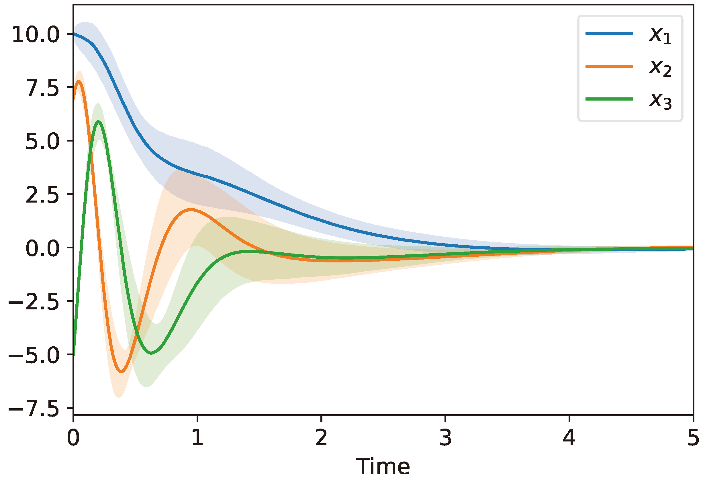
Example 1.

To illustrate the utility of Theorem 9, we showcase an example involving global stabilization of a stochastic version of the Lorentz equations [43]. These equations model fluid convection and are known to exhibit chaotic behavior. To construct inverse optimal controllers for the controlled Lorentz stochastic dynamical system consider the system

$$\begin{array}{ccc}\hfill \mathrm{d}{x}_1& =& [-\alpha x_1(t)+\alpha x_2(t)]\mathrm{d}t+{\sigma }_1{x}_1(t)\mathrm{d}w(t),x_1(0)=x_{10},t\ge 0,\hfill \end{array}$$

(99)

$$\begin{array}{ccc}\hfill \mathrm{d}{x}_2& =& [r{x}_1(t)-x_2(t)-x_1(t)x_3(t)+u(t)]\mathrm{d}t+{\sigma }_2{x}_2(t)\mathrm{d}w(t),x_2(0)=x_{20},\hfill \end{array}$$

(100)

$$\begin{array}{ccc}\hfill \mathrm{d}{x}_3& =& [x_1(t)x_2(t)-b{x}_3(t)]\mathrm{d}t+{\sigma }_3{x}_3(t)\mathrm{d}w(t),x_3(0)=x_{30},\hfill \end{array}$$

(101)

where $\alpha ,r,b,{\sigma }_1,{\sigma }_2$, and ${\sigma }_3>0$. Note that (99)–(101) can be written in the form of (81) with

$$f(x)=\left[\begin{array}{c}-\alpha x_1+\alpha x_2\\ r{x}_1-x_2-x_1{x}_3\\ x_1{x}_2-b{x}_3\end{array}\right],G(x)=\left[\begin{array}{c}0\\ 1\\ 0\end{array}\right],D(x)=\left[\begin{array}{c}{\sigma }_1{x}_1\\ {\sigma }_2{x}_2\\ {\sigma }_3{x}_3\end{array}\right].$$

In order to design an inverse optimal control law for the controlled Lorentz stochastic dynamical system (99)–(101) consider the quadratic Lyapunov function candidate given by

$$V(x)=p_1{x}_1^2+p_2{x}_2^2+p_3{x}_3^2,$$

(102)

where $x\stackrel{▵}{=}{[x_1,x_2,x_3]}^{\mathrm{T}}$ and $p_1,p_2,p_3>0$. Now, letting $p_2=p_3$, ${\sigma }_1<\sqrt{\alpha }$, $|{\sigma }_2|<1$, $|{\sigma }_3|<1$, and $L(x,u)=L_1(x)+L_2(x)u+R_2{u}^2$, where $R_2>0$, it follows that

$$L_2(x)=\frac{R_2}{p_2}(2p_1\alpha +2p_{2}r)x_1-2p_2{x}_2,$$

(103)

satisfies (88); that is,

$$\begin{array}{ccc}\hfill \mathcal{L}V(x)& =& V^{\prime }(x)[f(x)-\frac{1}{2}G(x)R_2^{-1}{L}_2^{\mathrm{T}}(x)-\frac{1}{2}G(x)R_2^{-1}{G}^{\mathrm{T}}(x)V^{\prime \mathrm{T}}(x)]\hfill \\ & & +\frac{1}{2}\mathrm{tr}{D}^{\mathrm{T}}(x)V^{″}(x)D(x)\hfill \\ & =& -2[(\alpha -{\sigma }_1^2)p_1{x}_1^2+(1-{\sigma }_2^2)p_2{x}_2^2+(1-{\sigma }_3^2)p_{2}b{x}_3^2]\hfill \\ & <& 0,x\in {\mathbb{R}}^3,x\ne 0.\hfill \end{array}$$

Hence, the feedback control law $\varphi (x)=-(\frac{p_1}{p_2}\alpha +r)x_1$ given by (90) globally stabilizes the controlled Lorentz dynamical system (99)–(101). Furthermore, the performance functional (83), with

$$L_1(x)=[2\sigma p_1+R_2{(\frac{p_1}{p_2}\alpha +r)}^2]x_1^2-2(p_1\sigma +p_{2}r)x_1{x}_2+2p_2{x}_2^2+2p_{2}b{x}_3^2,$$

(104)

is minimized in the sense of (92).

Figure 1 shows the mean along with the standard deviation of 1000 system sample paths with parameters $\alpha =r=b=1$, ${\sigma }_1={\sigma }_2={\sigma }_3=0.25$, and $p_1=p_2=p_3=1$. ▵

The next theorem is similar to Theorem 9 and is included here as it provides the basis for our stability margin results given in the next sections.

Theorem 10.

Consider the nonlinear controlled affine stochastic dynamical system (81) with performance measure (83). Assume that there exists a two-times continuously differentiable, radially unbounded function $V\in {\mathrm{C}}_{\mathrm{p}}^1({\mathbb{R}}^n)$ such that

$$\begin{array}{ccc}\hfill V(0)& =& 0,\hfill \end{array}$$

(105)

$$\begin{array}{ccc}\hfill V(x)& >& 0,x\in {\mathbb{R}}^n,x\ne 0,\hfill \end{array}$$

(106)

$$\begin{array}{c}{L}_2(0)=0,\\ V^{\prime }(x)[f(x)-\frac{1}{2}G(x)R_2^{-1}(x)L_2^{\mathrm{T}}(x)-\frac{1}{2}G(x)R_2^{-1}(x)G^{\mathrm{T}}(x)V^{\prime \mathrm{T}}(x)]\end{array}$$

(107)

$$\begin{array}{c}+\frac{1}{2}\mathrm{tr}{D}^{\mathrm{T}}(x)V^{″}(x)D(x)<0,x\in {\mathbb{R}}^n,x\ne 0,\\ 0=L_1(x)+V^{\prime }(x)f(x)+\frac{1}{2}\mathrm{tr}{D}^{\mathrm{T}}(x)V^{″}(x)D(x)-\frac{1}{4}[V^{\prime }(x)G(x)+L_2(x)]\end{array}$$

(108)

$$\begin{array}{c}·R_2^{-1}(x){[V^{\prime }(x)G(x)+L_2(x)]}^{\mathrm{T}},x\in {\mathbb{R}}^n.\end{array}$$

(109)

Then the zero solution $x(·)\equiv 0$ of the closed-loop system

$$\mathrm{d}x(t)=\left[f(x(t))+G(x(t))\varphi (x(t))\right]\mathrm{d}t+D(x(t))\mathrm{d}w(t),x(0)=x_0,t\ge 0,$$

(110)

is globally asymptotically stable in probability with the feedback control law

$$\varphi (x)=-\frac{1}{2}{R}_2^{-1}(x){[V^{\prime }(x)G(x)+L_2(x)]}^{\mathrm{T}},$$

(111)

and the performance functional (83) is minimized in the sense that

$$J(x_0,\varphi (x(·)))=\underset{u(·)\in \mathcal{S}(x_0)}{min}J(x_0,u(·)),x_0\in {\mathbb{R}}^n.$$

(112)

Finally,

$$J(x_0,\varphi (x(·)))=V(x_0),x_0\in {\mathbb{R}}^n.$$

(113)

Proof. 

The proof is identical to the proof of Theorem 9 and, hence, is omitted. □

8. Relative Stability Margins for Optimal Nonlinear Stochastic Regulators

In this section, we establish relative stability margins for both optimal and inverse optimal nonlinear stochastic feedback regulators. Specifically, we derive sufficient conditions ensuring gain, sector, and disk margin guarantees for nonlinear stochastic dynamical systems under the control of nonlinear optimal and inverse optimal Hamilton–Jacobi–Bellman controllers. These controllers aim to minimize a nonlinear-nonquadratic performance criterion that includes cross-weighting terms. In the scenario where the cross-weighting term in the performance criterion is omitted, our findings align with the gain, sector, and disk margins derived for the deterministic optimal control problem outlined in [25].

Alternatively, by retaining the cross-terms in the performance criterion and specializing the optimal nonlinear-nonquadratic problem to a stochastic linear-quadratic problem featuring a multiplicative noise disturbance, our results recover the corresponding gain and phase margins for the deterministic linear-quadratic optimal control problem as presented in [44]. Despite the observed degradation of gain, sector, and disk margins due to the inclusion of cross-weighting terms, the added flexibility afforded by these terms enables the assurance of optimal and inverse optimal nonlinear controllers that can exhibit superior transient performance as compared to meaningful inverse optimal controllers.

To develop relative stability margins for nonlinear stochastic regulators consider the nonlinear stochastic dynamical system $\mathcal{G}$ given by

$$\begin{array}{cc}\hfill \mathrm{d}x(t)& =\left[f(x(t))+G(x(t))u(t)\right]\mathrm{d}t+D(x(t))\mathrm{d}w(t),x(0)=x_0,t\ge 0,\hfill \end{array}$$

(114)

$$\begin{array}{cc}\hfill y(t)& =-\varphi (x(t)),\hfill \end{array}$$

(115)

where $f:{\mathbb{R}}^n\to {\mathbb{R}}^n$ satisfies $f(0)=0$, $G:{\mathbb{R}}^n\to {\mathbb{R}}^{n\times m}$, $D:{\mathbb{R}}^n\to {\mathbb{R}}^{n\times d}$ satisfies $D(0)=0$, and $\varphi :{\mathbb{R}}^n\to {\mathbb{R}}^m$ is an admissible feedback controller such that $\mathcal{G}$ is globally asymptotically stable in probability with $u=-y$, with a nonlinear-nonquadratic performance criterion

$$J(x_0,u(·))={\mathbb{E}}^{x_0}\left[{\int }_0^{\infty }[L_1(x(t))+L_2(x(t))u(t)+u^{\mathrm{T}}(t)R_2(x(t))u(t)]\mathrm{d}t\right],$$

(116)

where $L_1:{\mathbb{R}}^n\to \mathbb{R}$, $L_2:{\mathbb{R}}^n\to {\mathbb{R}}^{1\times m}$, and $R_2:{\mathbb{R}}^n\to {\mathbb{R}}^{m\times m}$ are given such that $R_2(x)>0$, $x\in {\mathbb{R}}^n$, and $L_2(0)=0$.

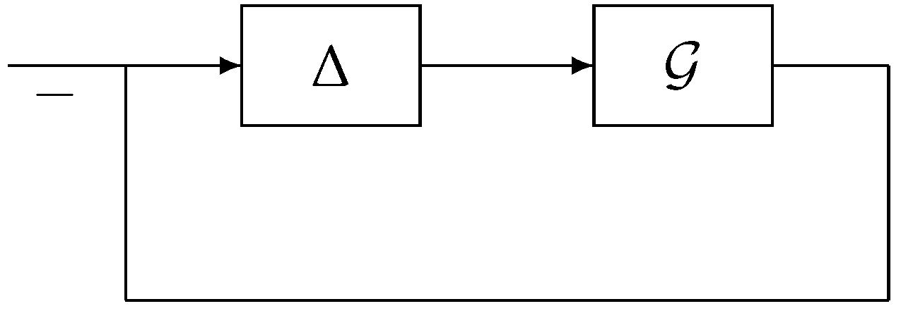
Next, we define the relative stability margins for $\mathcal{G}$ given by (114) and (115). Specifically, let $u_{\mathrm{c}}\stackrel{▵}{=}-y$, $y_{\mathrm{c}}\stackrel{▵}{=}u$, and consider the negative feedback interconnection $u=\Delta (-y)$ of $\mathcal{G}$ and $\Delta$ given in Figure 2, where $\Delta$ is either a linear operator $\Delta (u_{\mathrm{c}})=\Delta u_{\mathrm{c}}$, a nonlinear static operator $\Delta (u_{\mathrm{c}})=\sigma (u_{\mathrm{c}})$, or a nonlinear dynamic operator $\Delta$ with input $u_{\mathrm{c}}$ and output $y_{\mathrm{c}}$. Furthermore, we assume that in the nominal case $\Delta =I$ the nominal closed-loop system is globally asymptotically stable in probability.

Definition 3

([16]). Let $\alpha ,\beta \in \mathbb{R}$ be such that $0<\alpha \le 1\le \beta <\infty$. Then the nonlinear stochastic dynamical system $\mathcal{G}$ given by (114) and (115) is said to have a gain margin$(\alpha ,\beta )$ if the negative feedback interconnection of $\mathcal{G}$ and $\Delta (u_{\mathrm{c}})=\Delta u_{\mathrm{c}}$ is globally asymptotically stable in probability for all $\Delta =\mathrm{diag}[k_1,\dots ,k_m]$, where $k_i\in (\alpha ,\beta )$, $i=1,\dots ,m$.

Definition 4

([16]). Let $\alpha ,\beta \in \mathbb{R}$ be such that $0<\alpha \le 1\le \beta <\infty$. Then the nonlinear stochastic dynamical system $\mathcal{G}$ given by (114) and (115) is said to have a sector margin$(\alpha ,\beta )$ if the negative feedback interconnection of $\mathcal{G}$ and $\Delta (u_{\mathrm{c}})=\sigma (u_{\mathrm{c}})$ is globally asymptotically stable in probability for all nonlinearities $\sigma :{\mathbb{R}}^m\to {\mathbb{R}}^m$ such that $\sigma (0)=0$, $\sigma (u_{\mathrm{c}})={[{\sigma }_1(u_{\mathrm{c}1}),\dots ,{\sigma }_m(u_{\mathrm{c}m})]}^{\mathrm{T}}$, and $\alpha u_{\mathrm{c}i}^2<{\sigma }_i(u_{\mathrm{c}i})u_{\mathrm{c}i}<\beta u_{\mathrm{c}i}^2$, for all $u_{\mathrm{c}i}\ne 0$, $i=1,\dots ,m$.

Definition 5.

A nonlinear stochastic dynamical systems $\mathcal{G}$ is asymptotically zero-state observable if ${lim}_{t\to \infty }u(t)=0$ and ${lim}_{t\to \infty }y(t)=0$ imply ${lim}_{t\to \infty }x(t)=0$.

For the next two definitions, we assume that the system $\mathcal{G}$ and the nonlinear operator $\Delta$ are asymptotically zero-state observable.

Definition 6

([16]). Let $\alpha ,\beta \in \mathbb{R}$ be such that $0<\alpha \le 1\le \beta <\infty$. Then the nonlinear stochastic dynamical system $\mathcal{G}$ given by (114) and (115) is said to have a disk margin$(\alpha ,\beta )$ if the negative feedback interconnection of $\mathcal{G}$ and Δ is globally asymptotically stable in probability for all dynamic operators Δ such that Δ is stochastically dissipative with respect to the supply rate $r_{\mathrm{c}}(u_{\mathrm{c}},y_{\mathrm{c}})=u_{\mathrm{c}}^{\mathrm{T}}{y}_{\mathrm{c}}-\frac{1}{\widehat{\alpha }+\widehat{\beta }}{y}_{\mathrm{c}}^{\mathrm{T}}{y}_{\mathrm{c}}-\frac{\widehat{\alpha }\widehat{\beta }}{\widehat{\alpha }+\widehat{\beta }}{u}_{\mathrm{c}}^{\mathrm{T}}{u}_{\mathrm{c}}$ and with a two-times continuously differentiable, positive definite storage function, where $\widehat{\alpha }=\alpha +\delta$, $\widehat{\beta }=\beta -\delta$, and $\delta \in \mathbb{R}$ such that $0<2\delta <\beta -\alpha$.

Definition 7

([16]). Let $\alpha ,\beta \in \mathbb{R}$ be such that $0<\alpha \le 1\le \beta <\infty$. Then the nonlinear stochastic dynamical system $\mathcal{G}$ given by (114) and (115) is said to have a structured disk margin$(\alpha ,\beta )$ if the negative feedback interconnection of $\mathcal{G}$ and Δ is globally asymptotically stable in probability for all dynamic operators Δ such that $\Delta (u_{\mathrm{c}})=\mathrm{diag}[{\delta }_1(u_{\mathrm{c}1}),\dots ,{\delta }_m(u_{\mathrm{c}m})]$, and ${\delta }_i$, $i=1,\dots ,m$, is stochastically dissipative with respect to the supply rate $r_{\mathrm{c}i}(u_{\mathrm{c}i},y_{\mathrm{c}i})=u_{\mathrm{c}i}{y}_{\mathrm{c}i}-\frac{1}{\widehat{\alpha }+\widehat{\beta }}{y}_{\mathrm{c}i}^2-\frac{\widehat{\alpha }\widehat{\beta }}{\widehat{\alpha }+\widehat{\beta }}{u}_{\mathrm{c}i}^2$ and with a two-times continuously differentiable, positive definite storage function, where $\widehat{A}\alpha =\alpha +\delta$, $\widehat{\beta }=\beta -\delta$, and $\delta \in \mathbb{R}$ such that $0<2\delta <\beta -\alpha$.

Note that if $\mathcal{G}$ has a disk margin $(\alpha ,\beta )$, then $\mathcal{G}$ has gain and sector margins $(\alpha ,\beta )$.

The following lemma is needed for developing the main results of this section.

Lemma 1.

Consider the nonlinear stochastic dynamical system $\mathcal{G}$ given by (114) and (115), where ϕ is a stochastically stabilizing feedback control law given by (111) and where V satisfies

$$\begin{array}{cc}\hfill 0& =V^{\prime }(x)f(x)+L_1(x)-\frac{1}{4}[V^{\prime }(x)G(x)+L_2(x)]R_2^{-1}(x){[V^{\prime }(x)G(x)+L_2(x)]}^{\mathrm{T}}\hfill \\ \hfill & +\frac{1}{2}\mathrm{tr}{D}^{\mathrm{T}}(x)V^{″}(x)D(x),x\in {\mathbb{R}}^n.\hfill \end{array}$$

(117)

Furthermore, suppose there exists $\theta \in \mathbb{R}$ such that $0<\theta <1$ and

$$(1-{\theta }^2)L_1(x)-\frac{1}{4}{L}_2(x)R_2^{-1}(x)L_2^{\mathrm{T}}(x)\ge 0,x\in {\mathbb{R}}^n.$$

(118)

Then,

$$\begin{array}{c}\hfill \mathcal{L}V(x)\le {[u+y]}^{\mathrm{T}}{R}_2(x)[u+y]-{\theta }^2{u}^{\mathrm{T}}{R}_2(x)u,\end{array}$$

(119)

for all $x\in {\mathbb{R}}^n$ and $u\in {\mathbb{R}}^m$.

Proof. 

Note that it follows from (117) and (118) that, for all $x\in {\mathbb{R}}^n$ and $u\in {\mathbb{R}}^m$,

$$\begin{array}{cc}\hfill {\theta }^2{u}^{\mathrm{T}}{R}_2(x)u& \le {\theta }^2{u}^{\mathrm{T}}{R}_2(x)u+\left[\frac{1}{2\sqrt{1-{\theta }^2}}{L}_2(x)R_2^{-1}(x)+\sqrt{1-{\theta }^2}{u}^{\mathrm{T}}\right]\hfill \\ \hfill & ·R_2(x){\left[\frac{1}{2\sqrt{1-{\theta }^2}}{L}_2(x)R_2^{-1}(x)+\sqrt{1-{\theta }^2}{u}^{\mathrm{T}}\right]}^{\mathrm{T}}\hfill \\ \hfill & =u^{\mathrm{T}}{R}_2(x)u+\frac{1}{4(1-{\theta }^2)}{L}_2(x)R_2^{-1}(x)L_2^{\mathrm{T}}(x)+L_2(x)u\hfill \\ \hfill & \le u^{\mathrm{T}}{R}_2(x)u+L_2(x)u+L_1(x)\hfill \\ \hfill & =u^{\mathrm{T}}{R}_2(x)u+L_2(x)u-V^{\prime }(x)f(x)\hfill \\ \hfill & +{\varphi }^{\mathrm{T}}(x)R_2(x)\varphi (x)-\frac{1}{2}\mathrm{tr}{D}^{\mathrm{T}}(x)V^{″}(x)D(x)\hfill \\ \hfill & ={[u+y]}^{\mathrm{T}}{R}_2(x)[u+y]-V^{\prime }(x)[f(x)+G(x)u]\hfill \\ \hfill & -\frac{1}{2}\mathrm{tr}{D}^{\mathrm{T}}(x)V^{″}(x)D(x),\hfill \end{array}$$

(120)

which implies that

$$\begin{array}{c}\hfill {\theta }^2{u}^{\mathrm{T}}{R}_2(x)u\le {[u+y]}^{\mathrm{T}}{R}_2(x)[u+y]-\mathcal{L}V(x).\end{array}$$

(121)

This completes the proof. □

Next, we present disk margins for the nonlinear-nonquadratic optimal regulator given by Theorem 10. We consider the case in which $R_2(x)$, $x\in {\mathbb{R}}^n$, is a constant diagonal matrix and the case in which it is not a constant diagonal matrix.

Theorem 11.

Consider the nonlinear stochastic dynamical system $\mathcal{G}$ given by (114) and (115), where ϕ is the stochastically stabilizing feedback control law given by (111) and where $V\in {\mathrm{C}}_{\mathrm{p}}^1({\mathbb{R}}^n)$ is a two-times continuously differentiable, radially unbounded function that satisfies (105)–(109). Assume that $\mathcal{G}$ is asymptotically zero state observable. If the matrix $R_2(x)=\mathrm{diag}[r_1,\dots ,r_m]$, where $r_i>0$, $i=1,\dots ,m$, and there exists $\theta \in \mathbb{R}$ such that $0<\theta <1$ and (118) is satisfied, then the nonlinear stochastic dynamical system $\mathcal{G}$ has a structured disk margin $(\frac{1}{1+\theta },\frac{1}{1-\theta })$. If, in addition, $R_2(x)\equiv I$ and there exists $\theta \in \mathbb{R}$ such that $0<\theta <1$ and (118) is satisfied, then the nonlinear stochastic dynamical system $\mathcal{G}$ has a disk margin $(\frac{1}{1+\theta },$$\frac{1}{1-\theta })$.

Proof. 

Note that it follows from Lemma 1 that

$$\begin{array}{c}\hfill \mathcal{L}V(x)\le {[u+y]}^{\mathrm{T}}{R}_2[u+y]-{\theta }^2{u}^{\mathrm{T}}{R}_{2}u.\end{array}$$

(122)

Hence, with the storage function $V_{\mathrm{s}}(x)=\frac{1}{2}V(x)$, it follows from that $\mathcal{G}$ is stochastically dissipative with respect to the supply rate $r(u,y)=u^{\mathrm{T}}{R}_{2}y+\frac{1-{\theta }^2}{2}{u}^{\mathrm{T}}{R}_{2}u+\frac{1}{2}{y}^{\mathrm{T}}{R}_{2}y$. Now, the result is a direct consequence of Definitions 6 and 7, and the stochastic version of Corollary 6.2 given in [16] with $\alpha =\frac{1}{1+\theta }$ and $\beta =\frac{1}{1-\theta }$. □

For the next result, define

$$\overline{\gamma }\stackrel{▵}{=}\underset{x\in {\mathbb{R}}^n}{sup}{\sigma }_{max}(R_2(x)),\underline{\gamma }\stackrel{▵}{=}\underset{x\in {\mathbb{R}}^n}{\inf }{\sigma }_{min}(R_2(x)),$$

(123)

where $R_2(x)$ is such that $\overline{\gamma }<\infty$ and $\underline{\gamma }>0$.

Theorem 12.

Consider the nonlinear stochastic dynamical system $\mathcal{G}$ given by (114) and (115), where ϕ is the stochastically stabilizing feedback control law given by (111) and where $V\in {\mathrm{C}}_{\mathrm{p}}^1({\mathbb{R}}^n)$ is a two-times continuously differentiable, radially unbounded function that satisfies (105)–(109). Assume that $\mathcal{G}$ is asymptotically zero-state observable. If there exists $\theta \in \mathbb{R}$ such that $0<\theta <1$ and (118) is satisfied, then the nonlinear stochastic system $\mathcal{G}$ has a disk margin $(\frac{1}{1+\eta \theta },\frac{1}{1-\eta \theta })$, where $\eta \stackrel{▵}{=}\sqrt{\underline{\gamma }/\overline{\gamma }}$.

Proof. 

It follows from Lemma 1 that

$$\begin{array}{cc}\hfill \mathcal{L}V(x)& \le {[u+y]}^{\mathrm{T}}{R}_2(x)[u+y]-{\theta }^2{u}^{\mathrm{T}}{R}_2(x)u\hfill \\ \hfill & \le \overline{\gamma }{[u+y]}^{\mathrm{T}}[u+y]-\underline{\gamma }{\theta }^2{u}^{\mathrm{T}}u.\hfill \end{array}$$

(124)

Thus, with the storage function $V_{\mathrm{s}}(x)=\frac{1}{2\underline{\gamma }}V(x)$, $\mathcal{G}$ is stochastically dissipative with respect to thesupply rate $r(u,y)=u^{\mathrm{T}}y+\frac{1-{\eta }^2{\theta }^2}{2}{u}^{\mathrm{T}}u+\frac{1}{2}{y}^{\mathrm{T}}y$. The result now is a direct consequence of Definition 6 and the stochastic version of Corollary 6.2 given in [16] with $\alpha =\frac{1}{1+\eta \theta }$ and $\beta =\frac{1}{1-\eta \theta }$. □

Next, we provide a result that guarantees sector and gain margins for the case in which $R_2(x)$, $x\in {\mathbb{R}}^n$, is diagonal.

Theorem 13.

Consider the nonlinear stochastic dynamical system $\mathcal{G}$ given by (114) and (115), where ϕ is the stochastically stabilizing feedback control law given by (111) and where $V\in {\mathrm{C}}_{\mathrm{p}}^1({\mathbb{R}}^n)$ is a two-times continuously differentiable, radially unbounded function that satisfies (105)–(109). Furthermore, let $R_2(x)=\mathrm{diag}[r_1(x),\dots ,r_m(x)]$, where $r_i:{\mathbb{R}}^n\to \mathbb{R}$, $r_i(x)>0$, $i=1,\dots ,m$. If there exists $\theta \in \mathbb{R}$ such that $0<\theta <1$ and

$$(1-{\theta }^2)L_1(x)-\frac{1}{4}{L}_2(x)R_2^{-1}(x)L_2^{\mathrm{T}}(x)>0,x\in {\mathbb{R}}^n,$$

(125)

then the nonlinear stochastic dynamical system $\mathcal{G}$ has a sector (and hence, gain) margin $(\frac{1}{1+\theta },$$\frac{1}{1-\theta })$.

Proof. 

Let $\Delta (-y)=\sigma (-y)$, where $\sigma :{\mathbb{R}}^m\to {\mathbb{R}}^m$ is a static nonlinearity such that $\sigma (0)=0$, $\sigma (v)={[{\sigma }_1(v_1),\dots ,{\sigma }_m(v_m)]}^{\mathrm{T}}$, and $\alpha v_i^2<{\sigma }_i(v_i)v_i<\beta v_i^2$, for all $v_i\ne 0$, $i=1,\dots ,m$, where $\alpha =\frac{1}{1+\theta }$ and $\beta =\frac{1}{1-\theta }$; or, equivalently, $({\sigma }_i(v_i)-\alpha v_i)({\sigma }_i(v_i)-\beta v_i)<0$, for all $v_i\ne 0$, $i=1,\dots ,m$. In this case, the closed-loop system (114) and (115) with $u=\sigma (-y)$ is given by

$$\mathrm{d}x(t)=[f(x(t))+G(x(t))\sigma (\varphi (x(t)))]\mathrm{d}t+D(x(t))\mathrm{d}w(t),x(0)=x_0,t\ge 0.$$

(126)

Next, consider the two-times continuously differentiable, radially unbounded function Lyapunov function candidate V satisfying (105)–(109) and let $\mathcal{L}V$ denote the Lyapunov infinitesimal generator of the closed-loop system (126). Now, it follows from (109) and (125) that

$$\begin{array}{cc}\hfill \mathcal{L}V(x)& =V^{\prime }(x)f(x)+V^{\prime }(x)G(x)\sigma (\varphi (x))+\frac{1}{2}\mathrm{tr}{D}^{\mathrm{T}}(x)V^{\prime \prime }(x)D(x)\hfill \\ \hfill & <V^{\prime }(x)f(x)+V^{\prime }(x)G(x)\sigma (\varphi (x))+\frac{1}{2}\mathrm{tr}{D}^{\mathrm{T}}(x)V^{\prime \prime }(x)D(x)+L_1(x)\hfill \\ \hfill & -\frac{1}{4(1-{\theta }^2)}{L}_2(x)R_2^{-1}(x)L_2^{\mathrm{T}}(x)\hfill \\ \hfill & +(1-{\theta }^2){\left[\sigma (\varphi (x))-\frac{1}{2(1-{\theta }^2)}{R}_2^{-1}(x)L_2^{\mathrm{T}}(x)\right]}^{\mathrm{T}}{R}_2(x)\hfill \\ \hfill & ·\left[\sigma (\varphi (x))-\frac{1}{2(1-{\theta }^2)}{R}_2^{-1}(x)L_2^{\mathrm{T}}(x)\right]\hfill \\ \hfill & =V^{\prime }(x)f(x)+L_1(x)+V^{\prime }(x)G(x)\sigma (\varphi (x))+\frac{1}{2}\mathrm{tr}{D}^{\mathrm{T}}(x)V^{\prime \prime }(x)D(x)\hfill \\ \hfill & +(1-{\theta }^2){\sigma }^{\mathrm{T}}(\varphi (x))R_2(x)\sigma (\varphi (x))-L_2(x)\sigma (\varphi (x))\hfill \\ \hfill & ={\varphi }^{\mathrm{T}}(x)R_2(x)\varphi (x)-2{\varphi }^{\mathrm{T}}(x)R_2(x)\sigma (\varphi (x))\hfill \\ \hfill & +(1-{\theta }^2){\sigma }^{\mathrm{T}}(\varphi (x))R_2(x)\sigma (\varphi (x))\hfill \\ \hfill & =\sum _{i=1}^m{r}_i(x)(\frac{1}{\beta }{\sigma }_i(-y_i)+y_i)(\frac{1}{\alpha }{\sigma }_i(-y_i)+y_i)\hfill \\ \hfill & =\frac{1}{\alpha \beta }\sum _{i=1}^m{r}_i(x)\left({\sigma }_i(-y_i)+\alpha y_i\right)\left({\sigma }_i(-y_i)+\beta y_i\right)\hfill \\ \hfill & <0,x\in {\mathbb{R}}^n,\hfill \end{array}$$

(127)

which, by Theorem 2, implies that the closed-loop system (126) is globally asymptotically stable in probability for all $\sigma$ such that $\alpha v_i^2<{\sigma }_i(v_i)v_i<\beta v_i^2$, $v_i\ne 0$, $i=1,\dots ,m$. Hence, $\mathcal{G}$ given by (114) and (115) has sector (and hence, gain) margins $(\alpha ,\beta )$. □

It is important to note that Theorem 13 also holds in the case where (125) is replaced with (118) and with the additional assumption that (118) is radially unbounded. To see this, note that (127) can be written as

$$\begin{array}{c}\hfill \begin{array}{cc}\mathcal{L}V(x)=\hfill & -[L_1(x)-\frac{1}{4(1-{\theta }^2)}{L}_2(x)R_2^{-1}(x)L_2^{\mathrm{T}}(x)]\hfill \\ \hfill & -(1-{\theta }^2){\left[\sigma (\varphi (x))+\frac{1}{2(1-{\theta }^2)}{R}_2^{-1}(x)L_2^{\mathrm{T}}(x)\right]}^{\mathrm{T}}{R}_2(x)\hfill \\ \hfill & ·\left[\sigma (\varphi (x))+\frac{1}{2(1-{\theta }^2)}{R}_2^{-1}(x)L_2^{\mathrm{T}}(x)\right]\hfill \\ \hfill & +\frac{1}{\alpha \beta }\sum _{i=1}^m{r}_i(x)\left({\sigma }_i(-y_i)+\alpha y_i\right)\left({\sigma }_i(-y_i)+\beta y_i\right)\hfill \\ \hfill & \le -W(x),x\in {\mathbb{R}}^n,\hfill \end{array}\end{array}$$

(128)

where

$$W(x)\triangleq L_1(x)-\frac{1}{4(1-{\theta }^2)}{L}_2(x)R_2^{-1}(x)L_2^{\mathrm{T}}(x).$$

In this case, the result follows from Theorem 3.1 of [45]. Furthermore, note that in the case where $R_2(x)$, $x\in {\mathbb{R}}^n$, is diagonal, Theorem 13 guarantees larger gain and sector margins to the gain and sector margin guarantees provided by Theorem 12. However, Theorem 13 does not provide disk margin guarantees.

9. Nonlinear Stochastic Feedback Regulators with Relative Stability Margins Guarantees

In this section, we give sufficient conditions that guarantee that a given nonlinear feedback controller has prespecified disk, sector, and gain margins.

Proposition 1.

Let $\theta \in (0,1)$ and let $R_2\in {\mathbb{R}}^{m\times m}$ be a positive-definite matrix. Consider the nonlinear stochastic dynamical system $\mathcal{G}$ given by (114) and (115), where ϕ is a stochastically stabilizing feedback control law. Then there exist functions $V:{\mathbb{R}}^n\to \mathbb{R}$, $L_1:{\mathbb{R}}^n\to \mathbb{R}$, and $L_2:{\mathbb{R}}^n\to {\mathbb{R}}^{1\times m}$ such that $\varphi (x)=-\frac{1}{2}{R}_2^{-1}{[V^{\prime }(x)G(x)+L_2(x)]}^{\mathrm{T}}$, $V\in {\mathrm{C}}_{\mathrm{p}}^1({\mathbb{R}}^n)$ is a two-times continuously differentiable, radially unbounded function such that $V(0)=0$, $V(x)>0$, $x\in {\mathbb{R}}^n$, $x\ne 0$, and, for all $x\in {\mathbb{R}}^n$,

$$\begin{array}{cc}\hfill 0=& V^{\prime }(x)f(x)+L_1(x)-\frac{1}{4}[V^{\prime }(x)G(x)+L_2(x)]R_2^{-1}{[V^{\prime }(x)G(x)+L_2(x)]}^{\mathrm{T}}\hfill \\ \hfill & +\frac{1}{2}\mathrm{tr}{D}^{\mathrm{T}}(x)V^{″}(x)D(x),\hfill \end{array}$$

(129)

$$\begin{array}{cc}\hfill 0& \le (1-{\theta }^2)L_1(x)-\frac{1}{4}{L}_2(x)R_2^{-1}{L}_2^{\mathrm{T}}(x),\hfill \end{array}$$

(130)

if and only if there exists a two-times continuously differentiable, radially unbounded function $V\in {\mathrm{C}}_{\mathrm{p}}^1({\mathbb{R}}^n)$ such that $V(0)=0$, $V(x)>0$, $x\in {\mathbb{R}}^n$, $x\ne 0$, and

$$\begin{array}{c}\hfill \mathcal{L}V(x)\le {[u+y]}^{\mathrm{T}}{R}_2(x)[u+y]-{\theta }^2{u}^{\mathrm{T}}{R}_2(x)u,x\in {\mathbb{R}}^n,u\in {\mathbb{R}}^m.\end{array}$$

(131)

Proof. 

If there exist functions $V:{\mathbb{R}}^n\to \mathbb{R}$, $L_1:{\mathbb{R}}^n\to \mathbb{R}$, and $L_2:{\mathbb{R}}^n\to {\mathbb{R}}^{1\times m}$ such that $\varphi (x)=-\frac{1}{2}{R}_2^{-1}{[V^{\prime }(x)G(x)+L_2(x)]}^{\mathrm{T}}$ and (129) and (130) are satisfied, then it follows from Lemma 1 that (131) is satisfied.

Conversely, if (131) is satisfied, then with $Q=R_2$, $S=R_2$, and $R=(1-{\theta }^2)R_2$, it follows from the stochastic version of Theorem 5.6 of [16] that, for all $x\in {\mathbb{R}}^n$,

$$\begin{array}{cc}\hfill 0& \ge V^{\prime }(x)f(x)+\frac{1}{2}\mathrm{tr}{D}^{\mathrm{T}}(x)V^{″}(x)D(x)-{\varphi }^{\mathrm{T}}(x)R_2\varphi (x)\hfill \\ \hfill & +\frac{1}{4(1-{\theta }^2)}[2{\varphi }^{\mathrm{T}}(x)R_2+V^{\prime }(x)G(x)]R_2^{-1}{[2{\varphi }^{\mathrm{T}}(x)R_2+V^{\prime }(x)G(x)]}^{\mathrm{T}}.\hfill \end{array}$$

The result now follows with

$$L_1(x)=-V^{\prime }(x)f(x)+{\varphi }^{\mathrm{T}}(x)R_2\varphi (x)-\frac{1}{2}\mathrm{tr}{D}^{\mathrm{T}}(x)V^{″}(x)D(x)$$

and $L_2(x)$$=-[2{\varphi }^{\mathrm{T}}(x)R_2+V^{\prime }(x)G(x)]$. □

Note that if (129) and (130) are satisfied, then it follows from Theorem 9 that the feedback control law $\varphi (x)=-\frac{1}{2}{R}_2^{-1}{[V^{\prime }(x)G(x)+L_2(x)]}^{\mathrm{T}}$ minimizes the cost functional (83). Hence, Proposition 1 provides necessary and sufficient conditions for optimality of a given stochastically stabilizing feedback control law with prespecified disk margin guarantees.

The following result presents specific disk margin guarantees for inverse optimal controllers.

Theorem 14.

Let $\theta \in (0,1)$ be given. Consider the nonlinear stochastic dynamical system $\mathcal{G}$ given by (114) and (115), where ϕ is a stochastically stabilizing feedback control law. Assume that $\mathcal{G}$ is asymptotically zero-state observable, there exist functions $V:{\mathbb{R}}^n\to \mathbb{R}$ and $R_2:{\mathbb{R}}^n\to {\mathbb{R}}^{m\times m}$ such that $V\in {\mathrm{C}}_{\mathrm{p}}^1({\mathbb{R}}^n)$ is a two-times continuously differentiable, radially unbounded function, $R_2(x)>0$, $x\in {\mathbb{R}}^n$, and

$$\begin{array}{c}V(0)=0,\end{array}$$

(132)

$$\begin{array}{c}V(x)>0,x\in {\mathbb{R}}^n,x\ne 0,\end{array}$$

(133)

$$\begin{array}{c}{V}^{\prime }(x)[f(x)+G(x)\varphi (x)]+\frac{1}{2}\mathrm{tr}{D}^{\mathrm{T}}(x)V^{″}(x)D(x)<0,x\in {\mathbb{R}}^n,x\ne 0,\\ V^{\prime }(x)f(x)+\frac{1}{2}\mathrm{tr}{D}^{\mathrm{T}}(x)V^{″}(x)D(x)-{\varphi }^{\mathrm{T}}(x)R_2^{-1}(x)\varphi (x)\\ +\frac{1}{1-{\theta }^2}\left({\varphi }^{\mathrm{T}}(x)+\frac{1}{2}{V}^{\prime }(x)G(x)R_2^{-1}(x)\right)R_2(x)\end{array}$$

(134)

$$\begin{array}{c}·{\left({\varphi }^{\mathrm{T}}(x)+\frac{1}{2}{V}^{\prime }(x)G(x)R_2^{-1}(x)\right)}^{\mathrm{T}}\le 0,x\in {\mathbb{R}}^n.\end{array}$$

(135)

Then the nonlinear stochastic dynamical system $\mathcal{G}$ has a disk margin $(\frac{1}{1+\eta \theta },\frac{1}{1-\eta \theta })$, where $\eta =\sqrt{\underline{\gamma }/\overline{\gamma }}$ and $\underline{\gamma }$ and $\overline{\gamma }$ are given by (123). Furthermore, with the feedback control law ϕ the performance functional

$$\begin{array}{cc}\hfill J(x_0,u(·))& ={\mathbb{E}}^{x_0}[{\int }_0^{\infty }[-V^{\prime }(x(t))(f(x(t))+G(x(t))u(t))\hfill \\ \hfill & +{(\varphi (x(t))-u(t))}^{\mathrm{T}}{R}_2(x(t))(\varphi (x(t))-u(t))\left]\mathrm{d}t\right]\hfill \end{array}$$

(136)

is minimized in the sense that

$$J(x_0,\varphi (x(·)))=\underset{u(·)\in \mathcal{S}(x_0)}{min}J(x_0,u(·)),x_0\in {\mathbb{R}}^n.$$

(137)

Proof. 

The result is a direct consequence of Theorems 9 and 12 with $L_1(x)=-V^{\prime }(x)f(x)+{\varphi }^{\mathrm{T}}(x)R_2(x)\varphi (x)-\frac{1}{2}\mathrm{tr}{D}^{\mathrm{T}}(x)V^{″}(x)D(x)$ and $L_2(x)=-(2{\varphi }^{\mathrm{T}}(x)R_2(x)+V^{\prime }(x)G(x))$. Specifically, in this case, all the conditions of Theorem 9 are trivially satisfied. Furthermore, note that (135) is equivalent to (118). The result now follows from Theorems 9 and 12. □

The next result provides sufficient conditions that guarantee that a given nonlinear feedback controller has prespecified gain and sector margins.

Theorem 15.

Let $\theta \in (0,1)$ be given. Consider the asymptotically zero-state observable nonlinear stochastic dynamical system $\mathcal{G}$ given by (114) and (115), where ϕ is a stochastically stabilizing feedback control law. Assume there exist functions $R_2(x)=\mathrm{diag}[r_1(x),\dots ,r_m(x)]$, where $r_i:{\mathbb{R}}^n\to \mathbb{R}$, $r_i(x)>0$, $i=1,\dots ,m$, and $V\in {\mathrm{C}}_{\mathrm{p}}^1({\mathbb{R}}^n)$ is a two-times continuously differentiable, radially unbounded function, and satisfies (132)–(135). Then the nonlinear stochastic dynamical system $\mathcal{G}$ has a disk margin $(\frac{1}{1+\theta },\frac{1}{1-\theta })$. Furthermore, with the feedback control law ϕ the performance functional (136) is minimized in the sense that

$$J(x_0,\varphi (x(·)))=\underset{u(·)\in \mathcal{S}(x_0)}{min}J(x_0,u(·)),x_0\in {\mathbb{R}}^n.$$

(138)

Proof. 

The result is a direct consequence of Theorems 9 and 13 with the proof being identical to the proof of Theorem 14. □

10. Optimal Linear-Quadratic Stochastic Control

In this section, we specialize Theorems 11 and 12 to the case of linear stochastic systems with multiplicative disturbance noise. Specifically, consider the stabilizable stochastic linear system given by

$$\begin{array}{ccc}\hfill \mathrm{d}x(t)& =& [Ax(t)+Bu(t)]\mathrm{d}t+x{\sigma }^{\mathrm{T}}\mathrm{d}w(t),x(0)=x_0,t\ge 0,\hfill \end{array}$$

(139)

$$\begin{array}{ccc}\hfill y(t)& =& -Kx(t),\hfill \end{array}$$

(140)

where $A\in {\mathbb{R}}^{n\times n}$, $B\in {\mathbb{R}}^{n\times m}$, $K\in {\mathbb{R}}^{m\times n}$, and $\sigma \in {\mathbb{R}}^d$, and assume that $(A,K)$ is detectable and the system (139) and (140) is asymptotically stable in probability with the feedback $u=-y$ or, equivalently, $\tilde{A}+BK$ is Hurwitz, where $\tilde{A}=A+\frac{1}{2}{\Vert \sigma \Vert }^2{I}_n$. Furthermore, assume that K is an optimal regulator that minimizes the quadratic performance functional given by

$$J(x_0,u(·))={\mathbb{E}}^{x_0}\left[{\int }_0^{\infty }[x^{\mathrm{T}}(t)R_{1}x(t)+2x^{\mathrm{T}}(t)R_{12}u(t)+u^{\mathrm{T}}(t)R_{2}u(t)]\mathrm{d}t\right],$$

(141)

where $R_1\in {\mathbb{R}}^{n\times n}$, $R_{12}\in {\mathbb{R}}^{n\times m}$, and $R_2\in {\mathbb{R}}^{m\times m}$ are such that $R_2>0$, $R_1-R_{12}{R}_2^{-1}{R}_{12}^{\mathrm{T}}\ge 0$, and $(A,R_1)$ is observable. In this case, it follows from Theorem 9 with $f(x)=Ax$, $G(x)=B$, $L_1(x)=x^{\mathrm{T}}{R}_{1}x$, $L_2(x)=2x^{\mathrm{T}}{R}_{12}$, $R_2(x)=R_2$, $\varphi (x)=Kx$, and $V(x)=x^{\mathrm{T}}Px$ that the optimal control law K is given by $K=-R_2^{-1}(B^{\mathrm{T}}P+R_{12})$, where $P>0$ is the solution to the algebraic regulator Riccati equation given by

$$0={(\tilde{A}-B{R}_2^{-1}{R}_{12}^{\mathrm{T}})}^{\mathrm{T}}P+P(\tilde{A}-B{R}_2^{-1}{R}_{12}^{\mathrm{T}})+R_1-R_{12}{R}_2^{-1}{R}_{12}^{\mathrm{T}}-PB{R}_2^{-1}{B}^{\mathrm{T}}P.$$

(142)

The following results provide guarantees of disk, sector, and gain margins for the system (139) and (140). We assume that $\mathcal{G}$ is asymptotically zero-state observable.

Corollary 3.

Consider the stochastic dynamical system with multiplicative noise given by (139) and (140) and with performance functional (141), and let ${\sigma }_{max}^2(R_{12})<{\sigma }_{min}(R_1){\sigma }_{min}(R_2)$. Then, with $K=-R_2^{-1}(B^{\mathrm{T}}P$$+R_{12})$, where $P>0$ satisfies (142), the system (139) and (140) has disk margin (and, hence, sector and gain margins) $(\frac{1}{1+\eta \theta },\frac{1}{1-\eta \theta })$, where

$$\eta =\frac{{\sigma }_{min}(R_2)}{{\sigma }_{max}(R_2)},\theta ={\left(1-\frac{{\sigma }_{max}^2(R_{12})}{{\sigma }_{min}(R_1){\sigma }_{min}(R_2)}\right)}^{1/2}.$$

(143)

Proof. 

The result is a direct consequence of Theorem 12 with $f(x)=Ax$, $G(x)=B$, $\varphi (x)=Kx$, $V(x)=x^{\mathrm{T}}Px$, $L_1(x)=x^{\mathrm{T}}{R}_{1}x$, and $L_2(x)=2x^{\mathrm{T}}{R}_{12}$. Specifically, note that (142) is equivalent to (109). Now, with $\theta$ given by (143), it follows that $(1-{\theta }^2)R_1-R_{12}{R}_2^{-1}{R}_{12}^{\mathrm{T}}\ge 0$, and hence, (118) is satisfied so that all the conditions of Theorem 12 are satisfied. □

Corollary 4.

Consider the stochastic dynamical system with multiplicative noise given by (139) and (140) and with performance functional (141), and let ${\sigma }_{max}^2(R_{12})<{\sigma }_{min}(R_1){\sigma }_{min}(R_2)$, where $R_2$ is diagonal. Then, with $K=-R_2^{-1}(B^{\mathrm{T}}P+R_{12})$, where $P>0$ satisfies (142), the system (139) and (140) has structured disk margin (and hence, gain and sector) margin $(\frac{1}{1+\theta },\frac{1}{1-\theta })$, where

$$\theta ={\left(1-\frac{{\sigma }_{max}^2(R_{12})}{{\sigma }_{min}(R_1){\sigma }_{min}(R_2)}\right)}^{1/2}.$$

(144)

Proof. 

The result is a direct consequence of Theorem 11 with $f(x)=Ax$, $G(x)=B$, $\varphi (x)=Kx$, $V(x)=x^{\mathrm{T}}Px$, $L_1(x)=x^{\mathrm{T}}{R}_{1}x$, and $L_2(x)=2x^{\mathrm{T}}{R}_{12}$. Specifically, note that (142) is equivalent to (109). Now, with $\theta$ given by (144), it follows that $(1-{\theta }^2)R_1-R_{12}{R}_2^{-1}{R}_{12}^{\mathrm{T}}\ge 0$, and hence, (118) is satisfied so that all the conditions of Theorem 11 are satisfied. □

The gain margins specified in Corollary 4 precisely match those presented in [44] for deterministic linear-quadratic optimal regulators incorporating cross-weighting terms in the performance criterion. Additionally, as Corollary 4 ensures structured disk margins of $(\frac{1}{1+\theta },\frac{1}{1-\theta })$, it implies that the system possesses a phase margin $\varphi$ defined as follows:

$$cos(\varphi )=1-\frac{{\theta }^2}{2},$$

(145)

or equivalently,

$$sin\left(\frac{\varphi }{2}\right)=\frac{\theta }{2}.$$

(146)

In the scenario where $R_{12}=0$, deduced from (144), it follows that $\theta =1$. Consequently, Corollary 4 ensures a phase margin of $\pm {60}^{\circ }$ in each input–output channel. Additionally, stipulating $R_1\ge 0$ leads to the conclusion, based on Corollary 4, that the system described by (139) and (140) possesses a gain and sector margin of $(\frac{1}{2},\infty )$.

11. Stability Margins and Meaningful Inverse Optimality

In this section, we establish explicit links between stochastic stability margins, stochastic meaningful inverse optimality, and stochastic dissipativity, focusing on a specific quadratic supply rate. More precisely, we derive a stochastic counterpart to the classical return difference inequality for continuous-time systems with continuously differentiable flows [21,46] in the context of stochastic dynamical systems. Furthermore, we establish connections between stochastic dissipativity and optimality for stochastic nonlinear controllers. Notably, we demonstrate the equivalence between stochastic dissipativity and optimality in the realm of stochastic dynamical systems. Specifically, we illustrate that an optimal nonlinear feedback controller $\varphi$, satisfying a return difference condition based on the infinitesimal generator of a controlled Markov diffusion process, is equivalent to the stochastic dynamical system—with input u and output $y=-\varphi (x)$—being stochastically dissipative with respect to a supply rate expressed as ${[u+y]}^{\mathrm{T}}[u+y]-u^{\mathrm{T}}u$.

Here, we assume that $L(x,u)$ is nonnegative for all $(x,u)\in {\mathbb{R}}^n\times {\mathbb{R}}^m$, which, in the terminology of [25,47], corresponds to a meaningful cost functional. Furthermore, we assume $L_2(x)\equiv 0$ and $L_1(x)\ge 0$, $x\in {\mathbb{R}}^n$, and is radially unbounded. In this case, we establish connections between stochastic dissipativity and optimality for nonlinear stochastic controllers. The first result specializes Theorem 10 to the case in which $L_2(x)\equiv 0$.

Theorem 16.

Consider the nonlinear stochastic dynamical system (114) with performance functional (83) with $L_2(x)\equiv 0$ and $L_1(x)\ge 0$, $x\in {\mathbb{R}}^n$. Assume that there exists a two-times continuously differentiable, radially unbounded function $V\in {\mathrm{C}}_{\mathrm{p}}^1({\mathbb{R}}^n)$ such that

$$\begin{array}{c}V(0)=0,\end{array}$$

(147)

$$\begin{array}{c}V(x)>0,x\in {\mathbb{R}}^n,x\ne 0,\\ 0=L_1(x)+V^{\prime }(x)f(x)+\frac{1}{2}\mathrm{tr}{D}^{\mathrm{T}}(x)V^{″}(x)D(x)\end{array}$$

(148)

$$\begin{array}{c}-\frac{1}{4}{V}^{\prime }(x)G(x)R_2^{-1}(x)G^{\mathrm{T}}(x)V^{\prime \mathrm{T}}(x),x\in {\mathbb{R}}^n.\end{array}$$

(149)

Then the zero solution $x(·)\equiv 0$ of the closed-loop system

$$\mathrm{d}x(t)=[f(x(t))+G(x(t))\varphi (x(t))]\mathrm{d}t+D(x(t))\mathrm{d}w(t),x(0)=x_0,t\ge 0.$$

(150)

is globally asymptotically stable in probability with the feedback control law

$$\varphi (x)=-\frac{1}{2}{R}_2^{-1}(x)G^{\mathrm{T}}(x)V^{\prime \mathrm{T}}(x),$$

(151)

and the performance functional (83) is minimized in the sense that

$$J(x_0,\varphi (x(·)))=\underset{u(·)\in \mathcal{S}(x_0)}{min}J(x_0,u(·)),x_0\in {\mathbb{R}}^n.$$

(152)

Finally,

$$J(x_0,\varphi (x(·)))=V(x_0),x_0\in {\mathbb{R}}^n.$$

(153)

Proof. 

The proof is similar to the proof of Theorem 9, and hence, is omitted. □

Next, we show that for a given nonlinear stochastic dynamical system $\mathcal{G}$ given by (114) and (115), there exists an equivalence between optimality and stochastic dissipativity. For the following result we assume that for a given nonlinear stochastic system (114), if there exists a feedback control law $\varphi$ that minimizes the performance functional (83) with $R_2(x)\equiv I$, $L_2(x)\equiv 0$, and $L_1(x)\ge 0$, $x\in {\mathbb{R}}^n$, then there exists a two-times continuously differentiable, radially unbounded function $V\in {\mathrm{C}}_{\mathrm{p}}^1({\mathbb{R}}^n)$ such that (149) is satisfied.

Theorem 17.

Consider the nonlinear stochastic dynamical system $\mathcal{G}$ given by (114) and (115). The feedback control law $u=\varphi (x)$ is optimal with respect to a performance functional (82) with $R_2(x)\equiv I$, $L_2(x)\equiv 0$, and $L_1(x)\ge 0$, $x\in {\mathbb{R}}^n$, if and only if the nonlinear stochastic system $\mathcal{G}$ is stochastically dissipative with respect to the supply rate $r(u,y)=y^{\mathrm{T}}y+2u^{\mathrm{T}}y$ and has a two-times continuously differentiable positive-definite, radially unbounded storage function $V\in {\mathrm{C}}_{\mathrm{p}}^1({\mathbb{R}}^n)$.

Proof. 

If the control law $\varphi$ is optimal with respect to a performance functional (82) with $R_2(x)\equiv I$, $L_2(x)\equiv 0$, and $L_1(x)\ge 0$, $x\in {\mathbb{R}}^n$, then, by assumption, there exists a two-times continuously differentiable, radially unbounded function $V\in {\mathrm{C}}_{\mathrm{p}}^1({\mathbb{R}}^n)$ such that (149) is satisfied. Hence, it follows from Proposition 1 that

$$\begin{array}{c}\hfill \mathcal{L}V(x)\le {[u+y]}^{\mathrm{T}}{R}_2(x)[u+y]-{\theta }^2{u}^{\mathrm{T}}{R}_2(x)u,\end{array}$$

(154)

which implies that $\mathcal{G}$ is stochastically dissipative with respect to the supply rate $r(u,y)=y^{\mathrm{T}}y+2u^{\mathrm{T}}y$.

Conversely, if $\mathcal{G}$ is stochastically dissipative with respect to the supply rate $r(u,y)=y^{\mathrm{T}}y+2u^{\mathrm{T}}y$ and has a two-times continuously differentiable positive-definite storage function $V\in {\mathrm{C}}_{\mathrm{p}}^1({\mathbb{R}}^n)$, then, with $h(x)=-\varphi (x)$, $J(x)\equiv 0$, $Q=I$, $R=0$, and $S=2I$, it follows from the stochastic version of Theorem 5.6 of [16] that there exists a function $\ell :{\mathbb{R}}^n\to {\mathbb{R}}^p$ such that $\varphi (x)=-\frac{1}{2}{G}^{\mathrm{T}}(x)V^{\prime \mathrm{T}}(x)$ and, for all $x\in {\mathbb{R}}^n$,

$$0=V^{\prime }(x)f(x)+\frac{1}{2}\mathrm{tr}{D}^{\mathrm{T}}(x)V^{″}(x)D(x)-\frac{1}{4}{V}^{\prime }(x)G(x)G^{\mathrm{T}}(x)V^{\prime \mathrm{T}}(x)+{\ell }^{\mathrm{T}}(x)\ell (x).$$

Now, the result follows from Theorem 16 with $L_1(x)={\ell }^{\mathrm{T}}(x)\ell (x)$. □

The next result gives disk and structured disk margins for the nonlinear stochastic dynamical system $\mathcal{G}$ given by (114) and (115).

Corollary 5.

Consider the nonlinear stochastic dynamical system $\mathcal{G}$ given by (114) and (115), where ϕ is the stochastically stabilizing feedback control law given by (111) with $L_2(x)\equiv 0$ and where $V\in {\mathrm{C}}_{\mathrm{p}}^1({\mathbb{R}}^n)$ is a two-times continuously differentiable, radially unbounded function that satisfies (105)–(109). Assume that $\mathcal{G}$ is asymptotically zero state observable. Furthermore, assume $R_2(x)=\mathrm{diag}[r_1,\dots ,r_m]$, where $r_i>0$, $i=1,\dots ,m$, and $L_1(x)\ge 0$, $x\in {\mathbb{R}}^n$. Then the nonlinear stochastic dynamical system $\mathcal{G}$ has a structured disk margin $(\frac{1}{2},\infty )$. If, in addition, $R_2(x)\equiv I_m$, then the nonlinear stochastic system $\mathcal{G}$ has a disk margin $(\frac{1}{2},\infty )$

Proof. 

The result is a direct consequence of Theorem 11. Specifically, if $L_1(x)\ge 0$, $x\in {\mathbb{R}}^n$, and $L_2(x)\equiv 0$, then (118) is trivially satisfied for all $\theta \in (0,1)$. Now, the result follows immediately by letting $\theta \to 1$. □

Finally, we provide sector and gain margins for the nonlinear stochastic dynamical system $\mathcal{G}$ given by (114) and (115).

Corollary 6.

Consider the nonlinear stochastic dynamical system $\mathcal{G}$ given by (114) and (115), where ϕ is a stochastically stabilizing feedback control law given by (111) with $L_2(x)\equiv 0$ and where $V\in {\mathrm{C}}_{\mathrm{p}}^1({\mathbb{R}}^n)$ is a two-times continuously differentiable, radially unbounded function that satisfies (105)–(109). Furthermore, assume $R_2(x)=\mathrm{diag}[r_1(x),$$\dots ,r_m(x)]$, where $r_i:{\mathbb{R}}^n\to \mathbb{R}$, $r_i(x)>0$, $i=1,\dots ,m$, and $L_1(x)>0$, $x\in {\mathbb{R}}^n$. Then the nonlinear stochastic dynamical system $\mathcal{G}$ has a sector (and hence, gain) margin $(\frac{1}{2},\infty )$.

Proof. 

The result is a direct consequence of Theorem 13. Specifically, if $L_1(x)>0$, $x\in {\mathbb{R}}^n$, and $L_2(x)\equiv 0$, then (125) is trivially satisfied for all $\theta \in (0,1)$. Now, the result follows immediately by letting $\theta \to 1$. □

12. Conclusions

In this paper, we merged stochastic Lyapunov theory with stochastic Hamilton–Jacobi–Bellman theory to provide explicit connections between stability and optimality of nonlinear stochastic regulators. The proposed approach involves utilizing a steady-state stochastic Hamilton–Jacobi–Bellman framework to characterize optimal nonlinear feedback controllers wherein the notion of optimality is directly linked to a specified Lyapunov function, guaranteeing stability in probability for the closed-loop system. The derived results are then employed to establish inverse optimal feedback controllers for both affine nonlinear stochastic systems and linear stochastic systems.

Moreover, leveraging the concepts of stochastic stability and stochastic dissipativity theory, we developed sufficient conditions for gain, sector, and disk margin guarantees. These conditions apply to nonlinear stochastic dynamical systems controlled by both nonlinear optimal and inverse optimal regulators, minimizing a nonlinear-nonquadratic performance criterion. Furthermore, we established connections between stochastic dissipativity and optimality for nonlinear stochastic systems. The novelty of the proposed framework provides the foundation for extending linear-quadratic control for stochastic dynamical systems to nonlinear-nonquadratic problems.

References

1. Baumann, W.T.; Rugh, W.J. Feedback control of nonlinear systems by extended linearization. IEEE Trans. Autom. Control 1986, 31, 40–46. [Google Scholar] [CrossRef]
2. Wang, J.; Rugh, W.J. Feedback linearization families for nonlinear systems. IEEE Trans. Autom. Control 1987, 32, 935–941. [Google Scholar] [CrossRef]
3. Blueschke, D.; Blueschke-Nikolaeva, V.; Neck, R. Approximately optimal control of nonlinear dynamic stochastic problems with learning: The OPTCON algorithm. Algorithms 2021, 14, 181. [Google Scholar] [CrossRef]
4. Zhang, Y.; Li, S.; Liao, L. Near-optimal control of nonlinear dynamical systems: A brief survey. Annu. Rev. Control 2019, 47, 71–80. [Google Scholar] [CrossRef]
5. Rekasius, Z.V. Suboptimal design of intentionally nonlinear controllers. IEEE Trans. Autom. Control 1964, 9, 380–386. [Google Scholar] [CrossRef]
6. Bass, R.; Webber, R. Optimal nonlinear feedback control derived from quartic and higher-order performance criteria. IEEE Trans. Autom. Control 1966, 11, 448–454. [Google Scholar] [CrossRef]
7. Speyer, J. A nonlinear control law for a stochastic infinite time problem. IEEE Trans. Autom. Control 1976, 21, 560–564. [Google Scholar] [CrossRef]
8. Shaw, L. Nonlinear control of linear multivariable systems via state-dependent feedback gains. IEEE Trans. Autom. Control 1979, 24, 108–112. [Google Scholar] [CrossRef]
9. Salehi, S.V.; Ryan, E. On optimal nonlinear feedback regulation of linear plants. IEEE Trans. Autom. Control 1982, 27, 1260–1264. [Google Scholar] [CrossRef]
10. Leitmann, G. On the efficacy of nonlinear control in uncertain linear systems. ASME J. Dyn. Syst. Meas. Control 1981, 102, 95–102. [Google Scholar] [CrossRef]
11. Petersen, I.R. Nonlinear versus linear control in the direct output feedback stabilization of linear systems. IEEE Trans. Autom. Control 1985, 30, 799–802. [Google Scholar] [CrossRef]
12. Barmish, B.R.; Galimidi, A.R. Robustness of Luenberger observers: Linear systems stabilized via non-linear control. Automatica 1986, 22, 413–423. [Google Scholar] [CrossRef]
13. Ryan, E.P. Optimal feedback control of saturating systems. Int. J. Control 1982, 35, 531–534. [Google Scholar] [CrossRef]
14. Blanchini, F. Feedback control for linear time-invariant systems with state and control bounds in the presence of disturbances. IEEE Trans. Autom. Control 1990, 35, 1231–1234. [Google Scholar] [CrossRef]
15. Bernstein, D.S. Nonquadratic cost and nonlinear feedback control. Int. J. Robust Nonlinear Control 1993, 3, 211–229. [Google Scholar] [CrossRef]
16. Haddad, W.M.; Chellaboina, V. Nonlinear Dynamical Systems and Control: A Lyapunov-Based Approach; Princeton University Press: Princeton, NJ, USA, 2008. [Google Scholar]
17. Kushner, H.J. A partial history of the early development of continuous-time nonlinear stochastic systems theory. Automatica 2014, 50, 303–334. [Google Scholar] [CrossRef]
18. Lanchares, M.; Haddad, W.M. Nonlinear–nonquadratic optimal and inverse optimal control for discrete-time stochastic dynamical systems. Int. J. Robust Nonlinear Control 2022, 32, 1487–1509. [Google Scholar] [CrossRef]
19. Haddad, W.M.; Lanchares, M. Dissipativity, inverse optimal control, and stability margins for nonlinear discrete-time stochastic feedback regulators. Int. J. Control 2023, 96, 2133–2145. [Google Scholar] [CrossRef]
20. Molinari, B. The stable regulator problem and its inverse. IEEE Trans. Autom. Control 1973, 18, 454–459. [Google Scholar] [CrossRef]
21. Moylan, P.J.; Anderson, B.D.O. Nonlinear regulator theory and an inverse optimal control problem. IEEE Trans. Autom. Control 1973, 18, 460–465. [Google Scholar] [CrossRef]
22. Jacobson, D.H. Extensions of Linear-Quadratic Control Optimization and Matrix Theory; Academic Press: New York, NY, USA, 1977. [Google Scholar]
23. Jacobson, D.H.; Martin, D.H.; Pachter, M.; Geveci, T. Extensions of Linear-Quadratic Control Theory; Springer: Berlin/Heidelberg, Germany, 1980. [Google Scholar]
24. Freeman, R.A.; Kokotović, P.V. Inverse optimality in robust stabilization. SIAM J. Control Optim. 1996, 34, 1365–1391. [Google Scholar] [CrossRef]
25. Sepulchre, R.; Jankovic, M.; Kokotovic, P. Constructive Nonlinear Control; Springer: London, UK, 1997. [Google Scholar]
26. Deng, H.; Krstic, M. Stochastic nonlinear stabilization–Part II: Inverse optimality. Syst. Control Lett. 1997, 32, 151–159. [Google Scholar] [CrossRef]
27. Rajpurohit, T.; Haddad, W.M. Dissipativity theory for nonlinear stochastic dynamical systems. IEEE Trans. Autom. Control 2017, 62, 1684–1699. [Google Scholar] [CrossRef]
28. Lanchares, M.; Haddad, W.M. Dissipative stochastic dynamical systems. Syst. Control Lett. 2023, 172, 105451. [Google Scholar] [CrossRef]
29. Khasminskii, R. Stochastic Stability of Differential Equations, 2nd ed.; Springer: Berlin/Heidelberg, Germany, 2012. [Google Scholar]
30. Arnold, L. Stochastic Differential Equations: Theory and Applications; Wiley-Interscience: New York, NY, USA, 1974. [Google Scholar]
31. Øksendal, B. Stochastic Differential Equations: An Introduction with Applications, 6th ed.; Springer: Berlin/Heidelberg, Germany, 2013. [Google Scholar]
32. Mao, X. Stochastic Differential Equations and Applications, 2nd ed.; Woodhead Publishing: Cambridge, UK, 2007. [Google Scholar]
33. Gall, J.F.L. Brownian Motion, Martingales, and Stochastic Calculus; Springer: Berlin/Heidelberg, Germany, 2016. [Google Scholar]
34. Gard, T.C. Introduction to Stochastic Differential Equations; Marcel Dekker: New York, NY, USA, 1988. [Google Scholar]
35. Klebaner, F.C. Introduction to Stochastic Calculus with Applications, 3rd ed.; Imperial College Press: London, UK, 2012. [Google Scholar]
36. Stroock, D.W.; Varadhan, S.R.S. Multidimensional Diffusion Processes; Springer: Berlin/Heidelberg, Germany, 2014. [Google Scholar]
37. Billingsley, P. Probability and Measure, anniversary edition ed.; John Wiley & Sons: Hoboken, NJ, USA, 2012. [Google Scholar]
38. Apostol, T.M. Mathematical Analysis; Addison-Wesley: Reading, MA, USA, 1974. [Google Scholar]
39. Shreve, S. Stochastic Calculus for Finance II: Continuous-Time Models; Springer: New York, NY, USA, 2004. [Google Scholar]
40. Kushner, H. Introduction to Stochastic Control; Holt, Rinehart and Winston: New York, NY, USA, 1971. [Google Scholar]
41. Chang, F.-R. Stochastic Optimization in Continuous Time; Cambridge University Press: Cambridge, UK, 2004. [Google Scholar]
42. Fleming, W.H.; Soner, H.M. Controlled Markov Processes and Viscosity Solutions, 2nd ed.; Springer: New York, NY, USA, 2006. [Google Scholar]
43. Wan, C.-J.; Bernstein, D.S. Nonlinear feedback control with global stabilization. Dyn. Control 1995, 5, 321–346. [Google Scholar] [CrossRef]
44. Chung, D.; Kang, T.; Lee, J. Stability robustness of LQ optimal regulators for the performance index with cross-product terms. IEEE Trans. Autom. Control 1994, 39, 1698–1702. [Google Scholar] [CrossRef]
45. Mao, X. Stochastic versions of the LaSalle theorem. J. Differ. Equations 1999, 153, 175–195. [Google Scholar] [CrossRef]
46. Chellaboina, V.; Haddad, W.M. Stability margins of nonlinear optimal regulators with nonquadratic performance criteria involving cross-weighting terms. Syst. Control Lett. 2000, 39, 71–78. [Google Scholar] [CrossRef]
47. Freeman, R.; Kokotović, P. Robust Nonlinear Control Design: State-Space and Lyapunov Techniques; Birkhauser: Boston, MA, USA, 1996. [Google Scholar]
Figure 1. Controlled system states versus time. The bold lines show the average states over 1000 sample paths, whereas the shaded area shows a one standard deviation from the average.
Mathematics 12 00647 g001
Figure 2. Multiplicative input uncertainty of G and input operator Δ .
Mathematics 12 00647 g002
Disclaimer/Publisher’s Note: The statements, opinions and data contained in all publications are solely those of the individual author(s) and contributor(s) and not of MDPI and/or the editor(s). MDPI and/or the editor(s) disclaim responsibility for any injury to people or property resulting from any ideas, methods, instructions or products referred to in the content.