Abstract
The processing of dielectric materials in the radio frequency field continues to be a concern in engineering. This procedure involves a rigorous analysis of the electromagnetic field based on specific numerical methods. This paper presents an original method for analysing the process of drying wooden boards in a radio frequency (RF) installation. The electromagnetic field and thermal field are calculated using the finite element method (FEM). The load capacity of the installation is also calculated, since the material being heated in the radio frequency heating installations is placed in a capacitor-type applicator. A specific method is created in order to solve the problem related to mass, a quantity which tends to change during the drying of the dielectric. In addition, special consideration is given to issues regarding the coupling of the electromagnetic field and the thermal field, along with aspects pertaining to mass. These are implemented numerically using a program written in the Fortran language, which takes the distribution of finite elements from the Flux2D program, the dielectric thermal module, intended only for the study of RF heating. The results obtained after running the program are satisfactory and they represent a support for future studies, especially if the movement of the dielectric is taken into account.
MSC:
65N30
1. Introduction
A complex molecular mechanism lies at the basis of processing dielectric materials in a high-frequency electromagnetic field, which proves effective in a class of materials categorised as lossy dielectrics.
Since human nature cannot store the amount of scientific information acquired so far, it is necessary to set apart the exact sciences into separate subject areas. However, when it comes to complex physical phenomena, one cannot ignore the interdisciplinary links required for the description of a real physical phenomenon. The phenomena of radio frequency and microwave heating and drying represent such cases, the study of which requires theoretical notions from several fundamental scientific disciplines. Among these, one might include the basics of electrotechnics, electronics, chemistry/physics, biology, mathematics, thermodynamics, etc.
The high-frequency electromagnetic field, generally referred to as radio frequency or microwaves, is used in a wide variety of applications. Conventionally, these applications can be divided into two large categories. In the first, the high-frequency electromagnetic wave is an information carrier; in the second, it is an energy vector.
The specialised literature [1,2,3,4,5,6,7,8,9,10,11,12,13] has been used as a source of information dedicated to the study of the high-frequency electromagnetic field and the mechanisms of dielectric heating in radio frequency and microwaves.
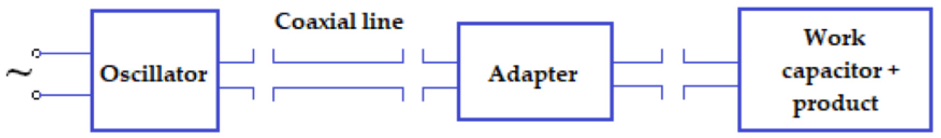
Figure 1 shows the block diagram of the installation used for processing the dielectric.
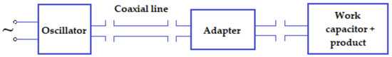
Figure 1.
Block diagram of the installation used for processing the dielectric.
Recently, more and more specialists, engineers, and scientists have focused their research on numerical analysis techniques dedicated to engineering problems. The great diversity of issues that the engineer must solve in order to effectively design a structure is suggestively reflected in the multitude of existing calculation methods. These methods have gradually developed over time in the context of existing relationships between the theoretical and practical aspects. These techniques are based on the approximate solution of an equation or sets of equations that describe the concrete problem.
Specialists in electrical engineering from our faculty who, over time, have conducted extensive research on the heating and drying of wood in the microwave field, have found that, as a result of the aforementioned process, a degradation of the wood could be observed. As a result, research was initiated on heating and drying wood in the radio frequency field, this procedure being applied to the wood processing industry. Thus, we built the heating and drying installation in RF, which works at the frequency of 13.56 MHz, analysing the coupling problems of electromagnetic field, thermal field, and mass.
The qualitative analysis of the quasi-stationary electromagnetic field used in radio frequency (RF) must take account of variations in dielectric parameters. Therefore, from among the sources considered, a selection was performed, based on the identification of [5,10,14,15,16,17,18,19,20,21,22]. Often, the finite element method is used as a numerical calculation method in order to determine the field in different applications. This method was devised long before the use of computers for engineering design. In 1968, an application of this method, aimed at solving an electrical problem, was mentioned in a paper. In the same year, in the field of civil engineering, the first book with the finite element method as its main subject was also printed. Since the 1970s, this method has been very well studied from the mathematical point of view and its implementation on the computer has been examined. Nowadays, there are many such specialised program packages designed for solving various problems [23,24,25,26,27].
The above-mentioned process was studied in the literature [5,6,10,20,23]. However, as the coupling of the three components, i.e., electromagnetic, thermal, and mass, has not been thoroughly researched, we set for ourselves the goal of paying in-depth attention to this coupling.
An important objective is the calculation of the impedance of the applicator in the presence of the load. This is absolutely indispensable for the tuning, optimisation, and optimal power transfer from the high frequency oscillator to the product. In cases of improper adaptation, unpleasant phenomena, such as the return of the high-frequency component in the tubes, may occur.
Note: throughout this entire paper, bold letters are used to denote vectors, for example, E, H, D, J, while the classic normal symbols are used for scalar quantities, for example, ε, γ, σ, ρ, V.
The abbreviations associated with the quantities referred to in this paper are as follows:
- E—intensity of the electric field;
- D—electric induction;
- J—density of the electric current;
- H—intensity of the magnetic field;
- V—electric potential;
- ε—electric permittivity;
- σ—electric conductivity;
- δ—losses angle.
2. The Mathematical Modelling of the Electromagnetic Field in Radio Frequency Heating
Radio frequency heating assumes the non-magnetic quasi-stationary regime of the electromagnetic field [7,28] where the time derivative of the magnetic induction is neglected. The law of electromagnetic induction takes the following form of electrostatics:
for any closed curve Γ in the computational domain Ω. The local form is:
rotE = 0
The validity of the electric potential theorem results from Equation (1) as follows:
where the integral is performed on any path from P0 to P, and P0 is a point with an arbitrarily fixed reference potential. The local form of the relation (3) is:
E = −grad V
The law of the magnetic circuit, written for a nonlinear environment, is:
whatever the surface SΓ ⊂ Ω, with border Γ. The local form is:
The law of the connection between the electric induction and the intensity of the electric field for homogeneous and non-dispersive material is:
D = εE
The law of conduction is:
J = σE
Linear isotropic media were assumed without permanent electric polarisation and without printed field.
Equations (2) and (6)–(8) can be considered like a system of four equations, with four unknown quantities: E, D, J, H.
It is also necessary to add the boundary conditions (BC), these being of the same type as those from the quasi-static fields [16,29]. This assumes that only the intensity of electric field and power density are to be taken into account, the magnetic component being neglected.
(α): on the surface S′ ∊ ∂Ω n the tangential component of E: Et = f is given;
(β): on the rest of the border S″ = ∂Ω − S′ the normal component of the total current density is given:
If the surface S′ is formed from n disjoint surfaces:
Then, the following are also given:
(γ): the total currents on (n − 1) surfaces named Si
or
(γ′): the voltages on (n − 1) curves on Ci from Ω, that connects one point from Si with another point from Sn:
Because the time derivative of electrical induction is present in Equation (6), it is necessary to know its initial value:
In order to solve the electromagnetic field equations, Theorem 1, Theorem 2, and Theorem 3 are used [17].
Theorem 1.
The system formed from Equations (2) and (6)–(8), with the initial condition (IC) and the boundary condition (BC), is verified by unique values of the E, D, and J fields.
Remark 1:
- The intensity of the magnetic field H cannot be uniquely determined, because only rotH is known.
- If the medium is perfectly insulating, then J = 0 and, from the relation (5), it follows that:Therefore, we obtain:divD = const. (in time)Knowing the value of divD = const. at the initial time, it follows that the quasi-steady state problem is, in fact, an electrostatics problem.
- Neglecting the time derivative of the magnetic induction, which defines the quasi-stationary regime, corresponds to the choice of a zero magnetic permeability [21].
2.1. The Equation in Scalar Potential
Replacing relation (4) in relations (7) and (8), and taking into account relation (5), it results that:
Applying div operator, the following is obtained:
The boundary conditions for the equation in V are obtained from (BC), which is presented above in the paper. From (α) condition and from relation (3), it follows that on each of the surfaces Si the variation of the potential V is given:
where P and P0 are points on the surface Si and the integration is made on any way from Si. On the surface S″, there is a relation of the derivative on the direction of the normal:
Choosing the condition (γ′) and taking into account relation (10), it follows that we have the value of the potential V on the entire surface S′ (we fix the zero value for the potential from an arbitrary point).
2.2. The Sinusoidal Regime
If all the magnitudes of the field in the quasi-stationary regime are sinusoidal functions of the same pulsation, we can use the complex images and, according to relations (3) ÷ (8), we obtain:
In relation (14), the complex permittivity is considered:
by which we take into account the losses in the dielectric. In practice, dielectric losses are described by:
The potential equation is:
where the complex conductivity also includes conduction losses:
The initial condition, which appears in the time domain problem, is replaced by the condition that the quantities are sinusoidal functions. The boundary conditions for the complex image of the potential are:
where results from relation (21) and condition (γ′). The classic Dirichlet and Neumann boundary conditions are recognised.
Theorem 2.
Equation (18), under the boundary conditions , has a unique solution.
Remark 2:
If the medium is insulating, then σ = 0, and, if simplifying with jω, relation (18) becomes:
2.3. Dielectric Losses
Warburg’s theorem states that the specific energy (volume density) that transforms from the electromagnetic form into heat is [30,31,32,33,34,35]:
As a result, the specific losses can be written:
where T is the period.
Using the images in the complex and the scalar product theorem, we have the following:
Using the complex permittivity expression (16), it follows that:
If conduction losses are also taken into account, then it follows:
Using the complex conductivity expression (19), it follows:
which includes both dielectric and conduction losses.
2.4. Finite Element Method
We propose to solve Equation (18) considering a quasi-electrostatic field. For Equation (20), we only replace σ with ε. The conditions (BCV) are met at the border.
Next, a Galerkin technique for solving Equation (20) is presented. We look for the solution of the equation in the set of potentials that verify the Dirichlet boundary condition (α). Let be linearly independent functions, called test functions, which have the zero Dirichlet boundary condition: = 0 on S′ [36,37,38,39,40,41,42]. We project Equation (20) on these functions:
We integrate by parts the left member from the relation above as follows:
taking into account the fact that the test functions are zero on S′ and substituting the Neumann boundary condition, the first term in the right-hand member becomes the following:
Instead of expression (27), we insert, taking into account relations (28) and (29), as follows:
whatever . Thus, Equation (18) and the Neumann boundary condition are verified.
In numerical procedures, is chosen as a function of a finite number N of parameters, choosing also N test functions as follows:
where is a known component that has the Dirichlet boundary condition and are given functions, linearly independent, that have the zero Dirichlet boundary condition (called shape functions). Substituting relation (31) into (30), we achieve the following:
The following system of equations is obtained:
where
2.5. Nodal Elements
The choice of test functions and shape functions is a topic for many works in the field of numerical analysis. A particularly efficient variant is to choose the shape functions equal to the test functions and, for both, to choose the nodal element of order 1. To make the context easier, we start with . We define on Ω a network of triangles, in which there are no nodes inside some sides (Figure 2).
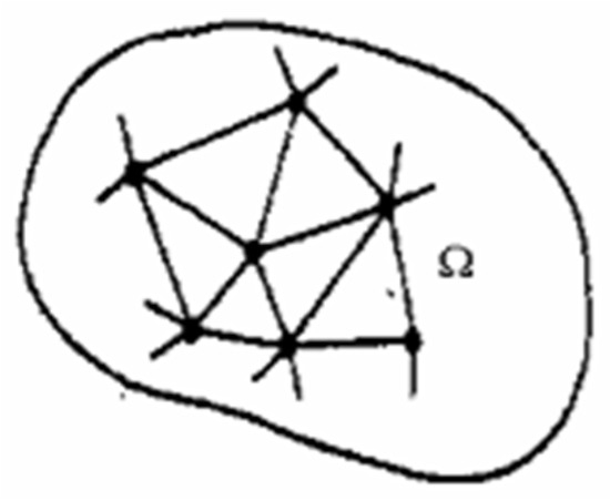
Figure 2.
The network of triangles.
The nodal element of order 1 of node k is a function with linear variation in each triangle, which has the value 1 in node k. In the rest of the nodes, its value is zero (Figure 3).
where
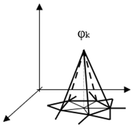
Figure 3.
Nodal element.
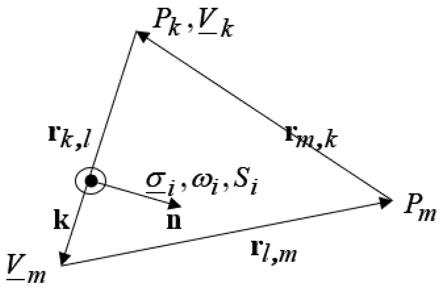
ωi is the domain that contains the node k (Figure 4), , and k is the versor of z axis.

Figure 4.
The domain that contains the node k.
Taking into account relations (36)–(38), relations (34) and (35) then become:
The potential can be expressed as a combination of nodal functions as follows:
where Pj are points on the Dirichlet border and ND is the number of these nodes.
The terms from relation (35) become the following:
where j ∈ {k} refers to the nodes on the Dirichlet frontier, neighbours of the node Pk, the expression being non-zero only if the node Pk is in the vicinity of the Dirichlet frontier.
- Observations
- In the case of 3D domains, we define a mesh of tetrahedra and have the following:whereis the index of the tetrahedron containing the node Pk, is the surface facing outwards, from the i tetrahedron, opposite the node Pk, and Vi is the volume of the i tetrahedron (Figure 5).
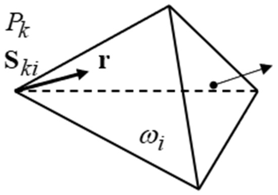 Figure 5. Tetrahedral element.
 - The matrix of system coefficients (39) is sparse non-zero elements on each line corresponding to the neighbouring nodes of the node that defines the line.
2.6. Load Capacity
It is known that, in radio frequency heating installations, the material to be heated is arranged in a condenser-type applicator. The capacitor electrodes are supplied with sinusoidal voltage through an electronic power circuit. In order to design the circuit, it is necessary to know the parameters of the circuit element equivalent to the load. In the simplest version, it is assumed that the load can be modelled by an ideal capacitor [43,44,45,46,47]. In reality, dielectric losses require the introduction of a resistor that can be connected in parallel if we also have conduction, or in series, if we only have electrical losses (Figure 6).
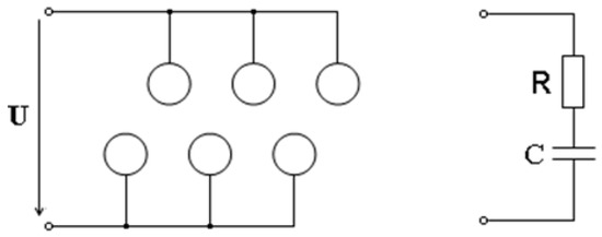
Figure 6.
The applicator.
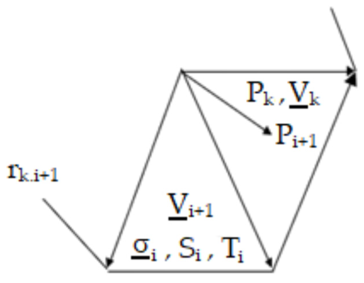
By solving the system (33), we obtain the potentials of the nodes in the finite element network and then the electric field intensity values in all triangles as a linear combination of the nodal elements.
For example, in the triangle ωi, (Figure 7), results as a linear combination of the gradients of the nodal elements of the peaks Pk, P1, and Pm of the triangle:

Figure 7.
Triangle ωi.
Taking account of relations (37) and (38), we obtain from Figure 6:
The value of the current density in the triangle ωi is:
The current on one side of the triangle results by integrating the expression (45). For example, on the side PkPl, we have:
where d is the depth on the OZ axis direction. After performing the mathematical calculation, it turns out that:
Summing the currents on all the sides that form the electrodes of one polarity, connected in parallel, we obtain the current and then the complex impedance:
If an RC series representation is desired for the load impedance, then:
If the medium is insulating, then Equation (20) is solved and the complex image of the electric induction is obtained by replacing in relation (45) with , being the complex permittivity of the triangle ωi:
the current density being:
The electric induction flux on the side PkPl is:
the current being:
The current of the electrodes is:
where is the electric flux of the electrodes. From relations (48) and (49) it follows:
Obviously, if , we obtain R = 0 and .
2.7. Thermal Field Diffusion
2.7.1. Thermal Field Equations, Mathematical Modelling of the Thermal Field during Radio Frequency Heating, and Stationary Regime
Let us consider the domain Ωθ with the border ∂Ωθ. The domain Ωθ is occupied by the dielectric with losses and is included in the calculation domain of the electromagnetic field Ω. The Fourier equation for the stationary regime of the thermal field is [48,49,50,51,52]:
where λ is the thermal conductivity and p is the volume density of the power that transforms from the electromagnetic form into heat, according to relations (24) and (26).
The border condition is:
where α is the heat transfer coefficient on the surface and Te is the temperature outside the domain Ωθ. Several times, Te = 0 can be taken. In such a case, we compare overtemperature to environment temperature. If, in relation (57), we have α = 0, we obtain homogeneous Neumann conditions, and, if λ = 0, the Dirichlet boundary condition results.
In order to solve the thermal field equations, Theorem 3, Theorem 4, Theorem 5, and Theorem 6 are used [17].
Theorem 3.
Equation (56) has a unique solution in the border condition (57).
Thermal Diffusion
The diffusion of the thermal field is described by the equation:
where c is the volumetric heat capacity. The boundary conditions (57) and the initial temperature condition are added to Equation (58): T(0) = Tin.
Theorem 4.
Equation (58) has a unique solution under the boundary condition (57) and with imposed initial condition.
2.7.2. The Finite Element Method and Stationary Regime
It is assumed that the boundary ∂Ωθ of the domain Ωθ consists of three surfaces SD, SN, and SF, where the following boundary conditions are fulfilled: Dirichlet T = Te, Neumann: , and, respectively, mixed The first two boundary conditions can be considered special cases of the mixed condition, when λ = 0 and, respectively, α = 0 (Section 2). From a technical point of view, the Neumann boundary condition appears on symmetry surfaces (field surfaces), being always zero. Unlike the case of the electromagnetic field, in the case of the stationary thermal field, the Ritz technique of numerical solution of Equation (56) will be presented.
The functional below has been considered:
whose minimum is sought in the set of functions that have the imposed Dirichlet boundary condition.
Theorem 5.
The solution of Equation (56), which checks the boundary conditions, minimises the functional (59) and, reciprocally, the minimum of the functional (59) is given by the (weak) solution of Equation (56), which also checks the Neumann and mixed boundary conditions.
Theorem 6.
The functional defined in relation (59) is strictly convex:
The Galerkin Procedure
The same problem can be treated by a Galerkin procedure, similar to Section 2.4. The temperature field is written in the form:
where φk are linearly independent functions with null Dirichlet boundary conditions, called shape functions, and TD is an arbitrary function that satisfies the Dirichlet boundary condition. Equation (56) is projected onto the linearly independent functions ψj, with zero Dirichlet boundary conditions, called test functions:
The left member is integrated by parts:
If the boundary conditions are taken into account, we obtain:
Replacing relation (64) by relation (63) and then by relation (62), it follows:
Taking account of relation (61), the system of equations results:
As shown in Section 2.4, the use of nodal elements is recommended.
Thermal diffusion is described by Equation (58):
The diffusion operator no longer enjoys the property of being positive definite and symmetric. For this reason, the numerical solution of Equation (67) is performed by the Galerkin procedure. The temperature is written in the following form:
Unlike the expression (61), in relation (68), the coefficients are functions of time. Equation (67) takes the following form:
2.7.3. Discretisation in the Time Domain
System (69) can also be written as follows:
where
The numerical solution of Equation (70) can be performed by the Crank–Nicholson method. Equation (70) is integrated over the time interval [ti, ti+1], of length Δti, as follows:
The integral in the time domain is approximated by:
where χ ∈ [0, 1] is a coefficient. In particular, we have the following situations:
- For χ = 0, the explicit Euler method;
- For χ = 1, the implicit Euler method;
- For χ = 1/2, the trapezoidal method.
Using relation (100), relation (99) becomes
where .
Relation (73) represents a system of equations with unknowns . The time step is corrected so that the norm of temperature variation becomes:
to keep within some imposed limits. If is obtained at time step , then the next time step is halved , and, if , and the next time step is doubled . In programs that couple electromagnetic fields and thermal and mass problems, the value of the free term at time depends on the value of moisture loss at time , which depends on tgδ and on the solution of the electromagnetic field problem, both of which depend on humidity. In turn, humidity depends on temperature through the rate of evaporation. For this reason, we choose , so in the right member of relation (73). There are no reasons to iteratively correct the value of .
2.8. Drying of Dielectrics in the Field of Radio Frequency
2.8.1. Model for Solving the Mass Problem
The evaporation of water from the wood mass takes place to a small extent inside the wood and to a large extent on the surface of the wood. Taking internal evaporation into account demands solving a complicated water diffusion problem, involving an inhomogeneous pressure field due to water vapour. The pronounced anisotropy of wood, due to the orientation of the wood fibre, makes a correct modelling of the diffusion problem impossible. In addition, during drying processes, the rapid emergence of water vapour inside the wood can lead to its destruction. For this reason, the maximum overtemperature inside the wood must be limited (below 70 °C). We can therefore neglect the evaporation from the inside and consider only evaporation from the surface of the wood. The rate of evaporation per surface unit depends on the difference between the temperature at the surface of the wood and the ambient temperature. It also depends on the degree of vapour saturation. As a result, the rate of decrease in the amount of water is as follows [53,54,55,56,57,58,59,60,61]:
where w is the rate of evaporation per surface unit, corresponding to a difference of 1 °C. In relation (74), we consider a linear dependence of the water evaporation rate in relation to the temperature difference. Solving the thermal problem at one time step and taking into account the Crank–Nicholson procedure, it follows from relation (74) that the water evaporated in one time step is
The humidity changes during a time step according to the relationship:
2.8.2. Coupling the Electromagnetic Field and Thermal and Mass Problems
Taking into account the latent heat of vaporisation, surface evaporation intervenes in the heat equation by increasing the heat transfer to the surface. Based on relation (74), it follows that the caloric power transferred to the surface for water vaporisation is [62,63,64,65,66,67]
where Λ is the latent heat of vaporisation.
In addition, considering the thermal transfer to the surface, given by boundary condition (57) from Section 2.7.1, we obtain the global boundary condition that also contains the surface evaporation as follows:
where
Relation (78) most simply models the coupling of the mass problem with the thermal problem.
The humidity defines the dielectric parameters (ε′, tgδ) needed to calculate the volume density of the losses. In the developed program, the correction of these parameters is performed by interpolation, using a table of values. For simplicity, only the effective value of the permittivity is considered in solving the electromagnetic field problem. In this case, the system matrix is real, diagonally dominant, and Hermitian. After obtaining the electric potential, the intensity of the electric field and the volume density of the losses is determined, taking into account ε′ and tgδ. In relation (24) (Section 2.3), it is determined by the relation that takes account of all the real material conditions as follows [17]:
3. Results
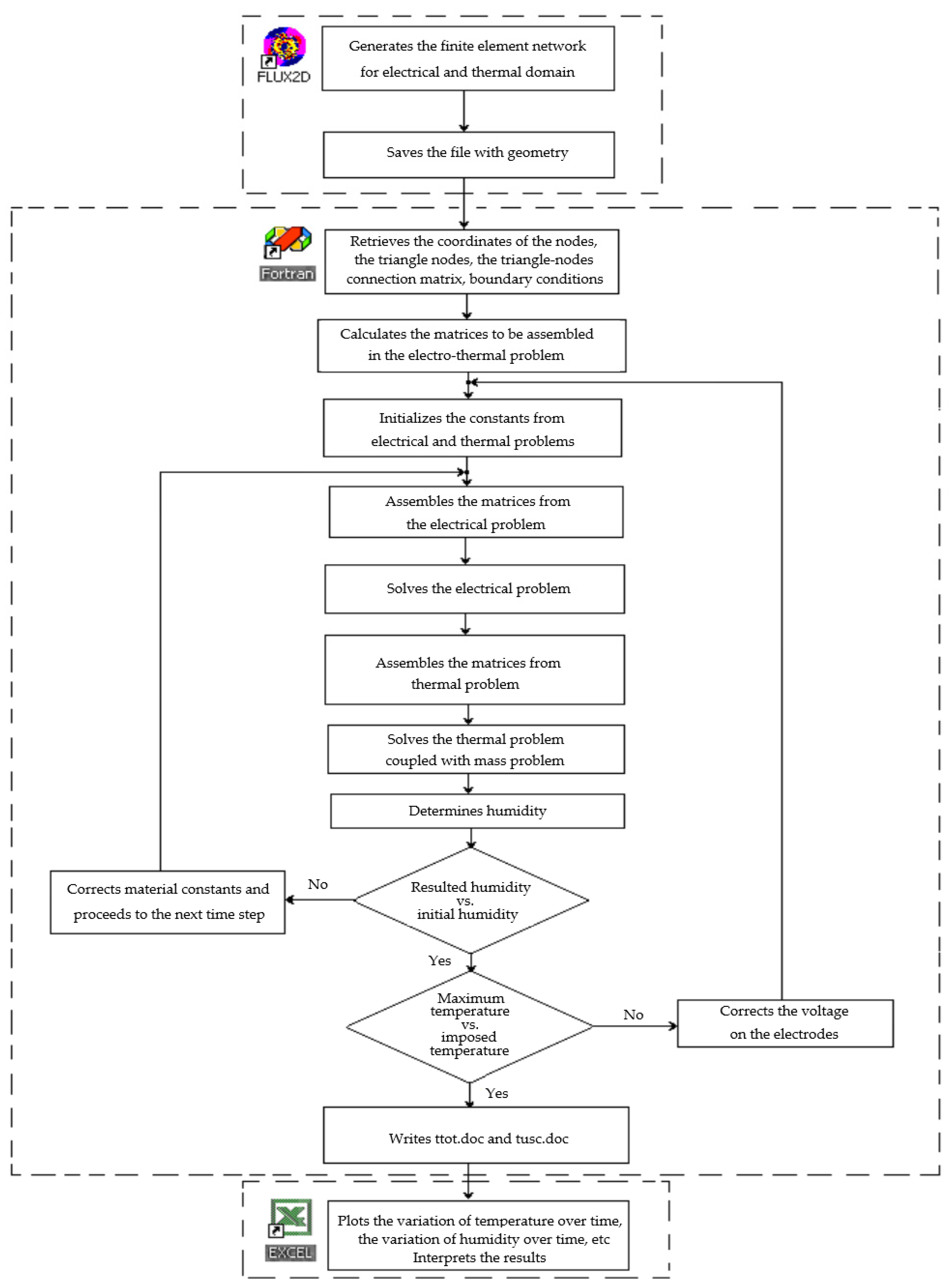
In drying technologies, it is essential to know the temperature field and, in order to avoid the destruction of the load and a correct modelling of the radio frequency, drying processes must take into account the percentage of water in the load. In this paper, a software package that allows numerical modelling of drying processes is developed [68,69]. This software couples the electromagnetic field, thermal problems, and mass problems based on the organisational chart presented in Figure 8.
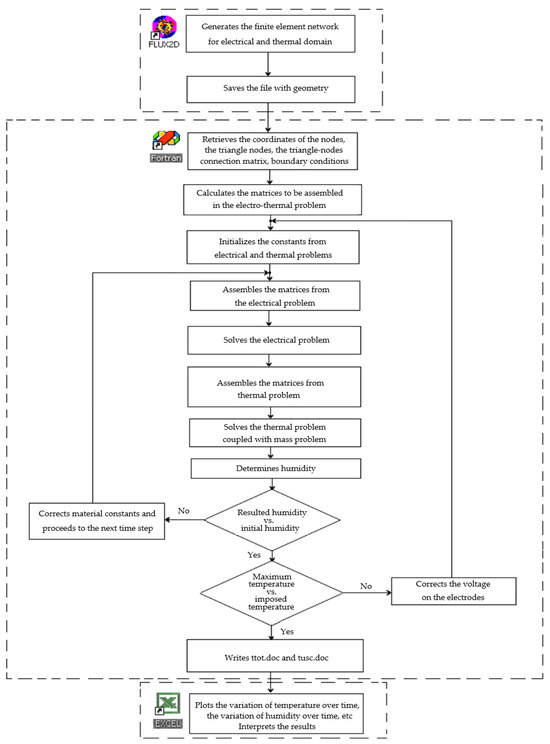
Figure 8.
Organisational chart illustrating the coupling problems.
This organisational chart includes the algorithms that are largely presented in the following steps:
Step 1. The meshes generated by FLUX-2D, the dielectric thermal module, are taken over. The developed program imports the mesh using alphanumeric characters whereby the locations of the data in the file created by the FLUX-2D mesh generator are recognised. The mesh created by FLUX-2D allocates six nodes per triangle (the vertices of the triangle and the midpoints of the sides). There are two possibilities as follows: either higher order shape functions are used or the four triangles that appear in each triangle are taken into account, using first order shape functions, with economy in the topological matrix.
Step 2. The program developed in this work takes only the nodes that describe the vertices of the triangles and the matrix. In addition, the coordinates of these nodes, the triangle nodes’ topological matrix, the types of media in the triangles, and the Dirichlet boundary conditions (the Neumann ones being free) are taken. Two of the media types have a special character—the external environment and the dielectric to be dried.
Step 3. The program renumbers the nodes and triangles and reconstructs the topological matrix, both for the electrical and the thermal programs.
Step 4. The matrices necessary to solve the electrical and thermal problems are built. The rarity of these matrices is taken into account, retaining only the non-zero elements and the address matrix. The construction of the matrices takes into account the change in material parameters due to humidity. The influence of temperature on these parameters can also be taken into account.
Step 5. The electrical problem is fixed. The Gauss–Seidel algorithm with super-relaxation is used. When initialising the iterative process, the final value from the previous time step is used.
Step 6. Specific losses are determined. Humidity is also taken into account.
Step 7. The thermal diffusion problem coupled with the mass problem is solved.
Step 8. Humidity is corrected. This is compared to the minimum imposed value and, if it has a higher value, the program returns to point 4. If the humidity is lower than the imposed one, it is considered that the load is dry.
Simulations were performed with the software developed by the authors, the organisational chart being presented in Figure 8 in the document. It can be added that, when running the program, it is considered that the dielectric is isotropic and it is assumed that vapourisation occurs only at the surface of the sample and that water diffuses instantly in the volume of the sample. In reality, there may be hot spots from which the water is vapourised, and the diffusion of the water does not take place instantaneously. Obviously, trying to take these aspects into account would be a failure, given that the properties of the load, from the point of view of water and vapour diffusion, cannot be controlled. This simplification results in the advantage that the humidity is constant throughout the volume of the mass and, as a result, the humidity dependence of the electrical and thermal parameters is greatly simplified. Going through the specialised literature [55,56], it is concluded that the maximum admissible overtemperature for wood-fibre processing must not exceed the value of approximately 70 °C. For this, the authors modify the initial program by introducing the possibility of limiting the maximum temperature by reducing the value of the supply voltage of the electrodes. Thus, to the initial steps in the algorithm, the following step is added.
If the maximum temperature in the load volume throughout the drying process exceeds an imposed maximum value Tmax_imposed or is lower than an imposed minimum value Tmin_imposed, the cycle from step 2 is resumed, modifying the boundary conditions by the factor: ; representing the initial value of the voltage applied to the electrodes. The overtemperature of 70 °C is chosen, which for an environment of 20 °C would correspond to a temperature of 90 °C. From here, results Tmax_imposed = 75 °C and Tmin_imposed = 65 °C.
The material properties for the fir-wood board are taken from the specialised literature [23,30,43,44,56,62,67].
- Observations
1. The program loads several result files containing at periodic time steps the following:
- The average value of the load temperature;
- The values of the temperature fields;
- The maximum and minimum values of the temperatures in the load and the points where they exit these extremes;
- Humidity;
- Drying time.
2. Equipotential and isotherms can be drawn at the time step where the average temperature is the highest.
3. Knowing the maximum values of the temperatures and the temperature differences (non-uniformity of the temperature field), the best solutions can be adopted for the drying equipment in the radio frequency field.
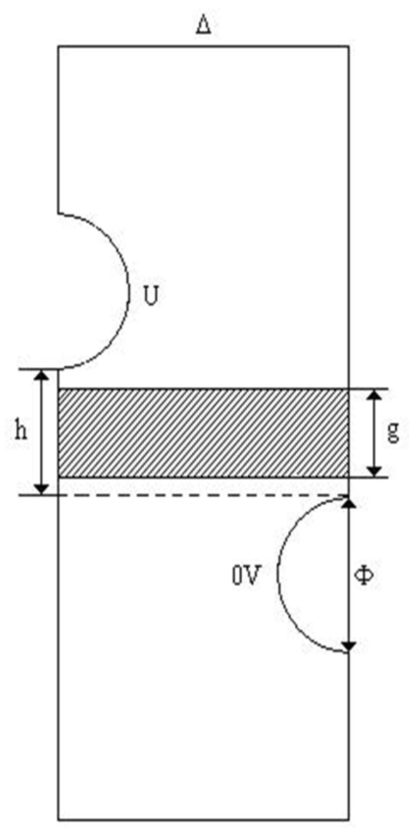
A geometry type is chosen, in which the dielectric material is placed between two consecutive electrodes (staggered-through geometry), according to Figure 9.

Figure 9.
Geometry of study domain.
We use a piece of fir-tree wooden board as the dielectric, taking into account its isotropic properties, and we admit that vapourisation occurs only at the load surface and water diffuses immediately in the load volume. This simplification leads to the advantages that the humidity is constant in the whole mass volume and, as a result, the humidity dependence of the electric and thermal parameters is greatly simplified. In addition, we impose that the overtemperature will not exceed 70 °C, the minimum temperature will be 65 °C, the maximum temperature will be 75 °C, and the initial humidity will be 50%. The material properties (ε’ and tgδ) are taken from the scientific literature [44,56,62]. The applied voltage on the superior electrode is U = 1100V and the working frequency is 13.56 MHz. The dimensions of the piece of wood are Δ = 1500 mm and g = 10 mm and the electrode diameter Φ = 10 mm.
We elaborate and develop a program written in Fortran, which solves the electromagnetic, thermal, and mass coupled problems. In order to fulfil the imposed limited final value accepted of 70 °C, after establishing the temperature field evolution for the voltage value of 1100 V, the supply voltage is corrected with coefficient , where Tmax represents the maximum temperature value in the load [70,71,72,73,74,75,76,77,78,79,80,81].
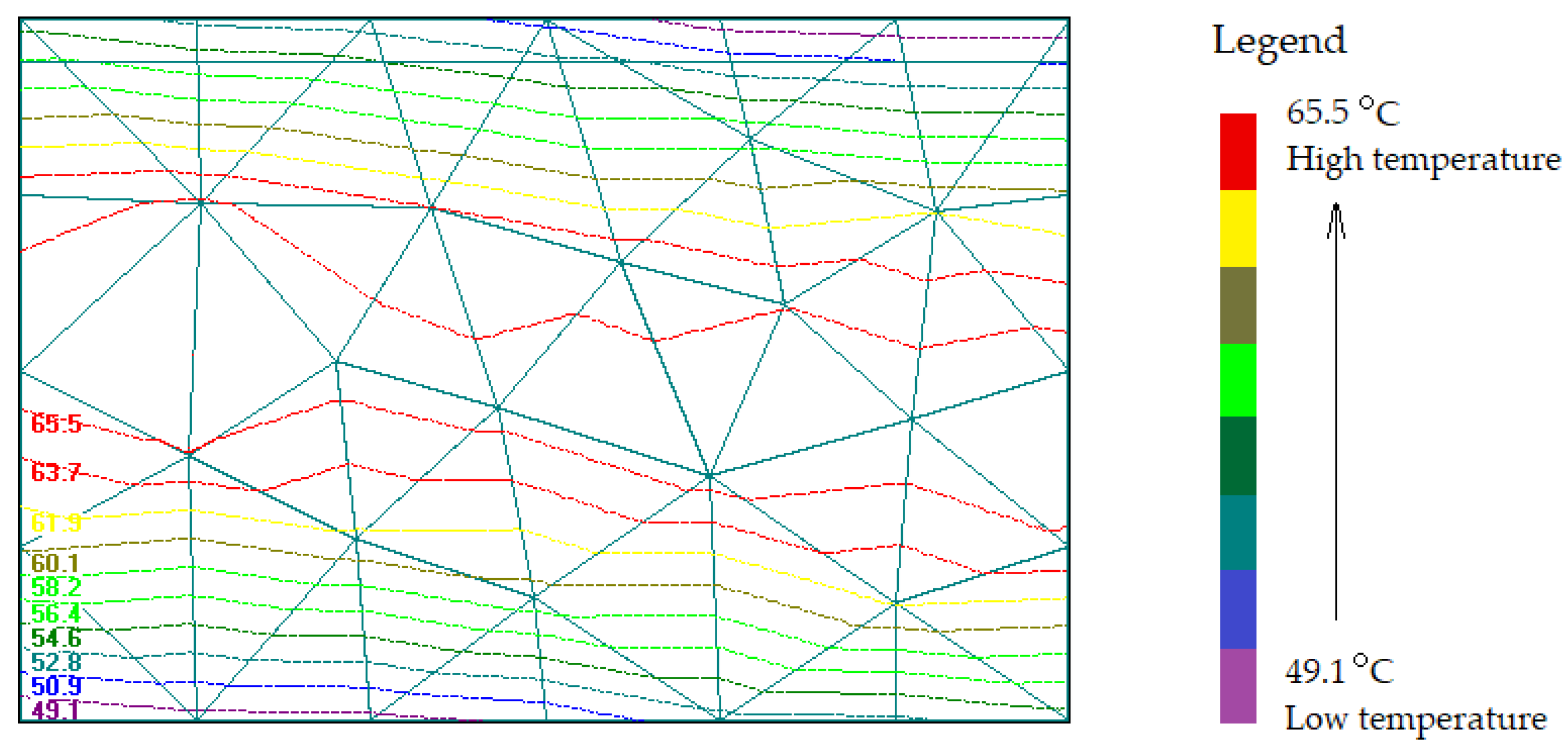
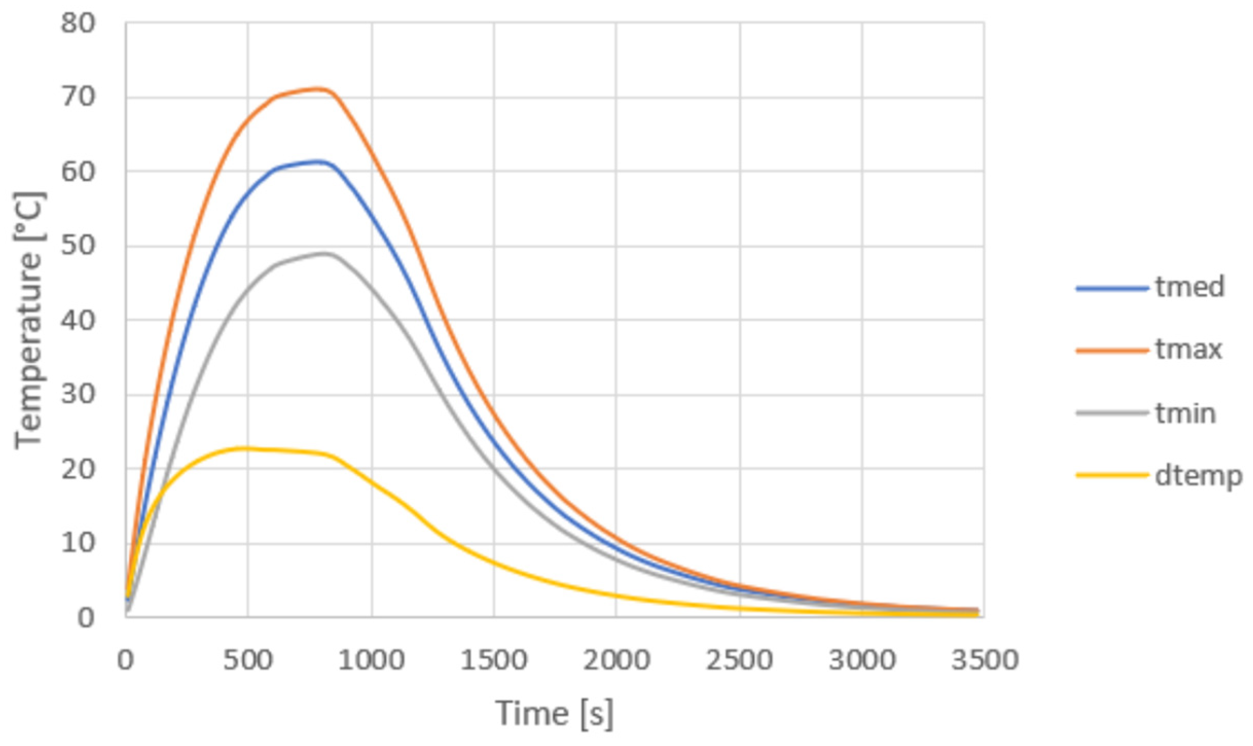
Figure 10 shows the equipotential in the field of calculations, while Figure 11 presents the meshes and isotherms in the plank. Figure 11 indicates the uniformity of temperature variation, showing therefore that the movement of load is not necessary. Figure 12 shows the optimised values of time temperature variation for the initial value of humidity (50%) (Figure 13).
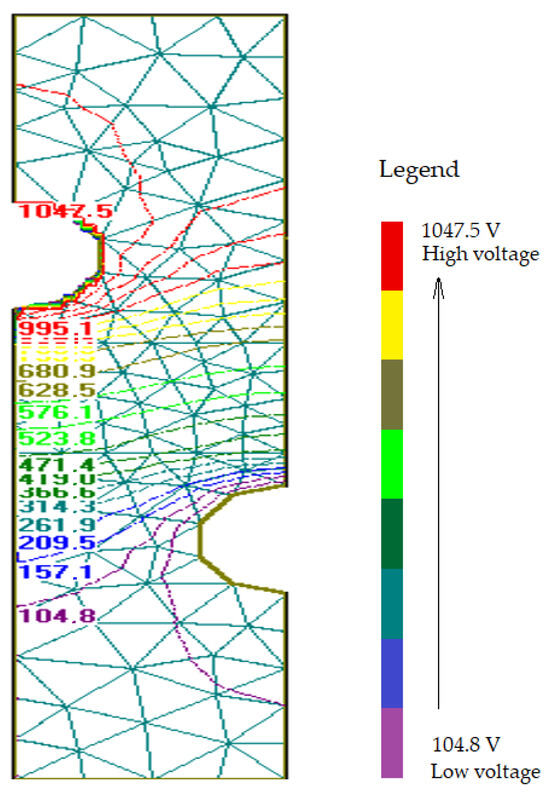
Figure 10.
Equipotential in the domain.
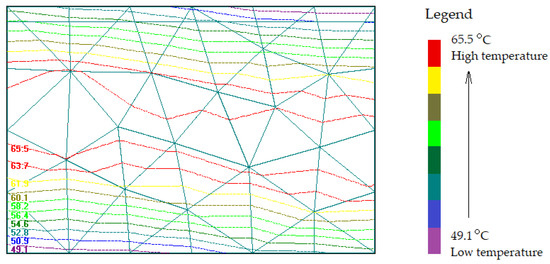
Figure 11.
Isotherms in the plank.
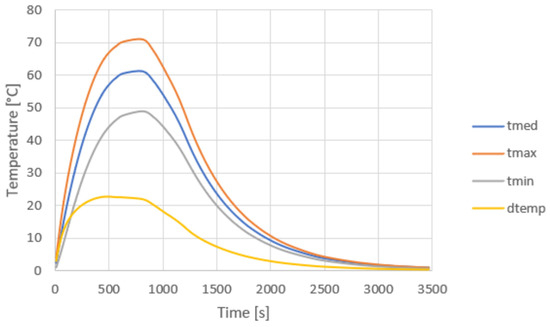
Figure 12.
Time–temperature variation in the dielectric in the drying process. tmed—medium temperature, tmax—maximum temperature, tmin—minimum temperature, dtemp—temperature difference.
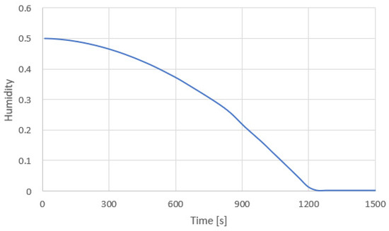
Figure 13.
Time–humidity variation in the dielectric in the drying process.
Final values of humidity are usually imposed in cases where wood processing is carried out in the industry. For example, in the case of furniture manufacturing technology, a final wood moisture value of about 12% is required, while 9% is required for instruments, etc. Figure 14 and Figure 15 show time–temperature and time–humidity variation for a 12% final value of humidity.
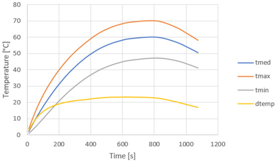
Figure 14.
Time–temperature variation for the 12% final value of humidity.
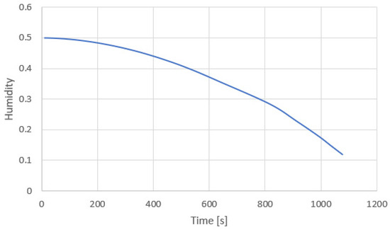
Figure 15.
Time–humidity variation for the 12% final value of humidity.
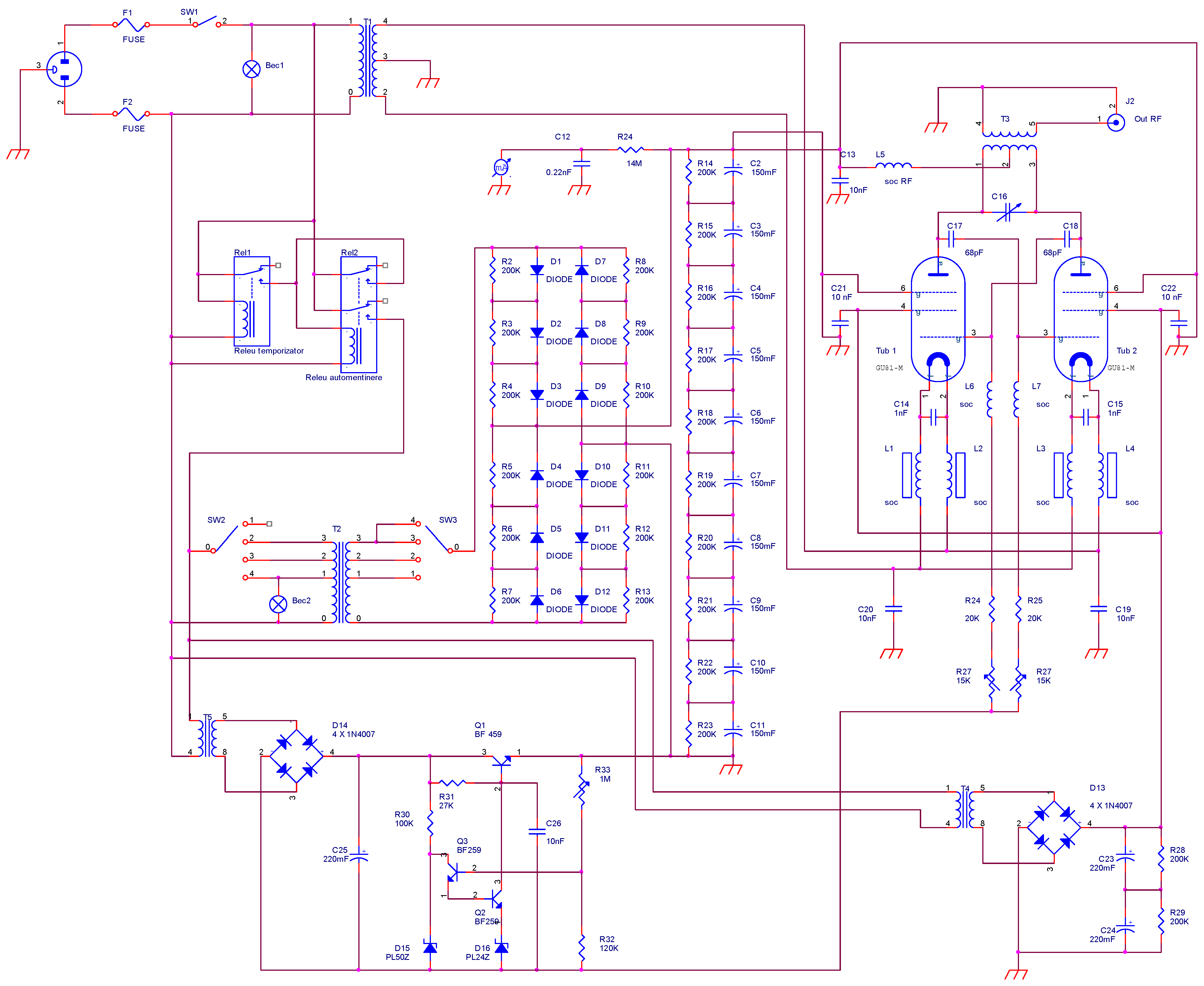
Figure 16 presents the electric and electronic diagram of the installation, made in OrCAD.
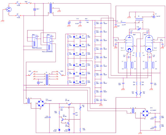
Figure 16.
Electric and electronic diagram of RF installation.
The RF drying installation presented in Figure 16 operates at 13.56 MHz frequency, with a useful RF power of about 1.3 kW. Pentode power tubes, GU81-M, are used. This choice is imposed for purchase reasons and to obtain sufficient processing power for dielectric processing. The oscillator is served by the filament supply block represented by transformer T1. This is a step-down transformer from 220 V to 12 V. The capacitors C19-C20 decouple the radio frequency voltage that may appear on the filament from ground. Also, for this purpose, four shock coils are provided—L1, L2, L3, and L4. The power supply block also includes the transformer T2—voltage booster 220–1430 V. After rectification and filtering thanks to the filter block, the voltage reaches the value of 2000 V. In order to be able to modify the emission power, the T2 transformer is provided both in the primary and in the secondary, with three sockets each. With the help of SW2 and SW3 switches, in different switching combinations, up to nine steps of anode voltage can be obtained. Bulbs B1 and B2 signal the presence of the supply voltage of transformers T1 and T2. Due to the need to apply the high anode voltage after the filaments of the tubes reach incandescence, a delay in supplying the transformer T2 is provided with the help of the timing block, composed of the time relay Rel1 and the self-maintaining relay Rel2. The anode voltage is applied through the shock coil L5 and decoupled through the capacitor C13 on the coupling transformer T3.
The presence of high voltage is signalled and measured with the help of the voltmeter. In order to protect the assembly against overload, fuses F1 and F2 are provided. The variable capacitor C16 is used for tuning the chosen frequency band. In order to negate grids G1 and G2, a 220–410 V voltage-raising transformer T3 is provided, with an adjustable stabiliser from the semi-adjustable R33 of negative voltage. The radio frequency voltage is collected from the secondary of the T3 transformer and transmitted to the applicator. For security reasons, the entire assembly is enclosed in an iron casing and placed on the protective earth. In addition, a thin wire mesh is arranged above the oscillator block as a shield.
Diagram Working
In the first stage, the level of the desired anodic voltage is established through switches SW2 and SW3. After energising the assembly by closing the switch SW1, it is fed transformer T1 and thus the filaments of tubes G1 and G2 are fed, a fact signalled by the lighting of bulb B1. After an interval of approximately 3 min, established by adjusting the timer relay Rel1, it feeds Rel2, which then feeds transformer T2, a fact signalled by the lighting of bulb B2. The negative voltage stabiliser is also powered, which then powers G1 and G2. Thus, the oscillator comes into operation, the frequency being adjusted by the capacitor C16 provided with access from the outside of the case. To change the anode voltage (and implicitly the power), SW2 is brought to zero, after which SW3 is actuated to the desired position. The values of the anode voltage steps are in the range 1030–1530 V. The connection between the oscillator and the applicator is made with a 50 ohm radio frequency cable for the optimal transfer of the radio frequency power.
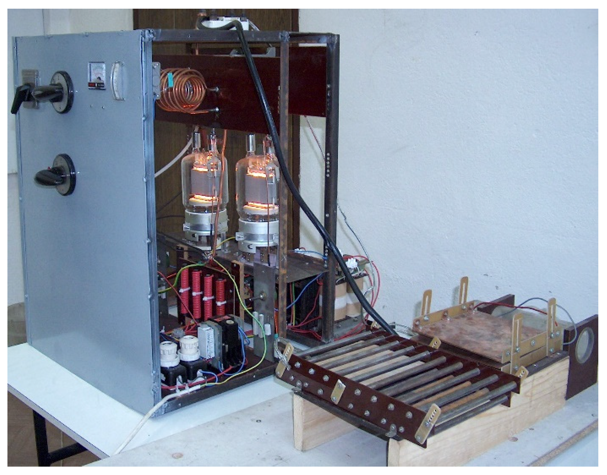
The prototype figure of the proposed model is presented in Figure 17. This prototype, used for the experimental part, consists of an electrothermal installation that contains the 13.56 MHz RF oscillator presented in Figure 16, coupled with a staggered-through field applicator, as shown in the figure. The software, with the organisational chart presented in Figure 8, is validated with measurements made with the built installation (Figure 17).

Figure 17.
The prototype installation.
The proposed model is original, as well as all the aspects and the phenomenon presented in this work. The authors contributed to the physical construction of the installation. Previous research, which consists of the study of wood heating by coupling the electromagnetic field with the thermal one, does not ensure very good accuracy of the simulated and experimental results. For this reason, this paper presents a simulation model that is built taking into account mass problems coupled with electromagnetic and thermal fields.
The “staggered-through field” is used as the applicator and the fir-tree wooden board is used as the dielectric. In order to simplify both the exploitation of the results and the comparison to the theoretical data, the thickness of the board is fixed at 10 mm, and the other dimensions are 1500 × 1800 mm. The geometric parameters of the applicator are chosen to be adjustable. The anode voltage is measured with the help of a digital multimetre, with a scale end of 5 kV.
To approximate the humidity, the piece of dry board is weighed with an electronic balance. The initial value is 107.8 g. The piece of timber is left submerged in a bowl of water for approximately 5 min and weighed again, resulting in a value of 117.3 g.
By repeating the operations specified above, the value of the initial humidity is approximated to 50%, corresponding to a wet board mass of about 163 g.
The drying experiment is started. To measure the temperature field, a point is fixed in the middle of the board on its surface, and a Micron infrared pyrometer is used. The geometric dimensions of the applicator are fixed.
To trace the temperature and humidity variation over time, the measurement is made intermittently by disconnecting the installation from the power supply.
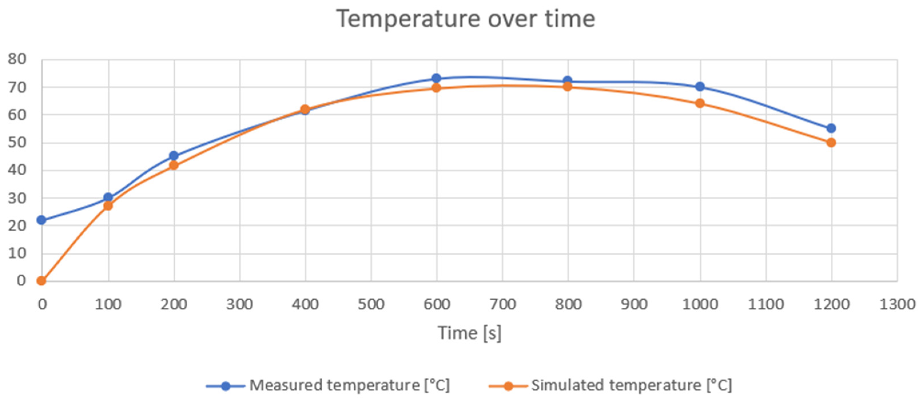
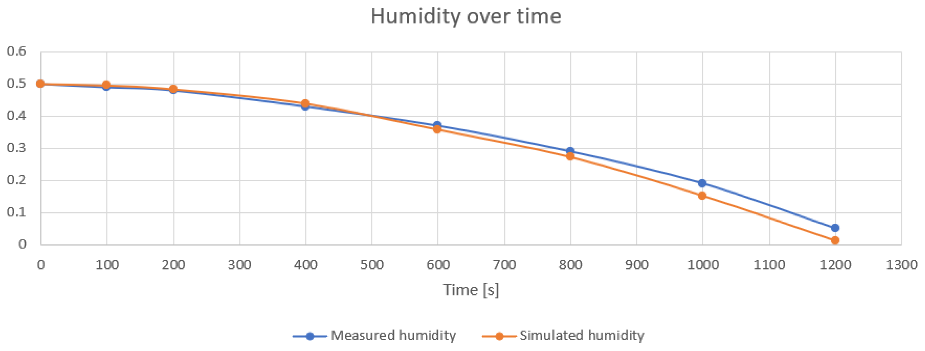
Figure 18 and Figure 19 present both simulated and experimental results for the temperature variation over time, respectively, for the humidity variation over time.

Figure 18.
Temperature variation over time.
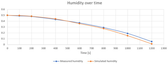
Figure 19.
Humidity variation over time.
In Figure 18, it can be observed that, for simulation, the initial temperature is 0 °C, because the software starts at 0 °C. The measurements start at 22 °C, the piece of wood being at the environmental temperature. Comparing the two sets of values, it can be seen that the measured values are slightly higher than the simulated values, the biggest difference being at the time point 1000 s, about 6 °C, and then the difference decreases slowly.
For humidity, both simulation and measurement start at 50% and, as much as the temperature increases, the humidity decreases. If the presence of water is taken into account, the temperature increases as long as the humidity keeps the values of permittivity and loss factor tgδ high. At a significant decrease in humidity, the support for the transformation of electromagnetic energy into caloric energy (water) is reduced, therefore the temperature decreases. Speaking about humidity, it can be observed in the above chart that the difference between simulated and measured values is small; the highest difference is about 3% at the time point 1200 s.
The maximum temperature measured reaches a value of around 73 °C, which is very close to the maximum temperature imposed in the software simulations. The voltage is set at 1100 V. The time until the initial weight is obtained and timed at about 21 min. The final temperature is around 60 °C. In the first phase of the drying process, it is possible to see light-coloured (dried) spots near the electrodes, after which they expand, respecting to a large extent the isotherms presented in Section 3. No visible degradation of the piece of board is found.
To emphasise the fact that the drying of wood in the RF field is superior to its drying in the microwave field, an experiment is carried out based on the microwave processing of the same dielectric. The installation is used with a microwave generator with a working frequency of 2.4 GHz and a variable power up to 1000 W. The plank dried in the microwave field shows visible signs of degradation.
4. Discussion
Most RF pulp processing applications require drying. In the absence of any program to be applied for the modelling of drying process, with the view of generating results, we made use of the Flux2D program, the dielectric thermal module, in order to create the geometry and discretisation of the study area. This was coupled with a program developed in Fortran, which models the electromagnetic, thermal field, and mass problem coupling, taking into account the variations of the dielectric properties at a frequency of 13.56 MHz.
Several runs were performed according to the geometric parameters of the study model (Figure 9) until acceptable dielectric temperature values were obtained, which were in accordance with the data in the specialised literature.
The final dielectric temperature and humidity values obtained by running the program were consistent with those obtained experimentally, with the latter using an infrared thermometer to measure the temperature and a scale to observe the loss of water from the dielectric. The time durations in the two cases were close.
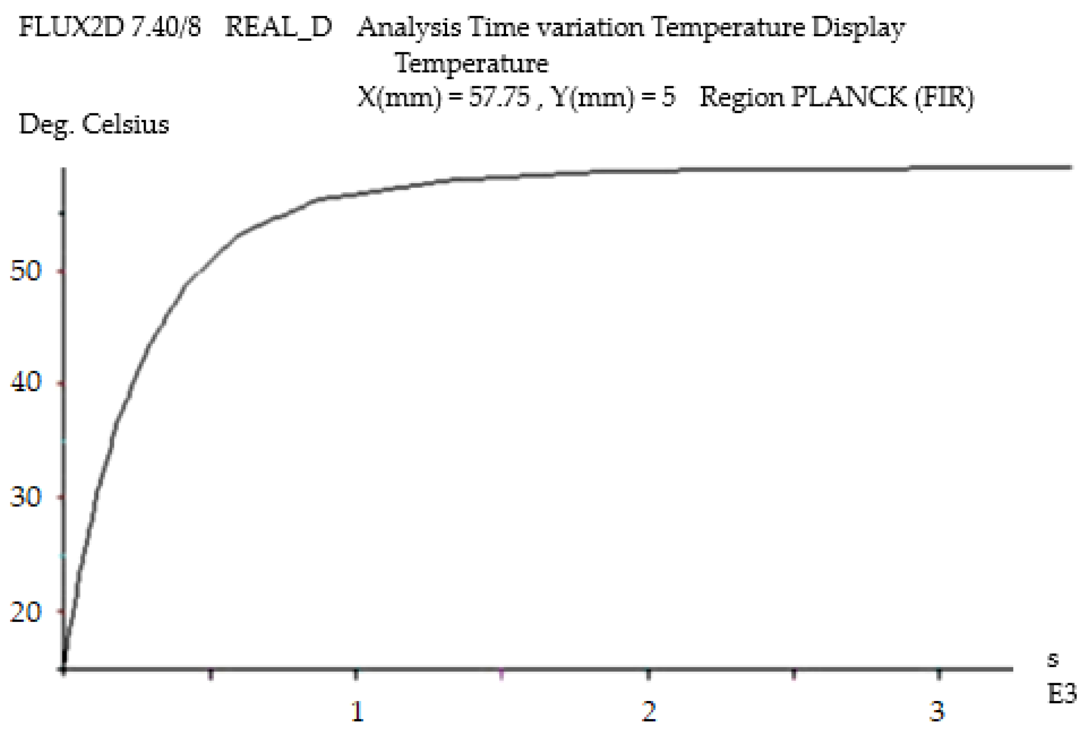
Figure 20 presents the time variation of temperature in the heating process of the dielectric. It can be observed that the temperature rose and stabilised at about 60 °C. In the drying process of the dielectric (Figure 12), the temperature reached a maximum and then decreased because the dielectric no longer absorbed heat.
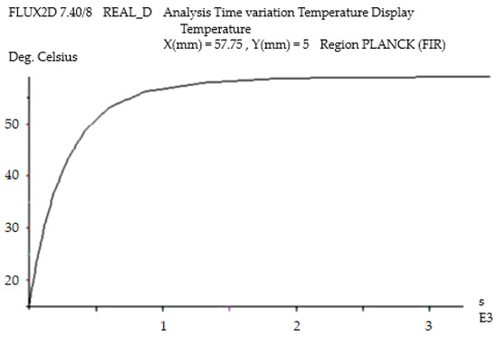
Figure 20.
Temperature–time variation in the heating process of the dielectric.
Future research must solve the coupling problems of the electromagnetic and thermal field together with mass problems, taking into account the movement of the dielectric between the electrodes.
5. Conclusions
The usual high-frequency techniques become very advantageous when considering the drying period with decreasing speed because, with the evaporation of water, the support of the transformation of electromagnetic energy into heat disappears, and the material cools without the need to control the radio frequency power.
The temperature of the dielectric increases as the size of the applicator decreases. Reducing the voltage applied to the electrodes represents an optimal measure since the qualities of the wood are not damaged in this way.
As regards temperature variation in the board, similar values have been identified when comparing experimental results to the data provided by the drying program. The theoretical processing time is about 100 s shorter. The differences are given by the efficiency of the installation, the final relative humidity as a comparison value, and the approximate values of the dielectric constants in the simulation part. The laboratory work leads to the completion of the mathematical model of the applicator, which aims in particular at maintaining the maximum allowed temperature by reducing the voltage on the electrodes.
Author Contributions
Conceptualisation, V.S., H.S. and D.S.; methodology, V.S., H.S. and D.S.; software, V.S. and D.S.; validation, V.S., H.S. and D.S.; formal analysis, V.S., H.S. and D.S.; investigation, V.S., H.S. and D.S.; resources, V.S. and D.S.; data curation, V.S., H.S. and D.S.; writing—original draft preparation, V.S., H.S. and D.S.; writing—review and editing, V.S. and D.S.; visualisation, V.S. and D.S.; supervision, V.S. and D.S. All authors have read and agreed to the published version of the manuscript.
Funding
This research received no external funding.
Data Availability Statement
The data will be made available by the authors on request.
Conflicts of Interest
The authors declare no conflicts of interest.
References
- Antti, A.L.; Torgovnikov, G. Microwave Heating of Wood. In Proceedings of the Microwave and High Frequency, International Conferences, Cambridge, UK, 17–21 September 1995; pp. E3.1–E3.4. [Google Scholar]
- Bergman, D.J. The Permitivity of a Simple Cubic Array of Identical Spheres. J. Phys. C Solid State Phys. 1979, 12, 4947. [Google Scholar] [CrossRef]
- Bossavit, A. Uniqueness of Solution of Maxwell Equations in the Loaded Microwave Oven, and How it May Fail to Hold. In Proceedings of the Microwave and High Frequency, International Conferences, Cambridge, UK, 17–21 September 1995; pp. A2.1–A2.4. [Google Scholar]
- Bouirdene, A. Les Fours Thermiques Micro-Ondes. Ph.D. Thesis, INP Toulouse, Toulouse, France, 1992. [Google Scholar]
- Fireţeanu, V. Procesarea Electromagnetică a Materialelor; Editura Politehnica Bucharest: Bucharest, Romania, 1995. [Google Scholar]
- Hobson, L. Basic principles of RF heating, Dielectric Heating Applications. In Proceedings of the Lecture Notes for a Short Course at EEB Staff Training College, Essendon, Australia, 9–13 September 1983. [Google Scholar]
- Leuca, T. Elemente de Teoria Câmpului Electromagnetic. Aplicaţii Utilizând Tehnici Informatice; Editura Universităţii din Oradea: Oradea, Romania, 2002. [Google Scholar]
- Lojewski, G. Microunde. Dispozitive şi Circuite; Editura Teora: Bucharest, Romania, 1996. [Google Scholar]
- Maghiar, T.; Leuca, T.; Bondor, K.; Silaghi, M.; Silaghi, H. Electrotehnică; Editura Universităţii din Oradea: Oradea, Romania, 1999. [Google Scholar]
- Roussy, G.; Pearce, J.A. Foundations and Industrial Applications of Microwave and Radio Frequency Fields. Physical and Chemical Process; John Wiley & Sons Ltd.: Hoboken, NJ, USA, 1995. [Google Scholar]
- Simion, E.; Maghiar, T. Electrotehnică; Editura Didactică şi Pedagogică: Bucharest, Romania, 1981. [Google Scholar]
- Şora, C. Bazele Electrotehnicii; Editura Didactică şi Pedagogică: Bucharest, Romania, 1982. [Google Scholar]
- Wei, J.; Hawley, M.; Asmussen, J. Microwave Power Absorption Model for Composite Processing in a Tunably Resonant Cavity. J. Microw. Power Electromagn. Energy 1993, 28, 234–246. [Google Scholar]
- Bocchi, W.; Grattieri, C. Michelangeli, Numerical Analysis of Electromagnetic Heating: Application to Dielectric Materials. In Proceedings of the International Seminar on Heating by Internal Sources, Padua, Italy, 11–14 September 2001; pp. 301–308. [Google Scholar]
- Brebbia, C.A. Boundary Elements X, Vol.2 Heat Transfer, Fluid Flow and Electrical Applications; Computational Mechanics Publications: Southampton, UK, 1988. [Google Scholar]
- Hănţilă, F.I. Observaţii Asupra Metodei Elementului Finit, Sesiunea de Comunicări Tehnico-Ştiinţifice, I.P.B; Faculty of Electrical Engineering: Bucharest, Romania, 1981; pp. 145–151. [Google Scholar]
- Hănţilă, F.I.; Demeter, E. Rezolvarea Numerică a Problemelor de Câmp Electromagnetic; Research Institute for Electric Machines; Ari Press: Bucharest, Romania, 1995. [Google Scholar]
- Leuca, T.; Bandici, L.; Molnar, C.; Nagy, A. Contributions Regarding the Electric Field Computation in Microwave Owens. In Proceedings of the International Conference RJJSAEM Felix SPA, Oradea, Romania, 11–15 September 2001; pp. 118–124. [Google Scholar]
- Leuca, T.; Bandici, L.; Molnar, C. The Numerical Modeling of Microwave Heating Problems. In Proceedings of the 27th Congress of the Romanian-American Academy of Science and Art and the International Book Fair, 10th Edition, Bucharest, Romania, 26 May 2002; pp. 720–724. [Google Scholar]
- Metaxas, A.C. The use of FE Modelling in RF and Microwave Heating. In Proceedings of the International Seminar on Heating by Internal Sources, Padua, Italy, 11–14 September 2001; pp. 319–328. [Google Scholar]
- Mocanu, C.I. Teoria Câmpului Electromagnetic; Editura Didactică şi Pedagogică: Bucharest, Romania, 1981. [Google Scholar]
- Orfeuil, M. Electric Process Heating; Edition Dunod: Paris, France, 1982; Volume II. [Google Scholar]
- Bialod, M.M.; Marchand, C. La Conception des Installations Industrielles de Chauffage Diélectriques par Haute Frequence et Micro-Ondes, Méthode, Technolojique, Exemples; Electricité de France, Direction des Etudes et Recherches: Paris, France, 1990. [Google Scholar]
- Zhao, H.; Turner, I.W. An Analysis of the Finite-Difference Time-Domain Method for Modeling the Microwave Heating of Dielectric Materials Within a Three-Dimensional Cavity System. J. Microw. Power Electromagn. Energy 1996, 31, 199–214. [Google Scholar] [CrossRef]
- Webb, J.P.; Maile, G.; Ferrari, R. Finite Element Solution of Three-Dimensional Electromagnetic Problems. IEEE Proc. H Microw. Opt. Antennas 1983, 130, 153–159. [Google Scholar] [CrossRef]
- Flux2D, Version 7.1; CAD Package for Electromagnetic and Thermal Analysis using Finite Elements, User’s Guide; CEDRAT: Massy, France, 1994.
- MacGfem. Gfem Documentation Plan; Numerica: Clamart, France, 1988. [Google Scholar]
- Boudrand, H. Introduction au Calcul Electromagnetique des Structures Guidantes; Institut National Polytechnique de Toulouse, ENSEEIHT: Toulouse, France, 1996. [Google Scholar]
- Bandici, L. Modelarea Numerică a Câmpurilor Electromagnetic şi Termic din Instalaţiile Electrotermice cu Microunde. Ph.D. Thesis, University of Oradea, Oradea, Romania, 2003. [Google Scholar]
- Anderson, J.C. Dielectriques; Edition Durand: Paris, France, 1996. [Google Scholar]
- Creţ, R. Contribuţii la Studiul Dielectricilor Neomogeni. Ph.D. Thesis, Technical University of Cluj Napoca, Cluj-Napoca, Romania, 2003. [Google Scholar]
- Helerea, E.; Tiganea, D.; Stanulet, D. Materiale Electrotehnice; Lithography of University of Braşov: Braşov, Romania, 1984. [Google Scholar]
- Leuca, T.; Molnar, C.; Bandici, L.; Nagy, A. Dielectric Materials Properties. Behaviour in the Microwave Field. In Proceedings of the 9th International IGTE Symposium, Graz, Austria, 11–14 September 2000; pp. 413–416. [Google Scholar]
- Nicula, A.; Puşkaş, F. Dielectrici şi Feroelectrici; Editura Scrisul Românesc: Craiova, Romania, 1982. [Google Scholar]
- Robert, P. Matériaux de L’électrotechnique; Presses Polytechniques Romandes: Laussannes, Switzerland, 1989. [Google Scholar]
- Maghiar, T.; Leuca, T. Carmen Molnar, Livia Bandici, The use of finite element in microwave heating. In Proceedings of the Progress in Electromagnetic Research Symposium, Pisa, Italy, 28–31 March 2004; pp. 321–324. [Google Scholar]
- Molnar, C. Contribuţii Privind Modelarea Numerică a Fenomenelor Electromagnetice din Instalaţiile Electrotermice cu Microunde. Ph.D. Thesis, University of Oradea, Oradea, Romania, 2004. [Google Scholar]
- Pichon, L. Finite element analysis of bounded and unbounded electromagnetic wave problems. In Proceedings of the IEE Colloquim on High Frequency Electromagnetic Modelling Techniques, London, UK, 30 March 1995. [Google Scholar]
- Silaghi, M.; Silaghi, H. Tehnologii cu Microunde. Tehnici Informatice; Editura Treira: Oradea, Romania, 2001. [Google Scholar]
- Spoială, D. Numerical modeling of electro-thermal field used for heating spherical dielectric pieces. In Proceedings of the 5th International Conference on Renewable Sources and Environmental Electro-Technologies, Stâna de Vale, Romania, 27 May 2004. [Google Scholar]
- Spoială, D.; Leuca, T. Numerical modelling of electromagnetic and thermal field in wood heating. In Applicator Optimization, Heating by Electromagnetic Sources; Session EF: Padua, Italy, 2004. [Google Scholar]
- Spoială, D.; Leuca, T. Numerical modeling of RF heating spherical rubber pieces. In Applicator Optimization; Simpozionul Naţional de Electrotehnică Teoretică: Bucharest, Romania, 2004. [Google Scholar]
- Bouirdene, A.; Lefeuvre, S. Measurement of thermal and dielectric parameters as function of temperature. In Proceedings of the International Conference, Arnhem, The Netherlands, 26–29 September 1989. [Google Scholar]
- Frandoş, S. Procesarea Materialelor Dielectrice în Câmpuri Electromagnetice de Radio-Frecvenţă şi în Microunde. Ph.D. Thesis, Universitatea Politehnica din București, Bucharest, Romania, 2003. [Google Scholar]
- Keam, R.; Green, A.D. Measurement of Complex Dielectric Permittivity at Microwave Frequencies a Cylindrical Cavity. Electron. Lett. 1995, 31, 212–214. [Google Scholar] [CrossRef]
- Spoiala, D. Modelarea Câmpului Electromagnetic în Regim Cvasistaționar la Înaltă Frecvență. Aplicații la Proiectarea Instalațiilor Electrotermice de Radiofrecvență; Editura Universitatii of Oradea: Oradea, Romania, 2005. [Google Scholar]
- Woode, R.A.; Ivanov, E.N.; Tobar, M.E.; Blair, D.G. Measurement of dielectric loss tangent of alumina at microwave frequencies and room temperature. Electron. Lett. 1994, 30, 2120–2122. [Google Scholar] [CrossRef]
- Jones, P. EA Technology—The Industrial Applications of RF and Microwave Heating, Short Course, Microwave and High Frequency Heating; Capenhurst: Chester, UK, 1995. [Google Scholar]
- Leuca, T.; Maghiar, T.; Silaghi, M.A.; Spoială, D.S. Roman, Numerical analysis of electromagnetic and thermal field in radio frequency applicators. In Proceedings of the 3rd Japan Romania Joint Seminar on Applied Electromagnetics and Mechanical Systems, Felix Spa, Oradea, Romania, 11–15 September 2001; pp. 124–129. [Google Scholar]
- Maghiar, T.; Şoproni, D. Tehnica Încălzirii cu Microunde; Editura Universitatii din Oradea: Oradea, Romania, 2003. [Google Scholar]
- Metaxas, A.C.; Meredith, R.J. Industrial Microwave Heating; Peter Peregrinus LTD (IEE): London, UK, 1983. [Google Scholar]
- Thuéry, J. Les Micro-Ondes et Leur Effets sur la Matiér; Deuxième Edition; Technique et Documentation: Lavoisier, France, 1989. [Google Scholar]
- Avramidis, S. Radio Frequency/Vacumm Drying of Wood. In Proceedings of the International Conference of COST Action El 5 Wood Drying, Ediburgh, Scotland, UK, 13–14 October 1999. [Google Scholar]
- Avramidis, S.; Zwick, R. Exploratory radio frequency/vacumm drying of three D.C. coastal softwoods. Forest Prod. J. 1992, 48, 17–24. [Google Scholar]
- Avramidis, S.; Zwick, R. Comercial scale RF/V drying of softwood timber. Part I, II. Drying characteristics and timber quality. Forest Prod. J. 1996, 46, 27–36. [Google Scholar]
- Beldeanu, E. Produse Forestiere şi Studiul Lemnului; Editura Universitatii Tehnice din Braşov: Braşov, Romania, 2001. [Google Scholar]
- Clemens, M.J. Experience on Radio Frequency dryer for textil fabric webs. In Proceedings of the International Conference, Arhem, The Netherlands, 26–29 September 1989. [Google Scholar]
- Leuca, T.; Spoială, D.S. Roman, Electrotermal installation for processing of the high-frequency electromagnetic field. In Application Consisting of the Wood-Dust Drying in Radio Frequency, Annals of University of Oradea, Romania; Electrotechnical Fascicola; University of Oradea: Oradea, Romania, 2002. [Google Scholar]
- Resch, H.; Gautsch, E. Drying of Lumber in Vacuum using Dielectric Heating, Cost Action E 15, Advances in drying of wood, (1999–2003). Holzforschung und Holzverwertung 2000, 52, 105–108. [Google Scholar]
- Resch, H. High Frequency Heating Continued with Vacuum Drying of Wood. In Proceedings of the 8th International IUFR Wood Drying Conference, Brasov, Romania, 24–29 August 2003; pp. 127–132. [Google Scholar]
- USDA. AirDrying of Lumber; United States Department of Agriculture, Forest Service, Forest Products Laboratory: Washington DC, USA, 1999.
- Leuca, T.; Spoială, D. St. Roman, The Electromagnetic Field Distribution in a Radio Frequency Applicator Used for Poliester Bands Heating; Heating by Internal Sources; Session EF: Padova, Italy, 2001; pp. 365–370. [Google Scholar]
- Simpson, W.; TenWolde, A. Physical Properties and Moisture Relations of Wood, Chapter 3. In Wood Handbook; Forest Products Laboratory, US Department of Agriculture: Madison, WI, USA, 1999. [Google Scholar]
- Torgovnikov, G.I. Dielectric Properties of Wood and Wood Based Materials; Springer: Berlin/Heidelberg, Germany, 1993. [Google Scholar]
- Zhou, B.; Avramidis, S. On the Loss Factor of Wood during Radio Frequency Heating. In Wood Science and Technology; Springer: Berlin/Heidelberg, Germany, 1999; pp. 299–310. [Google Scholar]
- Wood Use. U.S. Competitiveness and Technology; Congres of the United States, Office of Technology Assesment: Washington, DC, USA, 1984; Volume II.
- Wood Handbook, Wood as an Engineering Material; Forest Products Laboratory, U.S. Department of Agriculture: Washington, DC, USA, 1999.
- Grigoraş, G.; Chiruţă, C. Culegere de Probleme de Programare în Limbaj FORTRAN; Lithography of Al. I. Cuza University Iaşi: Iași, Romania, 1977. [Google Scholar]
- Flux2D, Version 7.30; CAD Package for Electromagnetic and Thermal Analysis Using Finite Elements, Dielectrothermal application User’s Guide; CEDRAT: Massy, France, 1998.
- Leuca, T.; Spoială, D. Particularities of the Dielectric Heating in RF; Applicator Optimization; ACTA Academy of Technical Sciences of Romania (Tehnical University of Cluj-Napoca): Cluj-Napoca, Romania, 2006; Volume 47, pp. 153–157. ISSN 1841-3323. [Google Scholar]
- Teodor, L.; Dragoş, S.; Livia, B.; Alexandra, P.P.; Ilie, S. The numerical analysis of electromagnetic and thermal field at the processing of semi-manufactured wood in a RF field. J. Electr. Electron. Eng. 2010, 3, 103–106. [Google Scholar]
- Marcela, L.B.; Dragos, S. Numerical Modeling of The Electromagnetic Field Of Pine Plank In Radio Frequency Heating. J. Electr. Electron. Eng. 2012, 5, 79–82. [Google Scholar]
- Marcela, L.B.; Teodor, L.; Dragos, S. Aspects concerning the heating/drying of oak planks in a radiofrequency field. J. Electr. Electron. Eng. 2013, 6, 59–62. [Google Scholar]
- Dragoș, S.; Constantin, G.N. Aspects regarding the dielectric heating of small wood boards in radio-frequency. J. Electr. Electron. Eng. 2017, 10, 51–54. [Google Scholar]
- Vikberg, T.; Sandberg, D.; Elustondo, D. High Frequency Heating in Solid Wood Modification. In Proceedings of the Seventh European Conference on Wood Modification (ECWM7), Lisbon, Portugal, 10–11 March 2014; pp. 113–114. [Google Scholar]
- Ravindra, V. Gadhave, Radio Frequency Gluing Technique for Wood-to-Wood Bonding: Review. Open J. Polym. Chem. 2023, 13, 15–26. Available online: https://www.scirp.org/journal/ojpchem (accessed on 25 December 2023).
- Tubajika, K.M.; Jonawiak, J.J.; Mack, R.; Hoover, K. Efficacy of radio frequency treatment and its potential for control of sapstain and wood decay fungi on red oak, poplar, and southern yellow pine wood species. J. Wood Sci. 2007, 53, 258–263. [Google Scholar] [CrossRef]
- Leuca, T.; Coman, S.; Trip, N.D.; Bandici, L.; Codrean, M.; Perte, M. Neural Network Modeling of a Drying Process in Radio Frequency Field. In Proceedings of the 15th International Conference on Engineering of Modern Electric Systems, Oradea, Romania, 13–14 June 2019. [Google Scholar]
- Janowiak, J.J.; Szymona, K.S.; Dubey, M.K.; Mack, R.; Hoover, K. Improved Radio-Frequency Heating through Application of Wool Insulation during Phytosanitary Treatment of Wood Packaging Material of Low Moisture Content. For. Prod. J. 2022, 72, 98–104. [Google Scholar] [CrossRef]
- Dubey, M.K.; Janowiak, J.; Mack, R.; Elder, P.; Hoover, K. Comparative study of radio-frequency and microwave heating for phytosanitary treatment of wood. Eur. J. Wood Wood Prod. 2016, 74, 491–500. [Google Scholar] [CrossRef]
- Leuca, T.; Laza, M.; Bandici, L.; Cheregi, G. George Marian Vasilescu, Oana Mihaela Drosu, FEM-BEM Analysis of Radio Frequency Drying of a Moving Wooden Piece. Revue Roumaine de Sciences Technique—Électrotechnique et Énergetique 2014, 59, 361–370. [Google Scholar]


Disclaimer/Publisher’s Note: The statements, opinions and data contained in all publications are solely those of the individual author(s) and contributor(s) and not of MDPI and/or the editor(s). MDPI and/or the editor(s) disclaim responsibility for any injury to people or property resulting from any ideas, methods, instructions or products referred to in the content. |
© 2024 by the authors. Licensee MDPI, Basel, Switzerland. This article is an open access article distributed under the terms and conditions of the Creative Commons Attribution (CC BY) license (https://creativecommons.org/licenses/by/4.0/).