Asymptotic Form of the Covariance Matrix of Likelihood-Based Estimator in Multidimensional Linear System Model for the Case of Infinity Number of Nuisance Parameters

Abstract

This article is devoted to the synthesis and analysis of the quality of the statistical estimate of parameters of a multidimensional linear system (MLS) with one input and m outputs. A nontrivial case is investigated when the one-dimensional input signal of MLS is a deterministic process, the values of which are unknown nuisance parameters. The estimate is based only on observations of MLS output signals distorted by random Gaussian stationary $m$-dimensional noise with a known spectrum. It is assumed that the likelihood function of observations of the output signals of MLS satisfies the conditions of local asymptotic normality. The $\sqrt{n}$-consistency of the estimate is established. Under the assumption of asymptotic normality of an objective function, the limiting covariance matrix of the estimate is calculated for case where the number of observations tends to infinity.

1. Introduction

The model of observations of the output MLS signals, which is used to estimate MLS parameters, has the form:

$$z_{u,t}=y_{u,t}+{\xi }_t, y_{u,t}={\displaystyle \sum _{\tau =0}^{\infty }{h}_{t-\tau }\left(u\right)s_t}, t\in \overline{1,n},$$

where $z_{u,t}\in {ℝ}^m$, $t\in \overline{1,n}$, and $n>q$ are observations of the output MLS signals $y_{u,t}$ distorted by the noise ${\xi }_t$; $h_{\tau }\left(u\right)=\left(h_{k,\tau }\left(u\right), k\in \overline{1,m}\right), \tau \in \overline{0,\infty }$ is the impulse response of MLS; and $s_t\in {ℝ}^1$, $t\in \mathbb{Z}$ is the input signal of MLS, whose values are unknown nuisance parameters.

The value $u$ of the parameter of observations $z_{u,t}$ is unknown and belongs to the open set $\tilde{U}$ of the $q$-dimensional vector space $u\in \tilde{U}\subset {ℝ}^q$. The functions $h_{\tau }\left(u\right)$ and $\tau \in {\mathbb{Z}}^{+}$ are supposed to be known. The noise ${\xi }_t=\left({\xi }_{k,t}, k\in \overline{1,m}\right)$ is the m-dimensional random Gaussian stationary time series with zero mean value and known complex matrix power spectral density (MPSD) ${\dot{F}}_{\xi }\left(\lambda \right)\in {ℂ}^{m\times m}$, $\lambda \in \left[-\pi ,\pi \right]$. We also suppose that the noise ${\xi }_t$ is the regular random process of the maximal rank satisfying the strong mixing condition [1,2].

In this article, we synthesized the estimate $\widehat{u}\left({\overline{z}}_{u,n}\right)$ of the value $u$ in a situation where there is no detailed prior information about the MLS input signal $s_t$. Such problems arise in many technologies, such as radio engineering, acoustics, and seismology, when it is necessary to determine the characteristics of a physical linear medium based on the results of its sounding by propagating waves emitted by natural or man-made sources [3,4,5,6]. It is impossible in such problems to observe the medium deformations in the inner regions of the Earth’s crust, caused by the action of an unknown probing signal $s_t$. Therefore, the characteristics of the medium can only be determined by analyzing the wave field excited by the signal $s_t$ and recorded by an array of spatially distributed sensors located at the Earth’s surface.

The problems of estimating the characteristics of the Earth’s medium that arise in seismology are, as a rule, the most complex. If the propagation of waves in the Earth’s medium can be described by a system of linear partial differential equations, then the signals recorded by an array consisting of m seismic sensors can be interpreted as output signals of an MLS with one input and m outputs. In this case, the physical characteristics of the Earth’s medium can be considered mathematically as some parameters of this MLS.

Because the input signal $s_t$ of the MLS belongs to a one-dimensional subspace ${ℝ}^1$ of the m-dimensional space of the MLS output signals, the observations $z_{u,t}\in {ℝ}^m$, even distorted by interferences ${\xi }_t$, provide enough information about the value $u\in {ℝ}^q$, $q<m$ of the MLS parameters to construct a consistent statistical estimate of this value.

The problem of statistical estimation of parameters of multivariate observations, closest in formulation to our problem, was considered in [7]. This is the problem of estimating the parameter $\mathbf{B}\in {ℝ}^{m\times m}$ of the model of observations known as “multivariate linear functional relationship”:

$${\mathbf{z}}_t=\mathbf{B}{\mathbf{s}}_t+{\mathbf{\xi }}_t, t\in \overline{1,n}; {\mathbf{x}}_t={\mathbf{s}}_t+{\mathbf{\zeta }}_t, t\in \overline{1,n},$$

where ${\mathbf{s}}_t\in {ℝ}^m$ is a sequence of unknown nuisance parameters and the errors ${\mathbf{\xi }}_t, {\mathbf{\zeta }}_t$ are independent Gaussian vectors with a mean equal to zero and a covariance matrix equal to $\mathbf{I}$. That is, the parameter $\mathbf{B}$ should be estimated from the observations $\left({\mathbf{z}}_t, {\mathbf{x}}_t\right), t\in \overline{1,n}$.

As noted in [7], if a priori restrictions on an infinite sequence of nuisance parameters are not imposed, then the nonparametric model $\left({\mathbf{z}}_t, {\mathbf{x}}_t\right), t\in \overline{1,n}$ does not correspond to traditional nonparametric models, where observations belong to some metric space and for which asymptotically efficient (AE) estimates can be constructed. Nevertheless, in [7], the local asymptotically minimax estimate of the parameter $\mathbf{B}$ was constructed, which has been proposed in [8].

The model of observations $z_{u,t}$ differs significantly from the model $\left({\mathbf{z}}_t, {\mathbf{x}}_t\right)$, since it does not assume observations $x_t=s_t+{\zeta }_t$, $t\in \overline{1,n}$ of the nuisance parameters $s_t\in {ℝ}^1, t\in \mathbb{Z}$. Also, for $z_{u,t}$, we have additive time series ${\mathbf{\xi }}_t$, $t\in \overline{1,n}$, a sample from the stationary Gaussian random time series with a known MPSD ${\dot{F}}_{\xi }\left(\lambda \right)\in {ℂ}^{m\times m}$, while for $\left({\mathbf{z}}_t, {\mathbf{x}}_t\right)$, ${\mathbf{\xi }}_t, {\mathbf{\zeta }}_t$ are independent Gaussian vectors. In addition, the estimated parameter $\mathbf{u}\in {ℝ}^q$ is “hidden” in the impulse response ${\mathbf{h}}_t\left(\mathbf{u}\right)\in {ℝ}^m$ of the MLS. For these reasons, it is impossible to construct a local asymptotically minimax estimate for the parameter $\mathbf{u}$ in our problem. Nevertheless, in this problem, it is possible to construct a $\sqrt{n}$-consistent estimate of the parameter value u. This will be performed in detail in Section 3.

2. Basics of Efficiency Criteria for Statistical Estimates

In denoting ${\overline{z}}_{u,n}=\left(z_{u,t}, t\in \overline{1,n}\right)$ as a criterion of quality for estimates ${\widehat{u}}_n\left({\overline{z}}_{u,n}\right)$, we will use the mean square error (MSE) matrix

$${\mathbf{K}}_n\left[{\widehat{\mathbf{u}}}_n\right]=E_{\mathbf{u}}\left\{\left({\widehat{\mathbf{u}}}_n-\mathbf{u}\right){\left({\widehat{\mathbf{u}}}_n-\mathbf{u}\right)}^T\right\}$$

It is said that one estimate ${\widehat{\mathbf{u}}}_{n,1}$ is better than ${\widehat{\mathbf{u}}}_{n,2}$ when the corresponding MSE matrices satisfy the inequality,

$${\mathbf{K}}_n\left[{\widehat{\mathbf{u}}}_{n,1}\right]\ge {\mathbf{K}}_n\left[{\widehat{\mathbf{u}}}_{n,2}\right]$$

where inequality $A\ge B$ means that $A-B$ is a nonnegative semi-definite matrix.

If $u\in \tilde{U}\subset {ℝ}^q$ is a vector of true values of parameters for so-called regular parametric probability models of the observations, a lower boundary for matrices ${\mathbf{K}}_n\left[{\widehat{\mathbf{u}}}_n\right]$ in a class of unbiased estimators ${\widehat{u}}_n\left({\overline{z}}_{u,n}\right)$ exists; it is defined by Fisher’s information matrix ${\mathbf{J}}_n\left(\mathbf{u}\right)$ [9]:

$$K_n\left[{\widehat{\mathbf{u}}}_n\right]\ge J_n^{-1}\left(u\right),$$

where ${\mathbf{J}}_n\left(\mathbf{u}\right)={\displaystyle \underset{R^{mn}}{\int }\left({\nabla }_{\mathbf{u}}p\left({\overline{\mathbf{z}}}_{\mathbf{u},n}; \mathbf{u}\right)\right){\left({\nabla }_{\mathbf{u}}p\left({\overline{\mathbf{z}}}_{\mathbf{u},n}; \mathbf{u}\right)\right)}^{\mathrm{T}}{p}^{-1}\left({\overline{\mathbf{z}}}_{\mathbf{u},n}; \mathbf{u}\right)d {\overline{\mathbf{z}}}_{\mathbf{u},n}}$;

$p\left({\overline{\mathbf{z}}}_{\mathbf{u},n}; \mathbf{u}\right)$ is the probability density of random observations ${\overline{\mathbf{z}}}_{\mathbf{u},n}$; and ${\nabla }_{\mathbf{u}}p\left({\overline{\mathbf{z}}}_{\mathbf{u},n}; \mathbf{u}\right)={\left(\frac{\partial }{\partial u_k}p\left({\overline{\mathbf{z}}}_{\mathbf{u},n}; \mathbf{u}\right), k\in \overline{1,q}\right)}^{\mathrm{T}}$.

In this case, an estimate is said to be statistically effective if the following equality holds:

$${\mathbf{K}}_n^{\mathrm{ef}}\left(\mathbf{u}\right)={\mathrm{E}}_{\mathbf{u}}\left\{\left({\widehat{\mathbf{u}}}^{\mathrm{ef}}\left({\overline{\mathbf{z}}}_{u,n}\right)-\mathbf{u}\right){\left({\widehat{\mathbf{u}}}^{\mathrm{ef}}\left({\overline{\mathbf{z}}}_{\mathbf{u},n}\right)-\mathbf{u}\right)}^{\mathrm{T}}\right\}={\mathbf{J}}_n^{-1}\left(\mathbf{u}\right)$$

However, effective estimates exist, even theoretically, only in some special parametric probability models of the observations, which rarely correspond to practical needs. Instead, in some cases, it is possible to construct the asymptotically efficient (AE) estimate ${\widehat{\mathbf{u}}}^{\mathrm{ae}}\left({\overline{\mathbf{z}}}_{\mathbf{n}}\right)$, which has a limit error covariance matrix ${\mathbf{K}}^{\mathrm{ae}}\left(\mathbf{u}\right)$ equal to the limit of the inverse Fisher’s information matrix ${\mathbf{J}}_n^{-1}\left(\mathbf{u}\right)$ $\left(n\to \infty \right)$ [10]:

$${\mathbf{K}}^{\mathrm{ae}}\left(\mathbf{u}\right)=\underset{n\to \infty }{\lim } n\mathrm{E}\left\{\left({\widehat{\mathbf{u}}}^{\mathrm{ae}}\left({\overline{z}}_{u,n}\right)-\mathbf{u}\right){\left({\widehat{\mathbf{u}}}^{\mathrm{ae}}\left({\overline{z}}_{u,n}\right)-\mathbf{u}\right)}^{\mathrm{T}}\right\}=\underset{n\to \infty }{\lim } n{\mathbf{J}}_n^{-1}\left(\mathbf{u}\right)$$

For instance, in certain applications, $s_t, t\in \overline{1,n}$ can be considered a realization of the stationary Gaussian random process $s_t, t\in \mathbb{Z}$ with a zero mean and known power spectral density (PSD) ${\mathrm{g}}_s\left(\lambda \right)$. Hence, the Gaussian probability density $p\left({\overline{\mathbf{z}}}_{\mathbf{u},n}; \mathbf{u}\right)$ of the random sample ${\overline{z}}_{u,n}$, whose $nm\times nm$-matrix covariance function depends on the parameter $u$, does not belong to the exponential family of distributions [11]. Therefore, in this case, there is no efficient estimate ${\widehat{u}}^{\mathrm{ef}}\left({\overline{z}}_{u,n}\right)$ that has an error covariance matrix $K_n^{\mathrm{ef}}\left(u\right)$ equal to the inverse Fisher’s information matrix $J_n^{-1}\left(u\right)$ at each number of observations n, but an AE estimate exists, and its analytical form is given in [12]. However, the most common situation occurs when $s_t, t\in \mathbb{Z}$ are unknown, and the observation model for ${\overline{z}}_{u,n}$ becomes nonparametric and the AE estimate cannot be constructed in the sense of $J_n^{-1}\left(u\right)$.

3. The Estimate of MLS Parameters in the Case of Unknown Input MLS Signal

In many applications, the values of the MLS input signal $s_t, t\in \mathbb{Z}$ are unknown and are not observed. In this case, the estimation of $u$ based on the sample of observations ${\overline{z}}_{u,n}$ of MLS output signals becomes a statistical problem with nuisance parameters, which are the unknown values of the signal $s_t, t\in \mathbb{Z}$. This problem was studied in [13] for cases where the number of nuisance parameters does not increase with the increase in the number n of observations. In our case, the number of nuisance parameters $s_t, t\in \overline{1,n}$ is equal to the number n of observations ${\overline{z}}_{u,n}$, and it is impossible to construct a consistent estimate of the informative parameter $u$ without introducing some constraints on the asymptotical properties of the nuisance parameters $s_t, t\in \overline{1,n}$ $n\in {\mathbb{Z}}^{+}$. Such constraints were proposed in [11]:

1.a. The signal $s_t$ has finite average power: $\underset{n\to \infty }{\lim } 2n^{-1}{\displaystyle \sum _{t=-n}^n{\left|s_t\right|}^2}=C<\infty$.

1.b. For any $n\in {\mathbb{Z}}^{+}$, the signal $s_t, t\in \overline{1,n}$ satisfies the inequality $\underset{\overline{t\in 1,n}}{\max }\left|s_t\right|<n^{\beta }$, where $\beta \in \left[0,1/2\right)$.

Note that almost all sample functions of stationary random processes satisfy such restrictions [14].

It is shown in [11] that, in cases where all the values of the input MLS signal $s_t, t\in \mathbb{Z}$ are known and constraints 1.a and 1.b are satisfied (and also some restrictions on the MLS impulse response $h_{\tau }\left(u\right)$ and the noise MPSD ${\dot{F}}_{\xi }\left(\lambda \right)$), the likelihood function $\ln p\left({\overline{z}}_{u,n};u\right)$ of observations ${\overline{z}}_n$ admits the LAN [15] expansion in the vicinity of value $u\in \tilde{U}$:

$$\ln p_n\left({\overline{z}}_{u,n};u+n^{-1/2}w\right)=\ln p_n\left({\overline{z}}_{u,n}; u\right)+w^{\mathrm{T}}{\Delta }_n\left({\overline{z}}_{u,n}; u\right)-\frac{1}{2}{w}^{\mathrm{T}}{\Gamma }_n\left(u\right)w+{\alpha }_n\left({\overline{z}}_{u,n}; u,w\right),$$

(1)

where $\left|w\right|<C$; $C$ is any constant; $P-\underset{n\to \infty }{lim}{\alpha }_n\left({\overline{z}}_{u,n}; u,w\right)=0$; ${\overline{z}}_{u,n}=\left(z_{u,t}, t\in \overline{1,n}\right)$;

$${\Delta }_n\left({\overline{z}}_{u,n};u\right)=\left({\Delta }_{k,n}\left({\dot{\overline{x}}}_{u,n};u,{\dot{s}}_1,\dots ,{\dot{s}}_n\right), k\in \overline{1,q}\right); {\Gamma }_n\left(u\right)=\left[{\mathrm{\Gamma }}_{k,l,n}\left(u,{\dot{s}}_1,\dots ,{\dot{s}}_n\right), k,l\in \overline{1,q}\right];$$

(2)

$${\Delta }_{k,n}\left({\dot{\overline{x}}}_{u,n};u,{\dot{s}}_1,\dots ,{\dot{s}}_n\right)=n^{-1/2}{\displaystyle \sum _{j=1}^n{\left({\dot{x}}_{u,j}-{\dot{h}}_j\left(u\right){\dot{s}}_j\right)}^{\ast }{\dot{F}}_{\xi ,j}^{-1}{\dot{h}}_{k,j}^{\prime }\left(u\right){\dot{s}}_j}; {\dot{\overline{x}}}_{u,n} \mathrm{is} \mathrm{the} \mathrm{DFFT} \mathrm{of} {\overline{z}}_{u,n};$$

$${\mathrm{\Gamma }}_{k,l,n}\left(u,{\dot{s}}_1,\dots ,{\dot{s}}_n\right)=n^{-1}{\displaystyle \sum _{j=1}^n{h}_{k,j}^{\prime \ast }\left(u\right){\dot{F}}_{\xi ,j}^{-1}{h}_{l,j}^{\prime }\left(u\right){\left|{\dot{s}}_j\right|}^2}; \underset{n\to \infty }{\lim } {\Gamma }_n\left(u\right)=\Gamma \left(u\right);$$

$${\dot{h}}_j\left(u\right)=\dot{h}\left({\lambda }_j;u\right); {\dot{h}}_{k,j}^{\prime }\left(u\right)=\frac{\partial \dot{h}\left({\lambda }_j;v\right)}{\partial v_k}\left|v=u\right.; {\dot{s}}_j, j\in \overline{1,n} \mathrm{are} \mathrm{the} \mathrm{DFFTs} \mathrm{of} s_t, t\in \overline{1,n};$$

and the probability distribution of the random function ${\Delta }_n\left({\overline{z}}_{u,n}; u\right)$ converges as $n\to \infty$ to the $q$-dimensional Gaussian distribution with the moments $\left(0,\Gamma \left(u\right)\right)$.

When the values $s_t, t\in \overline{1,n}$ are unknown for any $n\in {\mathbb{Z}}^{+}$, it is impossible to consistently estimate all unknown parameters of the observations ${\overline{z}}_{u,n}$ (i.e., the MLS parameter value $u$ together with the nuisance parameters $s_t$, $t\in \overline{1,n}$) using only the main terms (2) of the LAN expansion (1) of the likelihood function of the observations. But in our problem, it is necessary to estimate only the MLS parameter value $u$, and it is not necessary to estimate the nuisance parameters $s_t, t\in \overline{1,n}$. The approach to solving such an unconventional estimation problem was first proposed in [16]. With some modifications, this approach was implemented in [12] to solve our problem. The method proposed in these publications was as follows:

It is easy to show that if the values $s_t, t\in \overline{1,n}$ are known, the family of statistics ${\Delta }_n\left({\dot{\overline{x}}}_{u,n};u\right)=\left({\Delta }_{k,n}\left({\dot{\overline{x}}}_{u,n};u\right), k\in \overline{1,q}\right)$ in Equation (2) is the gradient of the function $\ln {\tilde{p}}_n\left({\dot{\overline{x}}}_n; v,{\dot{s}}_1,\dots ,{\dot{s}}_n\right)$ with respect to parameters $v_k, k\in \overline{0,k}$:

$${\Delta }_n\left({\dot{\overline{x}}}_{u,n}; u\right)=n^{-1/2}\underset{v\in U}{grad}{\left(\ln {\tilde{p}}_n\left({\dot{\overline{x}}}_{u,n};v,{\dot{s}}_1,\dots ,{\dot{s}}_n\right)\right)}_{\left|v=u\right.},$$

(3)

where

$$\ln {\tilde{p}}_n\left({\dot{\overline{x}}}_{u,n};v,{\dot{s}}_1,\dots ,{\dot{s}}_n\right)=\ln \left({\displaystyle \prod _{j=1}^n{\left(2\pi \det {\dot{F}}_{\xi ,j}\right)}^{-1/2}\exp \left\{-{\left({\dot{x}}_{u,j}-{\dot{h}}_j\left(v\right){\dot{s}}_j\right)}^{*}{\dot{F}}_{\xi ,j}^{-1}\left({\dot{x}}_{u,j}-{\dot{h}}_j\left(v\right){\dot{s}}_j\right)\right\}}\right).$$

Note that the function ${\tilde{p}}_n\left({\dot{\overline{x}}}_{u,n};v,{\dot{s}}_1,\dots ,{\dot{s}}_n\right)$ in Equation (3) is the asymptotic approximation of the probability density for spectral observations of ${\dot{x}}_{u,j}, j\in \overline{1,n}$, which are asymptotically mutually independent [1].

Hence, the AE estimate ${\widehat{u}}_n^{\mathrm{ae}}\left({\dot{\overline{x}}}_{u,n}\right)$ of parameters $u$ in cases of known $s_t, t\in \overline{1,n}$ can be obtained as the root of equation ${\Delta }_n\left({\dot{\overline{x}}}_{u,n}; v\right)=0$ and has the form:

$${\widehat{u}}_n^{\mathrm{ae}}\left({\dot{\overline{x}}}_{u,n}\right)=\underset{v\in U}{\arg \max }\left(-{\displaystyle \sum _{j=1}^n{\left({\dot{x}}_{u,j}-{\dot{h}}_j\left(v\right){\dot{s}}_j\right)}^{*}{\dot{F}}_{\xi ,j}^{-1}\left({\dot{x}}_{u,j}-{\dot{h}}_j\left(v\right){\dot{s}}_j\right)}\right).$$

(4)

When the values of ${\dot{s}}_j, j\in \overline{1,n}$ are unknown, one can, according to [14], construct some estimate of the value $u$ of the informative parameter together with the unknown nuisance parameters ${\dot{s}}_j, j\in \overline{1,n}$ by formally applying the maximum likelihood approach to the right side of Equation (4). That is, this estimate can be obtained by maximizing the right side of Equation (4) through all unknown parameters $\phi =\left(v_1,\dots ,v_q,{\dot{s}}_1,\dots ,{\dot{s}}_n\right)\in V$, where $V$ is a bounded set of ${ℝ}^{q+n}$:

$$\widehat{\phi }\left({\dot{\overline{x}}}_{u,n}\right)=\underset{\phi \in V}{\arg \max } \left(\ln {\tilde{p}}_n\left({\dot{\overline{x}}}_{u,n};\phi \right)\right)=\underset{\phi \in V}{\arg \max }\left(-{\displaystyle \sum _{j=1}^n{\left({\dot{x}}_{u,j}-{\dot{h}}_j\left(v\right){\dot{s}}_j\right)}^{*}{\dot{F}}_{\xi ,j}^{-1}\left({\dot{x}}_{u,j}-{\dot{h}}_j\left(v\right){\dot{s}}_j\right)}\right).$$

(5)

Estimates (5) can be calculated by solving the following system of equations:

$$\left\{{ }_{2. \frac{\partial }{\partial v_k}\ln {\tilde{p}}_n\left({\dot{\overline{x}}}_{u,n};\phi \right)=0;\hspace{0.33em}\hspace{0.33em}k\in \overline{1,q}.}^{1. \frac{\partial }{\partial s_r^{re}}\ln {\tilde{p}}_n\left({\dot{\overline{x}}}_{u,n};\phi \right)=0;\hspace{1em}\frac{\partial }{\partial s_r^{im}}\ln {\tilde{p}}_n\left({\dot{\overline{x}}}_{u,n};\phi \right)=0.}\right.$$

(6)

By representing a positively definite Hermitian matrix ${\dot{F}}_{\xi ,j}^{-1}$ in the form ${\dot{F}}_{\xi ,j}^{-1}={\dot{F}}_{\xi ,j}^{-1/2}{\dot{F}}_{\xi ,j}^{-1/2}$, we obtain:

$$\ln {\tilde{p}}_n\left({\dot{\overline{x}}}_{u,n};\phi \right)=-{\displaystyle \sum _{j=1}^n}{\left|{\dot{\rho }}_{u,j}-{\dot{d}}_j\left(v\right){\dot{s}}_j\right|}^2,$$

(7)

where ${\dot{\rho }}_{u,j}={\dot{F}}_{\xi ,j}^{-1/2}{\dot{x}}_{u,j}; {\dot{d}}_j\left(v\right)={\dot{F}}_{\xi ,j}^{-1/2}{\dot{h}}_j\left(v\right)$.

Then, subsystem (6.1) can be written in the form:

$$\left\{\begin{array}{c}2 re\left({\dot{d}}_j^{\ast }\left(v\right){\dot{\rho }}_{u,j}-{\left|{\dot{d}}_j\left(v\right)\right|}^2{\dot{s}}_j^{re}\right)=0.\\ 2 im\left({\dot{d}}_j^{\ast }\left(v\right){\dot{\rho }}_{u,j}-{\left|{\dot{d}}_j\left(v\right)\right|}^2{\dot{s}}_j^{im}\right)=0.\end{array}\right.$$

(8)

The system of Equation (8) has the following solution:

$${\dot{\tilde{s}}}_j\left({\dot{x}}_{u,j};v\right)=\frac{{\dot{d}}_j^{\ast }\left(v\right){\dot{\rho }}_{u,j}}{{\left|{\dot{d}}_j\left(v\right)\right|}^2}; j\in \overline{1,n}.$$

(9)

To construct an estimate of the parameter value $u$, it is necessary to substitute the estimate ${\tilde{s}}_j\left({\dot{x}}_{u,j};v\right)$ according to Equation (9) into subsystem (6.2):

$$\begin{gathered} \frac{\partial }{\partial v_k}\ln p\left({\dot{\overline{x}}}_{u,n};\phi \right)=-\frac{\partial }{\partial v_k}{\displaystyle \sum _{j=1}^n{\left|{\dot{\rho }}_{u,j}-\frac{{\dot{d}}_j\left(v\right){\dot{d}}_j^{\ast }\left(v\right)}{{\left|{\dot{d}}_j\left(v\right)\right|}^2}{\dot{\rho }}_{u,j}\right|}^2}= \\ =-\frac{\partial }{\partial v_k}{\displaystyle \sum _{j=1}^n{\left|\left[I-\frac{{\dot{d}}_j\left(v\right){\dot{d}}_j^{\ast }\left(v\right)}{{\left|{\dot{d}}_j\left(v\right)\right|}^2}\right]{\dot{\rho }}_{u,j}\right|}^2}=0; k\in \overline{1,q}. \end{gathered}$$

(10)

Thus, we define some estimate ${\tilde{u}}_n^{\delta }\left({\dot{\overline{x}}}_n\right)$ of the value $u$ of the MLS parameter as a solution to the nonlinear system of equations:

$$\frac{\partial }{\partial v_k}\left({\displaystyle \sum _{j=1}^n} {\left|{\dot{\Pi }}_j\left(v\right){\dot{\rho }}_{u,j}\right|}^2\right)=\frac{\partial }{\partial v_k}\left({\displaystyle \sum _{j=1}^n}{\dot{\rho }}_{u,j}^{\ast }{\dot{\Pi }}_j^{\ast }\left(v\right){\dot{\Pi }}_j\left(v\right){\dot{\rho }}_{u,j}\right)=0; k\in \overline{1,q}, v\in U,$$

(11)

where ${\dot{\Pi }}_j\left(v\right)=I-\frac{{\dot{d}}_j\left(v\right){\dot{d}}_j^{\ast }\left(v\right)}{{\left|{\dot{d}}_j\left(v\right)\right|}^2}$.

It is easy to check that the matrices ${\dot{\Pi }}_j\left(v\right)$ are the idempotent Hermitian matrices, i.e., ${\dot{\Pi }}_j^{*}\left(v\right){\dot{\Pi }}_j\left(v\right)={\dot{\Pi }}_j\left(v\right)$ for all $v\in U$ and $j\in \overline{1,n}$. Hence, Equation (11) can be rewritten in the following form:

$${\displaystyle \sum _{j=1}^n} {\dot{\rho }}_{u,j}^{\ast }\frac{\partial }{\partial v_k}{\dot{\Pi }}_j\left(v\right){\dot{\rho }}_{u,j}={\displaystyle \sum _{j=1}^n} {\dot{\rho }}_{u,j}^{\ast }{\dot{\Pi }}_{k,j}^{\prime }\left(v\right){\dot{\rho }}_{u,j}=0; k\in \overline{1,q}.$$

(12)

Therefore, the estimate of the value $u$ of the MLS parameter at which the observations ${\dot{\rho }}_{u,j}={\dot{F}}_{\xi ,j}^{-1/2}{\dot{x}}_{u,j}$ were obtained can be found by maximizing the objective function

$$Q\left({\dot{\overline{x}}}_{u,n};v\right)={\displaystyle \sum _{j=1}^n}{\dot{\rho }}_{u,j}^{\ast }{\dot{\Pi }}_j\left(v\right){\dot{\rho }}_{u,j},$$

(13)

that is,

$${\widehat{u}}_n^{\delta }\left({\dot{\overline{x}}}_{u,n}\right)=\underset{v\in U}{\arg \max }Q\left({\dot{\overline{x}}}_{u,n};v\right).$$

(14)

According to the definitions of quantities ${\dot{\rho }}_{u,j}, {\dot{\Pi }}_j\left(v\right)$, we can write objective Function (13) as:

$$Q\left({\dot{\overline{x}}}_{u,n};v\right)={\displaystyle \sum _{j=1}^n{\dot{x}}_{u,j}^{\ast }\dot{\Lambda }\left({\lambda }_j;v\right){\dot{x}}_{u,j}}={\displaystyle \sum _{j=1}^n}\frac{{\left|{\dot{h}}_j^{*}\left(v\right){\dot{F}}_{\xi ,j}^{-1}{\dot{x}}_{u,j}\right|}^2}{{\dot{h}}_j^{*}\left(v\right){\dot{F}}_{\xi ,j}^{-1}{\dot{h}}_j\left(v\right)},$$

(15)

where $\dot{\Lambda }\left(\lambda ;v\right)=\frac{{\dot{F}}_{\xi }^{-1}\left(\lambda \right)\dot{h}\left(\lambda ;v\right){\dot{h}}^{\ast }\left(\lambda ;v\right){\dot{F}}_{\xi }^{-1}\left(\lambda \right)}{{\dot{h}}_j^{*}\left(\lambda ;v\right){\dot{F}}_{\xi }^{-1}\left(\lambda \right)\dot{h}\left(\lambda ;v\right)}$; ${\dot{x}}_{u,j}=\dot{h}\left({\lambda }_j;u\right)\dot{s}\left({\lambda }_j\right)+\dot{\xi }\left({\lambda }_j\right)$, in which $u$ is the value of parameter $v\in U$ under which the sample ${\dot{\overline{x}}}_{u,n}=\left({\dot{x}}_{u,j}, j\in \overline{1,n}\right)$ (DFFT of the sample ${\overline{z}}_{u,n}=\left(z_{u,j}, j\in \overline{1,n}\right)$) was obtained; and ${\lambda }_j=2\pi j{n}^{-1}$.

It is important to note that estimate (14) does not depend on the unknown values of the nuisance parameters, i.e., the input MLS signals $s_t, t\in \overline{1,n}$. For calculating estimate (14), we must process only the spectral observations ${\dot{x}}_{u,j}={\dot{y}}_{u,j}+{\dot{\xi }}_j, j\in \overline{1,n}$ at the output of MLS.

In what follows, we will take into account the assumptions under which estimate (14) was obtained in [12]:

A. The MLS frequency response $\dot{h}\left(\lambda ;v\right)$ has second partial derivatives in the components of the vector $v$, and these derivatives are continuous in $v\in U\subset {ℝ}^q$, $\lambda \in \left[-\pi ,\pi \right]$:

$$h_{k,l}^{″}\left(\lambda ;v\right)=\frac{{\partial }^2}{\partial v_k\partial v_l}h\left(\lambda ;v\right), k,l\in \overline{1,q}, \left|h_{k,l}^{″}\left(\lambda ;v\right)\right|<c \mathit{for} v\in U, \lambda \in \left[-\pi ,\pi \right].$$

B. $\det {\dot{F}}_{\xi }\left(\lambda \right)>0$.

Under assumptions A and B, the matrix functions

$${\dot{\mathrm{\Lambda }}}_k^{\prime }\left(\lambda ;u\right)=\frac{\partial \dot{\mathrm{\Lambda }}\left(\lambda ;u\right)}{\partial u_k}, {\dot{\mathrm{\Lambda }}}_{k,l}^{″}\left(u\right)=\frac{{\partial }^2\dot{\mathrm{\Lambda }}\left(\lambda ;u\right)}{\partial u_k\partial u_l}$$

(16)

exist, are uniformly bounded in norm, and are continuous in $v\in U$, $\lambda \in \left[-\pi ,\pi \right]$ for all $k,l\in \overline{1,q}$.

Let us note an equation that will be needed later. From (11) and (15), it follows that

$${\dot{\Pi }}_{k,j}^{\prime }\left(u\right)={\dot{F}}^{1/2}\left({\lambda }_j\right){\dot{\Lambda }}_{k,j}^{\prime }\left({\lambda }_j;u\right){\dot{F}}^{1/2}\left({\lambda }_j\right)$$

Assumptions A and B may have a physical explanation. The considered MLS model arises in tasks such as wave field source localization in acoustics, radio, or slowness vector estimation in seismology, where the vector function $\dot{h}\left(\lambda ;v\right)$ describes wave propagation. As a rule, such functions are sufficiently smoothed to have second and even third partial derivatives in the components of the vector $v$. Assumption B is related to the definition of regularity [1] of additive noise, which always holds for stationary Gaussian processes.

Estimate (14) belongs to the class of M-estimates. M-estimates may have the property of robustness, i.e., their accuracy depends less on changes in the probability distribution of observations, unlike AE-estimates [17]. For this reason, M-estimators are used in many applications of mathematical statistics in the natural sciences and in econometrics for statistical estimation problems where complete probabilistic models of observations are not known [10,18]. In these problems, the estimates are found by maximizing some objective function $Q_n\left({\dot{\overline{x}}}_{u,n}; v\right)$, $v\in U$ instead of the likelihood function. Despite the fact that likelihood-based estimate (14) is obtained from a parametric observation model, taking into account an infinite number of estimated parameters $\phi$, it is not an AE estimate but could still be robust.

The asymptotic properties of M-estimates were studied in [10] for the problem of estimating the distribution parameter of a one-dimensional random variable from a sample of independent observations of this variable, while determining the probability distribution of estimate (14) is a rather difficult task. This task will be simplified if we consider the equivalent problem of determining the probability distribution of the root ${\widehat{u}}_n^{\delta }\left({\dot{\overline{x}}}_{u,n}\right)$ of the equation $\underset{v\in U}{grad}{Q}_n\left({\dot{\overline{x}}}_{u,n}; v\right)= 0$.

The analysis of the asymptotic statistical properties of the random estimate ${\widehat{u}}_n^{\delta }\left({\dot{\overline{x}}}_{u,n}\right)$ when $n\to \infty$ is based on the following theorem proved in [19], Theorem 1 and Corollary 1.

Theorem 1. 

Let an objective function $Q_n\left({\dot{\overline{x}}}_{u,n}; v\right)$, $v\in U\subset {ℝ}^q$ satisfy the following conditions:

A. The objective function $Q_n\left({\dot{\overline{x}}}_{u,n}; v\right), v\in U$ admits the following asymptotic expansion in a small vicinity of the value $u\in \tilde{U}\subset \mathrm{int}U:$

$$Q_n\left({\dot{\overline{x}}}_{u,n}; u+n^{-1/2}w\right)=Q_n\left({\dot{\overline{x}}}_{u,n}; u\right)+n^{-1/2}{\delta }_n\left({\dot{\overline{x}}}_{u,n};u\right)w-{\left(2n\right)}^{-1}{w}^T{\Phi }_n\left(u\right)w+{\beta }_n\left({\dot{\overline{x}}}_{u,n};w\right), \left|w\right|<C,$$

where$n^{-1/2}{\delta }_n\left({\dot{\overline{x}}}_{u,n};u\right)=\left(n^{-1/2}{\delta }_{k,n}\left({\dot{\overline{x}}}_{u,n};u\right)=\frac{\partial }{\partial w_k}{Q}_n{\left({\dot{\overline{x}}}_{u,n}; u+n^{-1/2}w\right)}_{\left|w=0\right.}, k\in \overline{1,q}\right);$

$$n^{-1}{\Phi }_n\left({\dot{\overline{x}}}_{u,n}; u\right)=\left[n^{-1}{\Phi }_{k,l,n}\left({\dot{\overline{x}}}_{u,n}; u\right)=\frac{{\partial }^2}{\partial w_k\partial w_l}{Q}_n{\left({\dot{\overline{x}}}_{u,n}; u+n^{-1/2}w\right)}_{\left|w=0\right.}, k,l\in \overline{1,q}\right];$$

(17)

$$P_{n,u}-\underset{n\to \infty }{\lim } n^{-1}{\Phi }_n\left({\dot{\overline{x}}}_{u,n};u\right)=\Phi \left(u\right); \underset{u\in U}{\inf } det \Phi \left(u\right)>C>0; ‖{\Phi }^{-1}\left(u\right)‖<C$$

$$P-\underset{n\to \infty }{\lim } {\beta }_n\left({\dot{\overline{x}}}_{u,n};w\right)=0.$$

B. The vector statistic $n^{-1/2}{\delta }_n\left({\dot{\overline{x}}}_{u,n}; u\right)$ has a Gaussian limiting distribution for $n\to \infty$ with the following moments:

$$\underset{n\to \infty }{\lim } \mathrm{E}\left\{n^{-1/2}{\delta }_n\left({\dot{\overline{x}}}_{u,n};u\right)\right\}=0; \underset{n\to \infty }{\lim } \mathrm{E}\left\{n^{-1}{\delta }_n\left({\dot{\overline{x}}}_{u,n};u\right){\delta }_n^{\mathrm{T}}\left({\dot{\overline{x}}}_{u,n};u\right)\right\}=\Psi \left(u\right); ‖\Psi \left(u\right)‖<C$$

C. Let some statistic  ${\widehat{u}}_n^{\delta }\left({\dot{\overline{x}}}_{u,n}\right)\in {ℝ}^q$ have the following properties:

a. The statistic ${\widehat{u}}_n^{\delta }\left({\dot{\overline{x}}}_{u,n}\right)$ is a solution of the system of equations ${\delta }_n\left({\dot{\overline{x}}}_{u,n};v\right)=0$ for any  $n>m$ and almost each ${\dot{\overline{x}}}_{u,n}$ with respect to the probability distribution  $d{P}_{u,n}\left({\dot{\overline{x}}}_{u,n}\right):$

$$P_{u,n}\left\{{\delta }_n\left({\dot{\overline{x}}}_{u,n};{\widehat{u}}_n^{\delta }\left({\dot{\overline{x}}}_{u,n}\right)\right)=0\right\}\equiv 1$$

b. The statistic ${\widehat{u}}_n^{\delta }\left({\dot{\overline{x}}}_{u,n}\right)$ is the  $\sqrt{n}$-consistent estimate of the value $u\in \tilde{U}$.

Then, the random variable  ${\zeta }_n=\sqrt{n}\left({\widehat{u}}_n^{\delta }\left({\dot{\overline{x}}}_{u,n}\right)-u\right)$ has a Gaussian distribution in the asymptotic $n\to \infty$ with the following moments:

$$\underset{n\to \infty }{\lim } \mathrm{E}\left\{{\zeta }_{u,n}\right\}=0; \underset{n\to \infty }{lim} \mathrm{E}\left\{{\zeta }_{u,n}{\zeta }_{u,n}^{\mathrm{T}}\right\}=D\left(u\right)={\Phi }^{-1}\left(u\right)\Psi \left(u\right){\Phi }^{-1}\left(u\right); ‖D (u)‖<C, u\in \tilde{U}\subset \mathrm{int}U$$

.

It has been proven in Section 5 that objective Function (13) satisfies the conditions A and C of Theorem 1. The proof of the asymptotic normality of $n^{-1/2}{\delta }_n\left({\dot{\overline{x}}}_{u,n}; u\right)$, which is part of condition B, is quite challenging (it will be discussed in the end), but we will assume that it holds. Then, the random variable ${\zeta }_{u,n}=\sqrt{n}\left({\tilde{u}}_n^{\delta }\left({\dot{\overline{x}}}_{u,n}\right)-u\right)$ has Gaussian distribution in the asymptotic $n\to \infty$ with the following moments:

$$\underset{n\to \infty }{\lim } \mathrm{E}\left\{{\zeta }_{u,n}\right\}=0;\underset{n\to \infty }{\lim } \mathrm{E}\left\{{\zeta }_{u,n}{\zeta }_{u,n}^{\mathrm{T}}\right\}=D\left(u\right)={\Phi }^{-1}\left(u\right)\Psi \left(\overline{u}\right){\Phi }^{-1}\left(u\right),$$

(18)

where $\Phi \left(u\right)=\left[{\mathrm{\Phi }}_{k,l}\left(u\right); k,l\in \overline{1,q}\right]$; $\Psi \left(u\right)=\left({\mathrm{\Psi }}_{k,l}\left(u\right); k,l\in \overline{1,q}\right)$; ${\mathrm{\Phi }}_{k,l}\left(u\right)={\displaystyle \underset{0}{\overset{2\pi }{\int }}\mathrm{tr}\left[\left({\Lambda }_{k,l}^{″}\left(\lambda ;u\right)F_{\xi }\left(\lambda \right)\right)\right]d\lambda }$; ${\mathrm{\Psi }}_{k,l}\left(u\right)=2{\displaystyle \underset{-\pi }{\overset{\pi }{\int }}\mathrm{tr}\left[\left({\Lambda }_k^{\prime }\left(\lambda ;u\right){\dot{F}}_{\xi }\left(\lambda \right){\dot{\Lambda }}_l^{\prime }\left(\lambda ;u\right){\dot{F}}_{\xi }\left(\lambda \right)\right)d\lambda \right]}$ + $4{\displaystyle \underset{-\pi }{\overset{\pi }{\int }}{\dot{h}}^{*}\left(\lambda ;u\right){\dot{\Lambda }}_k^{\prime }\left(\lambda ;u\right){\dot{F}}_{\xi }\left(\lambda \right){\dot{\Lambda }}_l^{\prime }\left(\lambda ;u\right)} \dot{h}\left(\lambda ;u\right)d{w}_{\mathrm{s}}\left(\lambda \right)$; ${\Lambda }_k^{\prime }\left(\lambda ;u\right)=\frac{\partial }{\partial v_k}\Lambda {\left(\lambda ;v\right)}_{\left|v=u\right.}$; ${\Lambda }_{k,l}^{″}\left(\lambda ;u\right)=\frac{{\partial }^2}{\partial v_k\partial v_l}\Lambda {\left(\lambda ;v\right)}_{\left|v=u\right.}$; $\dot{\Lambda }\left(\lambda ;v\right)={\dot{F}}_{\xi }^{-1}\left(\lambda \right)-\frac{{\dot{F}}_{\xi }^{-1}\left(\lambda \right)\dot{h}\left(\lambda ;v\right){\dot{h}}^{*}\left(\lambda ;v\right){\dot{F}}_{\xi }^{-1}\left(\lambda \right)}{{\dot{h}}_j^{*}\left(\lambda ;v\right){\dot{F}}_{\xi }^{-1}\left(\lambda \right)\dot{h}\left(\lambda ;v\right)}$ $v\in U$; $w_{\mathrm{s}}\left(\lambda \right)=\underset{n\to \infty }{\lim } n^{-1}{\displaystyle \sum _{j=1}^{{\nu }_{\lambda }}{\left|\dot{s}\left(2\pi j{n}^{-1}\right)\right|}^2}$; and ${\nu }_{\lambda }=\left[\lambda \right]$ is the largest integer j for which $2\pi j{n}^{-1}\le \lambda$.

4. Numerical Comparison of ${\widehat{u}}_{\mathit{n}}^{\mathsf{\delta }}\left({\dot{\overline{x}}}_{u,\mathit{n}}\right)$ and the SRP-PHAT Estimator

As mentioned in the introduction, the particular case of MLS parameter estimation problem is wavefield source localization by antenna arrays. The SRP-PHAT estimator of source coordinates is the most popular, well-recommended, and robust method, as described in [3,6]. In order to demonstrate the effectiveness of ${\widehat{u}}_n^{\delta }\left({\dot{\overline{x}}}_{u,n}\right)$ given by (14) compared to SRP-PHAT, Monte-Carlo simulations for two different cases of noise ${\xi }_t$ properties were performed in [4]. A set of 150 MLS outputs was considered in this experiment. For the known value of the estimated parameter (x*, y*), a set of 110 mixtures of 150 MLS outputs and time series ${\xi }_t$ was simulated.

A simple and known metric was used to numerically compare the effectiveness of the algorithms:

$${\rho }_{RMSE}\left[{\widehat{\mathbf{v}}}_n\right]=\frac{1}{p}{\displaystyle \sum _{j=1}^p{\left[{\displaystyle \sum _{i=1}^q{\left(v_i^j-v_i^{*}\right)}^2}\right]}^{1/2}}$$

where $v_i^{*},i=\overline{1,q}$ is the known value of the unknown parameter $v=\left(v_1,\dots ,v_q\right)$ and $v_i^j,i=\overline{1,q},j=\overline{1,p}$ is the set of independent estimated values of the parameter $\mathbf{v}=\left(v_1,\dots ,v_q\right)$. In the current modeling, $q$ = 2 and p = 110. Two different sets of $v_i^j,i=\overline{1,q},j=\overline{1,p}$ were obtained by two different estimates: ${\widehat{u}}_n^{\delta }\left({\dot{\overline{x}}}_{u,n}\right)$ and SRP-PHAT.

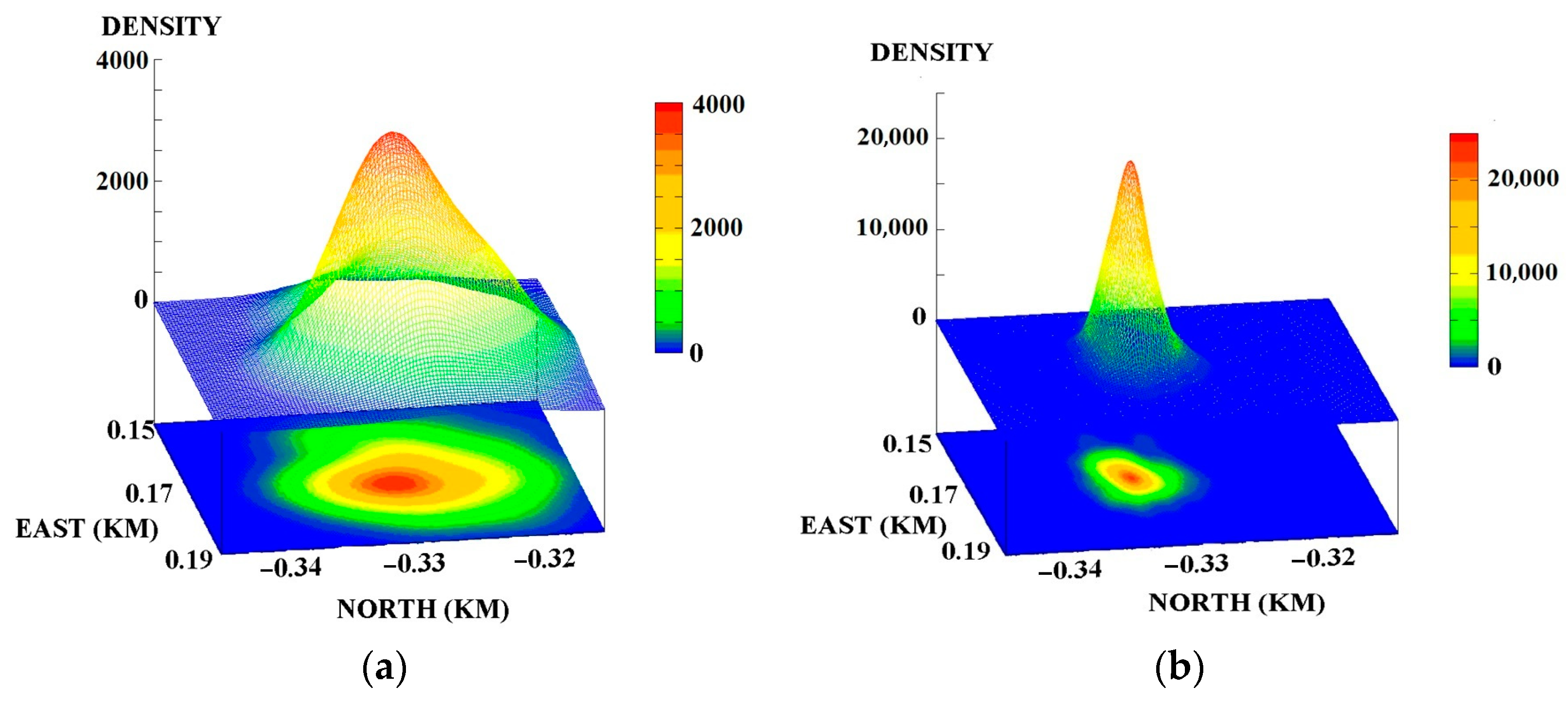
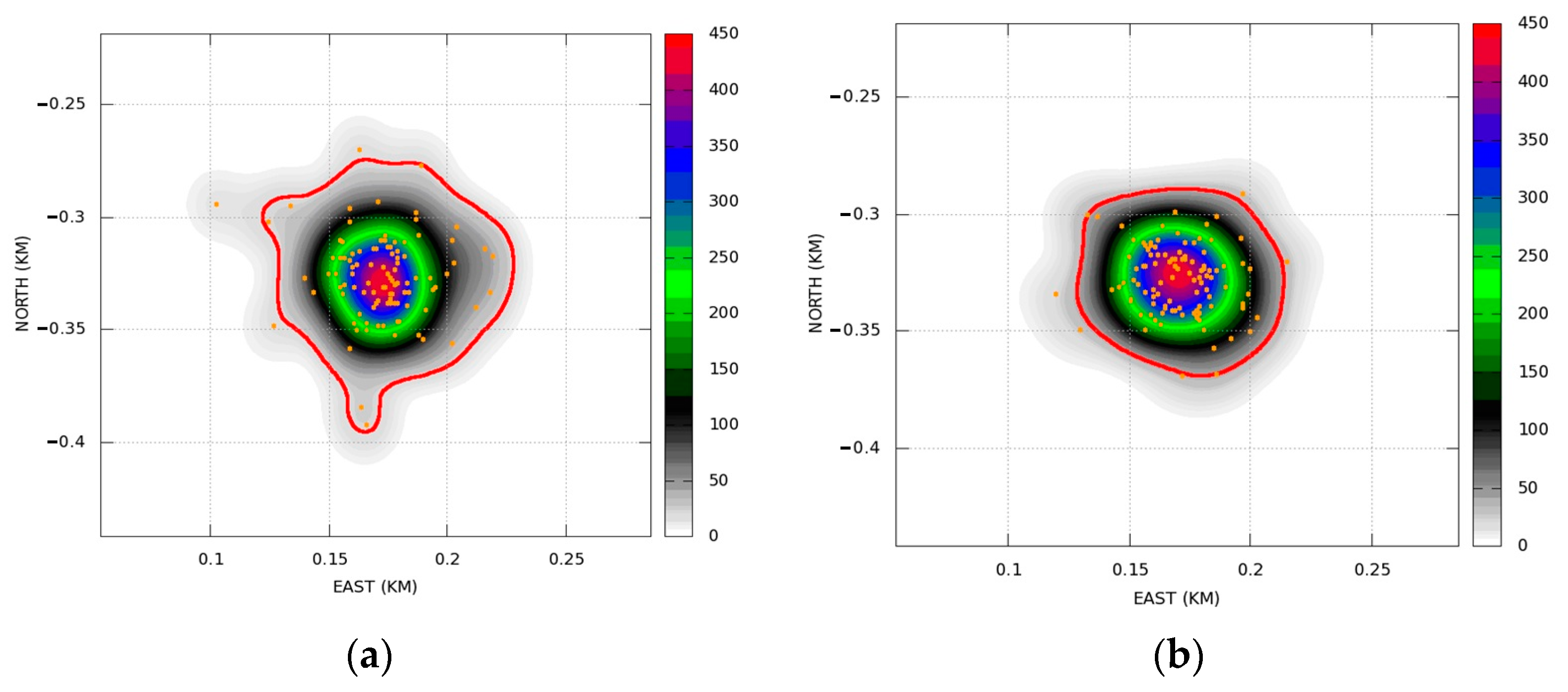
Below, in Figure 1, the empirical two-dimensional probability density functions for averaged (among MLS outputs) signal-to-noise ratio SNR = 0.05 are obtained for 110 independent estimates of source coordinates $\mathbf{v}=\left(v_1,v_2\right)$ in the presence of real correlated noise with matrix power spectral density ${\dot{F}}_{\xi }\left(\lambda \right)$. In Figure 2, similar probability density functions are provided for ${\dot{F}}_{\xi }\left(\lambda \right)=const*\mathbf{I}$, where $\mathbf{I}$ is the unit matrix. That means that ${\xi }_t$ is represented as multidimensional white Gaussian noise with equal power spectral densities.

As can be seen from Figure 1 and Figure 2, in both cases, the ${\rho }_{RMSE}$ value of ${\widehat{u}}_n^{\delta }\left({\dot{\overline{x}}}_{u,n}\right)$ is approximately two times greater than the ${\rho }_{RMSE}$ value of SRP-PHAT. That is, the changing properties of additive noise ${\xi }_t$ lead estimate ${\widehat{u}}_n^{\delta }\left({\dot{\overline{x}}}_{u,n}\right)$ to be more efficient than SRP-PHAT. But while varying the additive noise properties, both estimators show nondramatic changes in estimation accuracy, so they are both robust. More detailed information and a straight numerical comparison are given in [4].

5. Asymptotic Properties of the Objective Function ${\mathit{Q}}_{\mathit{n}}\left({\dot{\overline{x}}}_{u,\mathit{n}};v\right)$

The proof that the objective function $Q_n\left({\dot{\overline{x}}}_{u,n}; v\right)$ satisfies conditions A and C of Theorem 1 consists of a sequence of lemmas.

Lemma 1.

The objective function, $Q_n\left({\dot{\overline{x}}}_{u,n}; v\right)$,$v\in U$, satisfies conditions A  of Theorem 1.

Proof. 

Let us write the Tailor expansion of the objective function $Q_n\left({\dot{\overline{x}}}_{u,n}; u+n^{-1/2}w\right)$ in the vicinity $n^{-1/2}w$, $\left|w\right|<C$ of the parameter value $u$ with the remainder term in the Lagrange form:

$$\begin{gathered} {\displaystyle \sum _{j=1}^n} {\dot{\rho }}_{u,j}^{*}{\dot{\Pi }}_j\left(u+n^{-1/2}w\right){\dot{\rho }}_{u,j}={\displaystyle \sum _{j=1}^n} {\dot{\rho }}_{u,j}^{*}{\dot{\Pi }}_j\left(u\right){\dot{\rho }}_{u,j}+n^{-1/2}{\displaystyle \sum _{j=1}^n} {\dot{\rho }}_{u,j}^{*}\left({\displaystyle \sum _{k=1}^q{\dot{\Pi }}_{k,j}^{\prime }\left(u\right)w_k}\right){\dot{\rho }}_{u,j}- \\ -{\left(2n\right)}^{-1}{\displaystyle \sum _{j=1}^n} {\dot{\rho }}_{u,j}^{*}\left({\displaystyle \sum _{k,l=1}^q{\dot{\Pi }}_{k,l,j}^{″}\left(u\right)w_k{w}_l}\right){\dot{\rho }}_{u,j}+{\beta }_n\left({\dot{\overline{\rho }}}_{u,n}; u,w\right),{\dot{\overline{\rho }}}_{u,n}=\left({\dot{\rho }}_{u,j} j=\overline{1,n}\right),\left|w\right|<C \end{gathered}$$

(19)

where $n^{-1/2}{\dot{\Pi }}_{k,j}^{\prime }\left(u\right)=\frac{\partial }{\partial w_k}{\dot{\Pi }}_j{\left(u+n^{-1/2}w\right)}_{w=0}$; $n^{-1}{\dot{\Pi }}_{k,l,j}^{″}\left(u\right)=\frac{{\partial }^2}{\partial w_k\partial w_l}{\dot{\Pi }}_j{\left(u+n^{-1/2}w\right)}_{\left|w=0\right.}$;

$${\dot{\rho }}_{u,j}={\dot{d}}_j\left(u\right){\dot{s}}_j+{\dot{\eta }}_j.$$

The remainder term ${\beta }_n\left({\dot{\overline{\rho }}}_{u,n}; w\right)$ on the right side of Equation (19) has the form:

$${\beta }_n\left({\dot{\overline{x}}}_{u,n}; w\right)=n^{-3/2}{\displaystyle \sum _{k,l,r}^q{w}_k{w}_l{w}_r\left({\displaystyle \sum _{j=1}^n} {\dot{\rho }}_{u,j}^{*}{\dot{\Pi }}_{k,l,r,j}^{‴}\left(u+n^{-1/2}{\theta }_{k,l,r,j}w\right){\dot{\rho }}_{u,j}\right)},$$

(20)

where $\left|w\right|<C$, ${\theta }_{k,l,r,j}\in \left(0,1\right)$.

We use the Lagrange form of the remainder term ${\beta }_n\left({\dot{\overline{x}}}_{u,n}; w\right)$ above because it is the simplest form of the Tailor expansion of the objective function $Q_n\left({\dot{\overline{x}}}_{u,n};v\right)$ by Equation (13) given on the closed set $v=U$, but this form requires the existence of third bounded partial derivatives of the objective function $Q_n\left({\dot{\overline{x}}}_{u,n};v\right)$. Let us assume that this is true for the sake of simplicity. Due to this assumption, there exists a matrix function:

$${\dot{\Pi }}_{k,l,r,j}^{‴}\left(v\right)={\dot{F}}^{1/2}\left({\lambda }_j\right){\Lambda }_{k,l,r,j}^{‴}\left(v\right){\dot{F}}^{1/2}\left({\lambda }_j\right),$$

(21)

where ${\dot{\Lambda }}_j\left(v\right)=\dot{\Lambda }\left({\lambda }_j;v\right)$; ${\lambda }_j=2\pi j{n}^{-1}$; $\dot{\Lambda }\left(\lambda ;v\right)=\frac{{\dot{F}}_{\xi }^{-1}\left(\lambda \right)\dot{h}\left(\lambda ;v\right){\dot{h}}^{\ast }\left(\lambda ;v\right){\dot{F}}_{\xi }^{-1}\left(\lambda \right)}{{\dot{h}}_j^{*}\left(\lambda ;v\right){\dot{F}}_{\xi }^{-1}\left(\lambda \right)\dot{h}\left(\lambda ;v\right)}$, $v\in U$, which is continuous on $v\in U$ and is bounded for all valid values of its arguments.

In accordance with Equation (7), we have:

$${\dot{\rho }}_{u,j}={\dot{F}}_{\xi ,j}^{-1/2}{\dot{x}}_{u,j}={\dot{d}}_j\left(u\right){\dot{s}}_j+{\dot{\eta }}_j, \mathrm{where} {\dot{d}}_j\left(v\right)={\dot{F}}_{\xi ,j}^{-1/2}{\dot{h}}_j\left(v\right).$$

The term ${\dot{d}}_j\left(u\right){\dot{s}}_j$ is bounded for all $j\in \overline{1,n}$, $u\in \tilde{U}\subset U$. The pairs of random vectors ${\dot{\eta }}_j, {\dot{\eta }}_k$, $j\ne k\in \overline{1,n}$ are mutually asymptotically independent for $n\to \infty$; the Gaussian random vectors ${\dot{\eta }}_j$ have asymptotic covariance matrices equal to $I$ for $n\to \infty$. That is, we have (see Appendix A):

$$\mathrm{E}\left\{{\dot{\eta }}_j\right\}=0, j\in \overline{1,n}; \mathrm{E}\left\{{\dot{\eta }}_j{\dot{\eta }}_k^{\ast }\right\}={\dot{F}}_j^{-1/2}\mathrm{E}\left\{{\dot{\xi }}_j{\dot{\xi }}_k^{\ast }\right\}{\dot{F}}_k^{-1/2}=‖{\dot{O}}_{j,k}^{\eta }‖, j\ne k\in \overline{1,n};$$

$$\mathrm{E}\left\{{\dot{\eta }}_j{\dot{\eta }}_j^{\ast }\right\}={\dot{F}}_j^{-1/2}\mathrm{E}\left\{{\dot{\xi }}_j{\dot{\xi }}_j^{\ast }\right\}{\dot{F}}_j^{-1/2}={\dot{F}}_j^{-1/2}\left[{\dot{F}}_j+{\dot{O}}_j^{\xi }\right]{\dot{F}}_j^{-1/2}=I+{\dot{O}}_j^{\eta },$$

(22)

where $‖{\dot{O}}_j^{\eta }‖\le C{n}^{-1-\beta }$, $\beta \in \left(0,1\right)$ for all $j\in \overline{1,n}$.

Taking into account Equation (21) and the boundedness of the terms $w_k{w}_l{w}_r$ in Equation (20), we conclude that the sequence of random variables ${\beta }_n\left({\dot{\overline{\rho }}}_{u,n}; w\right)$ tends to zero in probability as $n\to \infty$, in accordance with the Law of Large Numbers [18] (Lemma 2.4):

$$P-\underset{n\to \infty }{\lim } n^{-3/2}{\displaystyle \sum _{j=1}^n} {\displaystyle \sum _{k,l,r}^q w_k{w}_l{w}_r{\dot{\rho }}_{{\dot{x}}_{u,j}}^{*}{\dot{\Pi }}_{k,l,r,j}^{‴}\left(u+n^{-1/2}{\theta }_{k,l,r,j}w\right){\dot{\rho }}_{{\dot{x}}_{u,j}}}=0.$$

(23)

□

Let us assume that the vector statistic

$$n^{-1/2}{\delta }_n\left({\dot{\overline{x}}}_{u,n}; u\right)=\left(n^{-1/2}{\delta }_{k,n}\left({\dot{\overline{x}}}_{u,n}; u\right), k\in \overline{1,q}\right),$$

where $n^{-1/2}{\delta }_{k,n}\left({\dot{\overline{x}}}_{u,n}; u\right)=\left(n^{-1/2}{\displaystyle \sum _{j=1}^n} {\dot{\rho }}_{u,j}^{*}{\dot{\Pi }}_{k,j}^{\prime }{\left(v\right)}_{\left|v=u\right.}{\dot{\rho }}_{u,j}, k=\overline{1,q}\right)=$

$$=n^{-1/2}{\displaystyle \sum _{j=1}^n{\left({\dot{d}}_j\left(u\right){\dot{s}}_j+{\dot{\eta }}_j\right)}^{\ast }{\dot{\Pi }}_{k,j}^{\prime }\left(u\right)\left({\dot{d}}_j\left(u\right){\dot{s}}_j+{\dot{\eta }}_j\right)},$$

(24)

particularly satisfies conditions B of Theorem 1. That is, $n^{-1/2}{\delta }_n\left({\dot{\overline{x}}}_{u,n}; u\right)$ has a Gaussian limit distribution. Let us prove that the moments of this distribution are

$$\underset{n\to \infty }{\lim } \mathrm{E}\left\{n^{-1/2}{\delta }_n\left({\dot{\overline{x}}}_{u,n};u\right)\right\}=0; \underset{n\to \infty }{\lim } \mathrm{E}\left\{n^{-1}{\delta }_n\left({\dot{\overline{x}}}_{u,n};u\right){\delta }_n^{\mathrm{T}}\left({\dot{\overline{x}}}_{u,n};u\right)\right\}=\Psi \left(u\right); ‖\Psi \left(u\right)‖<C.$$

Lemma 2.

The statistics given by (24):

$$\begin{gathered} n^{-1/2}{\delta }_{k,n}\left({\dot{\overline{x}}}_{u,n};u\right)=n^{-1/2}{\displaystyle \sum _{j=1}^n{\dot{d}}_j^{*}\left(u\right){\dot{\Pi }}_{k,j}^{\prime }\left(u\right){\dot{d}}_j\left(u\right){\left|s_j\right|}^2}+n^{-1/2}{\displaystyle \sum _{j=1}^n{\dot{\eta }}_j^{\ast }{\dot{\Pi }}_{k,j}^{\prime }\left(u\right){\dot{\eta }}_j}+ \\ +2n^{-1/2}{\displaystyle \sum _{j=1}^n\mathrm{Re}\left({\dot{\eta }}_j^{\ast }{\dot{\Pi }}_{k,j}^{\prime }\left(u\right){\dot{d}}_j\left(u\right){\dot{s}}_j\right)}, k=\overline{1,q} \end{gathered}$$

(25)

have zero mean in the asymptotic $n\to \infty$:

$$\underset{n\to \infty }{\lim } \mathrm{E}\left\{n^{-1/2}{\delta }_k\left({\dot{\overline{x}}}_{u,n}; u\right)\right\}=0, k\in \overline{1,q}.$$

Proof of Lemma 2.

The term ${\dot{\Pi }}_{k,j}^{\prime }\left(u\right)$ has the following form:

$$\begin{gathered} {\dot{\Pi }}_{k,j}^{\prime }\left(u\right)=-\frac{\partial }{\partial v_k}\left[\frac{{\dot{d}}_v{\dot{d}}_v^{\ast }}{{\left|d_v\right|}^2}\right]=-{\left|d_v\right|}^{-4}{\left[\frac{\partial \left[{\dot{d}}_v{\dot{d}}_v^{\ast }\right]}{\partial v_k}\left(d_v^{\ast }{d}_v\right)-\left[{\dot{d}}_v{\dot{d}}_v^{\ast }\right]\frac{\partial \left(d_v^{\ast }{d}_v\right)}{\partial v_k}\right]}_{\left|v=u\right.}= \\ =-{\left|d_u\right|}^{-4}\left[\left[{{\dot{d}}^{\prime }}_{k,u}{\dot{d}}_u^{\ast }\right]{\left|{\dot{d}}_u\right|}^2+\left[d_u{d^{\prime }}_{k,u}^{\ast }\right]{\left|{\dot{d}}_u\right|}^2-\left[{\dot{d}}_u{\dot{d}}_u^{\ast }\right]\left({d^{\prime }}_{k,u}^{\ast }{d}_u\right)-\left[{\dot{d}}_u{\dot{d}}_u^{\ast }\right]\left(d_u^{\ast }{d}_{k,u}^{\prime }\right)\right], \end{gathered}$$

(26)

where $u\in \tilde{U}, j\in \overline{1,n}, k\in \overline{1,q}.$

Statement 1.

The first term on the right side of Equation (25) is equal to zero:

$$n^{-1/2}{\displaystyle \sum _{j=1}^n{\dot{d}}_j^{*}\left(u\right){\dot{\Pi }}_{k,j}^{\prime }\left(v\right){\dot{d}}_j\left(u\right){\left|s_j\right|}^2}=0 \mathrm{for} \mathrm{all} k\in \overline{1,q}.$$

Proof of Statement 1.

Let us rewrite the terms ${\dot{d}}_j^{*}\left(u\right){\dot{\Pi }}_{k,j}^{\prime }\left(u\right){\dot{d}}_j\left(u\right)$ for any $j\in \overline{1,n}, n>q$, $k\in \overline{1,q}$ using the associative law for products of several vectors:

$$\begin{gathered} {\dot{d}}_j^{*}\left(u\right){\dot{\Pi }}_{k,j}^{\prime }\left(u\right){\dot{d}}_j\left(u\right)=-{\left|d_u\right|}^{-4}\left[{\left|{\dot{d}}_u\right|}^2{\dot{d}}_u^{\ast }\left[{\dot{d}}_{k,u}^{\prime }{\dot{d}}_u^{\ast }\right]{\dot{d}}_u+{\dot{d}}_u^{\ast }\left[d_u{\dot{d}}_{k,u}^{\prime \ast }\right]{\dot{d}}_u{\left|{\dot{d}}_u\right|}^2\right]+ \\ +{\left|d_u\right|}^{-4}\left[{\dot{d}}_u^{\ast }\left[{\dot{d}}_u{\dot{d}}_u^{\ast }\right]{\dot{d}}_u\left(d_u^{\ast }{\dot{d}}_{k,u}^{\prime }\right)+{\dot{d}}_u^{\ast }\left[{\dot{d}}_u{\dot{d}}_u^{\ast }\right]{\dot{d}}_u\left(d_u^{\ast }{\dot{d}}_{k,u}^{\prime }\right)\right]= \\ =-{\left|d_u\right|}^{-4}\left({\left|d_u\right|}^2\left(d_u^{\ast }{\dot{d}}_{k,u}^{\prime }\right){\left|d_u\right|}^2+{\left|d_u\right|}^2\left({\dot{d}}_{k,u}^{\prime \ast }{d}_u\right){\left|d_u\right|}^2\right)+ \\ +{\left|d_u\right|}^{-4}\left({\left|d_u\right|}^2{\left|d_u\right|}^2\left(d_u^{\ast }{d^{\prime }}_{k,u}\right)+{\left|d_u\right|}^2{\left|d_u\right|}^2\left(d_u^{\ast }{\dot{d}}_{k,u}^{\prime }\right)\right)\equiv 0 \mathrm{for} \mathrm{any} j\in \overline{1,n}, n>q, k\in \overline{1,q}. \end{gathered}$$

□

The mathematical expectation of the last term on the right side of Equation (25) is also equal to zero due to Equation (22): $2n^{-1/2}{\displaystyle \sum _{j=1}^n\mathrm{Re}\left(\mathrm{E}\left\{{\dot{\eta }}_j^{\ast }\right\}{\dot{\Pi }}_{k,j}^{\prime }\left(u\right){\dot{d}}_j\left(u\right){\dot{s}}_j\right)}=0$.

Statement 2.

The limit of the mathematical expectation of the second term on the right side of Equation (25) is equal to zero:

$$n^{-1/2}\underset{n\to \infty }{\lim } {\displaystyle \sum _{j=1}^n\mathrm{E}\left\{{\dot{\eta }}_j^{\ast }{\dot{\Pi }}_{k,j}^{\prime }\left(u\right){\dot{\eta }}_j\right\}=}{n}^{-1/2}\underset{n\to \infty }{\lim } {\displaystyle \sum _{j=1}^{n}tr\left[{\dot{\Pi }}_{k,j}^{\prime }\left(u\right)\mathrm{E}\left\{{\dot{\eta }}_j{\dot{\eta }}_j^{\ast }\right\}\right]}=0.$$

Proof of Statement 2.

As follows from Equation (22):

$$tr\left[{\dot{\Pi }}_{k,j}^{\prime }\left(u\right)\mathrm{E}\left\{{\dot{\eta }}_j{\dot{\eta }}_j^{\ast }\right\}\right]=tr{\dot{\Pi }}_{k,j}^{\prime }\left(u\right)+tr\left[{\dot{\Pi }}_{k,j}^{\prime }\left(u\right){\dot{O}}_j^{\eta }\right],$$

(27)

where $‖{\dot{O}}_j^{\eta }‖\le C{n}^{-1-\beta }$, $\beta \in \left(0,1\right)$ for all $j\in \overline{1,n}$.

Let us first prove that $tr{\dot{\Pi }}_{k,j}^{\prime }\left(u\right)=0$ for any $u\in \tilde{U}, k\in \overline{1,q}; j\in \overline{1,n}, n>q$. The following equalities are held:

$$\begin{gathered} \mathrm{tr}{\dot{\Pi }}_j\left(u\right)=tr\left[I-{\dot{d}}_j\left(u\right){\left|{\dot{d}}_j\left(u\right)\right|}^{-2}{\dot{d}}_j^{*}\left(u\right)\right]=m-{\left|{\dot{d}}_j\left(u\right)\right|}^{-2}\mathrm{tr}\left[d_j\left(u\right)d_j^{*}\left(u\right)\right]= \\ =m-{\left|{\dot{d}}_j\left(u\right)\right|}^{-2}{\displaystyle \sum _{l=1}^m{\dot{d}}_{l,j}\left(u\right){\dot{d}}_{l,j}^{*}\left(u\right)}=m-{\left|{\dot{d}}_j\left(u\right)\right|}^{-2}{\left|{\dot{d}}_j\left(u\right)\right|}^2=m-1. \end{gathered}$$

Therefore, $tr{\dot{\Pi }}_{k,j}^{\prime }\left(u\right)=\frac{\partial }{\partial v_k}tr{\dot{\Pi }}_j{\left(v\right)}_{\left|v=u\right.}\equiv 0$ for any $u\in \tilde{U}, k\in \overline{1,q}; j\in \overline{1,n}, n>q$. Consequently:

$$n^{-1/2}{\displaystyle \sum _{j=1}^{n}tr\left[{\dot{\Pi }}_{k,j}^{\prime }\left(u\right)\mathrm{E}\left\{{\dot{\eta }}_j{\dot{\eta }}_j^{\ast }\right\}\right]}=n^{-1/2}{\displaystyle \sum _{j=1}^n\frac{\partial }{\partial v_k}\mathrm{tr}\left[{\dot{\Pi }}_j{\left(v\right)}_{\left|v=u\right.}{\dot{O}}_j^{\eta }\right]},$$

(28)

where $‖{\dot{O}}_j^{\eta }‖\le C{n}^{-1-\beta }$, $\beta \in \left(0,1\right)$.

The matrix functions ${\dot{\Pi }}_j\left(v\right)$ have continuous partial derivatives with respect to $v_k$ for any $v\in U$, $j\in \overline{1,n}$. Consequently, $‖{{\dot{\Pi }}^{\prime }}_{k,j}\left(v\right)‖\le C_1$ for any $v\in U$,$j\in \overline{1,n}$. As follows from Equation (28):

$$\underset{n\to \infty }{\lim } n^{-1/2}\left|\underset{v\in U}{sup}{\displaystyle \sum _{j=1}^n\mathrm{tr}\left[{\dot{\Pi }}_{k,j}^{\prime }\left(v\right){\dot{O}}_j^{\eta }\left(n^{-1-\beta }\right)\right]}\right|\le C{n}^{-1/2-\beta }=0.$$

(29)

Finally, we deduce from (26)–(29) that

$$\underset{n\to \infty }{\lim } n^{-1/2}{\displaystyle \sum _{j=1}^n\mathrm{E}\left\{{\dot{\eta }}_j{ }^{\ast }{\dot{\Pi }}_{k,j}^{\prime }\left(v\right){\dot{\eta }}_j\right\}}=0.$$

(30)

□ □

It follows from Lemmas 1 and 2 that the components of the family of statistics $n^{-1/2}\delta \left({\dot{\overline{x}}}_{u,n};v\right), v\in U$ in the limit $n\to \infty$ have a zero mathematical expectation:

$$\underset{n\to \infty }{\lim } E\left\{n^{-1/2}{\delta }_k\left({\dot{\overline{x}}}_{u,n};u\right)\right\}=\underset{n\to \infty }{\lim } E\left(n^{-1/2}{\displaystyle \sum _{j=1}^n{\dot{\eta }}_{u,j}^{\ast }{\dot{\Pi }}_{k,j}^{\prime }\left(u\right){\dot{\eta }}_{u,j}}+2n^{-1/2}{\displaystyle \sum _{j=1}^n\mathrm{Re}\left({\dot{\eta }}_{u,j}^{\ast }{\dot{\Pi }}_{k,j}^{\prime }\left(u\right){\dot{d}}_j\left(u\right){\dot{s}}_j\right)}\right)=0.$$

Lemma 3.

The covariance matrix $\Psi \left(u\right)$ of the statistic $n^{-1/2}\delta \left({\dot{\overline{x}}}_{u,n};u\right)$ has the limit

$$\underset{n\to \infty }{lim}\mathrm{E}\left\{n^{-1}\delta \left({\dot{\overline{x}}}_{u,n};u\right){\delta }^T\left({\dot{\overline{x}}}_{u,n};u\right)\right\}=\Psi \left(u\right)=\left[{\Psi }_{k,l}\left(u\right), k,l\in \overline{1,q}\right], ‖\Psi \left(u\right)‖<C<\infty ,$$

where ${\Psi }_{k,l}\left(u\right)=2{\displaystyle \underset{-\pi }{\overset{\pi }{\int }}\mathrm{tr}\left[\left({\dot{\Lambda }}_k^{\prime }\left(\lambda ;u\right){\dot{F}}_{\xi }\left(\lambda \right){\dot{\Lambda }}_l^{\prime }\left(\lambda ;u\right){\dot{F}}_{\xi }\left(\lambda \right)\right)d\lambda \right]}$ + $4{\displaystyle \underset{-\pi }{\overset{\pi }{\int }}{\dot{h}}^{*}\left(\lambda ;u\right){\dot{\Lambda }}_k^{\prime }\left(\lambda ;u\right){\dot{F}}_{\xi }\left(\lambda \right){\dot{\Lambda }}_l^{\prime }\left(\lambda ;u\right)} \dot{h}\left(\lambda ;u\right)d{w}_{\mathrm{s}}\left(\lambda \right)$; $k,l\in \overline{0,q}$, $w_{\mathrm{s}}\left(\lambda \right)=\underset{n\to \infty }{\lim } n^{-1}{\displaystyle \sum _{j=1}^{{\nu }_{\lambda }}{\left|\dot{s}\left(2\pi j{n}^{-1}\right)\right|}^2}$; ${\nu }_{\lambda }=\left[\lambda \right]$ is the largest integer n for which $2\pi j{n}^{-1}\le \lambda$; $\dot{\Lambda }\left(\lambda ;v\right)=\frac{{\dot{F}}_{\xi }^{-1}\left(\lambda \right)\dot{h}\left(\lambda ;v\right){\dot{h}}^{\ast }\left(\lambda ;v\right){\dot{F}}_{\xi }^{-1}\left(\lambda \right)}{{\dot{h}}_j^{*}\left(\lambda ;v\right){\dot{F}}_{\xi }^{-1}\left(\lambda \right)\dot{h}\left(\lambda ;v\right)}$; ${\dot{\Lambda }}_k^{\prime }\left(\lambda ;u\right)=\frac{\partial }{\partial v_k}\Lambda {\left(\lambda ;v\right)}_{\left|v=u\right.}$.

Proof of Lemma 3.

According to Lemma 2, $\underset{n\to \infty }{\lim } \mathrm{E}\left\{n^{-1/}{\delta }_k\left({\dot{\overline{x}}}_{u,n};u\right)\right\}=0$, $k\in \overline{1,q}$. Consequently,

$${\mathrm{\Psi }}_{k,l}\left(u\right)=\underset{n\to \infty }{\lim } \mathrm{E}\left\{n^{-1}{\delta }_{n,k}\left({\dot{\overline{x}}}_{u,n};u\right) {\delta }_{n,l}\left({\dot{\overline{x}}}_{u,n};u\right)\right\}.$$

According to Equation (25) and Statement S.1, we have:

$$n^{-1/2}\delta \left({\dot{\overline{x}}}_{u,n};u\right)=n^{-1/2}{\displaystyle \sum _{j=1}^n\left({\dot{\eta }}_j{ }^{\ast }{\dot{\Pi }}_{k,j}^{\prime }\left(u\right){\dot{\eta }}_j+2\mathrm{Re}{\dot{\eta }}_j^{\ast }{\dot{\Pi }}_{k,j}^{\prime }\left(u\right){\dot{d}}_j\left(u\right){\dot{s}}_j\right)}.$$

(31)

Therefore, ${\mathrm{\Psi }}_{k,l}\left(u\right)$ can be written as:

$${\mathrm{\Psi }}_{k,l}\left(u\right)=\underset{n\to \infty }{\lim } n^{-1}{\displaystyle \sum _{i=1}^n{\displaystyle \sum _{j=1}^n\mathrm{E}\left\{Q_{k,i}{Q}_{l,j}+Q_{k,i}{L}_{l,j}+L_{k,i}{Q}_{l,j}+L_{k,i}{L}_{l,j}\right\}}},$$

(32)

where $Q_{k,j}={\dot{\eta }}_j{ }^{\ast }{\dot{\Pi }}_{k,j}^{\prime }\left(u\right){\dot{\eta }}_j$; $L_{k,j}=2\mathrm{Re}\left({\dot{\eta }}_i^{\ast }{\dot{\Pi }}_{k,j}^{\prime }\left(u\right){\dot{d}}_j\left(u\right){\dot{s}}_j\right)$.

The double sum on the right side of Equation (32) can be calculated as:

$$\begin{gathered} {\mathrm{\Psi }}_{k,l}\left(u\right)=\underset{n\to \infty }{lim}{n}^{-1}{\displaystyle \sum _{j=1}^n\mathrm{E}\left\{Q_{k,j}{Q}_{l,j}+Q_{k,j}{L}_{l,j}+L_{k,j}{Q}_{l,j}+L_{k,j}{L}_{l,j}\right\}}+ \\ +\underset{n\to \infty }{\lim } n^{-1}{\displaystyle \sum _{i=1}^n{\displaystyle \sum _{\left|j-i\right|=1}^n\mathrm{E}\left\{Q_{k,i}{Q}_{l,j}+Q_{k,i}{L}_{l,j}+L_{k,i}{Q}_{l,j}+L_{k,i}{L}_{l,j}\right\}}}=A_{k,l}+B_{k,l}. \end{gathered}$$

(33)

According to (23), the complex vectors ${\dot{\eta }}_j, j\in \overline{1,n}$ become mutually independent for large values of n:

$\mathrm{E}\left\{{\dot{\eta }}_i{\dot{\eta }}_j^{\ast }\right\}={\dot{O}}_{i,j}^{\eta }\left(n^{-1-\beta }\right)$, where $‖{\dot{O}}_{i,j}^{\eta }\left(n^{-1-\beta }\right)‖\le \overline{C}{n}^{-1-\beta }$, $\beta \in \left(0,1\right)$. It is easy to show that the term $B_{k,l}$ in Equation (33) has the form:

$$\begin{gathered} B_{k,l}=\underset{n\to \infty }{\lim } n^{-1}{\displaystyle \sum _{i=1}^n\mathrm{E}\left(Q_{k,i}\right){\displaystyle \sum _{\left|j-i\right|=1}^n\mathrm{E}\left(Q_{l,j}\right)+}} \\ +\underset{n\to \infty }{\lim } n^{-1}{\displaystyle \sum _{i=1}^n{\displaystyle \sum _{\left|j-i\right|=1}^n\left(\mathrm{E}\left\{Q_{k,i}\right\}\mathrm{E}\left\{L_{l,j}\right\}+\mathrm{E}\left\{L_{k,i}\right\}\mathrm{E}\left\{Q_{l,j}\right\}+\mathrm{E}\left\{L_{k,i}\right\}\mathrm{E}\left\{L_{l,j}\right\}\right)}}. \end{gathered}$$

(34)

The first limit on the right side of (34) is equal to zero due to Statement S1:

$$\underset{n\to \infty }{\lim } n^{-1}{\displaystyle \sum _{i=1}^n\mathrm{E}\left(Q_{k,i}\right){\displaystyle \sum _{j\ne i\in \overline{1,n}}\mathrm{E}\left(Q_{l,j}\right)}}\le \underset{n\to \infty }{lim}{n}^{-1/2}{\displaystyle \sum _{i=1}^n\mathrm{E}\left\{Q_{k,i}\right\}\underset{n\to \infty }{lim}{n}^{-1/2}{\displaystyle \sum _{j=1}^n\mathrm{E}\left\{Q_{l,j}\right\}}}=0.$$

The second limit on the right side of (34) is also equal to zero since $\mathrm{E}\left\{{\dot{\eta }}_j\right\}=0$. Hence,

$$\mathrm{E}\left\{L_{k,j}\right\}=2\mathrm{Re}\mathrm{E}\left\{{\dot{\eta }}_j^{\ast }\right\}{\dot{\Pi }}_{k,j}^{\prime }\left(u\right){\dot{d}}_j\left(u\right){\dot{s}}_j=0, k\in \overline{1,q}, j\in \mathbb{N}.$$

As a result, we obtain:

$${\mathrm{\Psi }}_{k,l}\left(u\right)=\underset{n\to \infty }{lim}{n}^{-1}{\displaystyle \sum _{j=1}^n\left(\mathrm{E}\left\{Q_{k,j}{L}_{l,j}\right\}+\mathrm{E}\left\{Q_{l,j}{L}_{k,j}\right\}\right)}+\underset{n\to \infty }{lim}{n}^{-1}{\displaystyle \sum _{j=1}^n\left(\mathrm{E}\left\{Q_{k,j}{Q}_{l,j}\right\}+\mathrm{E}\left\{L_{k,j}{L}_{l,j}\right\}\right)}.$$

(35)

The quantities $\mathrm{E}\left\{Q_{k,j}{L}_{l,j}\right\}=\mathrm{E}\left\{{\dot{\eta }}_j{ }^{\ast }{\dot{\Pi }}_{k,j}^{\prime }\left(u\right){\dot{\eta }}_j\times 2\mathrm{Re}\left({\dot{\eta }}_j^{\ast }{\dot{\Pi }}_{l,j}^{\prime }\left(u\right){\dot{d}}_j\left(u\right){\dot{s}}_j\right)\right\}$, $k,l\in \overline{1,q}$ are the sums of terms having the forms $\mathrm{E}\left\{{\eta }_{s,j}{\eta }_{r,j}{\eta }_{w,j}\right\}{a}_{s,r,j}{b}_{w,j}$. That is, they are the sums of the products of three random variables having Gaussian distributions with zero mean values. The factors in these products belong to the sets $\left\{{\eta }_{k,j}^{\mathrm{re}}, k\in \overline{1,q}\right\}$, $\left\{{\eta }_{k,j}^{\mathrm{im}}, k\in \overline{1,q}\right\}$. Due to the properties of Gaussian distributions, the mathematical expectations of these products are equal to zero.

Consequently,

$$\underset{n\to \infty }{lim}{n}^{-1}{\displaystyle \sum _{j=1}^n\mathrm{E}\left\{Q_{k,j}{L}_{l,j}\right\}}=0, j\in \overline{1,n}, k,l\in \overline{1,q}.$$

Thus, we finally obtain

$$\begin{gathered} {\mathrm{\Psi }}_{k,l}\left(u\right)=\underset{n\to \infty }{lim}{n}^{-1}{\displaystyle \sum _{j=1}^n\left(\mathrm{E}\left\{Q_{k,j}{Q}_{l,j}\right\}+\mathrm{E}\left\{L_{k,j}{L}_{l,j}\right\}\right)}= \\ =\underset{n\to \infty }{\lim } n^{-1}{\displaystyle \sum _{j=1}^n\mathrm{E}\left\{\left({\dot{\eta }}_j{ }^{\ast }{\dot{\Pi }}_{k,j}^{\prime }\left(u\right){\dot{\eta }}_j\right)\left({\dot{\eta }}_j{ }^{\ast }{\dot{\Pi }}_{l,j}^{\prime }\left(u\right){\dot{\eta }}_j\right)\right\}}+ \\ +4\underset{n\to \infty }{\lim } n^{-1}{\displaystyle \sum _{j=1}^n\mathrm{E}\left\{\mathrm{Re}\left({\dot{\eta }}_j^{\ast }{\dot{\Pi }}_{k,j}^{\prime }\left(u\right){\dot{d}}_j\left(u\right){\dot{s}}_j\right)\mathrm{Re}\left({\dot{\eta }}_j^{\ast }{\dot{\Pi }}_{l,j}^{\prime }\left(u\right){\dot{d}}_j\left(u\right){\dot{s}}_j\right)\right\}}. \end{gathered}$$

(36)

To find the expression for the mathematical expectation $E\left\{\left({\dot{\eta }}_j{ }^{\ast }{\dot{\Pi }}_{k,j}^{\prime }\left(u\right){\dot{\eta }}_j\right)\left({\dot{\eta }}_j{ }^{\ast }{\dot{\Pi }}_{l,j}^{\prime }\left(u\right){\dot{\eta }}_j\right)\right\}$, we can use the following theorem proven in [20] (Theorem 5.2c, p. 109):

Theorem 2.

If the random vector $\dot{y}$ has the complex Gaussian distribution ${\mathfrak{N}}_C\left(0,\dot{{\rm K}}\right)$, then the covariance of the product of quadratic forms $\left({\dot{y}}^{\mathrm{T}}\dot{A}\dot{y}\right)\left({\dot{y}}^{\mathrm{T}}\dot{B}\dot{y}\right)$, where $\dot{A}$ u $\dot{B}$ are Hermitian matrices, is determined by the following equation: $\mathrm{E}\left\{(y^{\mathrm{T}}\dot{A}y)(y^{\mathrm{T}}\dot{B}y)\right\}=2\mathrm{tr}[\dot{A}\dot{{\rm K}}\dot{B}\dot{{\rm K}}]$.

Using this theorem when $\dot{y}=\dot{\eta }$, ${\mathfrak{N}}_C\left(0,\dot{{\rm K}}\right)=\mathfrak{N}\left(0,I\right)$, $\dot{A}={\dot{\Pi }}_{k,j}^{\prime }$, $\dot{B}={\dot{\Pi }}_{l,j}^{\prime }$, we obtain:

$$\mathrm{E}\left\{\left({\dot{\eta }}_j{ }^{\ast }{\dot{\Pi }}_{k,j}^{\prime }\left(u\right){\dot{\eta }}_j\right)\left({\dot{\eta }}_j{ }^{\ast }{\dot{\Pi }}_{l,j}^{\prime }\left(u\right){\dot{\eta }}_j\right)\right\}=2\mathrm{tr}\left[{\dot{\Pi }}_{k,j}^{\prime }\left(u\right){\dot{\Pi }}_{l,j}^{\prime }\left(u\right)\right].$$

(37)

Since ${\dot{\Pi }}_{k,j}^{\prime }\left(u\right)={\dot{F}}_{ }^{1/2}\left({\lambda }_j\right){{\dot{\Lambda }}^{\prime }}_{k,j}\left({\lambda }_j;u\right){\dot{F}}^{1/2}\left({\lambda }_j\right)$, the first term on the right side of (37) takes the following form:

$$\begin{gathered} \underset{n\to \infty }{\lim } n^{-1}{\displaystyle \sum _{j=1}^n\mathrm{E}\left\{\left({\dot{\eta }}_j{ }^{\ast }{\dot{\Pi }}_{k,j}^{\prime }\left(u\right){\dot{\eta }}_j\right)\left({\dot{\eta }}_j{ }^{\ast }{\dot{\Pi }}_{l,j}^{\prime }\left(u\right){\dot{\eta }}_j\right)\right\}}= \\ =\underset{n\to \infty }{\lim } 2n^{-1}{\displaystyle \sum _{j=1}^n\mathrm{tr}\left[{\dot{F}}^{1/2}\left({\lambda }_j\right){\dot{\Lambda }}_{k,j}^{\prime }\left({\lambda }_j;u\right){\dot{F}}^{1/2}\left({\lambda }_j\right){\dot{F}}^{1/2}\left({\lambda }_j\right){\dot{\Lambda }}_{l,j}^{\prime }\left({\lambda }_j;u\right){\dot{F}}^{1/2}\left({\lambda }_j\right)\right]}= \\ =2{\displaystyle \underset{0}{\overset{2\pi }{\int }}\mathrm{tr}\left[{\dot{\Lambda }}_k^{\prime }\left(\lambda ;u\right)\dot{F}\left(\lambda \right){\dot{{\Lambda }^{\prime }}}_l\left(\lambda ;u\right)\dot{F}\left(\lambda \right)\right]}d\lambda . \end{gathered}$$

(38)

Let us find an expression for the last term on the right side of Equation (36):

$$4\underset{n\to \infty }{\lim } n^{-1}{\displaystyle \sum _{j=1}^n\mathrm{E}\left\{\mathrm{Re}\left({\dot{\eta }}_j^{\ast }{\dot{\Pi }}_{k,j}^{\prime }\left(u\right){\dot{d}}_j\left(u\right){\dot{s}}_j\right)\mathrm{Re}\left({\dot{\eta }}_j^{\ast }{\dot{\Pi }}_{l,j}^{\prime }\left(u\right){\dot{d}}_j\left(u\right){\dot{s}}_j\right)\right\}}.$$

(39)

Since ${\dot{\Pi }}_{k,j}^{\prime }\left(u\right), k\in \overline{1,q}$ are Hermitian matrices, then the terms of sum (39) can be rewritten as $\mathrm{E}\left\{\mathrm{Re}\left({\dot{a}}^{\ast }\dot{C}\dot{b}\right)\mathrm{Re}\left({\dot{a}}^{\ast }B\dot{b}\right)\right\}$, where $\dot{a}={\dot{\eta }}_j$; $\dot{b}={\dot{d}}_j\left(u\right){\dot{s}}_j$; $\dot{C}={\dot{\Pi }}_{k,j}^{\prime }\left(u\right)$; $\dot{B}={\dot{\Pi }}_{l,j}^{\prime }\left(u\right)$. The following equalities are valid for the Hermitian matrices $\dot{C}$, $\dot{B}$ and for the vectors $\dot{a}, \dot{b}$:

$$\begin{gathered} 2\mathrm{Re}\left({\dot{a}}^{\ast }\dot{C}\dot{b}\right)2\mathrm{Re}\left({\dot{a}}^{\ast }B\dot{b}\right)=\left({\dot{a}}^{\ast }\dot{C}\dot{b}+{\left({\dot{a}}^{\ast }\dot{C}\dot{b}\right)}^{\ast }\right)\left({\dot{a}}^{\ast }\dot{B}\dot{b}+{\left({\dot{a}}^{\ast }\dot{B}\dot{b}\right)}^{\ast }\right)=\left({\dot{a}}^{\ast }\dot{C}\dot{b}+{\dot{b}}^{\ast }{\dot{C}}^{\ast }\dot{a}\right)\left({\dot{a}}^{\ast }B\dot{b}+{\dot{b}}^{\ast }{B}^{\ast }\dot{a}\right)= \\ =\left({\dot{a}}^{\ast }p+{\dot{p}}^{\ast }\dot{a}\right)\left({\dot{a}}^{\ast }\dot{q}+{\dot{q}}^{\ast }\dot{a}\right)=\left(2{\dot{a}}^{\ast }p\right)\left(2{\dot{q}}^{\ast }\dot{a}\right)=4\dot{a}\dot{C}\dot{b}{\dot{b}}^{\ast }\dot{B}\dot{a}, \end{gathered}$$

where $\dot{p}=\dot{C}\dot{b}, \dot{q}=\dot{B}\dot{b}$ and ${\dot{a}}^{\ast }p={\dot{p}}^{\ast }\dot{a}$ due to the property of the scalar product, and $\dot{C}={\dot{C}}^{\ast }, \dot{B}={\dot{B}}^{\ast }$ due to the property of Hermitian matrices. Since ${\dot{\eta }}_j={\dot{F}}_{\xi ,j}^{-1/2}{\dot{\xi }}_j; {\dot{d}}_j\left(u\right)={\dot{F}}_{\xi ,j}^{-1/2}{\dot{h}}_j\left({\lambda }_j;u\right)$, we can write:

$$\begin{gathered} \mathrm{E}\left\{2Re\left({\dot{s}}_j^{+}{\dot{h}}_j^{*}\left(u\right){\dot{\Lambda }}_{k,j}^{\prime }\left(u\right){\dot{\xi }}_j\right)2Re\left({\dot{s}}_j^{+}{\dot{h}}_j^{*}\left(u\right){\dot{\Lambda }}_{l,j}^{\prime }\left(u\right){\dot{\xi }}_j\right)\right\}= \\ =4\left({\dot{h}}_j^{*}\left(u\right){\dot{\Lambda }}_{l,j}^{\prime }\left(u\right)\mathrm{E}\left\{{\dot{\xi }}_j{\dot{\xi }}_j^{*}\right\}{\dot{\Lambda }}_{k,j}^{\prime }\left(u\right){\dot{h}}_j\left(u\right){\left|{\dot{s}}_j\right|}^2\right)= \\ =4\left({\dot{h}}_j^{*}\left(u\right){\dot{\Lambda }}_{l,j}^{\prime }\left(u\right)\left[{\dot{F}}_{ j}+{\dot{O}}_j\left(n^{-1-\beta }\right)\right]{\dot{\Lambda }}_{k,j}^{\prime }\left(u\right){\dot{h}}_j\left(u\right){\left|{\dot{s}}_j\right|}^2\right), \end{gathered}$$

(40)

where $‖{\dot{O}}_j\left(n^{-1-\beta }\right)‖\le C{n}^{-1-\beta }$, $\beta \in \left(0,1\right)$, and $C$ is some constant.

Finally, we obtain:

$$\begin{gathered} {\mathrm{\Psi }}_{k,l}\left(u\right)=\underset{n\to \infty }{\lim } 2n^{-1}{\displaystyle \sum _{j=1}^n\mathrm{tr}\left[\left({\dot{\Lambda }}_{k,j}^{\prime }\left(u\right){\dot{F}}_{\xi ,j}{\dot{\Lambda }}_{l,j}^{\prime }\left(u\right){\dot{F}}_{\xi ,j}\right)\right]} + \\ + \underset{n\to \infty }{\lim } 4n^{-1}{\displaystyle \sum _{j=1}^n{\dot{h}}_j^{*}\left(u\right)\left[{\dot{\Lambda }}_{k,j}^{\prime }\left(u\right){\dot{F}}_{\xi ,j}{\dot{\Lambda }}_{l,j}^{\prime }\left(u\right)\right]{\dot{h}}_j\left(u\right){\left|s_j\right|}^2}+\underset{n\to \infty }{\lim } n^{-1}{\displaystyle \sum _{j=1}^n{O}_j\left(n^{-1-\beta }\right)}, \end{gathered}$$

(41)

where $\beta \in \left(0,1\right)$ and $\underset{n\to \infty }{\lim } n^{-1}{\displaystyle \sum _{j=1}^n{O}_j\left(n^{-1-\beta }\right)}=0$.

Equation (36) can then be written in integral form:

$$\begin{gathered} {\mathrm{\Psi }}_{k,l}\left(u\right)=2{\displaystyle \underset{0}{\overset{2\pi }{\int }}\mathrm{tr}\left[\left({\dot{\Lambda }}_k^{\prime }\left(\lambda ;u\right){\dot{F}}_{\xi }\left(\lambda \right){\Lambda }_l^{\prime }\left(\lambda ;u\right){\dot{F}}_{\xi }\left(\lambda \right)\right)d\lambda \right]}+ \\ +4{\displaystyle \underset{0}{\overset{2\pi }{\int }}{\dot{h}}^{*}\left(\lambda ;u\right){\dot{\Lambda }}_k^{\prime }\left(\lambda ;u\right){\dot{F}}_{\xi }\left(\lambda \right){\dot{\Lambda }}_l^{\prime }\left(\lambda ;u\right)} \dot{h}\left(\lambda ;u\right)d{w}_{\mathrm{s}}\left(\lambda \right), \end{gathered}$$

(42)

where ${\mathrm{\Lambda }}_{\prime }^r\left(\lambda ;u\right)=-\frac{\partial }{\partial v_r}{\left[\frac{{\dot{F}}_{ \xi }^{-1}\left(\lambda \right)\dot{h}\left(\lambda ;v\right){\dot{h}}^{\ast }\left(\lambda ;v\right){\dot{F}}_{\xi }^{-1}\left(\lambda \right)}{{\dot{h}}^{\ast }\left(\lambda ;v\right){\dot{F}}_{ \xi }^{-1}\left(\lambda \right)\dot{h}\left(\lambda ;v\right)}\right]}_{\left|v=u\right.}$; $w_{\mathrm{s}}\left(\lambda \right)=\underset{n\to \infty }{\lim } n^{-1}{\displaystyle \sum _{j=1}^{{\nu }_{\lambda }}{\left|s\left(2\pi j/n\right)\right|}^2}$; ${\nu }_{\lambda }=\left[\lambda \right]$ is the largest integer less than $\lambda$. □

Now it is not difficult to write an analytical expression for the elements of matrix $\Phi \left(u\right)=\underset{n\to \infty }{\lim } {\Phi }_n\left(u\right)$. According to expression (17), we have

$$\begin{gathered} {\mathrm{\Phi }}_{k,l,n}\left(u\right)=n^{-1}\mathrm{E}\left\{\frac{\partial }{\partial v_l}{\delta }_k{\left({\dot{\overline{x}}}_{u,n};u+w{n}^{-1/2}\right)}_{\left|w=0\right.}\right\}=n^{-1}{\displaystyle \sum _{j=1}^n\mathrm{E}\left\{{\dot{\eta }}_j{ }^{\ast }{\Lambda }_{k,l,j}^{″}\left(u\right){\dot{\eta }}_j\right\}}= \\ =n^{-1}{\displaystyle \sum _{j=1}^n\left(\mathrm{tr}\left[{\Lambda }_{k,l,j}^{″}\left(u\right)\mathrm{E}\left\{{\dot{n}}_j{\dot{n}}_j^{*}\right\}\right]+2\mathrm{Re}\left(\mathrm{E}\left\{{\dot{n}}_j^{\ast }\right\}{\Lambda }_{k,l,j}^{″}\left(u\right){\dot{d}}_j\left(u\right){\dot{s}}_j\right)\right)}=n^{-1}{\displaystyle \sum _{j=1}^n\mathrm{tr}\left[{\Lambda }_{k,l,j}^{″}\left(u\right)\mathrm{E}\left\{{\dot{n}}_j{\dot{n}}_j^{*}\right\}\right]}. \end{gathered}$$

$$\underset{n\to \infty }{\lim } {\mathrm{\Phi }}_{n,k,l}\left(u\right)=\underset{n\to \infty }{\lim }{n}^{-1}{\displaystyle \sum _{j=1}^n\mathrm{E}\left\{{\dot{x}}_j^{\ast }{\Lambda }_{k,l,j}^{″}\left(u\right){\dot{x}}_j\right\}}={\displaystyle \underset{0}{\overset{2\pi }{\int }}\mathrm{tr}\left[\left({\Lambda }_{k,l}^{″}\left(\lambda ;u\right)F\left(\lambda \right)\right)\right]d\lambda }={\mathrm{\Phi }}_{k,l}\left(u\right)$$

(43)

Let us prove that condition C of Theorem 1 is satisfied.

Lemma 4.

([18]). Let the objective function $n^{-1}{Q}_n\left({\dot{\overline{x}}}_{u,n};v\right)$, $v\in U$, generating the estimate by the equation

$${\widehat{u}}_n^Q\left({\dot{\overline{x}}}_{u,n}\right)=\underset{v\in U}{\arg \max }{n}^{-1}{Q}_n\left({\dot{\overline{x}}}_{u,n};v\right),$$

have the following properties:

• For any  $v\in U$, the random function  $n^{-1}{Q}_n\left({\dot{\overline{x}}}_{u,n},v\right)$ converges in probability to the deterministic function  $Q\left(v\right)$uniformly on  $v\in U$:

  $$P-\underset{n\to \infty }{\lim } n^{-1}{Q}_n\left({\dot{\overline{x}}}_{u,n};v\right)=Q\left(v\right).$$
• The function $Q\left(v\right)$ is continuous on $v\in U$.
• The function $Q\left(v\right)$ has a unique maximum $u$ at the set $U$.

Then, the estimate  ${\widehat{u}}_n\left({\dot{\overline{x}}}_{u,n}\right)=\underset{v\in U}{\arg \max }{n}^{-1}Q\left({\dot{\overline{x}}}_{u,n};v\right)$  is the consistent one:

$$P-\underset{n\to \infty }{\lim } {\widehat{u}}_n^Q\left({\dot{\overline{x}}}_{u,n}\right)=u.$$

Lemma 4 can be formulated in the following equivalent form:

Lemma 5.

Let the vector random function

$$n^{-1/2}{\delta }_n\left({\dot{\overline{x}}}_{u,n},v\right)=\left(n^{-1/2}{\delta }_{k,n}\left({\dot{\overline{x}}}_{u,n}; v\right)=\frac{\partial }{\partial v_k}{n}^{-1}{Q}_n\left({\dot{\overline{x}}}_{u,n}; v\right), k\in \overline{1,q}\right), v\in U,$$

generating the estimate  ${\widehat{u}}_n^{\delta }\left({\dot{\overline{x}}}_{u,n}\right)$as the root of the equation

$$n^{-1/2}{\delta }_n\left({\dot{\overline{x}}}_{u,n};v\right)\equiv 0 \mathrm{for} \mathrm{each} n>q,$$

have the following properties:

• For any  $v\in U$, the random vector function  $n^{-1/2}{\delta }_n\left({\dot{\overline{x}}}_{u,n}; v\right)$converges in probability to the deterministic vector function  $\delta \left(v\right)$uniformly on  $v\in U$:

  $$P_{u,n}-\underset{n\to \infty }{\lim } n^{-1/2}{\delta }_n\left({\dot{\overline{x}}}_{u,n}; v\right)=\delta \left(v\right).$$
• The vector function $\delta \left(v\right)$ is continuous on $v\in U$.
• The vector function $\delta \left(v\right)$ has a unique root $u$at the set$U$.

Then, the estimate ${\tilde{u}}_n^{\delta }\left({\dot{\overline{x}}}_{u,n}\right)$, which is the root of the equation $n^{-1/2}{\delta }_n\left({\dot{\overline{x}}}_{u,n}; v\right)=0$, is the consistent one: $P-\underset{n\to \infty }{\lim } {\widehat{u}}_n^{\delta }\left({\dot{\overline{x}}}_{u,n}\right)=u$.

Let us prove that the random function ${\delta }_n\left({\dot{\overline{x}}}_{u,n};v\right)$ from the left side of Equation (12), normalized to $n^{-1/2}$ as

$$n^{-1/2}{\delta }_n\left({\dot{\overline{x}}}_{u,n};v\right)=\left(n^{-1}{\displaystyle \sum _{j=1}^n} {\dot{\rho }}_{x_{u,j}}^{*}{\dot{\Pi }}_{k,j}^{\prime }\left(v\right){\dot{\rho }}_{x_{u,j}}, k\in \overline{1,q}\right), v\in U,$$

satisfies the conditions of Lemma 4. To do this, we analyze the limits in probability of the random functions $n^{-1/2}{\delta }_k\left({\dot{\overline{x}}}_{u,n};v\right)$, $k\in \overline{1,q}$, $v\in U$ when $n\to \infty$. These functions have the form:

$$\begin{gathered} n^{-1/2}{\delta }_k\left({\dot{\overline{x}}}_{u,n};v\right)=n^{-1}{\displaystyle \sum _{j=1}^n{\dot{d}}_j^{*}\left(u\right){\dot{\Pi }}_{k,j}^{\prime }\left(v\right){\dot{d}}_j\left(u\right){\left|s_j\right|}^2}+n^{-1}{\displaystyle \sum _{j=1}^n{\dot{\eta }}_{u,j}^{\ast }{\dot{\Pi }}_{k,j}^{\prime }\left(v\right){\dot{\eta }}_{u,j}}+ \\ +n^{-1}{\displaystyle \sum _{j=1}^{n}2\mathrm{Re}\left({\dot{\eta }}_{u,j}^{\ast }{\dot{\Pi }}_{k,j}^{\prime }\left(v\right)d_j\left(u\right)s_j\right)}, k\in \overline{1,q}. \end{gathered}$$

(44)

The following statement is proven similarly to Theorem 1 in [18]:

Since the random values ${\dot{\eta }}_j, j\in \overline{1,n}$ have their properties defined by Equation (22), and functions ${\dot{\Pi }}_{k,j}^{\prime }\left(v\right)$, $v\in U$ are continuous on the compact set $U$, the random functions (44) converge in probability to the limits of their mathematical expectations when $n\to \infty$ uniformly in $U$ due to the Law of Large Numbers:

$$P-\underset{n\to \infty }{lim}\left\{n^{-1/2}{\delta }_k\left({\dot{\overline{x}}}_{u,n};v\right)\right\}=\underset{n\to \infty }{lim}{n}^{-1/2}{\displaystyle \sum _{j=1}^n\mathrm{E}}\left\{{\delta }_k\left({\dot{\overline{x}}}_{u,n};v\right)\right\}={\delta }_k\left(v\right), k\in \overline{1,q}.$$

(45)

Let us find expressions for the values ${\delta }_k\left(v\right)$. Since

$$2\mathrm{Re}\left(\mathrm{E}\left\{{\dot{\eta }}_{u,j}^{\ast }\right\}{\dot{\Pi }}_{k,j}^{\prime }\left(v\right)d_j\left(u\right)s_j\right)=0 \mathrm{for} \mathrm{all} k\in \overline{1,q},j\in \overline{1,n}, n>q,$$

then

$${\delta }_k\left(v\right)=\underset{n\to \infty }{lim}{n}^{-1}{\displaystyle \sum _{j=1}^n\mathrm{E}\left\{{\dot{\eta }}_{u,j}^{\ast }{\dot{\Pi }}_{k,j}^{\prime }\left(v\right){\dot{\eta }}_{u,j}\right\}}+\underset{n\to \infty }{\lim } n^{-1}{\displaystyle \sum _{j=1}^n{\dot{d}}_j^{*}\left(u\right){\dot{\Pi }}_{k,j}^{\prime }\left(v\right){\dot{d}}_j\left(u\right){\left|{\dot{s}}_j\right|}^2}.$$

(46)

According to (27), the first term in (46) is equal to zero for all $v\in U, k\in \overline{1,q}$. The second term in (46) converges as $n\to \infty$ to the following integrals uniformly in $v\in U$:

$${\delta }_k\left(v\right)={\left(2\pi \right)}^{-1}{\displaystyle \underset{0}{\overset{2\pi }{\int }}{\dot{d}}^{\ast }\left(\lambda ;u\right){\dot{\Pi }}_k^{\prime }\left(\lambda ;v\right)\dot{d}\left(\lambda ;u\right){\left|w\left(\lambda \right)\right|}^2}d\lambda , k\in \overline{1,q},$$

(47)

where $w_{\mathrm{s}}\left(\lambda \right)=\underset{n\to \infty }{\lim } n^{-1}{\displaystyle \sum _{j=1}^{{\nu }_{\lambda }}{\left|s\left(2\pi j/n\right)\right|}^2}$, ${\nu }_{\lambda }=\left[\lambda \right]$ is the largest integer n for which $2\pi j{n}^{-1}\le \lambda$.

Due to the properties of ${\dot{\Pi }}_k^{\prime }\left(\lambda ;v\right)$, the integrals (47) are continuous in $v\in U$, and the functions ${\delta }_k\left(v\right)$, $k\in \overline{1,q}$ have the unique roots $u_k$ on the compact set $U$.

Then, according to the statement of Lemma 5, the estimate ${\tilde{u}}^{\delta }\left({\dot{\overline{x}}}_n\right)$, which is the root of the equation ${\delta }_n\left({\dot{\overline{x}}}_n;u\right)=0$, i.e.,

$$P_{u,n}\left\{{\delta }_n\left({\dot{\overline{x}}}_n;{\tilde{u}}^{\delta }\left({\dot{\overline{x}}}_n\right)\right)\equiv 0\right\}=1 \mathrm{for} n>q,$$

(48)

is the consistent estimate of the value $u$ of the MLS parameter.

Lemma 6.

The consistent estimate ${\tilde{u}}_n^{\delta }\left({\dot{\overline{x}}}_n\right)$, satisfying Equation (48), is the $\sqrt{n}$-consistent estimate, i.e., it has the following property: for any $\epsilon >0$, there exists a $C_{\epsilon }>0$ for which $P\left\{\sqrt{n}\left|{\tilde{u}}^{\delta }\left({\dot{\overline{x}}}_{u,n}\right)-u\right|>C_{\epsilon }\right\}\le \epsilon$ for every $n>q$.

Proof 

Let us formulate the definitions of consistency and $\sqrt{n}$-consistency in the equivalent forms:

(a)

For any ${\epsilon }_n\to 0$, $n\to \infty$, there exists a $C_{1,n}\left({\epsilon }_n\right)\to \infty$ for which

$$P\left\{\left|{\tilde{u}}_n^{\delta }\left({\dot{\overline{x}}}_n\right)-u\right|<C_{1,n}^{-1}\right\}=1-{\epsilon }_n.$$

(b)

For any ${\epsilon }_n\to 0$, $n\to \infty$, there exists a $C\left({\epsilon }_n\right)\to \infty$ for which $P\left\{\sqrt{n}\left|{\tilde{u}}_n^{\delta }\left({\dot{\overline{x}}}_n\right)-u\right|<C\left({\epsilon }_n\right)\right\}=1-{\epsilon }_n$.

Let us consider the random event

$$A_n=\left\{\left|{\tilde{u}}_n^{\delta }\left({\dot{\overline{x}}}_{u,n}\right)-u\right|<C_n^{-1}\right\}.$$

Then, condition (a) means that:

$$P\left\{A_n\right\}=1-{\epsilon }_n, \mathrm{where} {\epsilon }_n\to 0 \left(n\to \infty \right).$$

Let us consider the value ${\tilde{\theta }}_n\left({\dot{\overline{x}}}_n; u\right)=\sqrt{n}\left|\left({\tilde{u}}_n^{\delta }\left({\dot{\overline{x}}}_n\right)-u\right)\right|$ and the event $B_n=\left\{{\tilde{\theta }}_n\left({\dot{\overline{x}}}_n; u\right)<C_{2,n}\left({\epsilon }_n\right)\right\}$.

Then, condition (b) means that: $P\left\{B_n\right\}=1-{\epsilon }_n$ $\left(n\to \infty \right)$.

The estimate ${\tilde{u}}_n^{\delta }\left({\dot{\overline{x}}}_n\right)$, as the root of the equation ${\delta }_n\left({\dot{\overline{x}}}_n;u\right)=0$ with a probability equal to 1, is determined by the following relation:

$$P\left\{{\delta }_n\left({\dot{\overline{x}}}_n;{\tilde{u}}_n^{\delta }\left({\dot{\overline{x}}}_n\right)\right)\equiv 0\right\}=1 \mathrm{for} \mathrm{every} n>q.$$

Using the above designations, the statement of Lemma 5 can be written in the following form:

$$\begin{gathered} P\left\{{\delta }_n\left({\dot{\overline{x}}}_n;{\tilde{u}}_n^{\delta }\left({\dot{\overline{x}}}_n\right)\right)\equiv 0\left|A_n\right.\right\}P\left\{A_n\right\}= \\ =P\left\{{\delta }_n\left({\dot{\overline{x}}}_n;{\tilde{u}}_n^{\delta }\left({\dot{\overline{x}}}_n\right)\right)\equiv 0\left|B_n\right.\right\}P\left\{B_n\right\}=1-{\epsilon }_n, {\epsilon }_n\to 0 \left(n\to \infty \right). \end{gathered}$$

(49)

Hence, the consistent estimator ${\tilde{u}}_n^{\delta }\left({\dot{\overline{x}}}_{u,n}\right)$ is also the $\sqrt{n}$-consistent one. □

It follows from Lemmas 1–6 that all conditions of Theorem 1 are satisfied, and hence the random variable ${\zeta }_n\left({\dot{\overline{x}}}_{u,n}\right)=\sqrt{n}\left({\tilde{u}}^{\delta }\left({\dot{\overline{x}}}_{u,n}\right)-u\right)$ has, in asymptotic $n\to \infty$, a zero mean and bounded covariance:

$$\underset{n\to \infty }{\lim } {\mathrm{E}}_{{\overline{z}}_n}\left\{{\zeta }_n\left({\overline{z}}_n\right)\right\}=0; \underset{n\to \infty }{lim}{\mathrm{E}}_{{\overline{z}}_n}\left\{{\zeta }_n\left({\overline{z}}_n\right){\zeta }_n{\left({\overline{z}}_n\right)}^{\mathrm{T}}\right\}={\Phi }^{-1}\left(u\right)\Psi \left(u\right){\Phi }^{-1}\left(u\right),$$

(50)

where the elements of the matrices $\Phi \left(u\right)$ and $\Psi \left(u\right)$ are represented in the form of integral expressions (42) and (43).

In order to understand the meaning of Formula (50), let us return to Section 2 and consider a case where $q=2, u\in \tilde{U}\subset {ℝ}^2$ and $m=150$. Then, Formula (50) represents the covariance matrix of a Gaussian two-dimensional distribution that, for certain $h_{\tau }\left(u\right)$ and ${\dot{F}}_{\xi }\left(\lambda \right)\in {ℂ}^{150\times 150}$ (used in Monte-Carlo modeling), will be very close to the empirical distribution shown in Figure 1b.

Discussion on the asymptotic normality of $n^{-1/2}{\delta }_k\left({\dot{\overline{x}}}_{u,n};u\right)$.

As it was noted before, the fact of the asymptotic normality of statistics (24) is not obvious and poses a separate problem that is more difficult than the Law of Large Numbers. It is required to establish central limit theorem (CLT) conditions for the weak dependent random variables that are represented as quadratic forms of functions of the discrete Fourier transform of stationary time series.

The CLT formulated for cases of dependent random variables are presented, for instance, in [21,22]. However, the conditions under which these theorems are stated are very restrictive, which makes them difficult to apply to statistics (24). In addition to the existence of finite first- and high-order moments ([21], theorem 27.4), there is a strong mixing condition for the measure of dependency between random variables, which cannot be applied to the terms of sum (24). The author believes that there is no ready solution to this problem in the form of a suitable theorem. At the moment, the author leaves this problem open for investigation in the future.

6. Conclusions

In this paper, we considered an important case of the vector parameter estimation problem for an MLS model with one input and several outputs, where the number of unknown parameters tends to infinity along with the number of observations. This case has never been studied before, and the explicit analytic form for the covariance matrix (50) of estimate (14) defined by (42) and (43) is the main theoretical result of this paper.

In practice, output processes $y_{u,t}$ are always heavily distorted by additive noise ${\xi }_t$. That is why specialists in signal processing always look for the best estimate that can improve the accuracy of the estimation of unknown parameters. For that purpose, every new suggested estimate should be compared with the existing actual one, as described in Section 4. Using Formula (50) allows one to calculate the variance of estimator (14) for a given impulse response vector $h_{\tau }\left(u\right)$ and ${\dot{F}}_{\xi }\left(\lambda \right)\in {ℂ}^{m\times m}$ directly instead of performing the Monte-Carlo procedure, which assumes a mixture simulation of additive noise ${\xi }_t$ and outputs $y_{u,t}$ multiple times for the calculation of the empirical covariance matrix of estimator (14).

There are two unsolved theoretical problems regarding statistics $n^{-1/2}{\delta }_k\left({\dot{\overline{x}}}_{u,n};\mathit{u}\right)$ that can be considered for future work. The first is establishing the validity of the CLT under the proven conditions of Theorem 1. The second is related to the question of boundary existence in a nonparametric model in terms of the lowest covariance matrix (50) in a class of regular estimators. This boundary can be achievable through estimate (14) as a likelihood-based estimate, but then it should be proven.