Abstract
This paper presents a synthesis of higher-order control Lyapunov functions (HOCLFs) and higher-order control barrier functions (HOCBFs) capable of controlling nonlinear dynamic systems while maintaining safety. Building on previous Lyapunov and barrier formulations, we first investigate the feasibility of the Lyapunov and barrier function approach in controlling a non-affine dynamic system under certain convexity conditions. Then we propose an HOCLF form that ensures convergence of non-convex dynamics with convex control inputs to target states. We combine the HOCLF with the HOCBF to ensure forward invariance of admissible sets and guarantee safety. This online non-convex optimal control problem is then formulated as a convex Quadratic Program (QP) that can be efficiently solved on board for real-time applications. Lastly, we determine the HOCLBF coefficients using a heuristic approach where the parameters are tuned and automatically decided to ensure the feasibility of the QPs, an inherent major limitation of high-order CBFs. The efficacy of the suggested algorithm is demonstrated on the real-time six-degree-of-freedom powered descent optimal control problem, where simulation results were run efficiently on a standard laptop.
MSC:
49-00
1. Introduction
Since the mid-1950s, fast technological advancements have been significantly influenced by the demands of the automotive, robotics, and aerospace industries for precision, reliability, and robustness. With this advancement, modern control theory emerged with multiple techniques to handle complex uncertain systems, leveraging digital computers to perform complex calculations. Unlike classical control theory, which relies heavily on model simplifications and frequency domain techniques, modern control theory focuses on using state-space methods and various estimation techniques like optimal and adaptive control to control complex dynamic systems. Modern techniques were enhanced to be more robust and reliable over time, such as nonlinear model predictive control or model-free adaptive control [1,2,3,4]. Nevertheless, these techniques still have some shortcomings such as model dependency, computational complexity, and implementation challenges.
Researchers have since worked on new forms of model predictive control which leverage the use of a sequence of techniques like linearization and discretization to generate an optimal control problem that can be iteratively solved like model predictive control. These techniques offer excellent reliability and robustness but still suffer from computational cost and complexity in real-time implementation. The work in [5,6,7] synthesizes the second-order cone program (SOCP), conditionally enforced constraints, and linearization and discretization procedures to transform highly complex nonlinear systems with non-convex state and control into a convexified problem and demonstrates its performance on the 6DoF powered descent guidance problem as a feed-forward trajectory generation problem.
Although successive convexification (SCvx) can provide a real-time control solution for complex systems, it has some significant drawbacks. First, linearization and discretization in a real-time implementation abstract the higher-order features of the problem, rendering the convex model inadequate outside the nominal states. This abstraction possibly raises convergence issues, lowers the confidence in maintaining safety constraints, or even leads to unstable control behavior. Second, SCvx can encounter infeasibility and thus requires good initialization, which can be challenging to acquire for some nominal states, especially for systems with fast dynamics, making SCvx vulnerable to disturbances and model uncertainties. Ultimately, as SCvx requires iteratively solving a sequence of convex optimization problems at each step, real-time implementation can impose a significant computational burden when handling complex problems with large state and control spaces, which may lead to delays in decision-making.
In recent years, a new theory emerged that shows the capability of controlling nonlinear systems while ensuring safety despite non-convex constraints. Based on the work in [8,9,10], which lays the mathematical foundation for Lyapunov functions and their application in null-asymptotic controllability, researchers have synthesized a control Lyapunov function and control barrier function approach to design safe, deployable controllers. The work in [11,12] uses barrier functions as a novel methodology for specifying and strictly enforcing safety conditions. When unified with control Lyapunov functions in the context of a quadratic program, CLFs and CBFs provide real-time optimization-based controllers capable of controlling and ensuring the safety of nonlinear dynamics and non-convex safety constraints in conjunction with performance objectives. This approach proved effective in numerous applications, including automotive control problems like adaptive cruise control and lane-keeping. This approach was extended for higher-order systems [13] and infers asymptotic stability by examining the second- and third-order derivatives of the Lyapunov functions and argues the crucial role that higher-order derivatives play in establishing analytical stability. Recently, this result has been adapted and generalized to higher-order derivatives and time-varying systems by parameterizing Lyapunov functions and imposing some conditions on their higher-order derivatives [14], while, for safety, the authors of [15,16] proposed a sequence of time-varying barrier functions to ensure the intersection of all subsets of the safety constraint remains forward invariant. This approach extends the concept of Lyapunov and barrier functions to higher-order control Lyapunov barrier functions (HOCLBFs), designed specifically for safely constraining higher-order systems subject to high-relative-degree constraints.
Adopting the control Lyapunov and barrier functions approach proves advantageous for designing online real-time controllers that can enforce safety constraints and manage non-convex constraints and dynamics, as the control problem reduces solving a straightforward, computationally efficient quadratic program at each time step. Nonetheless, the existing literature requires a control affine system for using CLFs and CBFs. Additionally, the unification of these control functions suffers several limitations when subject to different constraints, which renders the quadratic program infeasible or inaccurate or results in divergent behaviors. Finally, this approach has been adopted for simple low-dimensional problems such as 2D robots or adaptive cruise control and has yet to prove its efficacy in complex systems such as aerospace applications with highly nonlinear dynamics and uncertain environments that demand real-time, adaptive, and reliable control systems.
1.1. Motivation and Contributions
Our motivation in this work is to attract more research on the foundation of the Lyapunov and barrier functions and their feasibility in controlling complex systems, as generalizing the approach to a broader scope of problems such as non-affine systems can reveal more insights into the theory and design of robust controllers in addition to the broader scope of problems that can be tackled using this approach. In this work, we aim to enhance the current advances and overcome the drawbacks of this method. Finally, we aim to demonstrate the feasibility of this approach in controlling a highly complex control problem. In this paper, we start initially by investigating the applicability of CLFs and CBFs to non-affine systems and then contemplate the current forms of CLFs and CBFs and enhance the formulation to require less tunable parameters. Finally, we apply this approach to the 6DoF powered descent problem to showcase the ability of CLFs and CBFs to control high-dimensional complex systems. Our contribution can be summarized in the following:
- 1.
- We establish sufficient conditions for generalizing CLFs and CBFs to non-affine control systems.
- 2.
- We propose a computationally efficient higher-order CLF formulation and address the different infeasibilities that arise from unifying high-order CLFs and CBFs due to the large number of tunable parameters using fewer parameters and a heuristic approach to tune them.
- 3.
- We illustrate the efficacy of our approach by devising an online real-time optimal controller for six-degree-of-freedom powered descent with non-affine inputs, considering a range of non-convex safety constraints.
This work puts an effort toward the unification of the CLF and CBF theory and achieving a concise robust form, inviting more future research in developing robust controllers and coupling these controllers with machine learning algorithms. Figure 1 illustrates the HOCLBF approach in the general context of optimal control theory.
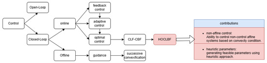
Figure 1.
Flowchart representing a control theory overview situated in the general context and explaining the contributions made.
1.2. Organization
The rest of the paper is organized as follows. Section 2 reviews the mathematical background for control Lyapunov and barrier functions. In Section 3, we expand the scope of the CLFs and CBFs beyond control affine systems, suggest a new high-order CLF formulation, synthesize the CLF-CBF approach, and address the potential infeasibility sources using both heuristic and classical approaches. In Section 4, we demonstrate the efficiency of the HOCLBF approach in controlling 6-DOF powered descent, along with numerical simulation results presented in Section 4.1.5. Conclusions and possible future directions of this work are detailed in Section 5.
2. Preliminaries
This section briefly reviews some fundamental definitions of stabilizing control Lyapunov and barrier functions, while we refer the reader to [8,9,10,11,12,13,14,15,16] for a deeper understanding of these concepts. Consider the nonlinear control-affine system:
where f and g are globally Lipschitz, and are the states and control inputs, respectively, constrained in closed sets, with initial condition .
Definition 1
([10,11,12]). A continuous differentiable function is an exponentially stabilizing control Lyapunov function if it is positive, proper, infinitesimally decreasing, and there exists , such that for any solution :
The Lyapunov function yields a feedback controller that exponentially stabilizes and drives the system to the desired output/zero dynamics, with representing the rate of convergence of the solution:
and this controller is equivalent to a min-norm controller that can be solved via a quadratic program, which proved efficient in experimental application [17,18].
Definition 2
([19]). The relative degree of a differentiable function refers to the number of differentiations required to obtain the control input u explicitly shown in the control function.
Since most systems are not first-order in control inputs, we need to ensure stability using the higher-order derivatives of the Lyapunov function. We can infer asymptotic stability by examining up to the third derivative of the Lyapunov function.
Definition 3
([13]). If the function is three times differentiable, and there exist such that:
then is an asymptotic stabilizing Lyapunov function.
In addition to stability requirements, the nonlinear system (1) is often subject to critical safety measures. These safety measures can be stated as a set C defined by some continuous function as:
where is the boundary of the set representing the critical safety limits, and is the interior of the set constituting all the permissible/safe states. We can use control barrier functions to ensure the solutions will not leave the safe set C, [20]. The CBF is a new mathematical technique used to guarantee the safety and stability of a dynamic system while achieving the desired goals. CBFs are scalar functions that quantify the system’s safety in the current state. The control law is then designed to keep the system within the safety region defined by the CBFs. Mathematically, consider the nonlinear control affine system (1).
Definition 4
([12]). If there exists a continuous function that is strictly increasing and , then α belongs to the extended class functions.
Definition 5
([12]). The function is a zeroing barrier function for the safe set if there exists an extended class function such that:
The existence of the CBF renders the set C forward invariant.
In the same way as Lyapunov functions, control barrier functions require that the control input u appears in . In [16], they propose a higher-order CBF to handle higher-relative-order constraints.
Definition 6
([16]). For the nonlinear system (1) with the differentiable constraint , we define a sequence of functions starting from and a sequence of safe sets associated with each , with :
The function is a high-order control barrier function if there exist extended class functions such that:
, under the condition that .
Ensuring guarantees the forward invariance of the set and, subsequently, the forward invariance of all the sets , hence ensuring the system’s safety within the set , similar to Definition 5. To guarantee the feasibility of the HOCBF, the authors of [16] suggested multiplying the class functions by a penalty term and solving iteratively to relax the problem when needed:
3. A QP Formulation Based on High-Order Control Lyapunov–Barrier Functions
In this section, we synthesize HOCLFs and HOCBFs to control nonlinear systems. We first establish some conditions to extend the use of CLFs and CBFs for controlling and constraining non-affine nonlinear systems. Next, we propose a new form for higher-order CLFs inspired by the analytical first-order CLF in [10,11,12], explicitly displaying the rate of convergence and the computational high-order CLF proposed in [13] incorporating the higher-order derivative of the Lyapunov function. Finally, we suggest a classical controller to address the contrast between the CLFs and a heuristic approach to handle the infeasibility in the QP arising from CLF and CBF conflicts.
Starting from the first formulation of Lyapunov functions [8], Artstein’s theorem considers a general dynamic system of the form and argues its global asymptotic stability under the condition of finding a continuous function such that:
A smooth mapping is constructed to achieve the global asymptotic stability of the system with the feedback law , where belongs to a convex set and U is a convex polytope . It is also suggested to consider a piece-wise linear function to ensure Lipschitz continuity and guarantee the existence of a control law . The linearity in input was further established in the work conducted in [9], where a universal Artstein theorem is constructed for systems with affine inputs. Since Artstein’s theorem guarantees the stability of a general dynamic system, we argue that we can use analytical Lyapunov and barrier functions to stabilize non-affine nonlinear systems using convex optimization under certain conditions.
In this work, we consider a general dynamic system of the form:
where and are the states and control inputs, respectively. f and g are globally Lipschitz, and g is at least twice differentiable. We also consider a continuously differentiable positive-definite function to be an exponentially stabilizing control Lyapunov function yielding the following controller:
Theorem 1.
For a general Lyapunov function , the min-norm controller (13) is a convex quadratic program if is convex, requiring that and are both convex and positive functions (or concave and negative) and have the same monotonicity. Since is a function of the states only, it is sufficient that . That is, is positive and is convex (or negative and concave) in , respectively.
Proof.
We prove the first statement by verifying Jensen’s inequality for the product . If and are positive, convex, and have the same monotonicity, then for , we find:
We prove the second statement by verifying the second-order convexity condition. Taking the first derivative of with respect to the control input eliminates and yields
Taking the second derivative yields
and canceling the term involving , we obtain
Therefore, the convexity of the feasible set in the quadratic program depends on the sign of . □
Remark 1.
With similar reasoning, we can prove that the CBF in (7) defines a convex feasible set for the quadratic program if .
Remark 2.
A control affine system is a special case as .
Example 1.
The following example demonstrates an extreme case where both change sign within while keeping the convexity condition valid. Consider the system
We can drive and stabilize this system from an arbitrary to the unstable equilibrium point at by using the Lyapunov function . This results in
By examining and , we can see a change of sign between and ; nevertheless, for . Hence, we conclude controllability via the control Lyapunov function
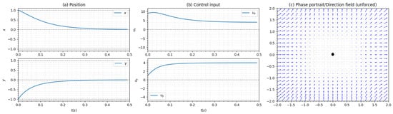
Figure 2 shows the state trajectory, control trajectory, and phase portrait of the unforced system.
Figure 2.
(a) The state trajectory starting from and reaching for . (b) The control trajectory driving the system to . (c) The phase portrait of the unforced system, with blue arrows indicating the existence of an unstable equilibrium point in .
Next, we propose a new computationally efficient form for higher-order CLFs that can exponentially stabilize nonlinear systems. Starting from the HOCLF proposed in [13], we ensure the satisfaction of positiveness and zero dynamics by the initial choice of the Lyapunov function, e.g., taking a quadratic function of the difference between the desired and actual solution guarantees and .
We also omit the scalars and add the Lyapunov function multiplied by a scalar c that represents the rate of convergence of the CLF to the sum of Lyapunov derivatives and obtain the following HOCLF:
Combining high-order Lyapunov and barrier functions can often encounter infeasibilities. The first source of infeasibility comes from the conflicts of goals between the CLFs and CBFs. This problem was overcome in [11,12,21] by adding a relaxing (softening) term to the CLFs, which allows them to diverge from the desired states to guarantee the satisfaction of CBF constraints. The second infeasibility arises from the HOCLF and HOCBF coefficients when their constraints conflict with the constraint of the control input bounds. Although [16] suggested an iterative approach to change the parameters until they make the QP feasible, it relaxes the safety constraints and has a marginally incremental impact on computation time and power. Alternatively, we adopt a heuristic approach where the quadratic program solves for approximate solutions when an optimal solution is impractical or impossible to find, and this is achieved by maximizing the rates of convergence for the CLF and the Kappa function coefficients with a tunable upper bound while minimizing the relaxing terms for the CLF. The last infeasibility to overcome stems from conflicts between the multiple goals of CLFs; e.g., a position CLF driving the system towards a desired position conflicts with the velocity CLF trying to attenuate the velocity to zero, resulting in a quadratic program infeasibility. To overcome this issue, we suggest using state-varying desired states. In other words, instead of using the final desired states in the CLFs, we compute intermediate desired states between the initial and final states. We suggest two methods for determining intermediate states.
Navigational Planner: We can use a navigation algorithm between the initial and final states and obtain a sequence of plausible intermediate states; nonetheless, this method has some distinctive drawbacks. Employing the navigation algorithm offline leaves it myopic to the current state and trajectory; therefore, its intermediate states can become unreachable as the current trajectory progresses, especially for highly nonlinear coupled dynamics. On the other hand, using the algorithm online can generate excellent intermediate states; however, it requires significantly higher computational power and time.
PID Planner: We can use an online PID planner to generate the subsequent intermediary desired state based on our current and final state. We can define the error between the current and final state as , yielding a PID planner as follows:
where are tunable parameters. We adopt this approach in our work as it provides an exceptional compromise between generating online, plausible, reachable intermediate states and considerable computational efficacy. The final form of the optimal quadratic program controller we suggest is as follows:
where are weighing coefficients used to tune the system’s behavior.
4. Simulations and Results
4.1. 6-DOF Optimal Powered Descent
To demonstrate the proposed HOCLBF framework on a more complex system, we address the problem of controlling a 6-DOF powered descent. The model we use in this paper is inspired by [7,22,23] but tailored to accommodate our application. In our model, we assume a single 2D gimbal engine that can continuously vary between minimum and maximum thrusts; the rocket is a rigid body with a constant CG and inertia and we neglect any deformations. We assume the dynamics are mainly governed by inertial and thrust forces and neglect aerodynamic forces based on the findings of [7]. Lastly, we ignore planetary motion and assume a constant gravity throughout the rocket trajectory.
4.1.1. Dynamic Model
To fully describe the dynamics of the 6-DOF rocket, similar to [7,23] we assume the fuel dynamics are governed by an affine function of the thrust magnitude and neglect the atmospheric back pressure:
where . is the vacuum specific impulse of the engine, and is standard Earth gravity. We describe the translational and rotational dynamics with six differential equations as follows.
We add the second derivative of the position and attitude in the inertial frame. We make these adjustments to accommodate the Lyapunov approach efficiently.
4.1.2. High-Order Control Lyapunov Functions
To drive the states to the desired ones, we need to formulate positive Lyapunov functions that are twice differentiable as the order of the position dynamics is . Hence, we use the following quadratic Lyapunov function which satisfies positiveness and the zero dynamics point and yields:
Formulating all the Lyapunov functions with the relaxing terms and PID planner ensures convergence to the desired states while maintaining flexibility to diverge when a conflict of goals happens based on the weights of the relaxing terms. Now that smooth convergence is guaranteed, it is crucial to maintain the states within their designated safe spaces, as described by the safety constraints. This is accomplished through implementing control barrier functions without relaxation to enforce forward invariance for the safe sets.
4.1.3. Safety Constraints
To ensure the safety of the descent, we need to ensure the satisfaction of several non-convex constraints; we start by setting a lower bound on the vehicle mass:
We also want the rocket to stay inside a glide slope cone with half angle and an origin that coincides with the inertial frame:
where and .
To constrain the angular velocities of the rocket, we set an upper bound :
Since there are physical limitations on the controls, we need to set upper and lower bounds on the thrust generated by the engine and ensure that the thrust remains within a gimbal angle dictated by the engine:
Next, we can specify different boundary conditions reflecting several scenarios for our rocket trajectory. We start from a specified initial rocket mass, position, velocity, and angular velocity:
and we aim to control the rocket to satisfy the desired final conditions:
4.1.4. Safety Constraints as Control Barrier Functions
In this section, we formulate a set of first-order and second-order zeroing control barrier functions to confine the system’s states within the designated safe sets. We define the extended class function as a linear function of the safety function itself with a coefficient of 1, as it will be multiplied by an optimized parameter to ensure feasibility. Formulating the highest order CBF yields:
The last step for the barrier functions is replacing the sum and multiplications of parameters and with single parameters , respectively. That is to keep the barrier functions convex in parameters too, enabling the optimization of the parameters inside the quadratic program. Algorithm 1 summarizes the HOCLBF method of solving a sequence of online convex quadratic programs to control the optimal 6-DOF powered descent in real-time. Model parameters were taken from [7,22,23], with additional parameters either manually tuned or heuristically optimized to ensure adequate performance. Note that we strongly suggest using an adaptive fourth Runge-Kutta for time integration to minimize higher-order truncation errors.
| Algorithm 1 HOCLBF for 6-DOF powered descent control. |
|
4.1.5. Numerical Results
In this section, we assess the performance of the HOCLBF in comparison to the base CLF-CBF and the successive convexification approach. Our goal is to demonstrate the advantage of using the HOCLBF in generating feasible solutions compared to the base CLF-CBF with constant parameters, as well as compare its trajectory to the robust SC algorithm. The comparison is carried out under the condition that all other parameters are kept identical to ensure a consistent assessment. We run our algorithm on a standard laptop using a commercial solver “ECOS” [24] suited for embedded applications and obtain an average runtime of less than 1.1 ms. We start by comparing the high-velocity entry and landing between the three approaches, starting from and landing on a circular pad in the presence of a 60° glide slope constraint. In Figure 3, we can see that the base CLF-CBF generates infeasible solutions as soon as it gets closer to the glide slope constraint, while the HOCLBF managed to reach the landing site successfully. We can also see some fluctuations in the HOCLBF compared to the smooth SC trajectory.
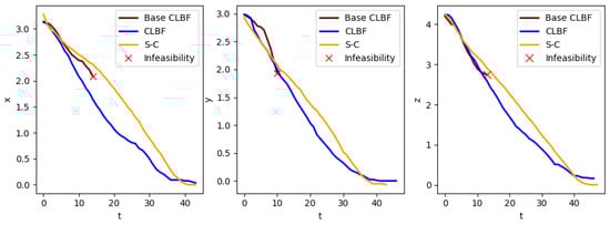
Figure 3.
Trajectory comparison between base CLBF, HOCLBF, and successive convexification with a 60° glide slope constraint. The red ‘x’ marks solution infeasibility.
Figure 4 illustrates the 3D trajectories where we can see that the HOCLBF reaches the landing site successfully, while the base CLF-CBF faces infeasibilities arising from the fixed parameters.
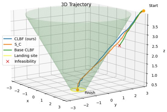
Figure 4.
Three-dimensional trajectory comparison between base CLBF, HOCLBF, and successive convexification with a 60° glide slope constraint.
To demonstrate the efficiency of the CBF approach in ensuring the safety of the rocket landing, we generated a trajectory with no glide slope , then for (Figure 5). For the tighter glide slopes, we can see that despite starting outside the safe region, the rocket moves horizontally at a slower descent rate until it enters the safe region and then starts descending faster and successfully reaches the landing site with no infeasibilities in the QP while keeping the safety constraints satisfied.
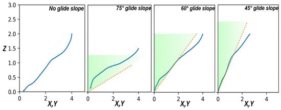
Figure 5.
Trajectories for different glide slope angles in blue; The orange dotted line with the green region illustrates the safe area within the prescribed cone.
4.1.6. Limitations and Future Work
In this work, we attempt to generalize the use of high-order CLFs and CBFs to a wider set of problems and demonstrate the potential of HOCLBFs in safely controlling complex high-dimensional problems. In this work, we overcome the infeasibility issues that arise from the coupling of CLFs and CBFs by using heuristic parameters and we obtain successful results comparable to the robust successive convexification algorithm. Nonetheless, this approach still requires adequate analytical design for the Lyapunov and barrier functions, and some parameters still need initial tuning and are prone to diverge in the presence of high disturbances. Therefore, our next goal is to incorporate some machine learning algorithms alongside differentiable optimization to enhance the performance of the HOCLBF and make it robust to parameter tuning and environmental disturbances.
5. Conclusions
In this paper, we generalize control Lyapunov and barrier functions to general nonlinear dynamic systems with convex input under some conditions and suggest a new formulation of the higher-order control Lyapunov function that guarantees convergence for higher-order dynamics. We unite control Lyapunov and barrier functions using a heuristic approach and an online PID planner ensuring the feasibility of the Quadratic Program. We showcase the efficacy of our HOCLBF approach by devising a real-time six-degree-of-freedom powered descent controller as a convex Quadratic Program. Simulation results for different maneuvers under different safety settings were presented to demonstrate the effectiveness of the HOCLBF in controlling a highly nonlinear coupled system while maintaining safety. In this work, we overcome the infeasibility issues that arise from the coupling of CLFs and CBFs by using heuristic parameters, and we obtain successful results comparable to the robust successive convexification algorithm. Nonetheless, this approach still requires an adequate analytical design for the Lyapunov and barrier functions; some parameters still need initial tuning and are prone to diverge in the presence of high disturbances. Therefore, The next phase of this research will focus on leveraging differentiable convex optimization and reinforcement learning approaches to achieve automatic parameter tuning and intelligent safety constraints. We are also looking into distributional robust optimization to make the HOCLBF robust to model uncertainty and environmental disturbances.
Author Contributions
Conceptualization, methodology, writing, A.E.C. and C.S.; formal analysis, software, validation, visualization, writing—original draft preparation, A.E.C.; supervision, project administration, writing—review and editing, C.S. All authors have read and agreed to the published version of the manuscript.
Funding
This research received no external funding.
Data Availability Statement
All data can be simulated and reproduced from our dynamics models and control algorithms.
Conflicts of Interest
The authors declare no conflicts of interest.
References
- Allgower, F.; Findeisen, R.; Nagy, Z.K. Nonlinear model predictive control: From theory to application. J.-Chin. Inst. Chem. Eng. 2004, 35, 299–316. [Google Scholar]
- Findeisen, R.; Allgöwer, F. An introduction to nonlinear model predictive control. In Proceedings of the 21st Benelux Meeting on Systems and Control, Veldhoven, The Netherlands, 19–21 March 2002; Volume 11, pp. 119–141. [Google Scholar]
- Åström, K.J. Adaptive control. In Mathematical System Theory: The Influence of RE Kalman; Springer: Berlin/Heidelberg, Germany, 1995; pp. 437–450. [Google Scholar]
- Tao, G. Adaptive Control Design and Analysis; John Wiley & Sons: Hoboken, NJ, USA, 2003; Volume 37. [Google Scholar]
- Acikmese, B.; Ploen, S.R. Convex programming approach to powered descent guidance for mars landing. J. Guid. Control. Dyn. 2007, 30, 1353–1366. [Google Scholar] [CrossRef]
- Mao, Y.; Dueri, D.; Szmuk, M.; Açıkmeşe, B. Successive convexification of non-convex optimal control problems with state constraints. IFAC-PapersOnLine 2017, 50, 4063–4069. [Google Scholar] [CrossRef]
- Szmuk, M.; Reynolds, T.P.; Açıkmeşe, B. Successive convexification for real-time six-degree-of-freedom powered descent guidance with state-triggered constraints. J. Guid. Control Dyn. 2020, 43, 1399–1413. [Google Scholar] [CrossRef]
- Artstein, Z. Stabilization with relaxed controls. Nonlinear Anal. Theory Methods Appl. 1983, 7, 1163–1173. [Google Scholar] [CrossRef]
- Sontag, E.D. A ‘universal construction of Artstein’s theorem on nonlinear stabilization. Syst. Control Lett. 1989, 13, 117–123. [Google Scholar] [CrossRef]
- Sontag, E.D. Control-lyapunov functions. In Open problems in Mathematical Systems and Control Theory; Springer: Berlin/Heidelberg, Germany, 1999; pp. 211–216. [Google Scholar]
- Ames, A.D.; Grizzle, J.W.; Tabuada, P. Control barrier function based quadratic programs with application to adaptive cruise control. In Proceedings of the 53rd IEEE Conference on Decision and Control, Los Angeles, CA, USA, 15–17 December 2014; IEEE: Piscataway, NJ, USA, 2014; pp. 6271–6278. [Google Scholar]
- Ames, A.D.; Xu, X.; Grizzle, J.W.; Tabuada, P. Control barrier function based quadratic programs for safety critical systems. IEEE Trans. Autom. Control 2016, 62, 3861–3876. [Google Scholar] [CrossRef]
- Butz, A. Higher order derivatives of Lyapunov functions. IEEE Trans. Autom. Control 1969, 14, 111–112. [Google Scholar] [CrossRef]
- Ahmadi, A.A.; Parrilo, P.A. On higher order derivatives of Lyapunov functions. In Proceedings of the 2011 American Control Conference, San Francisco, CA, USA, 29 June–1 July 2011; IEEE: Piscataway, NJ, USA, 2011; pp. 1313–1314. [Google Scholar]
- Xiao, W.; Belta, C. Control barrier functions for systems with high relative degree. In Proceedings of the 2019 IEEE 58th Conference on Decision and Control (CDC), Nice, France, 11–13 December 2019; IEEE: Piscataway, NJ, USA, 2019; pp. 474–479. [Google Scholar]
- Xiao, W.; Belta, C. High-Order Control Barrier Functions. IEEE Trans. Autom. Control 2022, 67, 3655–3662. [Google Scholar] [CrossRef]
- Mehra, A.; Ma, W.L.; Berg, F.; Tabuada, P.; Grizzle, J.W.; Ames, A.D. Adaptive cruise control: Experimental validation of advanced controllers on scale-model cars. In Proceedings of the 2015 American Control Conference (ACC), Chicago, IL, USA, 1–3 July 2015; IEEE: Piscataway, NJ, USA, 2015; pp. 1411–1418. [Google Scholar]
- Ames, A.D.; Powell, M. Towards the unification of locomotion and manipulation through control lyapunov functions and quadratic programs. In Control of Cyber-Physical Systems; Springer: Berlin/Heidelberg, Germany, 2013; pp. 219–240. [Google Scholar]
- Khalil, H. Nonlinear Systems; Prentice Hall: Hoboken, NJ, USA, 2002. [Google Scholar]
- Blanchini, F. Set invariance in control. Automatica 1999, 35, 1747–1767. [Google Scholar] [CrossRef]
- Romdlony, M.Z.; Jayawardhana, B. Uniting control Lyapunov and control barrier functions. In Proceedings of the 53rd IEEE Conference on Decision and Control, Los Angeles, CA, USA, 15–17 December 2014; IEEE: Piscataway, NJ, USA, 2014; pp. 2293–2298. [Google Scholar]
- Lee, U.; Mesbahi, M. Optimal power descent guidance with 6-DoF line of sight constraints via unit dual quaternions. In Proceedings of the AIAA Guidance, Navigation, and Control Conference, Kissimmee, FL, USA, 5–9 January 2015; p. 0319. [Google Scholar]
- Lee, U.; Mesbahi, M. Dual quaternions, rigid body mechanics, and powered-descent guidance. In Proceedings of the 2012 IEEE 51st IEEE Conference on Decision and Control (CDC), Maui, HI, USA, 10–13 December 2012; IEEE: Piscataway, NJ, USA, 2012; pp. 3386–3391. [Google Scholar]
- Domahidi, A.; Chu, E.; Boyd, S. ECOS: An SOCP solver for embedded systems. In Proceedings of the 2013 European Control Conference (ECC), Zurich, Switzerland, 17–19 July 2013; IEEE: Piscataway, NJ, USA, 2013; pp. 3071–3076. [Google Scholar]
Disclaimer/Publisher’s Note: The statements, opinions and data contained in all publications are solely those of the individual author(s) and contributor(s) and not of MDPI and/or the editor(s). MDPI and/or the editor(s) disclaim responsibility for any injury to people or property resulting from any ideas, methods, instructions or products referred to in the content. |
© 2024 by the authors. Licensee MDPI, Basel, Switzerland. This article is an open access article distributed under the terms and conditions of the Creative Commons Attribution (CC BY) license (https://creativecommons.org/licenses/by/4.0/).