Computing the COVID-19 Basic and Effective Reproduction Numbers Using Actual Data: SEIRS Model with Vaccination and Hospitalization

Abstract

A novel time-dependent deterministic SEIRS model, extended with vaccination, hospitalization, and vital dynamics, is introduced. Time-varying basic and effective reproduction numbers associated with this model are defined, which are crucial metrics in understanding epidemic dynamics. Furthermore, a parameter identification approach has been used to develop a numerical method to compute these numbers for long-term epidemics. We analyze the actual COVID-19 data from the USA, Italy, and Bulgaria to solve appropriate inverse problems and gain an understanding of the time evolution behavior of the basic and effective reproduction numbers. Moreover, an insightful comparison of key coronavirus data and epidemiological parameters across these countries has been conducted. For this purpose, while the basic and effective reproduction numbers provide insights into the virus transmission potential, we propose data-driven criteria for assessing the actual realization of the transmission potential of the SARS-CoV-2 virus and the effectiveness of the applied restrictive measures. To obtain these results, we conduct a mathematical analysis to demonstrate various biological properties of the new differential model, including non-negativity, boundedness, existence, and uniqueness of the solution. The new model and the associated numerical simulation tools proposed herein could be applied to COVID-19 data in any country worldwide and hold a promising potential for the transmission capacity and impact of the virus.

1. Introduction

The COVID-19 pandemic, caused by the SARS-CoV-2 coronavirus, first emerged in Wuhan, Hubei province, China, in December 2019. What initially appeared to be a localized outbreak evolved into a global phenomenon, leading to four major waves over the subsequent three years. By 1 September 2024, according to actual data reported by the World Health Organization (WHO) [1], the pandemic has caused 776,137,815 confirmed cases and 7,061,330 deaths worldwide. To ensure consistency in the interpretation of terms throughout the work, we would like to remark that, in the context of this paper, “actual data” refers specifically to the officially reported data from the referenced sources [2,3,4,5,6,7,8]. By the same timeframe, the global administration of COVID-19 vaccine doses has surpassed 13.64 billion (see [1]), but despite the widespread vaccination efforts and social-distancing measures, the pandemic has been marked by significant morbidity, mortality, and high rates of hospital and intensive care units (ICU) admissions. Related to that, lots of scientists around the world have concentrated their efforts not only on developing effective vaccines and treatment methods, but also on modeling, predicting, and controlling the spread of the virus. In this context, mathematical models serve as a powerful tool for comprehensively modeling virus transmission dynamics, computing crucial epidemiological parameters, and assessing the effectiveness of various methods and measures.

One such parameter is the basic reproduction number ${\Re }_0$, which is a numerical indicator for the transmission potential of the virus. It is defined as the average number of secondary infections produced when one infectious individual is introduced into a completely susceptible host population (see Hethcote [9]). However, the task of defining, calculating, and applying ${\Re }_0$ is by no means trivial and involves certain complexities. In general, ${\Re }_0$ provides information for the herd immunity threshold, which can be used, for example, to estimate the proportion of a given population that must be vaccinated so that the infection is eliminated from that population [10]. When it is not the entire population that is susceptible, a more accurate indicator of the rate of spread of the virus can be utilized, which is the so-called effective reproduction number ${\Re }_e=s{\Re }_0$, where s is the fraction of the host population that is susceptible [11].

Of course, these potential transmission ratios will be reached under the hypothesis that no preventive measures are taken to limit the spread of the virus and that each infectious person moves freely among susceptible individuals. In fact, the officially reported data for daily values of new active (infected) cases and Nonhospitalized active cases since the beginning of the pandemic shows a significantly lower transmission ratio. This allows us to compare the potential and actual transmission ratios of the virus in order to assess the effectiveness of the implemented restrictive measures.

There exist two different types of mathematical models that can be used for simulating epidemic dynamics and computing the basic reproduction number—deterministic and stochastic (see the comparisons in [12,13,14]). Both approaches are commonly applied to estimate and predict the COVID-19 reproduction rates. As a further exploration of these widely utilized methods, in this paper, we consider a deterministic model that is formulated by a Cauchy problem for a system of nonlinear ordinary differential equations.

The first model of this kind is the SIR (Susceptible-Infectious-Recovered) model introduced by Kermack and McKendrick [15], established as a generalization of the classical Lotka-Volterra model. Furthermore, various extended models have been developed based on the SIR/SEIR framework (with E representing the exposed population). A large number of these models have been applied to COVID-19 data in different countries. The various extensions that have been utilized include one or more of the following categories: vital dynamics [16,17], symptomatic and asymptotic infected [18,19], quarantine [16,20], migration [21], vaccination [16,17,22,23], hospitalization and intensive care units [24,25,26]. Several parameter identification approaches have been employed to compute the basic and effective reproduction numbers, typically using classical models such as the inverse problem approach, based on the least squares method for estimation of the SIR model parameters [27,28]; the SIR and SEIR meta-population models [29]; the SEIR model with a hyperbolic tangent form of ${\Re }_e$ [30], or the SEIR model and a Bayesian inference framework [31]; approximations of the solution of SIR model [32].

In the current work, we present a methodology for computing the time behavior of the basic ${\Re }_0$ and effective ${\Re }_e$ reproduction numbers by implementing a novel deterministic model, termed SEIRS-VBHC (SEIRS-VB model, studied in [33,34] extended with hospitalization and ICU), along with its appropriate time-discrete variant. Mathematical analysis of the differential model is carried out in Section 2 and Section 3, while mathematical analysis of the discrete model and numerical experiments are conducted in Section 4 and Section 5. More precisely, the rest of the paper is organized as follows: In Section 2, the novel SEIRS-VBHC model is introduced, and its biological reasonable properties are studied. Using the next-generation method, in Section 3, the basic and effective reproduction numbers associated with the SEIRS-VBHC model are defined. In Section 4, an appropriate time-discrete variant of the model is presented. An inverse problem is formulated and solved for identification of the parameters in the model and computation of ${\Re }_0$ and ${\Re }_e$. Let us mention that usually, the inverse problems are ill-posed. Numerical experiments, using officially available data for COVID-19 in the USA, Italy, and Bulgaria, are conducted in Section 5. The obtained values of the reproduction numbers are compared with the results reported by other authors. As an important epidemiological indicator connected with the official reported data, we defined the actual transmission ratio $T_r =$ New active cases/Nonhospitalized active cases. Seeking some validation of the model SEIRS-VBHC with real data, the time behavior of ${\Re }_e$ and $T_r$ is compared for all three countries. Following other authors, $T_r$ is scaled by different factors for each country. Note that the comparison of the behavior of ${\Re }_e$ and scaled $T_r$ in Section 5 shows that they are very close in every one of all three countries. It is established that the intervals of monotonicity of $T_r$ and scaled ${\Re }_e$ coincide. In the Section 6, the ratio between $T_r$ and ${\Re }_e$ is considered to be an indicator of the realization of the virus’ transmission potential in each of the examined countries. Conclusions are outlined in Section 7.

Let us point out that the proposed epidemiological model SEIRS-VBHC encompasses the main population groups for which officially reported COVID-19 data exists. That is why it is an effective tool for the precise calculation of a range of epidemiological parameters, including the basic and effective reproduction numbers. In order to do this, in the present paper, a non-standard inverse problem is studied. The presented algorithm for solving this problem and determining the parameters in the model gives biologically reasonable results in a real-life situation when applied to the actual COVID-19 data of the USA, Italy, and Bulgaria. The results of the conducted numerical experiments demonstrate that the latter reproduction numbers can be applied to make a credible prognosis for the peaks of new active cases at two-week intervals. In addition, a net new criterion has been developed for both evaluating the realization of the virus’ transmission potential and assessing the effectiveness of the restrictive measure for its spread. The outlined analysis displays a strong correlation between the realization of the virus’ transmission potential and the vaccination and mortality rates reported for the studied countries.

2. The Epidemic Spreading Model SEIRS-VBHC and Its Main Properties

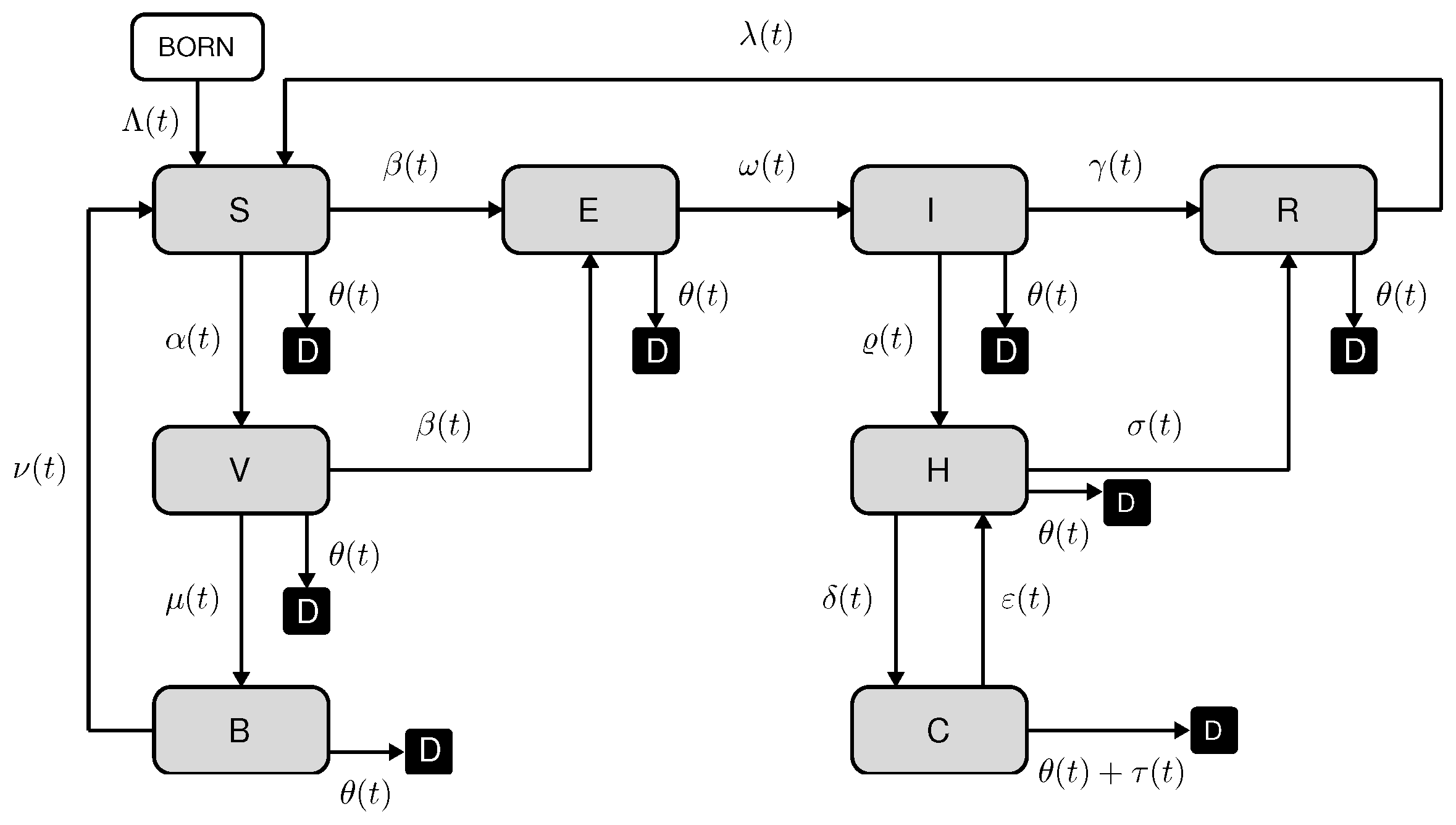
In this section, we present an enhanced SEIRS model that incorporates vaccination, hospitalization, intensive care units, and vital dynamics. Building upon the classical SEIRS framework, which includes the following compartments, Susceptible (S), Exposed (E), Infectious (I), and Recovered (R), the new SEIRS-VBHC model introduces four additional compartments: Vaccinated Susceptible (V), referring to individuals who have been vaccinated but remain susceptible to infection for a short time until they develop antibodies; Individuals with vaccination-acquired immunity (B) describe the group of those who have developed antibodies as a result of vaccination and are protected; Hospitalized Non-Critical (H) represents infectious individuals who are hospitalized but in non-critical condition; Critical (C) refers to individuals in intensive care due to severe infection. This model can also be viewed as an extension of the SEIRS-VB model, which includes the groups H and C. The SEIRS-VB model was introduced and studied in [33,34].

The novel SEIRS-VBHC model has been developed to study the transmission dynamics of COVID-19 using the available officially reported data for important population groups, including hospitalized and individuals in ICU. This enables a more accurate assessment of essential epidemiological parameters, such as the basic and effective reproduction numbers. The SEIRS-VBHC model assumes that all newborn individuals are susceptible and that all individuals who die from the disease have been hospitalized and have passed away in the ICU. In the diagram presented in Figure 1, all individuals who have died, whether from natural causes or the disease, are categorized as group D. It is important to note that deceased individuals are not explicitly included in the model, which focuses on the dynamics of living individuals.

The diagram (Figure 1) illustrates the direction of movement of individuals through the SEIRS-VBHC model compartments by means of the following non-negative parameters:

• $\mathrm{\Lambda }\left(t\right)$—birth rate (newborn/population per unit of time);
• $a\left(t\right)$—vaccination rate (vaccinated/population per unit of time);
• $\phi \left(t\right)$—vaccine effectiveness (excess risk/risk among vaccinated);
• $\alpha \left(t\right)=a\left(t\right)\phi \left(t\right)$—vaccination parameter;
• $\beta \left(t\right)$—transmission rate—average number of adequate contacts (i.e., contacts sufficient for transmission) of a person per unit time (see [9]);
• $\gamma \left(t\right)$—recovery rate of non-hospitalized individuals (1/time);
• $\omega \left(t\right)$—latency rate (1/time);
• $\theta \left(t\right)$—natural mortality rate (new deaths/population per unit of time);
• $\tau \left(t\right)$—mortality rate of infectious people (new deaths/infectious per unit of time);
• $\lambda \left(t\right)$—reinfection rate of recovered individuals (1/time);
• $\nu \left(t\right)$—reinfection rate of vaccinated individuals (1/time);
• $\mu \left(t\right)$—antibody rate (1/time);
• $\varrho \left(t\right)$—hospitalization rate (new hospitalized/infectious per unit of time);
• $\sigma \left(t\right)$—recovery rate of hospitalized individuals (1/time);
• $\delta \left(t\right)$— ICU rate (new ICU /hospitalized per unit of time);
• $\epsilon \left(t\right)$—rehospitalization rate of patients in the ICU (rehospitalized/ICU per unit of time).

The model is described mathematically by the following system of nonlinear ordinary differential equations:

$$\begin{array}{c}{\displaystyle \frac{dS}{dt}}=-\left[\alpha \left(t\right)+\theta \left(t\right)+{\displaystyle \frac{\beta \left(t\right)}{N\left(t\right)}}I\left(t\right)\right]S\left(t\right)+\mathrm{\Lambda }\left(t\right)N\left(t\right)+\lambda \left(t\right)R\left(t\right)+\nu \left(t\right)B\left(t\right),\hfill \\ \\ {\displaystyle \frac{dE}{dt}}=-[\omega \left(t\right)+\theta \left(t\right)]E\left(t\right)+{\displaystyle \frac{\beta \left(t\right)}{N\left(t\right)}}[S\left(t\right)+V\left(t\right)]I\left(t\right),\hfill \\ \\ {\displaystyle \frac{dI}{dt}}=-[\gamma \left(t\right)+\varrho \left(t\right)+\theta \left(t\right)]I\left(t\right)+\omega \left(t\right)E\left(t\right),\hfill \\ \\ {\displaystyle \frac{dR}{dt}}=-[\lambda \left(t\right)+\theta \left(t\right)]R\left(t\right)+\gamma \left(t\right)I\left(t\right)+\sigma \left(t\right)H\left(t\right),\hfill \\ \\ {\displaystyle \frac{dV}{dt}}=-\left[\mu \left(t\right)+\theta \left(t\right)+{\displaystyle \frac{\beta \left(t\right)}{N\left(t\right)}}I\left(t\right)\right]V\left(t\right)+\alpha \left(t\right)S\left(t\right),\hfill \\ \\ {\displaystyle \frac{dB}{dt}}=-[\nu \left(t\right)+\theta \left(t\right)]B\left(t\right)+\mu \left(t\right)V\left(t\right),\hfill \\ \\ {\displaystyle \frac{dH}{dt}}=-[\sigma \left(t\right)+\delta \left(t\right)+\theta \left(t\right)]H\left(t\right)+\varrho \left(t\right)I\left(t\right)+\epsilon \left(t\right)C\left(t\right),\hfill \\ \\ {\displaystyle \frac{dC}{dt}}=-[\epsilon \left(t\right)+\tau \left(t\right)+\theta \left(t\right)]C\left(t\right)+\delta \left(t\right)H\left(t\right),\hfill \end{array}$$

(1)

with non-negative initial conditions

$$\begin{array}{cc}\hfill & S\left(t_0\right)=S_0,E\left(t_0\right)=E_0,I\left(t_0\right)=I_0,R\left(t_0\right)=R_0,\hfill \\ \hfill & V\left(t_0\right)=V_0,B\left(t_0\right)=B_0,H\left(t_0\right)=H_0,C\left(t_0\right)=C_0,\hfill \end{array}$$

(2)

where $t_0,S_0,E_0,R_0,V_0,B_0,H_0,C_0$ are non-negative constants. In the Cauchy problem (1), (2), the population size (the number of all living individuals)

$$N\left(t\right):=S\left(t\right)+E\left(t\right)+I\left(t\right)+R\left(t\right)+V\left(t\right)+B\left(t\right)+H\left(t\right)+C\left(t\right)$$

(3)

is a time-dependent function. Following [33] we introduce the notations

$$X\left(t\right):=\left(S\left(t\right),E\left(t\right),I\left(t\right),R\left(t\right),V\left(t\right),B\left(t\right),H\left(t\right),C\left(t\right)\right),$$

$$X_0:=\left(S_0,E_0,I_0,R_0,V_0,B_0,H_0,C_0\right),$$

and

$$N_0:=N\left(t_0\right)=S_0+E_0+I_0+R_0+V_0+B_0+H_0+C_0.$$

(4)

Remark 1. 

According to the notation here and further, we write that a real vector $x=(x_1,x_2,\dots ,x_n)$ is non-negative/positive if all its components $x_j$ are non-negative/positive. Furthermore, we use $l_1$ norm ${\parallel x\parallel }_1= |x_1|+|x_2|+\dots +|x_n|$.

We intend to apply the new SEIRS-VBHC model to COVID-19 data in different countries. Typically, the official data contain information on the daily (or weekly) number of individuals in different groups related to the model (1) and (2). For this reason, we assume that the parameters in the model SEIRS-VBHC are constant for a certain period of time—a day (or a week), and we consider the following form of system (1) in the case of constant coefficients:

$$\begin{array}{c}{\displaystyle \frac{dS}{dt}}=-\left[\alpha +\theta +bI\left(t\right)\right]S\left(t\right)+\mathrm{\Omega }+\lambda R\left(t\right)+\nu B\left(t\right),\hfill \\ \\ {\displaystyle \frac{dE}{dt}}=-[\omega +\theta ]E\left(t\right)+b[S\left(t\right)+V\left(t\right)]I\left(t\right),\hfill \\ \\ {\displaystyle \frac{dI}{dt}}=-[\gamma +\varrho +\theta ]I\left(t\right)+\omega E\left(t\right),\hfill \\ \\ {\displaystyle \frac{dR}{dt}}=-[\lambda +\theta ]R\left(t\right)+\gamma I\left(t\right)+\sigma H\left(t\right),\hfill \\ \\ {\displaystyle \frac{dV}{dt}}=-\left[\mu +\theta +bI\left(t\right)\right]V\left(t\right)+\alpha S\left(t\right),\hfill \\ \\ {\displaystyle \frac{dB}{dt}}=-[\nu +\theta ]B\left(t\right)+\mu V\left(t\right),\hfill \\ \\ {\displaystyle \frac{dH}{dt}}=-[\sigma +\delta +\theta ]H\left(t\right)+\varrho I\left(t\right)+\epsilon C\left(t\right),\hfill \\ \\ {\displaystyle \frac{dC}{dt}}=-[\epsilon +\tau +\theta ]C\left(t\right)+\delta H\left(t\right),\hfill \end{array}$$

(5)

where the new parameters are

$$\mathrm{\Omega }:=\mathrm{\Lambda }\left(t\right)N\left(t\right),b:={\displaystyle \frac{\beta \left(t\right)}{N\left(t\right)}}.$$

(6)

We suppose that all parameters

$$\begin{array}{c}\hfill p:=(\mathrm{\Omega },\theta ,\omega ,\mu ,\alpha ,b,\gamma ,\tau ,\nu ,\lambda ,\varrho ,\sigma ,\delta ,\epsilon )\end{array}$$

(7)

are positive constants.

We consider a real-life epidemic situation where numbers of susceptible S (at the beginning of the COVID-19 epidemic the entire population is susceptible, i.e., $S_0\approx N_0>0$), infectious I and hospitalized H individuals are positive. That is why a natural candidate for a feasible region of the model (5) and (2) is

$$\mathrm{\Sigma }:=\left\{X=(S,E,I,R,V,B,H,C)\in {\mathbb{R}}^8:X\ge 0,S>0,I>0,H>0,{\parallel X\parallel }_1\le {\displaystyle \frac{\mathrm{\Omega }}{\theta }}\right\}.$$

(8)

Theorem 1. 

Let the initial data $X_0\in \mathrm{\Sigma }$ and all parameters $p>0$ are constants. Then, for each arbitrary but fixed $T>t_0$, there exists a solution $X\left(t\right)$ of the Cauchy problem (5) and (2), which is defined for $t\in [t_0,T]$ and $X\left(t\right)\in \mathrm{\Sigma }$ for $t\in [t_0,T].$ The solution with such properties is unique.

Proof. 

The vector valued function on the right-hand side of the system (5) (which elements are second-order polynomials with respect to X components) is continuous and differentiable in ${\mathbb{R}}^8$. According to Picard’s existence and uniqueness theorem (Theorem 1.1., p. 8 in [35]), there exists a unique solution $X\left(t\right)$ of the Cauchy problem (5) and (2), defined in the interval $[t_0,T_1]$ for some $T_1\in (t_0,T]$. Now, we will show that $T_1=T$.

Step 1. First of all, we prove that $X\left(t\right)\ge 0,S\left(t\right)>0,I\left(t\right)>0,H\left(t\right)>0$ for $t\in [t_0,T_1].$

Since $X_0\in \mathrm{\Sigma }$, we have $S\left(t_0\right)=S_0>0,I\left(t_0\right)=I_0>0$ and $H\left(t_0\right)=H_0>0$. The functions $S\left(t\right),I\left(t\right),H\left(t\right)$ are continuous in $[t_0,T_1]$, and therefore, they are positive at least for t greater than and close enough to $t_0$. Let us assume that $S\left(t\right)I\left(t\right)H\left(t\right)$ vanishes in $(t_0,T_1]$ and denote with $t_1\in (t_0,T_1]$ the first time such that $S\left(t_1\right)I\left(t_1\right)H\left(t_1\right)=0,$ i.e., $S\left(t\right)>0,I\left(t\right)>0$ and $H\left(t\right)>0$ for $t\in [t_0,t_1)$.

We observe that each equation in the system (5) is a linear first-order ODE with respect to one of the components of $X\left(t\right)$. Now, using the initial conditions (2) and taking into account that all parameters in p (see (7)) are positive constants, for $t\in [t_0,t_1]$, we perform the calculations outlined below.

The proof of Theorem 1 is in the spirit of Theorem 1 in our previous publication [33] according to the components of vector $X\left(t\right)$, except $H\left(t\right)$ and $C\left(t\right)$. Thus, we have: $V\left(t\right)\ge 0,R\left(t\right)\ge 0,E\left(t\right)\ge 0,B\left(t\right)\ge 0$ and $S\left(t\right)>0,I\left(t\right)>0$ for $t_0\le t\le t_1$.

Furthermore, from C-equation in (5) with $C_0\ge 0,H\left(t\right)\ge 0$ we calculate

$$C\left(t\right)=e^{(\epsilon +\tau +\theta )(t_0-t)}\left(C_0+\delta {\int }_{t_0}^{t}H\left(z\right)e^{(\epsilon +\tau +\theta )(z-t_0)}dz\right)\ge 0.$$

(9)

Since $H\left(t_1\right)\ge 0$ and $H\left(t\right)>0$ for $t\in [t_0,t_1)$ from (9) we conclude

$$C\left(t_1\right)>0.$$

(10)

Since, $S\left(t_1\right)I\left(t_1\right)>0$ it follows $H\left(t_1\right)=0$. Then H-equation in (5) and (10) give

$${\displaystyle \frac{dH\left(t_1\right)}{dt}}=\epsilon C\left(t_1\right)>0$$

and, because $H\left(t\right)>0$ for $t_0\le t<t_1$, it leads to a contradiction with $H\left(t_1\right)=0$. It follows that $H\left(t\right)>0$ for $t\in [t_0,T_1]$.

Hence, $S\left(t\right)>0,I\left(t\right)>0$, $H\left(t\right)>0$ and other components are non-negative for $t\in [t_0,T_1]$.

Step 2. We prove that ${\parallel X\left(t\right)\parallel }_1\le {\displaystyle \frac{\mathrm{\Omega }}{\theta }}$ for $t\in [t_0,T_1].$

Since $X\left(t\right)\ge 0$ for $t\in [t_0,T_1]$ it follows that ${\parallel X\left(t\right)\parallel }_1=N\left(t\right)$ is the total population size (see (3)). Adding the equations of the system (5) and using the initial conditions (2), we obtain that function $N\left(t\right)$ satisfies the following Cauchy problem:

$$\begin{array}{c}{\displaystyle \frac{dN\left(t\right)}{dt}=\mathrm{\Omega }-\theta N\left(t\right)-\tau C\left(t\right),t_0\le t\le T_1,}\hfill \\ \\ N\left(t_0\right)=N_0.\hfill \end{array}$$

(11)

The unique solution of this linear Cauchy problem is

$$N\left(t\right)={\displaystyle \frac{\mathrm{\Omega }}{\theta }}+\left(N_0-{\displaystyle \frac{\mathrm{\Omega }}{\theta }}\right)e^{\theta (t_0-t)}-\tau e^{-\theta t}{\int }_{t_0}^t{e}^{\theta s}C\left(s\right)ds.$$

(12)

Since $C\left(t\right)>0$ for $t\in [t_0,T_1]$ and $X_0\in \mathrm{\Sigma }$ it follows that $N_0\le \mathrm{\Omega }/\theta$ and therefore $N\left(t\right)\le {\displaystyle \frac{\mathrm{\Omega }}{\theta }}.$ Hence, ${\parallel X\left(t\right)\parallel }_1\le {\displaystyle \frac{\mathrm{\Omega }}{\theta }}$ for $t\in [t_0,T_1]$.

Step 3. We prove that $X\left(t\right)$ is defined for $t\in [t_0,T]$ and $X\left(t\right)\in \mathrm{\Sigma }$ for $t\in [t_0,T].$

From Step 1 and Step 2 it follows that $X\left(t\right)$ is defined for $t\in [t_0,T_1]$ and $X\left(t\right)\in \mathrm{\Sigma }$ for $t\in [t_0,T_1].$ Since ${\parallel X\left(t\right)\parallel }_1\le {\displaystyle \frac{\mathrm{\Omega }}{\theta }}$, the solution is uniformly bounded on $[t_0,T_1]$. Now, by Extension theorem (Theorem 3.1., p. 12 in [35]), we conclude that $T_1\equiv T,$ i.e., the solution $X\left(t\right)$ exists on $[t_0,T]$ and $X\left(t\right)\in \mathrm{\Sigma }$ for $t\in [t_0,T].$

This completes the proof. □

Remark 2. 

Following [33], some existence and uniqueness results, similar to these in Theorem 1, can be obtained in the case of the Cauchy problem (1) and (2) with time-dependent coefficients under some additional conditions.

3. The Basic and Effective Reproduction Numbers, Associated with the SEIRS-VBHC Model

In this section, we introduce the basic reproduction number ${\Re }_0$, associated with the SEIRS-VBHC model in the autonomous case (5). Furthermore, we define the effective reproduction number ${\Re }_e\left(t\right)$ as the product of the basic reproduction number and the fraction of the host population that is susceptible.

The basic reproduction number is a mathematically defined quantity, which measures the transmission potential of the disease, and it correlates to the stability of the equilibrium points of the system (5). The most commonly used way to determine ${\Re }_0$ is the next-generation method (see [36,37]), which is related to study of the disease-free equilibrium points (without infected individuals, i.e., $E=0,I=0,H=0,C=0$) of the system (5). That is why we search for solutions ($S,0,0,R,V,B,0,0$) of the corresponding homogeneous system for equilibrium points of (5). We obtain the system

$$\begin{array}{c}-\left[\alpha +\theta \right]S+\mathrm{\Omega }+\nu B=0,\hfill \\ \\ -\left[\lambda +\theta \right]R=0,\hfill \\ \\ -\left[\mu +\theta \right]V+\alpha S=0,\hfill \\ \\ -[\nu +\theta ]B+\mu V=0.\hfill \end{array}$$

(13)

The system (13) is linear and has a unique solution that implies the following disease-free equilibrium point of (5):

$$\begin{array}{c}\hfill X^{\ast }:=(S^{\ast },E^{\ast },I^{\ast },R^{\ast },V^{\ast },B^{\ast },H^{\ast },C^{\ast })=\left(1,0,0,0,{\displaystyle \frac{\alpha }{\mu +\theta }},{\displaystyle \frac{\alpha \mu }{(\mu +\theta )(\nu +\theta )}},0,0\right)S^{\ast },\end{array}$$

(14)

where

$$S^{\ast }:={\displaystyle \frac{\mathrm{\Omega }(\nu +\theta )(\mu +\theta )}{\theta (\alpha \nu +(\mu +\theta \left)\right(\alpha +\nu +\theta \left)\right)}}>0.$$

To define the basic reproduction number associated with system (5), we are following the next-generation method (see [36]). Since we are concerned with the host populations that spread the infection, according to this method, we need only to consider a reduced model. This model describes the interaction between exposed E, infected I, hospitalized H, and critical C categories. Therefore, it is enough to consider only the subsystem that contains virus carriers $Y=(E,I,H,C)$. The dynamics in these compartments are modeled by the following subsystem of (5):

$$\begin{array}{c}{\displaystyle \frac{dE\left(t\right)}{dt}}=-[\omega +\theta ]E\left(t\right)+b[S\left(t\right)+V\left(t\right)]I\left(t\right),\hfill \\ \\ {\displaystyle \frac{dI\left(t\right)}{dt}}=-[\gamma +\varrho +\theta ]I\left(t\right)+\omega E\left(t\right),\hfill \\ \\ {\displaystyle \frac{dH\left(t\right)}{dt}}=-[\sigma +\delta +\theta ]H\left(t\right)+\varrho I\left(t\right)+\epsilon C\left(t\right),\hfill \\ \\ {\displaystyle \frac{dC\left(t\right)}{dt}}=-[\epsilon +\tau +\theta ]C\left(t\right)+\delta H\left(t\right).\hfill \end{array}$$

(15)

In this case, the basic reproduction number is defined as the spectral radius of the next-generation matrix (operator) for the system (15). For a detailed explanation of the formation of the next-generation matrix and definition of the basic reproduction number, see [36,38] and references therein. Following [34] we obtain the basic reproduction number of (5):

$${\Re }_0:={\displaystyle \frac{\omega b\mathrm{\Omega }(\nu +\theta )(\alpha +\mu +\theta )}{\theta (\omega +\theta )(\gamma +\varrho +\theta )(\alpha \nu +(\mu +\theta \left)\right(\alpha +\nu +\theta \left)\right)}}.$$

(16)

To define the effective reproduction number, we observe that two compartments of the SEIRS-VBHC model involve susceptible individuals—S (unvaccinated and vaccinated for whom the vaccine is not effective) and V (vaccinated for whom the vaccine is effective but they have not yet developed antibodies). Then, the effective reproduction number, associated with the model (5) is defined as the product of the basic reproduction number and the fraction of the host population that is susceptible (see [11]):

$${\Re }_e\left(t\right):={\Re }_0{\displaystyle \frac{S\left(t\right)+V\left(t\right)}{N\left(t\right)}}.$$

(17)

4. Methodology for Computing ${\mathit{R}}_{\mathbf{0}}$ and ${\mathit{R}}_{\mathit{e}}\mathbf{\left(}\mathit{t}\mathbf{\right)}$ Using Actual Data

In this section, we define an algorithm for computation of the daily or weakly values of the basic and effective reproduction numbers, introduced in Section 3. First, we mention that using relations (6) and (16), one can find a representation of the basic reproduction number by parameters of system (1):

$${\Re }_0:={\displaystyle \frac{\omega \beta \mathrm{\Lambda }(\nu +\theta )(\alpha +\mu +\theta )}{\theta (\omega +\theta )(\gamma +\varrho +\theta )(\alpha \nu +(\mu +\theta \left)\right(\alpha +\nu +\theta \left)\right)}}.$$

(18)

In order to be able to use officially reported daily or weekly data on COVID-19, we consider a suitable discrete variant of the differential SEIRS-VBHC model. Following [33], we introduce a semi-implicit difference scheme as a time-discrete analog of the Cauchy problem (1), (2).

We consider a timeframe $t_1,t_2,\dots ,t_K$, where $t_k=t_1+(k-1)h,k=2,3,\dots ,K$ and the size $h>0$. If $h=1day$, then $t_k$ are fixed consecutive days of the epidemic. Furthermore, we introduce the notation for the values of functions

$$\begin{array}{cc}\hfill X_k& :=(S_k,E_k,I_k,R_k,V_k,B_k,H_k,C_k)\hfill \\ & =(S\left(t_k\right),E\left(t_k\right),I\left(t_k\right),R\left(t_k\right),V\left(t_k\right),B\left(t_k\right),H\left(t_k\right),C\left(t_k\right)),\hfill \end{array}$$

$$N_k:=N\left(t_k\right)=S_k+E_k+I_k+R_k+V_k+B_k+H_k+C_k,$$

for $k=1,2,\dots ,K$ and the values of the parameters

$$\begin{array}{cc}\hfill p_k& :=({\alpha }_k,{\beta }_k,{\gamma }_k,{\tau }_k,{\mathrm{\Lambda }}_k,{\theta }_k,{\omega }_k,{\lambda }_k,{\mu }_k,{\nu }_k,{\varrho }_k,{\sigma }_k,{\delta }_k,{\epsilon }_k)\hfill \\ \hfill & =(\alpha \left(t_k\right),\beta \left(t_k\right),\gamma \left(t_k\right),\tau \left(t_k\right),\mathrm{\Lambda }\left(t_k\right),\theta \left(t_k\right),\omega \left(t_k\right),\lambda \left(t_k\right),\mu \left(t_k\right),\nu \left(t_k\right),\hfill \\ \hfill & \varrho \left(t_k\right),\sigma \left(t_k\right),\delta \left(t_k\right),\epsilon \left(t_k\right)),\hfill \end{array}$$

(19)

$k=1,2,\dots ,K-1.$

Remark 3. 

In [34] two-weight family of semi-implicit difference schemes is introduced as time-discrete analogue of the simpler differential model SEIRS-VB. It is shown that a weighted convex linear combination scheme can provide higher accuracy while maintaining stability than the explicit (forward) Euler scheme and implicit (backward) Euler scheme. Keeping these results in mind, we consider the time-discrete analog of the differential SEIRS-VBHC model with weights $1/2$.

Using the initial values $S\left(t_1\right)=S_1,E\left(t_1\right)=E_1,I\left(t_1\right)=I_1,R\left(t_1\right)=R_1,V\left(t_1\right)=V_1,B\left(t_1\right)=B_1,H\left(t_1\right)=H_1,C\left(t_1\right)=C_1$, we consider now the following difference scheme:

$$\begin{array}{cc}\hfill {\displaystyle \frac{S_k-S_{k-1}}{h}}=& -\left[{\alpha }_{k-1}+{\theta }_{k-1}+{\displaystyle \frac{{\beta }_{k-1}}{N_{k-1}}}\left({\displaystyle \frac{1}{2}}{I}_{k-1}+{\displaystyle \frac{1}{2}}{I}_k\right)\right]S_{k-1}+{\mathrm{\Lambda }}_{k-1}{N}_{k-1}\hfill \\ & +{\lambda }_{k-1}{R}_{k-1}+{\nu }_{k-1}{B}_{k-1},\hfill \\ \hfill {\displaystyle \frac{E_k-E_{k-1}}{h}}=& -({\omega }_{k-1}+{\theta }_{k-1})E_{k-1}+{\displaystyle \frac{{\beta }_{k-1}}{N_{k-1}}}(S_{k-1}+V_{k-1})\left({\displaystyle \frac{1}{2}}{I}_{k-1}+{\displaystyle \frac{1}{2}}{I}_k\right),\hfill \\ \hfill {\displaystyle \frac{I_k-I_{k-1}}{h}}=& -({\gamma }_{k-1}+{\varrho }_{k-1})\left({\displaystyle \frac{1}{2}}{I}_{k-1}+{\displaystyle \frac{1}{2}}{I}_k\right)-{\theta }_{k-1}{I}_{k-1}+{\omega }_{k-1}{E}_{k-1},\hfill \\ \hfill {\displaystyle \frac{R_k-R_{k-1}}{h}}=& -({\lambda }_{k-1}+{\theta }_{k-1})R_{k-1}+{\gamma }_{k-1}\left({\displaystyle \frac{1}{2}}{I}_{k-1}+{\displaystyle \frac{1}{2}}{I}_k\right)+{\sigma }_{k-1}{H}_{k-1},\hfill \\ \hfill {\displaystyle \frac{V_k-V_{k-1}}{h}}=& -\left[{\mu }_{k-1}+{\theta }_{k-1}+{\displaystyle \frac{{\beta }_{k-1}}{N_{k-1}}}\left({\displaystyle \frac{1}{2}}{I}_{k-1}+{\displaystyle \frac{1}{2}}{I}_k\right)\right]V_{k-1}+{\alpha }_{k-1}{S}_{k-1},\hfill \\ \hfill {\displaystyle \frac{B_k-B_{k-1}}{h}}=& -({\nu }_{k-1}+{\theta }_{k-1})B_{k-1}+{\mu }_{k-1}{V}_{k-1},\hfill \\ \hfill {\displaystyle \frac{H_k-H_{k-1}}{h}}=& -({\sigma }_{k-1}+{\delta }_{k-1}+{\theta }_{k-1})H_{k-1}+{\varrho }_{k-1}\left({\displaystyle \frac{1}{2}}{I}_{k-1}+{\displaystyle \frac{1}{2}}{I}_k\right)\hfill \\ & +{\epsilon }_{k-1}{C}_{k-1},\hfill \\ \hfill {\displaystyle \frac{C_k-C_{k-1}}{h}}=& -({\epsilon }_{k-1}+{\tau }_{k-1}+{\theta }_{k-1})C_{k-1}+{\delta }_{k-1}{H}_{k-1},\hfill \end{array}$$

(20)

where $k=2,3,\dots ,K$.

Our first objective is to demonstrate that the discrete problem (20), with suitable initial data exhibits biologically reasonable features, similar to those of the differential model (5). Therefore, as a next step, we will find sufficient conditions for the values of parameters $p_k$ (see (19)) and the step size h in the difference scheme (20) which guarantee preserving the component-wise non-negativity of the numerical solution.

Theorem 2. 

Let $X_1\ge 0$ with $S_1>0,I_1>0,H_1>0$, $p_{k-1}\ge 0$ for all $k=2,3,\dots ,K$ and

$$\underset{k=2,\dots ,K}{max}{q}_{k-1}<{\displaystyle \frac{1}{h}}$$

(21)

where

$$\begin{array}{cc}\hfill q_{k-1}:=& {\theta }_{k-1}+max\{{\displaystyle \frac{{\gamma }_{k-1}}{2}}+{\displaystyle \frac{{\rho }_{k-1}}{2}}+{\omega }_{k-1},{\alpha }_{k-1}+{\beta }_{k-1},{\mu }_{k-1}+{\beta }_{k-1},\hfill \\ & {\sigma }_{k-1}+{\delta }_{k-1},{\epsilon }_{k-1}+{\tau }_{k-1},{\nu }_{k-1},{\lambda }_{k-1}\}.\hfill \end{array}$$

Then for the values $X_k=(S_k,E_k,I_k,R_k,V_k,B_k,H_k,C_k)$ obtained by (20), we have that $X_k\ge 0$, $S_k>0,I_k>0$ and $H_k>0$ holds, for all $k=1,2,\dots ,K$.

Proof. 

For $X_1$ the statement of the theorem holds. We suppose that $X_{k-1}\ge 0$ with $S_{k-1}>0,I_{k-1}>0,H_{k-1}>0$ for some $k\in [2,K-1]$. Therefore $I_{k-1}<N_{k-1}$.

We express (20) in the following form:

$$\begin{array}{c}{S}_k=\begin{array}{c}\left[1-h\left({\alpha }_{k-1}+{\theta }_{k-1}+{\displaystyle \frac{{\beta }_{k-1}}{N_{k-1}}}\left({\displaystyle \frac{1}{2}}{I}_{k-1}+{\displaystyle \frac{1}{2}}{I}_k\right)\right)\right]S_{k-1}\hfill \\ +h({\mathrm{\Lambda }}_{k-1}{N}_{k-1}+{\lambda }_{k-1}{R}_{k-1}+{\nu }_{k-1}{B}_{k-1})],\hfill \end{array}\hfill \\ E_k=[1-h({\omega }_{k-1}+{\theta }_{k-1})]E_{k-1}+{\displaystyle \frac{{\beta }_{k-1}}{N_{k-1}}}\left(S_{k-1}+V_{k-1}\right)\left({\displaystyle \frac{1}{2}}{I}_{k-1}+{\displaystyle \frac{1}{2}}{I}_k\right),\hfill \\ I_k={\displaystyle \frac{2-h({\gamma }_{k-1}+{\rho }_{k-1}+2{\theta }_{k-1})}{2+h({\gamma }_{k-1}+{\rho }_{k-1})}}{I}_{k-1}+{\displaystyle \frac{2h{\omega }_{k-1}}{2+h({\gamma }_{k-1}+{\rho }_{k-1})}}{E}_{k-1},\hfill \\ R_k=[1-h({\lambda }_{k-1}+{\theta }_{k-1})]R_{k-1}+h{\gamma }_{k-1}\left({\displaystyle \frac{1}{2}}{I}_{k-1}+{\displaystyle \frac{1}{2}}{I}_k\right)+h{\sigma }_{k-1}{H}_{k-1},\hfill \\ V_k=\left[1-h\left({\mu }_{k-1}+{\theta }_{k-1}+{\displaystyle \frac{{\beta }_{k-1}}{N_{k-1}}}\left({\displaystyle \frac{1}{2}}{I}_{k-1}+{\displaystyle \frac{1}{2}}{I}_k\right)\right)\right]V_{k-1}+h{\alpha }_{k-1}{S}_{k-1},\hfill \\ B_k=[1-h({\nu }_{k-1}+{\theta }_{k-1}]B_{k-1}+h{\mu }_{k-1}{V}_{k-1},\hfill \\ H_k=[1-h({\sigma }_{k-1}+{\delta }_{k-1}+{\theta }_{k-1})]H_{k-1}+h{\rho }_{k-1}\left({\displaystyle \frac{1}{2}}{I}_{k-1}+{\displaystyle \frac{1}{2}}{I}_k\right)+h{\epsilon }_{k-1}{C}_{k-1},\hfill \\ C_k=[1-h({\epsilon }_{k-1}+{\tau }_{k-1}+{\theta }_{k-1})]C_{k-1}+h{\delta }_{k-1}{H}_{k-1}.\hfill \end{array}$$

(22)

Using (21), we carry out the following steps:

• From the I-equation in (22), it follows that

  $$\begin{array}{cc}\hfill I_k& <{\displaystyle \frac{2-h({\gamma }_{k-1}+{\rho }_{k-1}+2{\theta }_{k-1})}{2+h({\gamma }_{k-1}+{\rho }_{k-1})}}(I_{k-1}+E_{k-1})\hfill \\ \hfill & \le {\displaystyle \frac{2-h({\gamma }_{k-1}+{\rho }_{k-1}+2{\theta }_{k-1})}{2+h({\gamma }_{k-1}+{\rho }_{k-1})}}{N}_{k-1}\hfill \\ \hfill & <N_{k-1}.\hfill \end{array}$$

  (23)
  On the other hand, $I_{k-1}>0$ and condition (21) ensures that $2-h({\gamma }_{k-1}+{\rho }_{k-1}+2{\theta }_{k-1})>0$. Hence $I_k>0$.
• Since $S_{k-1}>0$, we now consider the S-equation in (22). By applying (23) and $I_{k-1}<N_{k-1}$, we obtain

  $$\begin{array}{cc}\hfill S_k\ge & [1-h({\alpha }_{k-1}+{\theta }_{k-1}+{\beta }_{k-1})]S_{k-1}\hfill \\ & +h[{\mathrm{\Lambda }}_{k-1}{N}_{k-1}+{\lambda }_{k-1}{R}_{k-1}+{\nu }_{k-1}{B}_{k-1}].\hfill \end{array}$$
  Condition (21) implies $1-h({\alpha }_{k-1}+{\theta }_{k-1}+{\beta }_{k-1})>0$ and we conclude that $S_k>0$.
• By applying (23) and $I_{k-1}<N_{k-1}$ to the E-equation and V-equation in (22) we obtain $E_k\ge 0$ and $V_k\ge 0$. The R-equation, B-equation and C-equation yield $R_k\ge 0$, $B_k\ge 0$, and $C_k\ge 0$, respectively.
• Finally, let us consider H-equation in (22). Condition (21) ensures that the coefficient $1-h({\sigma }_{k-1}+{\delta }_{k-1}+{\theta }_{k-1})>0$. Additionally, by taking into account that $H_{k-1}>0$ we obtain $H_k>0.$

The proof is complete. □

Let us mention that the officially reported data usually contains information for the numbers of individuals in some compartments that do not appear explicitly in the SEIRS-BVHC model:

• $A\left(t\right)=E\left(t\right)+I\left(t\right)+H\left(t\right)+C\left(t\right)$—The number of active cases;
• $Rtotal\left(t\right)$—The cumulative number of individuals recovered from the disease to the time t. Unlike $R\left(t\right)$, individuals who have already lost disease-acquired immunity are counted in $Rtotal\left(t\right)$.
• $Dtotal\left(t\right)$—The cumulative number of COVID-19 deaths;
• $Vtotal\left(t\right)$—The cumulative number of fully vaccinated individuals.

Similarly to the SIR-type models (see [33,39]), now we have

$$\begin{array}{c}\hfill {\displaystyle \frac{dRtotal}{dt}}=\gamma \left(t\right)I\left(t\right)+\sigma \left(t\right)H\left(t\right)\end{array}$$

(24)

and also

$$\begin{array}{c}\hfill {\displaystyle \frac{dDtotal}{dt}}=\tau \left(t\right)C\left(t\right).\end{array}$$

(25)

The Equation (24) describes the flow of new recovered cases coming from the group of infectious individuals (the term $\gamma \left(t\right)I\left(t\right)$) and from the compartment of hospitalized individuals (the term $\sigma \left(t\right)H\left(t\right)$). Equation (25) describes the flow of new deceased cases coming from the ICU.

For convenience, we introduce the following quantities

$$\begin{array}{cc}\hfill G_k& :=E_k+I_k,k=1,2,\dots ,K;\hfill \\ \hfill I_{\beta ,k-1}& :={\displaystyle \frac{{\beta }_{k-1}}{N_{k-1}}}\left({\displaystyle \frac{1}{2}}{I}_{k-1}+{\displaystyle \frac{1}{2}}{I}_k\right),I_{\gamma ,k-1}:={\gamma }_{k-1}\left({\displaystyle \frac{1}{2}}{I}_{k-1}+{\displaystyle \frac{1}{2}}{I}_k\right),\hfill \\ \hfill I_{\varrho ,k-1}& :={\varrho }_{k-1}\left({\displaystyle \frac{1}{2}}{I}_{k-1}+{\displaystyle \frac{1}{2}}{I}_k\right),k=2,3,\dots ,K.\hfill \end{array}$$

(26)

Now, discretizing Equations (24) and (25) with step size $h=1day$ we obtain the following additional relations

$$Rtota{l}_k-Rtota{l}_{k-1}=I_{\gamma ,k-1}+{\sigma }_{k-1}{H}_{k-1},$$

(27)

$$Dtota{l}_k-{Dtotal}_{k-1}={\tau }_{k-1}{C}_{k-1},$$

(28)

where $Rtota{l}_k=Rtotal\left(t_k\right)$ and $Dtota{l}_k=Dtotal\left(t_k\right)$.

Our aim is to use the official COVID-19 data to calculate the daily values of the basic reproduction number and the effective reproduction number. According to (18) and (17), they are given, respectively, by

$$\begin{array}{c}\hfill {\Re }_{0,k}:={\displaystyle \frac{{\omega }_k{\beta }_k{\mathrm{\Lambda }}_k({\nu }_k+{\theta }_k)({\alpha }_k+{\mu }_k+{\theta }_k)}{{\theta }_k({\omega }_k+{\theta }_k)({\gamma }_k+{\varrho }_k+{\theta }_k)({\alpha }_k{\nu }_k+({\mu }_k+{\theta }_k)({\alpha }_k+{\nu }_k+{\theta }_k))}},\\ {\Re }_{e,k}:={\Re }_{0,k}{\displaystyle \frac{S_k+V_k}{N_k}}\hfill \end{array}$$

(29)

for $k=1,2,\dots ,K-1.$

According to the available daily data (with step size $h=1day$), we formulate and solve an appropriate inverse problem to determine all parameters involved in (29).

Following [33,34] we introduce the notations for the officially reported data

$$\begin{array}{cc}\hfill m_k& :=(A_k,H_k,C_k,Rtota{l}_k,Dtota{l}_k,Vtota{l}_k)\hfill \\ & =(A\left(t_k\right),H\left(t_k\right),C\left(t_k\right),Rtotal\left(t_k\right),Dtotal\left(t_k\right),Vtotal\left(t_k\right)),\hfill \end{array}$$

and for the unknown values

$$g_k:=(S_k,I_k,R_k,V_k,B_k),$$

where $k=1,2,\dots ,K.$

Furthermore, we divide the parameter’s values ${\left\{p_k\right\}}_{k=1}^K$ into two groups:

- values that we naturally assume as known:

$$q_k:=({\mathrm{\Lambda }}_k,{\theta }_k,{\omega }_k,{\mu }_k,{\nu }_k,{\lambda }_k,{\phi }_k),$$

where we add the daily values ${\phi }_k$ of vaccine effectiveness;

- values we need to find in order to calculate the values ${\Re }_{0,k}$ and ${\Re }_{e,k}$:

$$r_k:=({\alpha }_k,{\beta }_k,{\gamma }_k+{\varrho }_k,{\tau }_k).$$

Remark 4. 

We should note that the officially reported data do not allow us to find the values of all parameters in the model, for example ${\gamma }_k$ and ${\varrho }_k$, but we can find their sum ${\gamma }_k+{\varrho }_k$ and all other parameters’ values, necessary for the calculation of the basic and effective reproduction numbers.

Now, we formulate an inverse problem for studying the COVID-19 disease. For this purpose, we find the parameters in system (1) using the real data. At this place, let us mention that usually the inverse problems are ill-posed.

Inverse Problem IDP: Let the values $g_1$ and ${\left\{q_k\right\}}_{k=1}^{K-1}$, ${\left\{m_k\right\}}_{k=1}^K$ are given. Then find the quantities $\left({\left\{g_k\right\}}_{k=2}^K,{\left\{r_{k-1}\right\}}_{k=2}^K\right)$, such that the relations (20) hold with step size $h=1$ day.

Summing up the $E_k$-equation and $I_k$-equation in scheme (20) with $h=1$, and using the notations (26) we obtain the relations

$$\begin{array}{c}\begin{array}{cc}\hfill S_k& =(1-{\alpha }_{k-1}-{\theta }_{k-1}-I_{\beta ,k-1})S_{k-1}+{\mathrm{\Lambda }}_{k-1}{N}_{k-1}+{\lambda }_{k-1}{R}_{k-1}+{\nu }_{k-1}{B}_{k-1},\hfill \\ \hfill G_k& =(1-{\theta }_{k-1})G_{k-1}+(S_{k-1}+V_{k-1})I_{\beta ,k-1}-I_{\gamma ,k-1}-I_{\varrho ,k-1},\hfill \\ \hfill I_k& =(1-{\omega }_{k-1}-{\theta }_{k-1})I_{k-1}-I_{\gamma ,k-1}-I_{\varrho ,k-1}+{\omega }_{k-1}{G}_{k-1},\hfill \\ \hfill R_k& =(1-{\lambda }_{k-1}-{\theta }_{k-1})R_{k-1}+I_{\gamma ,k-1}+{\sigma }_{k-1}{H}_{k-1},\hfill \\ \hfill V_k& =(1-{\mu }_{k-1}-{\theta }_{k-1}-I_{\beta ,k-1})V_{k-1}+{\alpha }_{k-1}{S}_{k-1},\hfill \\ \hfill B_k& =(1-{\nu }_{k-1}-{\theta }_{k-1})B_{k-1}+{\mu }_{k-1}{V}_{k-1},\hfill \\ \hfill H_k& =(1-{\theta }_{k-1}-{\sigma }_{k-1}-{\delta }_{k-1})H_{k-1}+I_{\varrho ,k-1}+{\epsilon }_{k-1}{C}_{k-1},\hfill \\ \hfill C_k& =(1-{\theta }_{k-1}-{\tau }_{k-1}-{\epsilon }_{k-1})C_{k-1}+{\delta }_{k-1}{H}_{k-1}.\hfill \end{array}\hfill \end{array}$$

(30)

With these findings, we can now construct the following algorithm.

Algorithm for solving the Inverse Problem IDP: Let the non-negative values $A_k$, $H_k$, $C_k$, $Dtota{l}_k$, $Rtota{l}_k$, $Vtota{l}_k$ for $k=1,2,\dots ,K$ and the non-negative initial data $S_1$, $I_1$, $R_1$, $V_1$, $B_1$, $H_1$, $C_1$, $N_1$ where $S_1>0$ and $A_1\ge I_1>0$ are known. Then we calculate the values ${\left\{g_k\right\}}_{k=2}^K$ and ${\left\{r_{k-1}\right\}}_{k=2}^K$ by the following steps.

1.

The Nonhospitalized active cases are

$$G_k=A_k-H_k-C_k,k=2,3,\dots ,K.$$

2.

According to (28), when $C_k>0$, the mortality rate of infectious people is

$${\tau }_{k-1}={\displaystyle \frac{Dtota{l}_k-Dtota{l}_{k-1}}{C_{k-1}}},k=2,3,\dots ,K.$$

3.

Summing up the relation (27), $H_k$-equation and $C_k$-equation from (30) and using (28) we find out

$$\begin{array}{cc}\hfill I_{\varrho ,k-1}+I_{\gamma ,k-1}=& Rtota{l}_k-Rtota{l}_{k-1}+Dtota{l}_k-Dtota{l}_{k-1}+H_k+C_k\hfill \\ \hfill & +({\theta }_{k-1}-1)(H_{k-1}+C_{k-1}),k=2,3,\dots ,K.\hfill \end{array}$$

(31)

4.

Assume the values $S_{k-1},I_{k-1},R_{k-1},V_{k-1},C_{k-1},N_{k-1}$ for some $k\in [1,K-1]$ are calculated and $N_{k-1}>0,S_{k-1}+V_{k-1}>0$. Then we obtain

• The vaccination parameter is

  $$\begin{array}{cc}\hfill {\alpha }_{k-1}& ={\phi }_{k-1}{a}_{k-1}\hfill \\ & ={\phi }_{k-1}{\displaystyle \frac{Vtota{l}_k-Vtota{l}_{k-1}}{N_{k-1}}}.\hfill \end{array}$$
• $G_k$-equation from (30) gives

  $$I_{\beta ,k-1}={\displaystyle \frac{1}{S_{k-1}+V_{k-1}}}[G_k+({\theta }_{k-1}-1)G_{k-1}+I_{\gamma ,k-1}+I_{\varrho ,k-1}].$$

  (32)
• From $S_k$—equation, $I_k$—equation, $R_k$—equation, $V_k$—equation and $B_k$—equation in (30), using the relations (27), (31) and (32), we calculate $S_k,I_k,R_k,V_k$ and $B_k$ and therefore

  $$N_k=S_k+G_k+R_k+V_k+B_k+H_k+C_k$$

  is computed also.

In this way, the values $S_k,I_k,R_k,V_k,B_k,N_k,k=1,2,\dots ,K$ and ${\alpha }_{k-1},I_{\beta ,k-1},k=2,3,\dots ,K$ are calculated.

5.

When $I_{k-1}+I_k>0$, using (26), we calculate

$$\begin{array}{cc}\hfill {\beta }_{k-1}& =N_{k-1}{\displaystyle \frac{2I_{\beta ,k-1}}{I_{k-1}+I_k}},\hfill \\ \hfill {\gamma }_{k-1}+{\varrho }_{k-1}& ={\displaystyle \frac{2(I_{\gamma ,k-1}+I_{\varrho ,k-1})}{I_{k-1}+I_k}}\hfill \end{array}$$

(33)

for $k=2,3,\dots ,K.$

6.

If, in any of the steps above, we obtain a biologically unreasonable value, the algorithm must stop.

The inverse problem IDP is solved and using (29), we calculate the daily values ${\Re }_{0,k}$ and ${\Re }_{e,k}$ of the basic and effective reproduction numbers for $k=1,2,\dots ,K-1$.

Now, let us fix the week $w_k=(t_k,t_{k+1},\dots ,t_{k+6})$ of the considered timeframe $t_1,t_2,\dots ,t_K$. To define the weekly values ${\Re }_{0,w_k}$ and ${\Re }_{e,w_k}$ of ${\Re }_0$ and ${\Re }_e$ for the week $w_k$, we consider the daily average value ${\alpha }_{w_k}={\displaystyle \frac{1}{7}}({\alpha }_k+{\alpha }_{k+1}+\dots +{\alpha }_{k+6})$ of the parameter $\alpha$ and in the same manner we denote the daily average values for the week $w_k$ of the other quantities that appear in (16) and (17). Furthermore, we call

$$\begin{array}{c}{\Re }_{0,w_k}:={\displaystyle \frac{{\omega }_{w_k}{\beta }_{w_k}{\mathrm{\Lambda }}_{w_k}({\nu }_{w_k}+{\theta }_{w_k})({\alpha }_{w_k}+{\mu }_{w_k}+{\theta }_{w_k})}{{\theta }_{w_k}({\omega }_{w_k}+{\theta }_{w_k})({\gamma }_{w_k}+{\varrho }_{w_k}+{\theta }_{w_k})({\alpha }_{w_k}{\nu }_{w_k}+({\mu }_{w_k}+{\theta }_{w_k})({\alpha }_{w_k}+{\nu }_{w_k}+{\theta }_{w_k}))}},\hfill \\ {\Re }_{e,w_k}:={\Re }_{0,w_k}{\displaystyle \frac{S_{w_k}+V_{w_k}}{N_{w_k}}}\hfill \end{array}$$

(34)

weekly values of both the basic and effective reproduction numbers for the week $w_k$.

5. Numerical Experiments and Results

In this section, we apply the Algorithm for solving the Inverse Problem IDP, described in Section 4, for solving the IDP problem using the actual COVID-19 data for the USA, Italy, and Bulgaria. Using this procedure, we find the parameters and any of the population groups included in the SEIRS-VBHC model for each of the three countries. We note that the obtained solutions are with biologically reasonable properties. This approach allows us to determine the weekly values of the time-dependent basic and effective reproduction numbers for each of the examined countries.

Following [33,34], we assume that the reinfection rate of recovered individuals is $\lambda \left(t\right):=1/180$, the reinfection rate of vaccinated individuals is $\nu \left(t\right):=1/180$, the antibody rate is $\mu \left(t\right):=1/14$, the latency rate is $\omega \left(t\right):=(1/7^1,1/6^2,1/5^3,1/4^4)$ and the vaccine effectiveness is $\phi \left(t\right):=(0.{85}^2,0.{70}^3,0.{45}^4)$. In this context, the superscripts of the values correspond to the specific SARS-CoV-2 variant of concern they refer to, namely: ¹ Wuhan variant, ² Alpha, Beta, Gamma variants, ³ Delta variant, and ⁴ Omicron variant.

Both the initial values of the functions in the $SEIRS-VBHC$ model and the birth rate $\mathrm{\Lambda }\left(t\right)$, as well as the natural mortality rate $\theta \left(t\right)$, are country-specific and are defined separately in the forthcoming subsections. We observe that in most available statistical sources, birth and natural mortality rates are typically expressed as the number of births or deaths per 1000 people per year. To apply the time-discrete model (20) with step size $h=1$ day, we need to convert these rates to reflect the number of births or deaths per the entire population per one day, i.e., to calculate their daily values.

After solving the IDP problem and obtaining the values of the quantities necessary to calculate $R_0$ and $R_e$, we calculate the average daily values of these quantities for each week of the epidemic period under consideration. Using these values, we then calculate the weekly values of the basic and effective reproduction numbers based on the formulas (34). Calculations on a weekly basis help mitigate the impact of data inaccuracies and reduce the effect of data errors, such as delays in data reporting during holidays.

By examining the basic and effective reproduction numbers, we gain insights into how the virus transmission potential has evolved over time. This potential represents the theoretical spread of the virus if all individuals within the host population could interact freely without any interventions to limit its spread. While we often conceptualize the host population as the entire population of a country, in practice, individuals can only transmit the virus to those within their immediate environment. Furthermore, both personal behaviors and government-imposed control measures significantly reduce transmission, making the actual scenario quite different from the theoretical one. To better estimate the virus’ transmission potential under these real-world conditions, we introduce an ”actual transmission ratio”, which can be derived from officially reported data:

$$T_r:={\displaystyle \frac{NewActiveCases}{NonhospitalizedActiveCases}}.$$

$T_r$ represents the approximate actual number of secondary infections, while ${\Re }_e$ indicates the potential number of secondary infections that could occur when a single infectious individual is introduced into a population that is not entirely susceptible.

It is worth noting that in order to obtain the daily value of $T_r$ for day $t_k$, we use the value of Nonhospitalized active cases for the same day $t_k$. However, for New Active Cases, we use the values for day $t_{k+4}$, which corresponds to four days after the studied day. This is based on the assumption that approximately four days are required for a PCR test to return positive after an individual has been exposed.

We conclude that $T_r\ll {\Re }_e,$ taking into account the empirical evidence, but the time behavior of these two transmission ratios is expected to be comparable. Here and in the future, by similarity in behavior, we refer to the coincidence of monotonicity intervals as well as of peak periods and not of the values of the considered quantities. We note that the accuracy of calculating the actual number of secondary infections would improve if we replaced the numerator of $T_r$ with the number of newly exposed individuals; however, such actual data are currently unavailable.

Furthermore, we investigate the correlation between the values of ${\Re }_0$ and the values of the officially reported new positive cases on a weekly basis. Additionally, to assess the effectiveness of the control measures implemented in each of the countries under consideration and to validate the reliability of the calculated values of ${\Re }_e$, we compare these values with the actual transmission ratio $T_r$. In this way, we obtain the scaling factor for $T_r$ which is country-specific and we use below for validation of the model of all three countries.

We observe that the selection of the considered epidemic period for each specific country is consistent with the officially available COVID-19 data.

In the next subsections, we use the described approach to find the time-dependent basic and effective reproduction numbers for the three different countries: Section 5.1 for the USA, Section 5.2 for Italy, and Section 5.3 for Bulgaria. For each of these three different cases we use the described above methodology with officially reported data for the corresponding country. As a result, we obtain different time behavior of the reproduction numbers for each country.

5.1. Application to the COVID-19 Data in the USA

• Epidemic period under consideration: 13 July 2020–7 May 2023 (147 weeks).
• Data Availability: Data regarding active cases, recovered individuals, and deceased individuals is available at [2]. The data for Hospitalized patients and patients in ICU can be found at [3]. These data have been utilized for the numerical experiments conducted in this research.
• Parameters and initial data values: The initial value for the population size N₁ = 331,449,281 is available at [4]. The additional necessary initial data have been calculated using the aforementioned sources. The birth and mortality rates per year are accessible at [5]. Furthermore, we use the COVID-19 mortality rates per year available at [6] to calculate the natural mortality rate. Here, we emphasize that the COVID-19 mortality rate presented in this source reflects the overall mortality due to COVID-19 across the entire population $N\left(t\right)$, while the mortality rate $\tau \left(t\right)$ in the $SEIRS-VBHC$ model represents the COVID-19 mortality rate across the infectious individuals $I\left(t\right)$. Finally, we obtain the following daily values of birth and natural mortality rates: $\mathrm{\Lambda }=(3.2849\times {10}^{-5},3.2877\times {10}^{-5},3.2904\times {10}^{-5},3.2932\times {10}^{-5})$ and $\theta =(2.1726\times {10}^{-5},2.1479\times {10}^{-5},2.3658\times {10}^{-5},2.4005\times {10}^{-5})$ for days of 2020, 2021, 2022 and 2023, respectively.

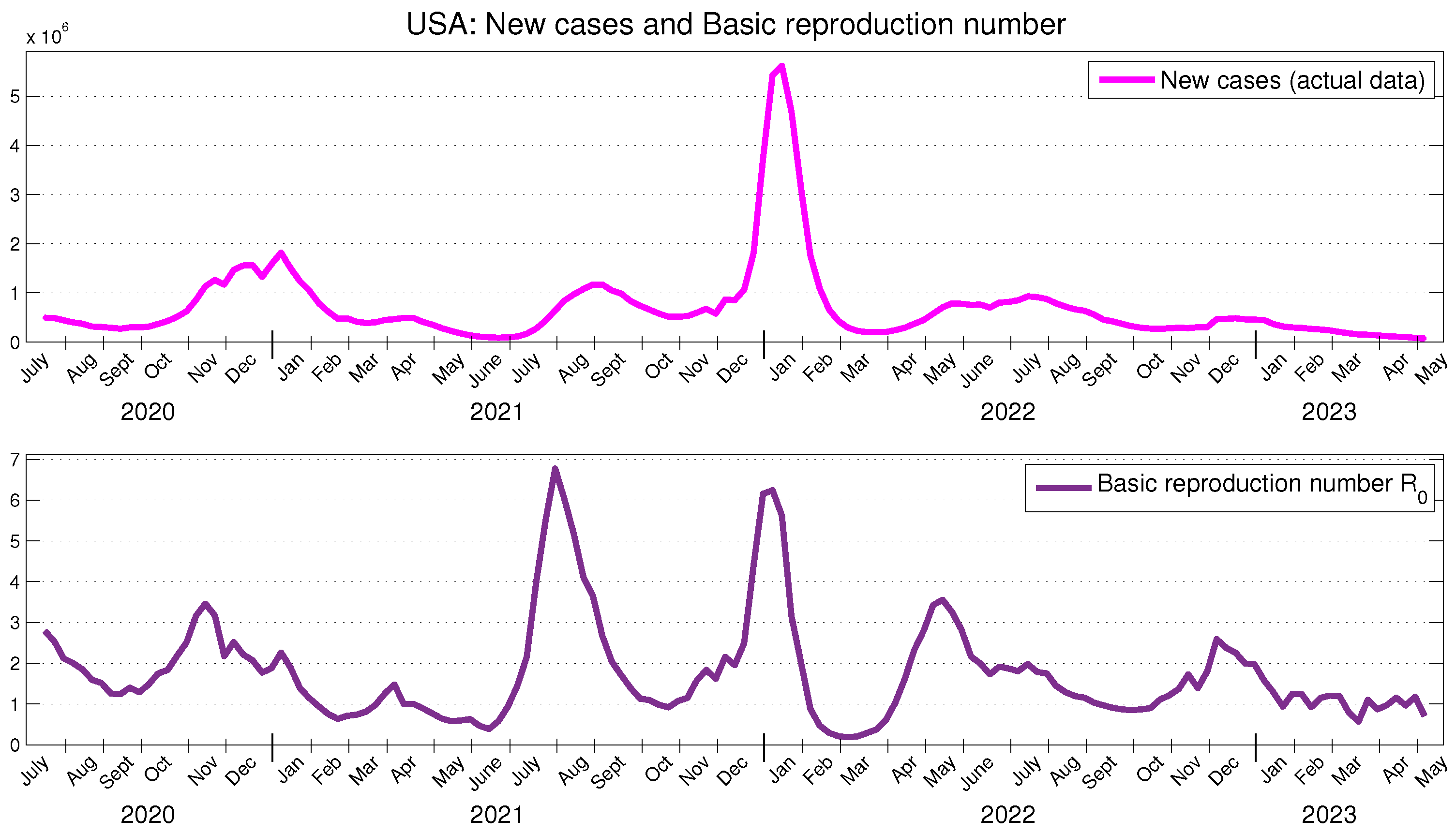
Figure 2 illustrates the officially reported data for new cases in the USA and the obtained results for ${\Re }_0\left(t\right)$. The obtained results for ${\Re }_e\left(t\right)$ are presented in Figure 3. We observe that the changes in the behavior (increase, decrease, local maximum, local minimum) of the basic and effective reproduction numbers occur approximately three or four weeks prior to the similar changes observed in the behavior of new cases.

These findings can be compared with similar studies from other authors. For instance, we observe a strong alignment in both the behavior and values of the time-dependent basic and effective reproduction numbers shown in Figure 2 and Figure 3 and those obtained in [27]. The curve of the evolution of the effective reproduction number over the timeframe between July 2020 and June 2021 given in [40] has similar behavior to that in Figure 3, only with smaller peaks. The estimated daily values of the time-dependent effective reproduction number for the period from August to December 2021, as presented in [41], in our view, have average weekly values that closely align with those shown in Figure 3.

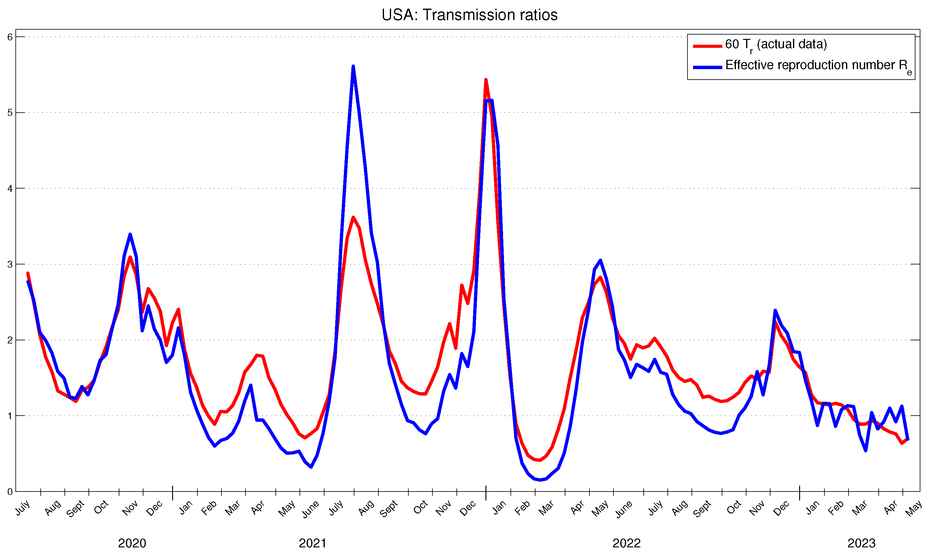
The actual transmission ratio $T_r$, scaled by 60, is presented in Figure 3. As anticipated, it can be observed that the behavior of the $T_r$ closely aligns with the behavior of the effective reproduction number. As an assessment of the realization of the potential of the SARS-CoV-2 in the USA, we highlight that, for the period under consideration, the average value of the actual transmission ratio $T_r$ represents approximately 2.11 % of the average value of the effective reproduction number ${\Re }_e$.

5.2. Application to the COVID-19 Data in Italy

• Epidemic period under consideration: 30 March 2020–11 June 2023 (167 weeks).
• Data Availability: Data regarding active cases, recovered individuals, and deceased individuals is available at [2].The data for Hospitalized patients and patients in ICU can be found at [3]. These data have been utilized for the numerical experiments conducted in this research.
• Parameters and initial data values: The initial value for the population size N₁ = 59,500,579 is available at [5]. The additional necessary initial data has been calculated using the aforementioned sources. The birth and mortality rates per year are accessible at [5]. Furthermore, we calculate the COVID-19 mortality rates per year available and calculate natural mortality rates. We obtain the following daily values of birth and natural mortality rates: $\mathrm{\Lambda }=(2.0249\times {10}^{-5},1.9923\times {10}^{-5},1.9600\times {10}^{-5},1.9277\times {10}^{-5})$ and $\theta =(2.5782\times {10}^{-5},2.6521\times {10}^{-5},2.7504\times {10}^{-5},2.9686\times {10}^{-5})$ for the days of 2020, 2021, 2022 and 2023, respectively.

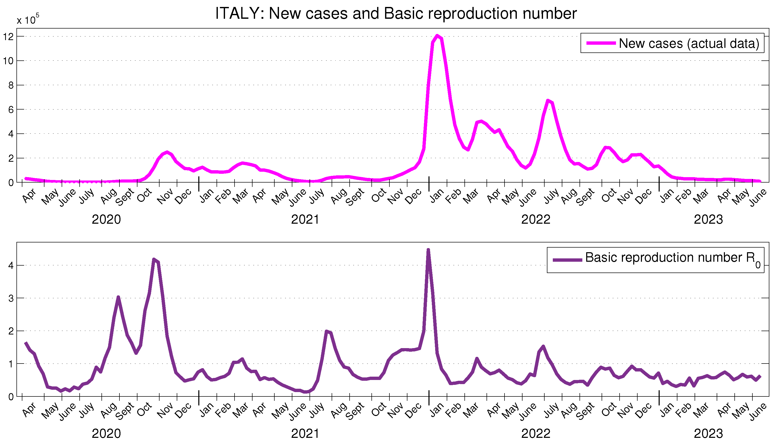
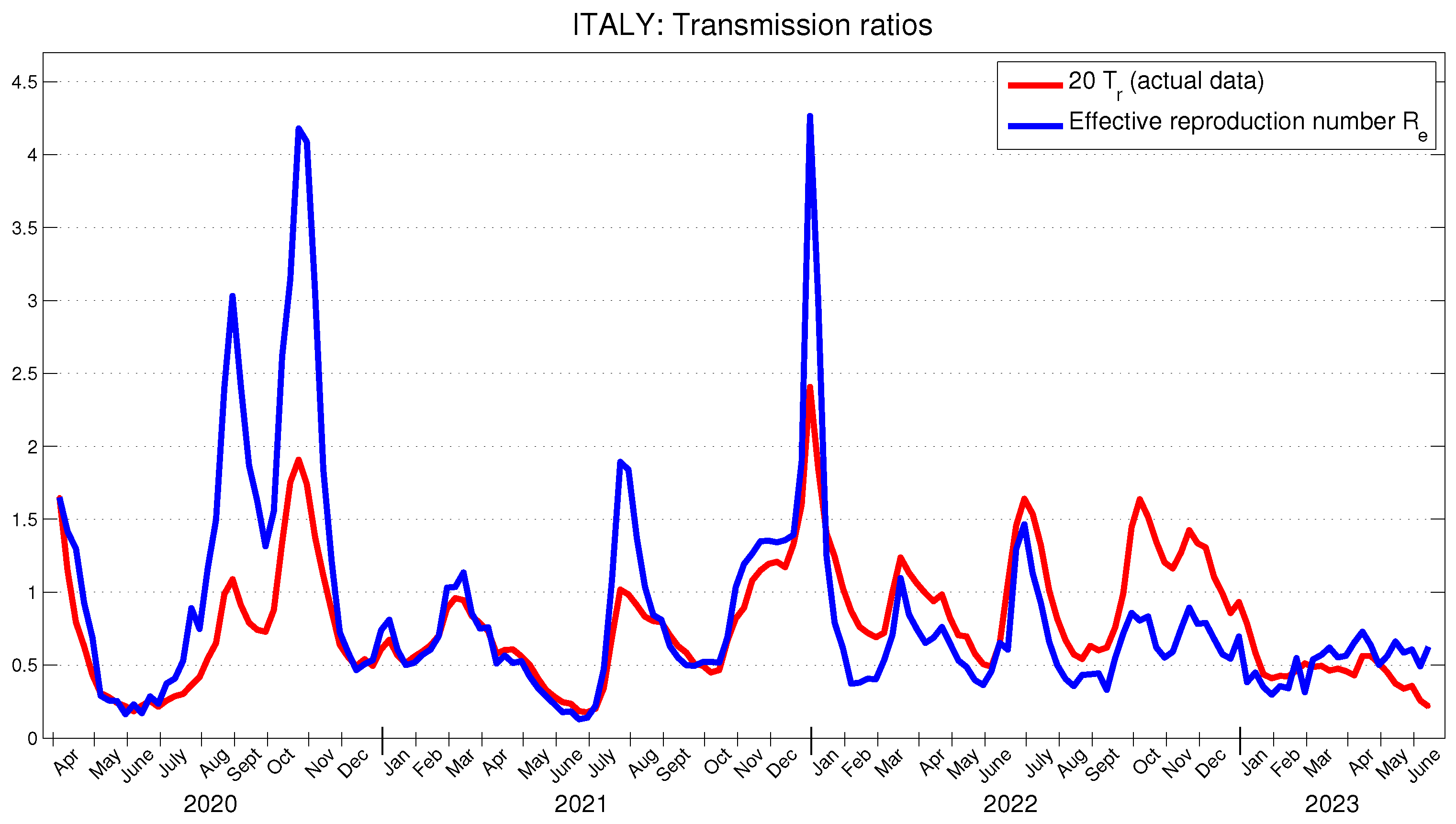
In [42], using reported COVID-19 cases from 1 September 2020 to 27 October 2020, the basic reproduction number ${\Re }_0$ for the second wave in Italy is estimated at 2.83 (95 % CI: 1.5–4.2). The time-dependent basic reproduction number for Italy, shown in Figure 4, during the same period takes values on the interval 1.32–4.18, with a mean value of 2.34. On the other hand, the time behavior of the effective reproduction number in Figure 5 and that in [40] for the period between July 2020 and June 2021 are quite similar, differing only in the magnitude of the two peaks observed in the summer and autumn of 2020.

Figure 5 presents the behavior of the actual transmission ratio $T_r$, scaled by 20. It can be observed that it is similar to the behavior of the effective reproduction number ${\Re }_e$ and, moreover, in Italy, the average value of $T_r$ is approximately 5.38 % of the average value of ${\Re }_e$.

5.3. Application to the COVID-19 Data in Bulgaria

• Epidemic period under consideration: 16 March 2020–12 March 2023 (156 weeks).
• Data Availability: Data regarding active cases, recovered individuals, deceased individuals, and hospitalized patients and patients in ICU are available at [7,8].
• Parameters and initial data values: The initial value for the population size N₁ = 6,951,482 is available at [5]. The additional necessary initial data has been calculated using the aforementioned sources. The birth and mortality rates per year are accessible at [5]. Furthermore, we calculate the COVID-19 mortality rates per year and obtain the following daily values for birth and natural mortality rates: $\mathrm{\Lambda }=(2.4205\times {10}^{-5},4.4041\times {10}^{-5},2.3874\times {10}^{-5},2.3710\times {10}^{-5})$ and $\theta =(3.9501\times {10}^{-5},3.3284\times {10}^{-5},3.9777\times {10}^{-5},4.2797\times {10}^{-5})$ for the days of 2020, 2021, 2022 and 2023, respectively.

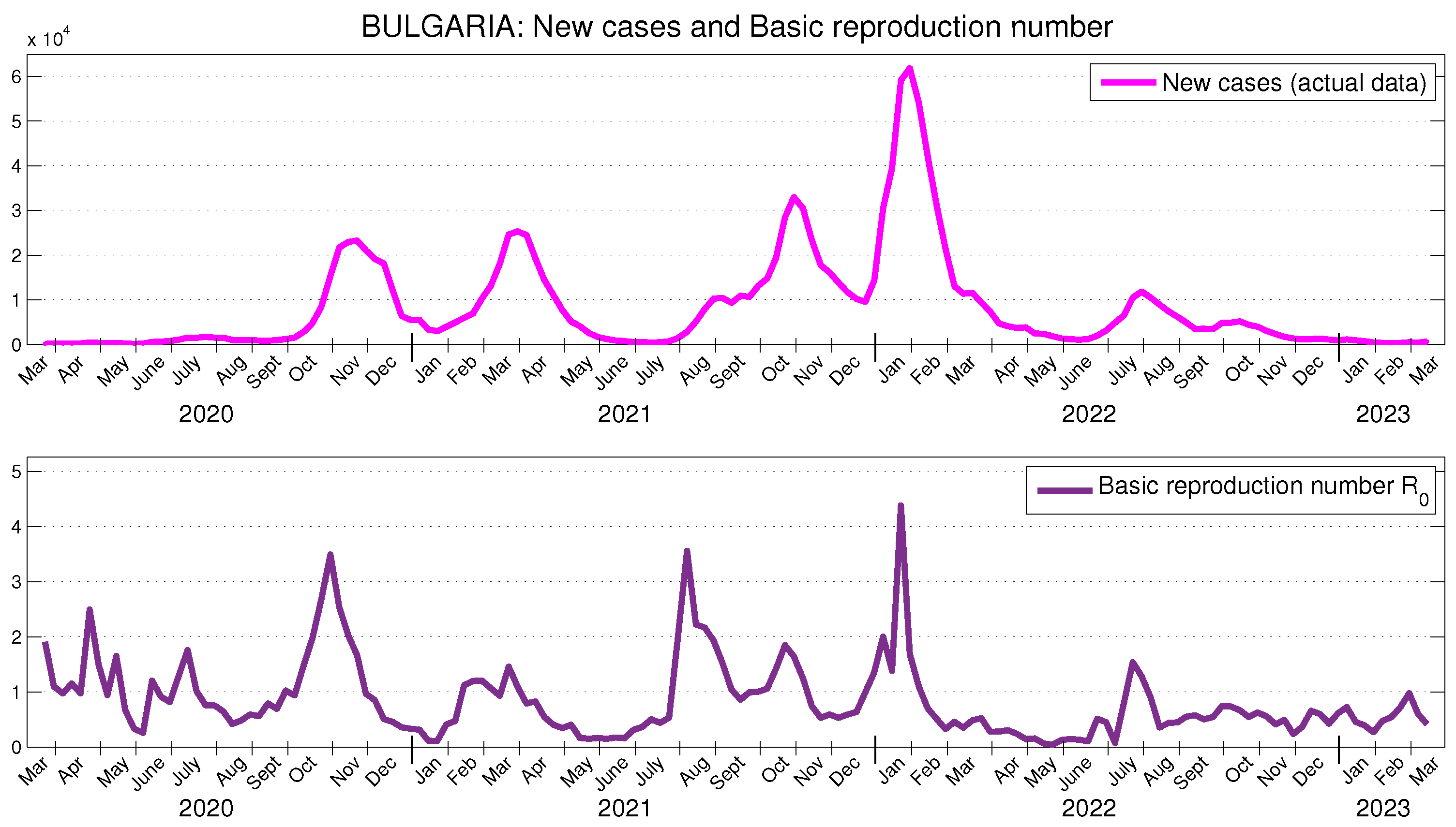
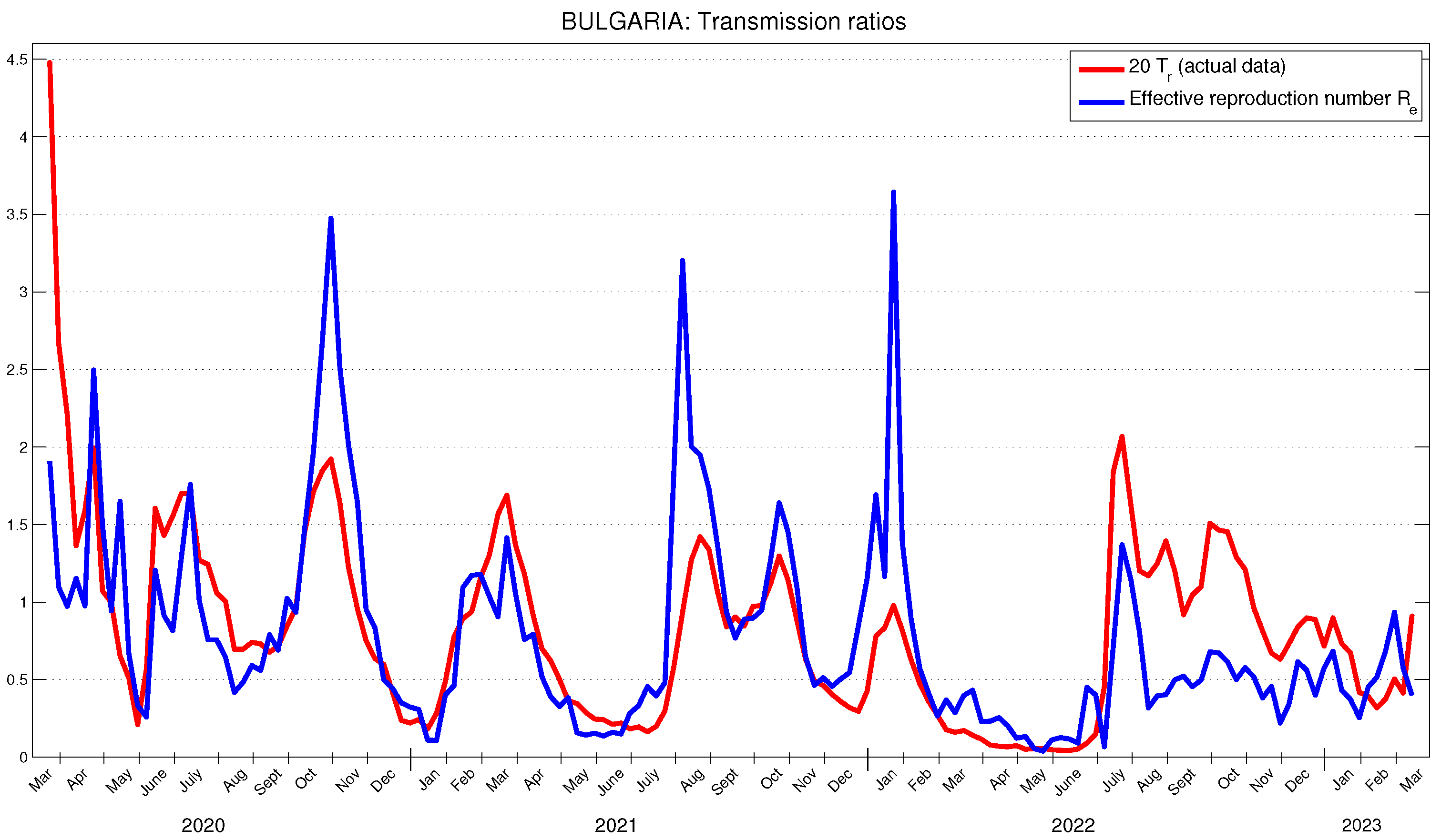
The officially reported data for new cases in Bulgaria, and the obtained results for ${\Re }_0\left(t\right)$ on a weekly basis are presented in Figure 6. The obtained results for the effective reproduction number are presented in Figure 7. Again, it can be observed that changes in the behavior of new cases occur approximately three weeks after the corresponding changes in the basic and effective reproduction numbers. The obtained results for the actual transmission ratio $T_r$ are presented in Figure 7. Once again, they manifest a similar behavior. In Bulgaria, the average value of $T_r$ is approximately 6.14 % of the average value of ${\Re }_e$.

In [30], it is stated that the effective reproductive number at the beginning of the pandemic in Bulgaria has been approximately $1.1$. This fully corresponds to the values of ${\Re }_e$ for the period from the end of May to the middle of April 2020, shown in Figure 7. In [28], using Bulgarian data for the period March 2021–February 2023, a time-dependent effective reproduction number for Bulgaria is calculated. The time behavior of this number, when the authors use a 21-day period, is very close (though slightly higher) to the values shown in Figure 7.

6. Discussion

In this paper, we utilize the SEIRS-VBHC model to study the time evolution of the basic reproduction number $R_0$ and the effective reproduction number ${\Re }_e$ for COVID-19 in three countries: the USA, Italy, and Bulgaria. According to the COVID-19 mortality analysis conducted by Johns Hopkins University [43], these three countries rank among the top 20 in the world for the highest COVID-19 mortality rates. Herein, we aim to discuss the underlying reasons for this phenomenon, drawing on the results of our study, as mortality is a critical indicator for any pandemic, particularly for the one caused by SARS-CoV-2. To achieve this objective, we will utilize both the effective reproduction number ${\Re }_e$ and the actual transmission ratio $T_r$ as discussed in Section 5. Additionally, we will incorporate the vaccination and mortality rates for the countries, as reported by Johns Hopkins University [44]. A summary of the countries based on these indicators is presented in

Table 1. Country Summaries.

Country	${\mathit{\Re }}_{\mathit{e}}$ 1	$100{\mathit{T}}_{\mathit{r}}/{\mathit{\Re }}_{\mathit{e}}$ 1	Vaccination Rate 2	Mortality Rate 3
USA	1.37	2.11	81.81%	341.11
Italy	1.07	5.38	84.16%	311.47
Bulgaria	0.82	6.14	30.31%	550.17

¹ Mean values (calculated with SEIRS-VBHC model) of the corresponding periods, considered in Section 5, ² % of the population receiving at least 1 dose [44], ³ COVID-19 deaths per 100,000 population [43].

.

Again, we emphasize that the basic and effective reproduction numbers serve as quantitative indicators of the virus’ transmission potential, while the transmission ratio $T_r$ reflects the actual rate of spread. We observe that among the three countries under consideration, the USA exhibits the highest ${\Re }_e$ and the lowest ratio of $T_r/{\Re }_e$. This suggests that the measures implemented to curb the virus spread have been particularly effective in the United States. However, the peaks of the actual transmission ratios $T_r$ remain comparable to those observed in the other two countries. This may partly explain the high mortality rate in the USA. Meanwhile, Italy boasts the highest vaccination rate among the three countries. However, its $T_r/{\Re }_e$ ratio remains elevated, indicating that social-distancing measures have been less effective. This could also contribute to its high death rate. In contrast, Bulgaria has the lowest effective reproduction number, yet the virus has maximized its transmission potential there, as demonstrated by the highest $T_r/{\Re }_e$ ratio. The challenges in Bulgaria stem not only from ineffective control measures but also from its vaccination campaign, as it has the lowest vaccination rate in the European Union. Consequently, Bulgaria has the second-highest COVID-19 mortality rate in the world, surpassed only by Peru.

7. Conclusions

This work introduces a novel deterministic SEIRS-type model $SEIRS-VBHC$ that incorporates vaccination and hospitalization. The model accounts for the effectiveness of the vaccines administered and the time required for vaccinated individuals to develop antibodies.

By considering the duration of immune responses in both recovered individuals and those with vaccination-acquired immunity, as well as the number of hospitalized individuals, the model is well-suited for calculating both the basic reproduction number ${\Re }_0$ and effective reproduction number ${\Re }_e$.

We provide a methodology for solving an appropriate discrete inverse problem using actual data to identify the parameters necessary for computing the temporal evolution of ${\Re }_0$ and ${\Re }_e$. Our numerical experiments demonstrate that the time-dependent effective reproduction number can serve as a tool for forecasting the peaks in new active cases, as its peaks tend to occur approximately two weeks before the peaks in the number of new active cases.

Strong mathematical conditions are found that are sufficient for component-wise non-negativity of the numerical solution of the considered discrete variant of the model $SEIRS-VBHC$. However, the conducted numerical experiments show that the algorithm for solving the associated inverse problem also works in simpler real-life situations in the USA, Italy, and Bulgaria, where these conditions may not be met.

Moreover, our study reveals a strong correlation between the temporal behavior of ${\Re }_e$ and the ratio $T_r=New active cases/Nonhospitalized active cases$, which can be calculated using reported data. Finally, we present a methodology for comparing the virus’ transmission potential, as determined by ${\Re }_e$, with its actual transmission rate. Similarity of the behavior of ${\Re }_e$ and $T_r$ for each country USA (Figure 3), Italy (Figure 5), Bulgaria (Figure 7) validates the model SEIRS-VBHC.

In our previous papers [33,34], we studied the simpler SEIRS-VB model and used it to make short-term forecasting of the spread of the virus. There, we made model verification and error estimation of the results in that case. Now, in the more complicated new model SEIRS-VBHC there are included additional population groups and equations for them. Actually, the officially reported COVID-19 data do not contain enough information to find all the parameters in this model. Nevertheless, we show in this paper that it is possible to find some parameters that are sufficient to calculate the basic and effective reproduction numbers. We do this by solving an appropriate inverse problem. If more detailed data were available, it would be possible to find all parameters in the model and to make more accurate forecasting of the virus spread.