Abstract
In the context of the global response to climate change and the promotion of an energy transition, the Internet of Things (IoT), sensor technologies, and big data analytics have been increasingly used in power systems, contributing to the rapid development of distributed energy resources. The integration of a large number of distributed energy resources has led to issues, such as increased volatility and uncertainty in distribution networks, large-scale data, and the complexity and challenges of optimizing security and economic dispatch strategies. To address these problems, this paper proposes a day-ahead scheduling method for distribution networks based on an improved multi-agent proximal policy optimization (MAPPO) reinforcement learning algorithm. This method achieves the coordinated scheduling of multiple types of distributed resources within the distribution network environment, promoting effective interactions between the distributed resources and the grid and coordination among the resources. Firstly, the operational framework and principles of the proposed algorithm are described. To avoid blind trial-and-error and instability in the convergence process during learning, a generalized advantage estimation (GAE) function is introduced to improve the multi-agent proximal policy optimization algorithm, enhancing the stability of policy updates and the speed of convergence during training. Secondly, a day-ahead scheduling model for the power distribution grid containing multiple types of distributed resources is constructed, and based on this model, the environment, actions, states, and reward function are designed. Finally, the effectiveness of the proposed method in solving the day-ahead economic dispatch problem for distribution grids is verified using an improved IEEE 30-bus system example.
Keywords:
distributed resources; day-ahead scheduling; multi-agent reinforcement learning; generalized advantage estimation MSC:
68W99
1. Introduction
In recent years, in the context of the global response to climate change and the promotion of an energy transition, the Internet of Things (IoT), sensor technologies, and big data analytics have been increasingly used in the power system, contributing to the rapid development of distributed energy resources. With the integration of a large number of distributed new energy generation resources into the distribution network [1,2], along with the emergence of new distributed flexible resources, such as industrial and commercial adjustable loads and energy storage [3,4], the distribution network is facing significant challenges from increasing volatility and uncertainty. These changes have complicated the economic dispatch of distribution grids. It is necessary to not only consider the impact of fluctuating real-time electricity prices on the cost of purchasing and selling electricity to the superior power grid, but also the synergistic complementarity and supply–demand balance of various distributed resources within the local grid. Therefore, with the increase in resource categories and volumes in the distribution network, the difficulty of economic scheduling strategies will significantly increase, along with the growing need for co-optimizing internal distributed resources [5,6].
In the early stages of distribution network development, algorithms such as mixed-integer linear programming (MILP) [7], multi-objective particle swarm optimization [8], and the alternating direction method of multipliers (ADMM) [9] were used to address economic dispatch problems [10,11], Which integrates more abundant, more complex, and more distributed resources, the new distribution network makes solving the economic dispatch optimization problem more difficult [12]. In recent years, researchers have conducted studies on the application of reinforcement learning methods in distribution network scheduling strategies [13,14,15,16,17], where reinforcement learning algorithms enhance the system’s decision-making capabilities through continuous interaction between agents and the environment, utilizing feedback and evaluation networks and enabling fast online applications through offline training. The literature [13] proposed a voltage control model and algorithm for distribution networks with renewable energy integration, demonstrating the potential of intelligent algorithms in grid control. The literature [14] studied the optimal control of hybrid energy storage systems based on reinforcement learning, emphasizing its application in AC-DC microgrids and improving resource utilization efficiency. The literature [15] explored the distributed operation of battery energy storage systems using double deep Q-learning, highlighting its advantages in uncertain environments. The literature [16] introduced the deep reinforcement learning Rainbow algorithm to optimize the scheduling strategy of wind power and energy storage equipment under the integrated scheduling mode, which significantly improved the operational efficiency of wind power and energy storage systems; the literature [17] constructed a scheduling model aimed at minimizing losses in the distribution network containing renewable energy sources and electrochemical energy storage, and utilized the proximal policy optimization algorithm (PPO) to solve the Markov decision process, which reduced the impact of model prediction error on the optimization results. The above methods use single-agent reinforcement learning algorithms, ignoring the impact of the overall system decision-making on various types of resources, and the single agent relies on real-time communication with the grid system, requiring continuous iteration and information feedback between the grid to achieve synergy among multiple resource types [17,18,19], which increases the complexity of the algorithmic solutions.
The above problem has driven the development of the multi-agent reinforcement learning (MARL) algorithm. The literature [20] models high-frequency and low-frequency power signals as two agents using a power limiter, and with the goal of maximizing the benefit of the energy storage system, the improved multi-agent twin-delayed deep deterministic policy gradient algorithm (MATD3) is applied to optimize the hybrid energy storage output to smooth wind power output while simultaneously extending the lifespan of the energy energy storage equipment. The literature [21] constructed a distribution network scheduling model based on region division, where each region acts as an agent, using multi-agent proximal policy optimization (MAPPO) for offline training and optimizing the system scheduling strategy online based on the training results. The proposed method improves the online solving capability and reduces the operating cost of the distribution network. The proposed method improves the online solving capability of the system and reduces the operation cost of the system. Therefore, the multi-agent algorithm is more suitable for real-world distribution networks with multiple types of distributed resources, which is conducive to guiding the different types of resource agents to learn cooperative control strategies [22].
In summary, the multi-agent algorithm can effectively guide the distribution network scheduling strategy [23,24]. In the current economic dispatch of distribution networks, there are issues such as complex multi-resource collaborative dispatch models, large fluctuations in algorithm optimization, and slow convergence. To address these issues, this paper introduces the GAE agent function to improve the MAPPO agent algorithm, enhancing the training effectiveness and online decision-making ability of the algorithm.
The main contributions of this paper are as follows:
- An improved MAPPO agent algorithm considering the GAE agent function is proposed to enhance the convergence effect of the algorithm in the training process. The current MAPPO algorithm usually uses the Monte Carlo method to obtain the agent function, which is prone to blind trial-and-error, as well as falling into local optima during the training process in the face of the complex distribution network scheduling strategy solving problem. In this paper, the GAE agent function is introduced to enhance the MAPPO algorithm, improving the convergence speed during the training process and further reducing the time of offline training of the algorithm;
- The designed improved MAPPO algorithm framework can balance the bias and variance in the agent’s reward value in the algorithm in the process of updating the distribution network scheduling strategy by introducing a discount factor, clarifying the direction of strategy updates while improving the algorithm’s convergence speed, reducing fluctuations in the agent’s reward value, and enhancing the stability of strategy updates during training;
- A day-ahead economic dispatch model for distribution networks, incorporating distributed resources such as new energy sources and various controllable units, is designed, and its dispatch model is optimized and solved by improving the MAPPO algorithm. This improves the economic efficiency of the scheduling strategy for distribution networks with multiple distributed resources, as well as the online decision-making efficiency.
The remainder of the paper is organized as follows: Section 2 introduces the principle and framework of the proposed method in this paper. In Section 3, an economic dispatch model for distribution networks containing multiple types of distributed resources is constructed. In Section 4, the transformation method of the proposed model based on the improved MAPPO and the scheduling strategy solving process are described in detail. A comprehensive case study is presented in Section 5 to validate the proposed method in this paper. Finally, Section 6 gives the conclusion of this paper.
2. Principle of Improved MAPPO Algorithm
The MAPPO algorithm is an algorithm based on the centralized training decentralized execution (CTDE) framework and an extension of the PPO method to a multi-agent environment. It assumes that agents of the same type share a value function network and a policy network, meaning each agent has both a value function network and a policy network. Therefore, the MAPPO algorithm is suitable for multi-agent problems in collaborative, competitive, and hybrid environments.
For multi-agent reinforcement learning methods, when the number of agents is small, the value function network is simpler, and the direction of policy updates is easy to specify. However, when the number of agents is large, different agents need to make decisions at the same time, and variability in policy update directions among agents can affect the overall environment’s performance. Therefore, the MAPPO algorithm utilizes the PPO algorithm based on the actor–critic (AC) framework to ensure that the strategies grow steadily in a more optimal direction. In this framework, the critic network (CN) observes the relationship between the environment and reward value, updating the advantage function. The actor network (AN) adjusts the policy based on the advantage function provided by the CN, guiding the system to achieve higher rewards. In the strategy updating method, by controlling the policy gradient (PG) and setting the clip truncation function and then controlling the range of the importance sampling weights, the MAPPO algorithm further restricts the gradient and the magnitude of the strategy updating. This step allows the MAPPO algorithm to maximize the objective function while minimizing the probability of selecting disadvantageous actions, ensuring that strategy updates remain controlled and optimal.
2.1. MAPPO Algorithm Framework
The overall framework of the MAPPO algorithm is shown in Figure 1, in which N is the number of agents in the MAPPO algorithm; T is the execution period of the agents; is the local observation information vector of the ith agent at moment k; is the environment state information vector of the ith agent at moment t; is the action vector outputted by the strategy network of the ith agent at moment t; is the output implied state of the value function network of the ith agent at moment t; is the output implied state of the strategy network at the recurrent neural network (RNN) layer at moment t; is the hidden state of the output of the RNN layer of the value function network at time t; and is the reward for agent i after interacting with the environment at time t. In the training process of the MAPPO algorithm, the strategy network obtains and according to the local observation information of the environment, and stores , , and into the experience pool. The value function network outputs and according to the environmental state information vector and stores , , and into the experience pool. After a period of operation, the complete data link is sampled from the experience pool to update the parameters of its policy network and value function network .
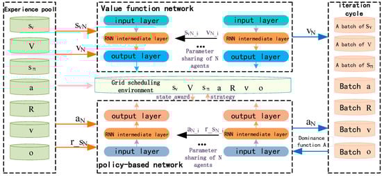
Figure 1.
Framework diagram of MAPPO algorithm.
2.2. Improved Method Based on Generalized Advantage Estimation Function
In the MAPPO algorithm, strategy updates are primarily based on the estimation of the agent’s advantage function. The agent’s advantage function is usually estimated using the Monte Carlo method, as shown in Equation (1).
where is the discount factor with a value range of ; is the reward payoff value of the kth agent at moment t; and is the reward baseline value.
In the process of using the Monte Carlo method for strategy enhancement, the unbiased estimation of the algorithm is achieved, but the variance of the strategy update is still large [25], which affects the learning of the strategy to achieve the action strategy with a higher cumulative reward value, subsequently affecting the convergence effect of the algorithm. Due to the higher number of types and number of distributed resources accessed in the distribution network, the state space and action space of the subject agents are more complex, which has higher requirements for the convergence effect of the algorithm’s strategy update; thus, it is necessary to balance the bias and variance in the agent estimation value to improve the learning efficiency and convergence effect of the algorithm. GAE is an agent estimation function that draws on the idea of λ-return through the introduction of the discount factor. It can balance the bias and variance in the reward value of the agent in the algorithm [26] and improve the speed of the algorithm’s iterative convergence in the training process. The agent estimation function based on the λ-return idea is shown in Equation (2).
where is the GAE agent estimation function value of the first agent; is the introduced discount factor; and is the current iteration step of the algorithm.
Based on this, the optimization objective function of the policy network is shown in Equations (3) and (4).
where B is the batch size of training; is the number of agents in the distribution network model, i.e., the number of distributed resources that can be dispatched in this paper; is the cumulative reward value of the agent in the environment as of time ; is the limiting function, which limits the value of x to [y, z]; is the magnitude of the change in the agent’s action; is the control entropy coefficient; and is the entropy of the strategy, the value function network. The optimization objective function of the strategy is shown in Equation (5).
where is the environment state information of the first agent and is the discount reward.
3. Distribution Network Economic Dispatch Models
In this paper, a dispatch model is constructed with the objective function of minimizing the operating cost of the distribution network, including three types of distributed resources, namely conventional gas turbines, adjustable loads, and energy storage.
3.1. Objective Function
The objective function of this paper is specifically shown in Equation (6). Among them, the distribution grid day-ahead dispatch operation cost mainly includes the system network loss cost, the system cost of purchasing and selling electricity to the higher-level grid, the gas turbine power generation cost, the distributed wind and solar power generation operation cost, the energy storage operation cost, and the adjustable load compensation cost.
where T is the scheduling cycle; indicates the total number of transmission lines in the distribution network; is the network loss cost, where the network loss cost of the distribution network is a uniform value; is the active network loss of the line; is the cost of purchasing and selling electricity from the higher-level grid in time period t; and are the operation and maintenance costs of the grid-connected distributed wind power and photovoltaic stations, which indicate the average operation and maintenance costs of distributed wind power and photovoltaic power production units; and is the operating cost of the ith gas turbine unit in time period t. In this paper, only the cost of electricity consumed by the energy storage system in the charging and discharging process is considered; therefore, the cost of electricity [27] is used to calculate the operating cost of the energy storage system, which is defined as the coefficient of electricity cost of , the cost of compensation for the regulation of the ith adjustable load in time period t. The relationship between the operating cost of the gas turbine unit and the generated active power can be approximated by a quadratic function [28], as shown in Equation (7).
where and are the cost coefficients of the gas turbine unit. The cost of purchasing and selling electricity from the superior grid can be expressed by Equations (8) and (9). The network loss of the distribution grid system is calculated as shown in Equation (10).
where and are the selling and purchasing prices of the superior distribution grid at time t. is the purchasing and selling price of electricity obtained by combining the quadratic relationship between the peak–valley time-sharing price and the net load; denotes the purchasing price of electricity from the superior distribution grid and denotes the selling price of electricity to the superior distribution grid; and denote the voltage amplitude of node i and node j; and denote the voltage phase angle between node i and node j; and and denote the line resistance and reactance between node i and node j, respectively.
Adjustable load compensation adopts a segmented compensation mechanism. This paper sets a regulation compensation coefficient to provide the unit compensation price for different degrees of adjustable loads with different degrees of participation in the regulation, and the unit compensation price consists of the product of the regulation compensation coefficient and the price of electricity purchased and sold by the distribution network to the higher-level power grid [29]. Based on this, this paper sets the load-adjustable range of node i in time period t to be up to 40% and distinguishes the regulation ratio of the adjustable load into shallow and deep regulation areas. When the adjustable load regulation ratio of node is at 0–20%, it is in the shallow regulation area, and the compensation coefficient is a fixed value of 0.4, and when the adjustable load regulation ratio of node is at 20~40%, it is in the deep regulation area, and the compensation coefficient is a quadratic function related to the regulation ratio. The calculation equation is as shown in Equations (11)–(13).
where is the compensation factor of the adjustable load of distribution network node i in time period t and is the regulation ratio of the adjustable load of distribution network node i in time period t, i.e., the ratio of the regulation amount to the load of the node.
3.2. Constraints
3.2.1. Current Constraints
3.2.2. Nodal Voltage Constraints
3.2.3. Interaction Constraints with Higher-Level Grids
3.2.4. Gas Turbine Constraints
The active, reactive, creep, and capacity constraints of the gas turbine are shown in Equations (18)–(20).
where and are the upper and lower limits of the power generation of the ith gas turbine unit; and are the maximum upward and downward creep limits of the ith gas turbine unit; and is the installed capacity of the inverter of the ith gas turbine unit.
3.2.5. Distributed Wind and Photovoltaic Output Constraints
3.2.6. Energy Storage Constraints
The charging and discharging, active and reactive capacity, and number of use constraints of the energy storage system are shown in Equations (23)–(27).
where and are the maximum charging and discharging power of the ith energy storage system; is the capacity of the ith energy storage system at time t; and are the minimum and maximum capacity of the ith energy storage system; and are the charging and discharging efficiencies of the ith energy storage system; is the maximum capacity of the ith storage system connected to the inverter; is the sum of the number of consecutive actions of the storage system up to moment , and the number of times of the charging and discharging conversions is added to one; and is the maximum number of actions of the storage system during the learning cycle.
3.2.7. Adjustable Load Restraint
4. Transformation of Economic Dispatch Model for Distribution Network Based on Improved MAPPO Algorithm
4.1. Design of Action Space
For the distribution grid system environment, the action space includes the action values of all the agents, specifically the power purchase and sale to the higher grid, the gas turbine units, the energy storage units, and the adjustable load action values. The action space is represented in Equation (29); however, since the action range of the agents of reinforcement learning is [−1,1], the outgoing value of the agents in the actual environment is converted to the creep factor, specifically as shown in Equation (30).
In the equation, the action value of the ith agent at time t takes the value interval of ; indicates the climbing limit of the i th agent. When the action value of is positive, the up-climbing limit is selected, and when the action value is negative, the down-climbing limit is selected.
4.2. State Space Design
The state space is the environmental information obtained by the agent through perception, which will guide the agent body to make decisions. In this paper, it is assumed that each agent of the improved MAPPO algorithm is able to perceive the environmental information within the region of nodes from itself, including the scheduling moments of each node in the region and the active power and reactive power of the load. If the current agent belongs to the type of micro gas turbine , in order to avoid the situation of gas turbine climbing and overstepping the limit when the agent makes a decision, the active power output of the gas turbine at the previous moment and the reactive power output of the gas turbine are taken as a part of the state space of the current agent, as shown in Equation (31).
If the current agent belongs to the type of energy storage system , in order to solve the phenomenon of energy storage charging and discharging exceeding the limit that occurs in the decision-making process of the agent, the storage capacity of the previous moment and the number of storage actions up to the previous moment are introduced into the state space, as shown in Equation (32).
If the current agent belongs to the type of adjustable load , in order to limit the amount of adjustable load that occurs in the decision-making process of the agent to overstep the limit, the load-adjustable coefficient and the price of the adjustable load subsidy at time are introduced into the state space, as shown in Equation (33).
4.3. Design of the Reward Function
The reward function is designed to guide the generation of economic and secure scheduling plans for distribution networks containing multiple types of distributed resources. In this paper, the reward function of the distribution grid scheduling plan mainly includes the economic operation cost of the distribution grid , the node voltage overrun penalty , the agent action overrun penalty , the storage agent SOC overrun penalty , the storage agent charging and discharging time overrun penalty , and the distribution grid system purchasing and selling electricity to the superior grid overrun penalty , as shown in Equations (34)–(40). The improved MAPPO algorithm can maximize the reward by continuously updating the value function through feedback and evaluation.
where is the number of nodes in the ith agent sensing region; is the voltage of the jth node in the ith agent sensing region at time t; is the base voltage; and are the voltage penalty coefficients, respectively, and is taken; is the maximum change in the capacity of the initial storage system; is the number of charging and discharging times of the storage system at time t; and is the maximum number of charging and discharging times of the storage system, and this value is taken as four in this paper. See Table A7 in Appendix A for the super reference table of the improved MAPPO algorithm.
4.4. Solution Flow
The improved MAPPO algorithm solves the economic scheduling problem containing multiple types of resources in the distribution network before the day, as shown in Figure 2, which illustrates the optimization process for any single agent. The other resource agents in the distribution network perform the optimization process synchronously and interact with each other following the principle of “centralised training-distributed execution”, with each resource agent following the same optimization process. The observable information of different types of agents is shown in Equations (31)–(33), and the observable range of each agent is shown in Table A8 of Appendix A. The specific solution steps are as follows:
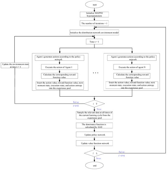
Figure 2.
Flowchart of the solution.
Step 1: initialize the hyperparameters of the improved MAPPO algorithm.
Step 2: initialize the distribution network environment state and set the initial scheduling time.
Step 3: generate actions based on each agent’s policy network, send the actions to the environment for execution, and return the reward and the next observation state for each agent along with their current operational states.
Step 4: insert the action values, reward function values, environment states, execution states, and action entropy for the current moment into the experience pool for that scheduling time.
Step 5: If the scheduling time is less than the optimal set length, increment the scheduling time by one step and return to Step 3. If the scheduling time exceeds the optimal length, sample the data from all moments in the experience pool, compute the overall advantage function using GAE, and update the policy and value function networks using Equations (3) and (5).
Step 6: If the number of iterations is less than the maximum set iterations, increment by one and return to Step 2 for the next learning cycle. If the maximum iterations are reached, end the loop and output the results.
5. Example Analysis
In order to verify the effectiveness of the improved MAPPO algorithm proposed in this paper for the optimal scheduling strategy study of a distribution network containing distributed wind power, gas turbine power, adjustable loads, and energy storage, the improved IEEE 30-bus distribution network is used as an example for a simulation study, with access to five conventional gas turbines, two energy storage systems, and one adjustable load; the system topology is shown in Figure 3.
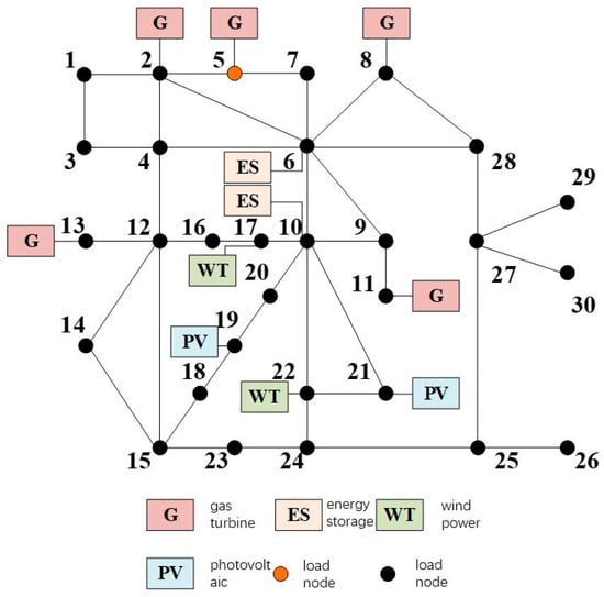
Figure 3.
System topology.
In this paper, the grid-connected node is {1}; conventional gas turbines are connected to nodes {2, 5, 8, 11, 13}; wind turbines are connected to nodes {17, 22}; photovoltaic (PV) units are connected to nodes {19, 21}; energy storage units are connected to nodes {6, 10}; the node of adjustable loads is {5}; and the specific parameters of the distributed resources of the distribution grid are shown in Appendix A (Table A1, Table A2, Table A3, Table A4, Table A5 and Table A6). The distribution grid active network loss cost is RMB 440/MW. In this paper, the scheduling cycle is 24 h, and each hour is a unit scheduling period. The tariffs of electricity purchased and sold from the distribution grid to the higher-level grid are shown in Figure 4.
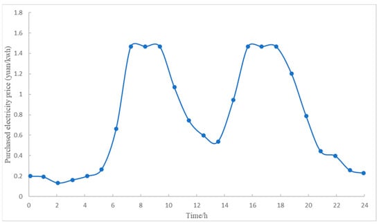
Figure 4.
The distribution network purchases and selling with time-of-use electricity price to the superior power grid.
5.1. Analysis of Improved MAPPO Training Results
In this paper, based on the 24 h load active demand forecast data of a typical day, the active output data of distributed wind and photovoltaic power are predicted in a typical day (see Table A1, Table A2 and Table A3 in Appendix A). The algorithms in this paper were all implemented using Python 3.8.2, with the hardware configuration consisting of a Core (TM) i7-9700K CPU at 3.60 GHz and 32 GB of RAM, the equipment manufacturer name is Intel, the manufacturer’s country is the United States. Both the improved and original MAPPO algorithms were developed based on the PyTorch 1.10 deep learning framework. The critic and actor networks of the base MADDPG algorithm consist of two hidden layers, each containing 64 neurons, with ReLU activation functions applied to all hidden layers. The learning rate was set to 0.0001, and the training steps and maximum batch size were 96 and 20,000, respectively. The improved MAPPO algorithm is trained in 20,000 rounds of iterations based on the distribution network scheduling system, which contains three types of agents, namely gas turbines, adjustable loads, and storage. The results of the training are then analyzed.
Due to the similarity of the rewards and overrun penalties among similar agents, this paper selects a typical agent from each of the gas turbine unit agents, adjustable load agents, and energy storage agents to be analyzed, where the voltage overrun penalty of the agent refers to the sum of the voltage fluctuation penalties that exist at the nodes within the observable range of each agent. The rewards of the gas turbine smart body, the adjustable load smart body, and the energy storage smart body are specifically shown in Figure 5, Figure 6 and Figure 7.
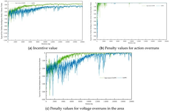
Figure 5.
Typical gas turbine agent reward.
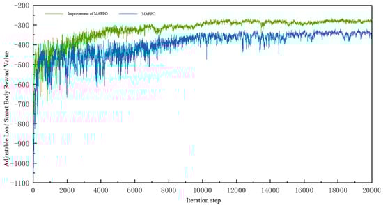
Figure 6.
Typical adjustable load agent reward value.
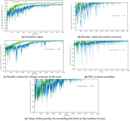
Figure 7.
Energy storage agent reward value.
From the figure, it can be seen that both the MAPPO algorithm and the improved MAPPO algorithm in this paper can effectively train and converge the reward values of all types of agents. Overall, the improved MAPPO algorithm in this paper has a faster convergence speed and better convergence results compared with the MAPPO algorithm. The reward value of the agent converges at about 4000 steps in advance on average, and the convergence stability value is improved by nearly 22.5%. For the action overrun penalty, the node voltage overrun penalty in the observable area, and the overrun penalty set by the energy storage agent, both algorithms are able to converge the penalty value to zero and optimize the operation of each type of agent; however, the improved MAPPO algorithm still has a faster convergence speed. Both algorithms have oscillations in the convergence process, which is caused by the update in the strategy, but the improved MAPPO algorithm has a small amplitude of oscillations and the convergence process is more stable, which indicates that the introduction of GAE in the improved MAPPO algorithm can effectively guide the algorithm strategy to update in a better direction, and the updating amplitude is within the controllable range, which obviously helps the optimization of the objective function.
Figure 8 shows the overall situation of the distribution system under the training of the MAPPO algorithm and the improved MAPPO algorithm. For the gas turbine agent, the overall operating cost of the improved MAPPO algorithm is reduced by nearly 44.5% compared to the MAPPO algorithm. For the adjustable load agent, the MAPPO algorithm has been fluctuating during the iteration process and the fluctuation of the cost in the strategy of each iteration cycle is larger, which depends on the amount of load adjustment in the strategy of each iteration of the MAPPO algorithm. In the training results of the improved MAPPO algorithm, the operating cost of the adjustable load is almost unchanged and at a high level in the pre-iteration period of the algorithm, which is due to the fact that in the pre-optimization period of the algorithm, the cost of the distribution grid system for purchasing electricity from the superior grid may be higher than the compensation for the adjustment of the adjustable load. When the optimization of the algorithm gradually stabilizes, the regulation level and cost of the adjustable load tends to be reduced, and due to the uncertainty of the load demand level at each node and the distributed wind power level, the adjustable load changes its regulation level according to the actual system situation; thus, the cost of the adjustable load fluctuates and tends to be stabilized within a certain range in the later stages of the algorithm.
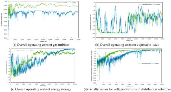
Figure 8.
The overall situation of the distribution network system.
For the overall operating cost of the energy storage smart body, although the MAPPO algorithm eventually converges to a zero value, which is lower than the training results of the improved MAPPO algorithm, the utilization rate of the energy storage of the distribution network system under the training results of the unimproved algorithm is low, and it is not suitable to be used. For the overall voltage overrun penalty of the distribution network, both algorithms can converge to a zero value, but the improved MAPPO algorithm starts to converge nearly 4000 steps in advance, and the convergence process is stable with a low degree of fluctuation.
The above analysis can show that the improved MAPPO algorithm can converge earlier than the MAPPO algorithm, the convergence process is more stable, and the convergence result is better. In addition, the improved MAPPO algorithm is able to use independent and shared structures to perceive and make decisions that are more conducive to the overall goal of the environment, and it can take the global interest as the ultimate optimization goal while taking into account the interests of the agents themselves so that the individual agent can achieve a good performance and at the same time, the economic scheduling goal of the overall system can obtain the optimal result.
5.2. Analysis of the Results of the Improved MAPPO Test
In order to verify the effectiveness of the improved MAPPO algorithm proposed in this paper in solving the day-ahead economic dispatch of distribution grids containing multiple types of distributed resources, the trained MAPPO algorithm is verified based on the 24 h active real demand data of a typical day, as well as the real output data of distributed wind and photovoltaic power units, the collection of which is shown in Figure 9, Figure 10 and Figure 11 as the test data. In the above test data used in this paper, the real-time tariffs of power purchased and sold from the distribution grid to the higher-level grid are consistent with Figure 4.
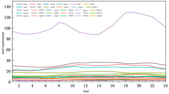
Figure 9.
Real node load demand data.
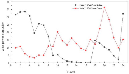
Figure 10.
Comparison of real data and predicted data of wind power output.
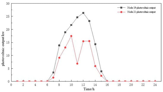
Figure 11.
Comparison of real data and predicted data of photovoltaic output.
After testing, the active output of each gas turbine in the system and the load in the area are obtained, as shown in Figure 12. The regulation of the adjustable load is shown in Figure 13, and the charging and discharging of the energy storage system with the SOC charging state is shown in Figure 14.
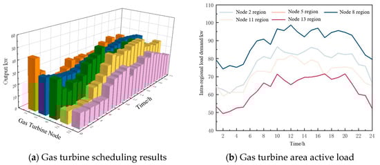
Figure 12.
Actual output of gas turbine agent.
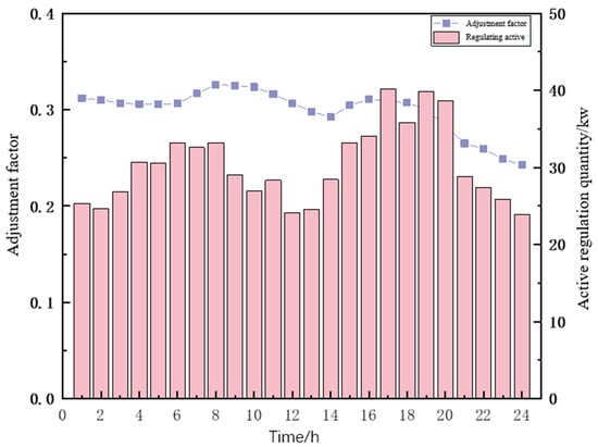
Figure 13.
Adjustable load scheduling results.
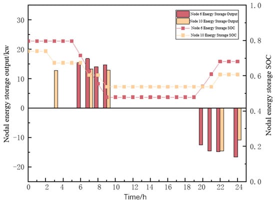
Figure 14.
The actual output of energy storage and SOC situation.
As can be seen in Figure 12, the gas turbines in each region of the system basically follow the changes in the load levels within their regions. According to Figure 12b, it can be seen that the load in the region is in the peak state from 10:00 to 20:00, and according to Figure 12a, the output of all gas turbine units in this time period has a higher output level in this time period. The load in the region is in the valley state from 20:00 to 06:00, and the output of most of the gas turbines decreases in comparison with that in the peak time period. The gas turbines at nodes 2, 5, and 8 have higher outputs at the beginning of the dispatch cycle due to the higher level of observable nodal loads in the region where these three units are located, but the level of distributed wind and PV outputs is lower at that time, so the three units have higher output levels at the beginning of the dispatch cycle.
As can be seen in Figure 13, the amount of adjustable load curtailment at each dispatch moment is kept at 0.25 to 0.35 times of the nodal load to obtain more regulation compensation. Among them, the adjustable load curtailment forms a peak at 06:00–08:00 and 17:00–20:00, where the cost of power purchase from the higher grid by the distribution network and the demand of the nodal load continue to rise. There is a peak at node 5, where the adjustable load reaches a peak at 6:00 a.m. and 20:00 p.m. and falls to a valley at 12:00 p.m.; The adjustable load has a higher compensation price and a greater adjustment potential during the peak period. The regulated loads are compensated at the peak time with higher prices and greater regulation potential, so the reduction in regulated loads peaks at that time; at the trough time, the compensation prices are lower and the regulation potential decreases, so the reduction in regulated loads reaches the trough at that time and continues to decrease with the decrease in load demand after 20:00 p.m.
As can be seen from Figure 14, the operation mode of the energy storage system is low charge and high discharge, charging in the time period when the power purchase tariff from the higher grid is low and discharging in the time period when the power purchase tariff from the higher grid is high, which not only reduces the storage cost of the energy storage system s but also meets the demand of the system during the peak load hours. The energy storage system focuses on discharging operations during the 06:00–09:00 time period, as the distributed wind power is low during this time period, resulting in a high level of net load on the system; as such, the discharging during this period facilitates meeting the load demand during the current time period.
The charging of the energy storage system in the 20:00–24:00 time period helps its SOC state to recover to be similar to the initial state at the end, which satisfies the operation rules of the energy storage system. At the same time, the load is in the valley state in this time period and the gas turbine continues to be in the state of high output operation, and the charging of the energy storage system in this time period can consume the residual output power of the gas turbine. In addition, the number of times the energy storage system is used is two times, which is lower than the maximum number of times the energy storage system is used in this paper. The energy storage system is not in the state of deep charging and deep discharging. The depth of continuous charging is between 10% and 30% and the depth of continuous discharging is between 10% and 40%, which is due to the fact that in the case of where there is a sufficient surplus of power generation from other resources, the shallow charging and shallow discharging of the energy storage system can reduce the maintenance cost of the energy storage system in later stages and increase the whole life cycle of the energy storage system.
From Figure 15, it can be seen that the distributed wind power and photovoltaic units, gas turbines, and energy storage systems, as well as adjustable loads and power purchased from higher-level grids in the system, basically satisfy the total nodal load demand of the system, and the trend in the gas turbine’s output is similar to that of the overall load demand in the whole scheduling cycle. When the power purchase price from the upper-level grid is high in the distribution network, the gas turbine is the main source of system active demand, which effectively reduces the system to higher grid power purchasing at the same time, effectively reducing the operating costs; due to the distributed wind power and photovoltaic power in the evening, power is low or even non-existent, so higher grid power purchasing is the main source of power supply and the cost is lower for the time period. This reduces the overall operating cost of the distribution grid system.
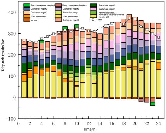
Figure 15.
System active power scheduling results.
In order to ensure the security and reliability of the economic dispatch of the distribution system, it is necessary to consider the voltage constraints at each node of the distribution system as well as the reactive power situation. In Figure 16a, it can be seen that the fluctuations of the voltage at each node within the system are within the range of 0.94 to 1.06, and the fluctuations are relatively small and do not show large fluctuations to pose a threat to the safe and stable operation of the distribution network. From Figure 16b, it can be seen that the fluctuation of the reactive power output of the agent within the system is large, which is due to the changes in the reactive power demand at each node as well as the changes in the real-time operating status of the entire distribution network, meaning that the reactive power output equipment needs to be adjusted quickly and accordingly.
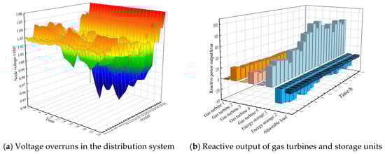
Figure 16.
Other operations of distribution network system.
5.3. Economic Analysis of Algorithm Results
In order to verify the economic benefits of the improved MAPPO algorithm proposed in this paper in solving the optimal scheduling of distribution networks containing multiple types of distributed resources, the system operating costs of the distribution network system before and after the stochastic optimization algorithm and the improvement of the algorithm utilized in this paper for solving the scheduling problem are given in Table 1. Among them, the traditional optimization algorithm adopts the particle swarm optimization (PSO) algorithm, with the algorithm parameters set as follows: particle population size is 50, the maximum number of iterations is 100, the inertia weight is taken to be 0.9, and the learning factor of the individual and population is taken to be two.

Table 1.
System day-ahead scheduling operation cost under various optimization algorithms.
With respect to the cost of different optimization methods, Table 1 shows that the improved MAPPO algorithm used in this paper has the lowest system operating cost in solving the optimal scheduling problem for distribution networks containing multiple types of distributed resources, which is better than those obtained by other algorithms. Compared to the stochastic optimization PSO algorithm, its distribution network operating cost is reduced by 18.1%; compared to the MAPPO algorithm, its distribution network operating cost is reduced by 6.7%.
For the decision times of different optimization methods, the improved MAPPO algorithm in this paper takes only 11.13 s to make an online decision after nearly 11 h of offline training, which is a 21.2% improvement in offline training time and an 18.5% improvement in online decision time compared to the MAPPO algorithm. Compared with the PSO stochastic optimization algorithm, the online decision time is greatly improved, and the total offline training and online decision time of the method used in this paper is improved by 45.7% compared with the PSO stochastic optimization algorithm online decision time.
The results, on the one hand, show that the improved MAPPO algorithm can effectively make better decisions and reduce the cost of distribution network scheduling operations by sensing environmental information through independent and shared decision networks. On the other hand, it shows that the improved MAPPO algorithm effectively improves the solution efficiency of the distribution network active dispatch problem with multiple types of distributed resources.
6. Conclusions
In this paper, to address the problems of increasing volatility and uncertainty in the distribution network due to massive distributed energy access, a huge data scale, and complex and difficult-to-optimize-and-solve security and economic scheduling strategies, a day-ahead economic scheduling model of the distribution network with gas turbines, energy storage systems, and adjustable loads is established, and its optimization objective is to minimize the operating cost of the gas turbine unit, the operating cost of the energy storage system, the compensation cost of the adjustable loads, and the cost of purchasing and selling electricity to the higher grid. The MAPPO algorithm is used to solve the optimization. This method reduces day-ahead scheduling costs and improves the efficiency of the system’s online solution. The following conclusions are obtained through the simulation analysis:
- Compared to traditional optimization algorithms, the MAPPO algorithm significantly reduces decision-making time. The improved MAPPO algorithm is 18.5% faster than the unimproved version, enhancing its solving efficiency.
- The improved MAPPO algorithm has fewer fluctuations in reward values during convergence, and the convergence process is more stable compared to the unimproved MAPPO algorithm, which verifies that GAE further improves the algorithm learning performance.
- The improved MAPPO algorithm achieves the lowest cost in solving the economic dispatch problem for distribution networks with multiple resource types, reducing operational costs by up to 18.1% compared to other algorithms, thus improving the economic performance of the network.
- Future research could further explore the application of the improved MAPPO algorithm in real-time dispatch problems, integrating emerging technologies such as edge computing and artificial intelligence to achieve more efficient energy management. Additionally, research could examine the scalability of the algorithm, particularly in optimizing performance when handling larger more complex distributed networks. Another potential direction includes investigating the coordinated optimization between different types of resources to enhance overall system scheduling and improve the ability to handle unexpected situations.
Author Contributions
Conceptualization, W.T.; Methodology, J.Z., Q.A. and W.T.; Validation, J.Z., Q.A. and W.T.; Investigation, W.W.; Writing—original draft, J.Z.; Writing—review & editing, Q.A. and W.W.; Visualization, W.W. All authors have read and agreed to the published version of the manuscript.
Funding
This research was funded by the National Key R&D Program of China (No. 2021YFB2401203).
Data Availability Statement
The data presented in this study are available on request from the corresponding author due to legal and privacy reasons.
Conflicts of Interest
Authors Juan Zuo and Wenbo Wang were employed by State Grid Shanghai Energy Interconnection Research Institute Co., Ltd. The remaining authors declare that the research was conducted in the absence of any commercial or financial relationships that could be construed as a potential conflict of interest.
Appendix A
Table A1.
Grid node related parameters.
Table A1.
Grid node related parameters.
| Numbering | Grid Node | Maximum Sale of Electricity | Maximum Purchase of Electricity |
|---|---|---|---|
| 1 | 1 | 50 | 50 |
Table A2.
Conventional gas turbine parameters.
Table A2.
Conventional gas turbine parameters.
| Numbering | Access Node | Capacity (kW) | Minimum Starting Capacity (kW) | Maximum Climbing Rate | Minimum Climbing Rate | Cost Coefficient | |
|---|---|---|---|---|---|---|---|
| agas | cgas | ||||||
| 1 | 2 | 80 | 8 | 0.16 | −0.16 | 1.1 | 0.4 |
| 2 | 5 | 80 | 8 | 0.16 | −0.16 | 1.1 | 0.4 |
| 3 | 8 | 60 | 6 | 0.16 | −0.16 | 1.1 | 0.4 |
| 4 | 11 | 60 | 6 | 0.16 | −0.16 | 1.1 | 0.4 |
| 5 | 13 | 60 | 6 | 0.16 | −0.16 | 1.1 | 0.4 |
Table A3.
Distributed wind turbine parameters.
Table A3.
Distributed wind turbine parameters.
| Numbering | Access Node | Capacity (kW) |
|---|---|---|
| 1 | 17 | 60 |
| 2 | 22 | 60 |
Table A4.
Distributed photovoltaic unit parameters.
Table A4.
Distributed photovoltaic unit parameters.
| Numbering | Access Node | Capacity (kW) |
|---|---|---|
| 1 | 19 | 40 |
| 2 | 21 | 40 |
Table A5.
Energy storage unit parameters.
Table A5.
Energy storage unit parameters.
| Numbering | Access Node | SOCmin | SOCmax | ηd | ||||
|---|---|---|---|---|---|---|---|---|
| 1 | 6 | 200 | 40 | 40 | 0.2 | 0.95 | 0.96 | 0.2 |
| 2 | 10 | 200 | 40 | 40 | 0.2 | 0.95 | 0.96 | 0.2 |
Table A6.
Adjustable load parameters.
Table A6.
Adjustable load parameters.
| Numbering | Access Node | Maximum Adjustable Rate | Maximum Climbing Rate | Minimum Climbing Rate | Call Cost |
|---|---|---|---|---|---|
| 1 | 5 | 0.4 | 0.2 | −0.2 | −style (17) |
Table A7.
MAPPO hyperparameters.
Table A7.
MAPPO hyperparameters.
| Parameter | MAPO | Parameter | MAPO | Parameter | MAPO | Parameter | MAPO | Parameter | MAPO |
|---|---|---|---|---|---|---|---|---|---|
| 8 | 20,000 | 0.0001 | 24 | 64 | |||||
| 0.99 | 5 | 0.0001 | 0.2 | 0.95 | |||||
| 0.95 | 64 | 0.1 | 10 | 10 | |||||
| 100 | 10 | 0.1 |
Table A8.
Agent observation area.
Table A8.
Agent observation area.
| Agent | Observable Region |
|---|---|
| Gas1 | {3,4,6,7,9,10,12,14,15,16,28} |
| Gas2 | {1,2,4,6,7} |
| Gas3 | {3,4,6,7,9,10,17,20,21,22,25,27,29,30} |
| Gas4 | {4,7,9,10,17,20,21,22,28} |
| Gas5 | {3,4,6,12,14,15,16,17,18,23} |
| DL | {1,2,4,6,7} |
| Ess1 | {3,4,9,15,17,18,20,21,22,27,28} |
| Ess2 | {7,9,16,19,20,21,22,28} |
References
- Wang, Z.; Ma, S.; Li, G.; Bian, J. Day-ahead-intraday two-stage rolling optimal scheduling of power grid considering the access of composite energy storage plant. J. Sol. Energy 2022, 43, 400–408. [Google Scholar]
- Huang, J.; Zhang, H.; Tian, D.; Zhang, Z.; Yu, C.; Hancke, G.P. Multi-agent deep reinforcement learning with enhanced collaboration for distribution network voltage control. J. Eng. Appl. Artif. Intell. 2024, 134, 108677. [Google Scholar] [CrossRef]
- Liu, F.; Lin, C.; Chen, C.; Liu, R.; Li, G.; Bie, Z. A post-disaster time-sequence load recovery method for distribution networks considering the dynamic uncertainty of distributed new energy sources. J. Power Autom. Equip. 2022, 42, 159–167. [Google Scholar]
- Li, H.; Ren, Z.; Fan, M.; Li, W.; Xu, Y.; Jiang, Y.; Xia, W. A review of scenario analysis methods in planning and operation of modern power systems: Methodologies, applications, and A review of scenario analysis methods in planning and operation of modern power systems: Methodologies, applications, and challenges. J. Electr. Power Syst. Res. 2022, 205, 107722. [Google Scholar] [CrossRef]
- Qi, N.; Cheng, L.; Tian, L.; Guo, J.; Huang, R.; Wang, C. Review and outlook of distribution network planning research considering flexible load access. J. Power Syst. Autom. 2020, 44, 193–207. [Google Scholar]
- Cheng, L.; Wan, Y.; Qi, N.; Tian, L. Review and outlook on the operational reliability of distribution systems with multiple distributed resources. J. Power Syst. Autom. 2021, 45, 191–207. [Google Scholar]
- Liu, H.; Xu, Z.; Ge, S.; Yang, W.; Liu, M.; Zhu, G. Coordinated active-reactive operation and voltage control of active distribution networks considering energy storage regulation. J. Power Syst. Autom. 2019, 43, 51–58. [Google Scholar]
- Wang, S.; Li, Q.; Zhao, Q.; Lin, Z.; Wang, K. Improved particle swarm algorithm for multi-objective optimisation of AC/DC distribution network voltage taking into account source-load stochasticity. J. Power Syst. Autom. 2021, 33, 10–17. [Google Scholar]
- Jin, G.; Pan, D.; Chen, Q.; Shi, C.; Li, G. An energy optimisation method for multi-voltage level DC distribution networks considering adaptive real-time scheduling. J. Grid Technol. 2021, 45, 3906–3917. [Google Scholar]
- Mehrjerdi, H.; Hemmati, R. Modelling and optimal scheduling of battery energy storage systems in electric power distribution networks. J. Clean. Prod. 2019, 234, 810–821. [Google Scholar] [CrossRef]
- Li, J.; Ma, D.; Zhu, X.; Li, C.; Hou, T. Hierarchical optimal economic dispatch of active distribution networks based on ADMM algorithm. J. Electr. Power Constr. 2022, 43, 76–86. [Google Scholar]
- Hu, W.-H.; Cao, D.; Huang, Q.; Zhang, B.; Li, S.; Chen, Z. Application of deep reinforcement learning in optimal operation of distribution networks. J. Power Syst. Autom. 2023, 14, 174–191. [Google Scholar]
- Liao, Q.; Lu, L.; Liu, Y.; Zhang, Y.; Xiong, J. Voltage control model and algorithm for renewable energy-containing distribution networks considering reconfiguration. J. Power Syst. Autom. 2017, 41, 32–39. [Google Scholar]
- Duan, J.; Yi, Z.; Shi, D.; Lin, C.; Lu, X.; Wang, Z. Reinforcement-learning-based optimal control of hybrid energy storage systems in hybrid AC-DC microgrids. J. IEEE Trans. Ind. Inform. 2019, 15, 5355–5364. [Google Scholar] [CrossRef]
- Bui, V.H.; Hussain, A.; Kim, H.M. Double deep Q-learning-based distributed operation of battery energy storage system considering uncertainties. J. IEEE Trans. Smart Grid 2019, 11, 457–469. [Google Scholar] [CrossRef]
- Yu, I.; Yang, J.; Yang, M.; Gao, Y. Integrated scheduling of wind farm energy storage system prediction and decision making based on deep reinforcement learning. J. Power Syst. Autom. 2021, 45, 132–140. [Google Scholar]
- Yang, Z.; Ren, Z.; Sun, Z.; Liu, M.; Jiang, J.; Yin, Y. A security-constrained economic dispatch method for new energy power system based on proximal strategy optimisation algorithm. J. Grid Technol. 2023, 47, 988–998. [Google Scholar]
- Yang, B.; Chen, Y.; Yao, W.; Shi, T.; Shu, H. A review of power system stability assessment and decision-making based on new generation artificial intelligence technology. J. Power Syst. Autom. 2022, 46, 200–223. [Google Scholar]
- Wu, T.; Wang, J.; Lu, X.; Du, Y. AC/DC hybrid distribution network reconfiguration with microgrid formation using multi-agent soft actor-critic. J. Appl. Energy 2022, 307, 118189. [Google Scholar] [CrossRef]
- Wang, X.; Zhou, J.; Qin, B.; Guo, L. Coordinated control of wind turbine and hybrid energy storage system based on multi-agent deep reinforcement learning for wind power smoothing. J. Energy Storage 2023, 57, 106297. [Google Scholar] [CrossRef]
- Zhang, J.; Pu, T.; Li, Y.; Wang, Y.; Zhou, X. Optimal scheduling strategy for distributed power supply based on multi-intelligence deep reinforcement learning. J. Power Grid Technol. 2022, 46, 3496–3504. [Google Scholar]
- Caicedo, A.M.D.; Mejia, É.F.; Luna, E.G. Revolutionizing protection dynamics in microgrids: Local validation environment and a novel global management control through multi-agent systems. J. Comput. Electr. Eng. 2024, 120, 109748. [Google Scholar] [CrossRef]
- Dvir, E.; Shifrin, M.; Gurewitz, O. Cooperative Multi-Agent Reinforcement Learning for Data Gathering in Energy-Harvesting Wireless Sensor Networks. Mathematics 2024, 12, 2102. [Google Scholar] [CrossRef]
- Wang, G.; Sun, Y.; Li, J.; Jiang, Y.; Li, C.; Yu, H.; Wang, H.; Li, S. Dynamic Economic Scheduling with Self-Adaptive Uncertainty in Distribution Network Based on Deep Reinforcement Learning. J. Energy Eng. 2024, 121, 1671–1695. [Google Scholar] [CrossRef]
- Chen, L. Research on Value Functions in Deep Reinforcement Learning. Ph.D. Thesis, University of Mining and Technology, Xuzhou, China, 2021. [Google Scholar]
- Shen, Y. Research on Proximal Policy Optimisation Algorithms for Reinforcement Learning Problems. Ph.D. Thesis, Suzhou University, Suzhou, China, 2021. [Google Scholar]
- He, Y.; Chen, Y.; Liu, Y.; Liu, H.; Liu, D.; Sun, C. Analysis of kWh cost and mileage cost of energy storage. New Technol. J. Electr. Power 2019, 38, 1–10. [Google Scholar]
- Pan, H.; Liang, Z.; Xue, Q.; Zheng, F.; Xiao, Y. Economic dispatch of a virtual power plant with wind-photovoltaic-gas-storage based on time-of-use tariff. J. Sol. Energy 2020, 41, 115–122. [Google Scholar]
- Wang, K.; Zhang, J.; Qiu, X.; Wang, J.; Wang, C. Accurate current sharing with SOC balancing in DC microgrid. J. Electr. Power Syst. Res. 2024, 232, 110386. [Google Scholar] [CrossRef]
Disclaimer/Publisher’s Note: The statements, opinions and data contained in all publications are solely those of the individual author(s) and contributor(s) and not of MDPI and/or the editor(s). MDPI and/or the editor(s) disclaim responsibility for any injury to people or property resulting from any ideas, methods, instructions or products referred to in the content. |
© 2024 by the authors. Licensee MDPI, Basel, Switzerland. This article is an open access article distributed under the terms and conditions of the Creative Commons Attribution (CC BY) license (https://creativecommons.org/licenses/by/4.0/).