
Standard Deformations of Nonlinear Elastic Structural Elements with Power-Law Constitutive Model


Abstract
1. Introduction
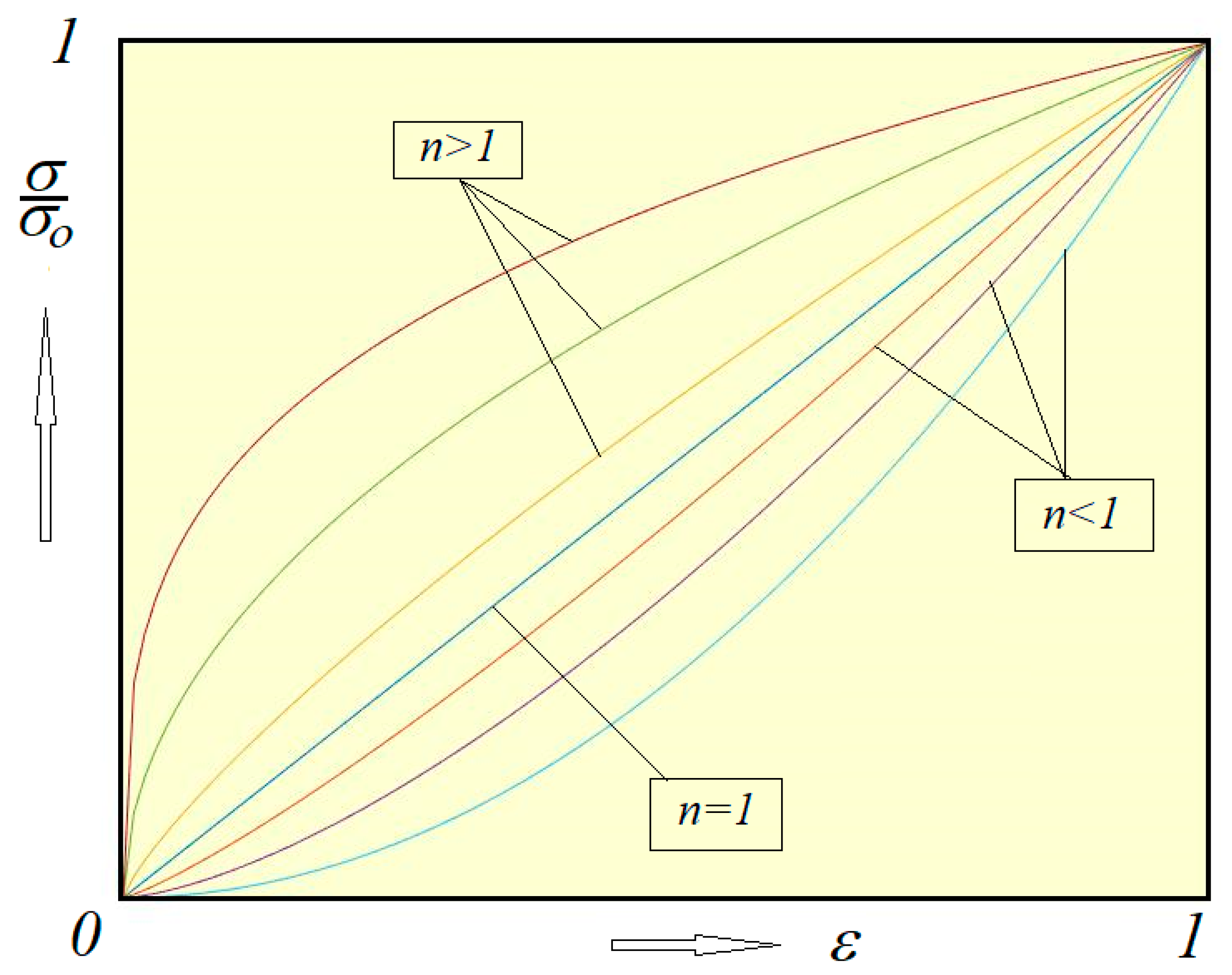
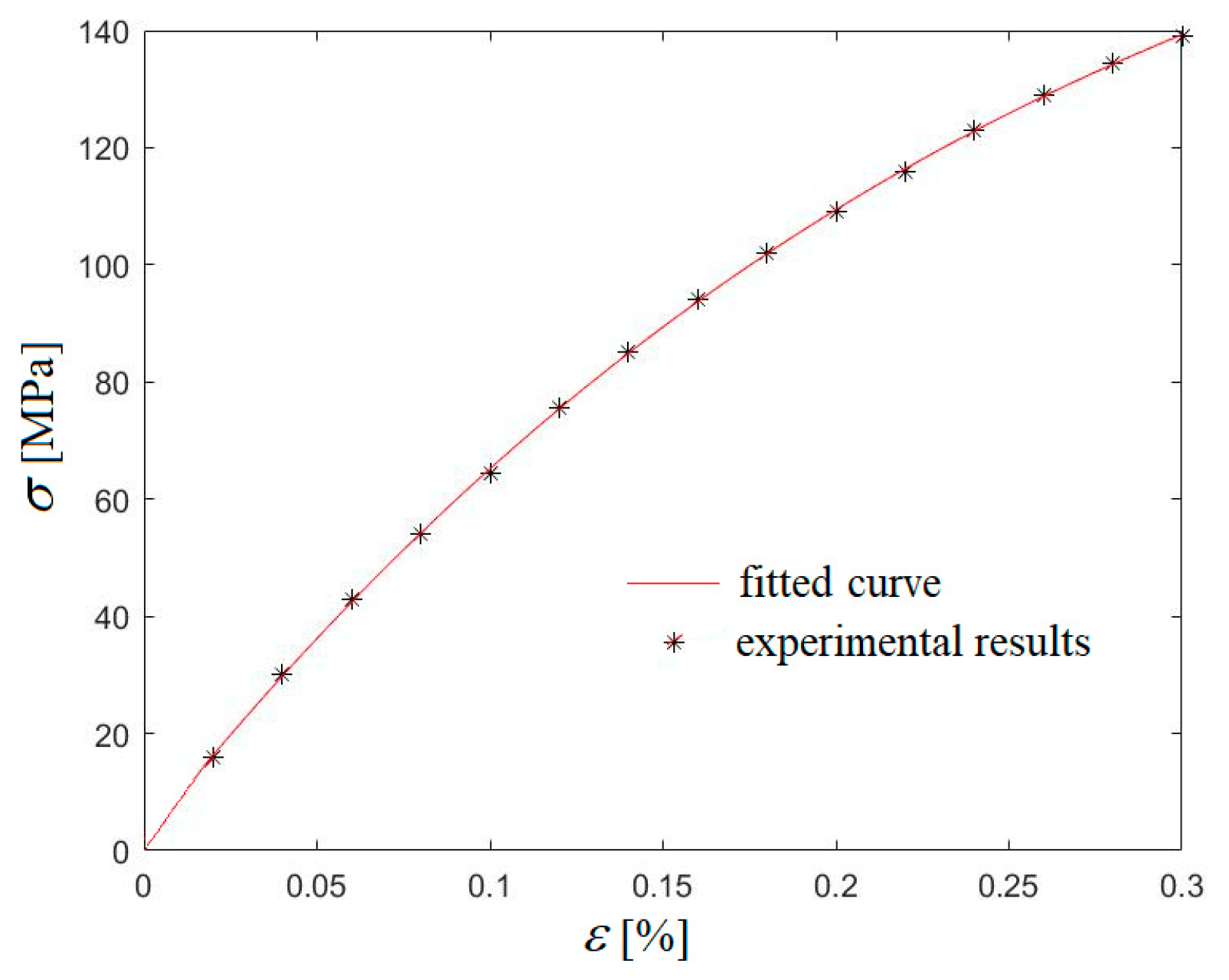
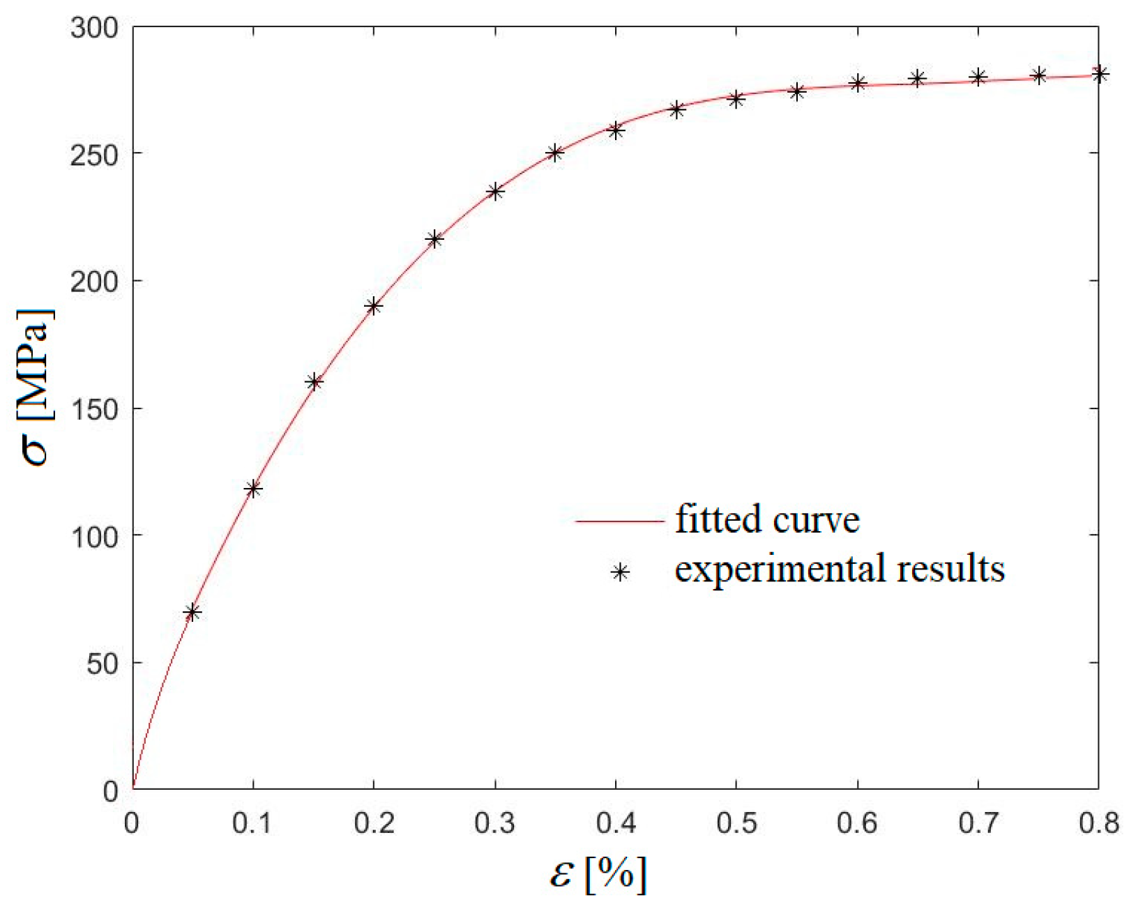
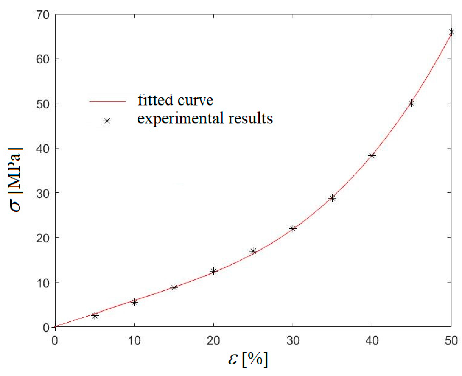
2. Models and Methods: Power-Law Strain–Stress Diagram
3. Results: Basic Loading Cases
3.1. Tension: Compression
- (a)
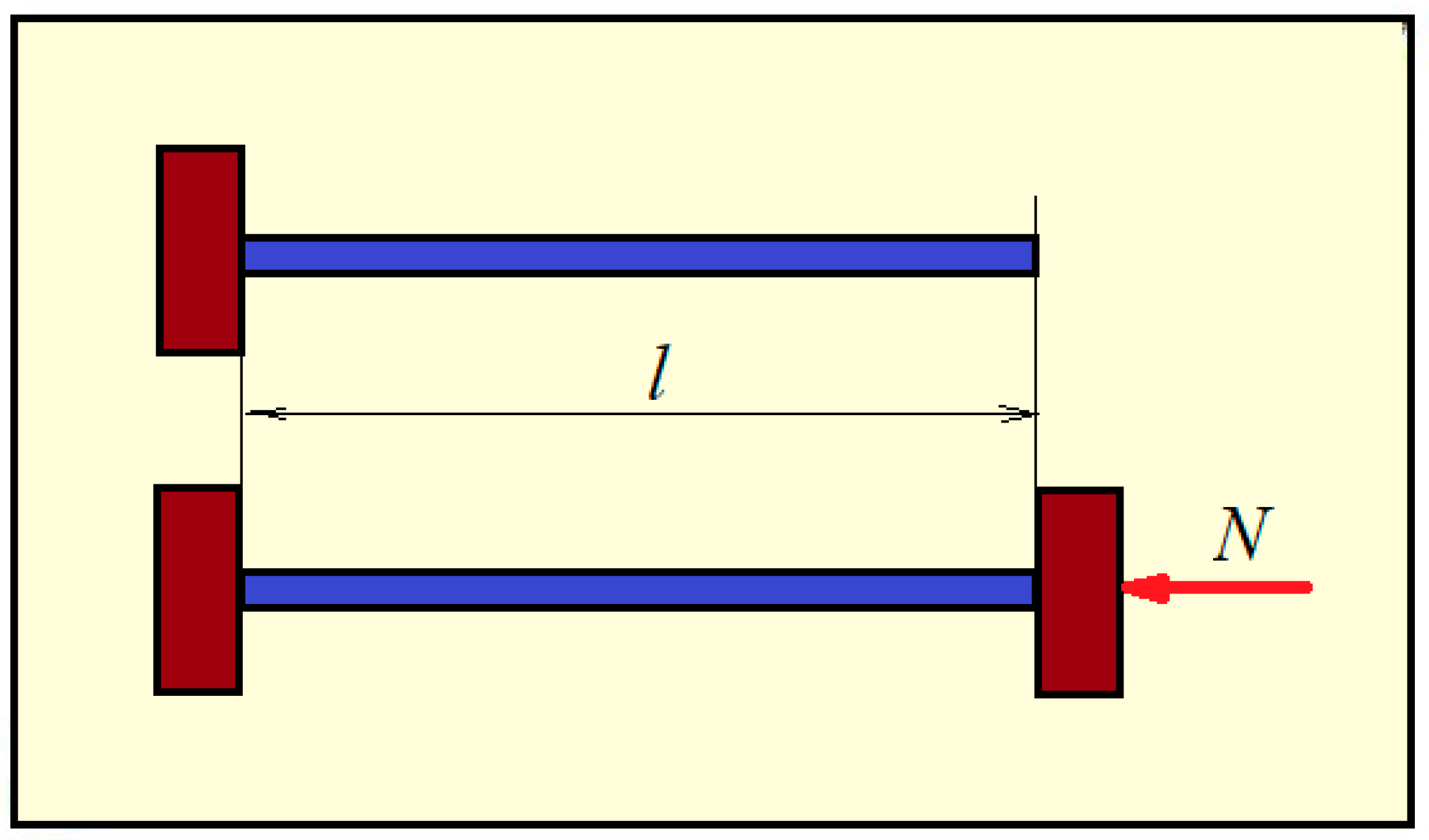
- Assumptions related to linear material resistance are kept, including Bernoulli’s hypothesis. Based on this hypothesis, for one arbitrary section at every point of the section. Therefore, for the points of this section, the stress values are the same:If the normal stress in the section is denoted by N, it can be calculated based on the equilibrium of the stresses acting on the section:This results in(as in linear elasticity). If a bar has the length l and the constant section A, the lengthening/shortening of the bar can be calculated as follows:
- (b)
- In what follows, the case of a bar with an inhomogeneous section is considered. We take the case of a bar made of three different materials marked 1, 2, and 3 (Figure 5). By taking a section and denoting it with , , and , the normal forces on the three materials from the balance equation are deduced:The three materials working together in tension/compression have the same deformation and result:orSubstituting the values of and extracted from relation (11) in Equation (10), we obtainBased on Equation (12), can be taken out using a numerical method for solving the equation. Then, it is simple to obtain and using Equation (11).
- (c)
- If a uniformly heated bar is prevented from expanding, it will be subjected to compression (Figure 6). The compression force (N) is calculated as follows. Noting the temperature difference with , linear expansion is expressed aswhere is the coefficient of linear expansion. Using Equation (8), we obtainwherefrom we can obtainThe normal stress is
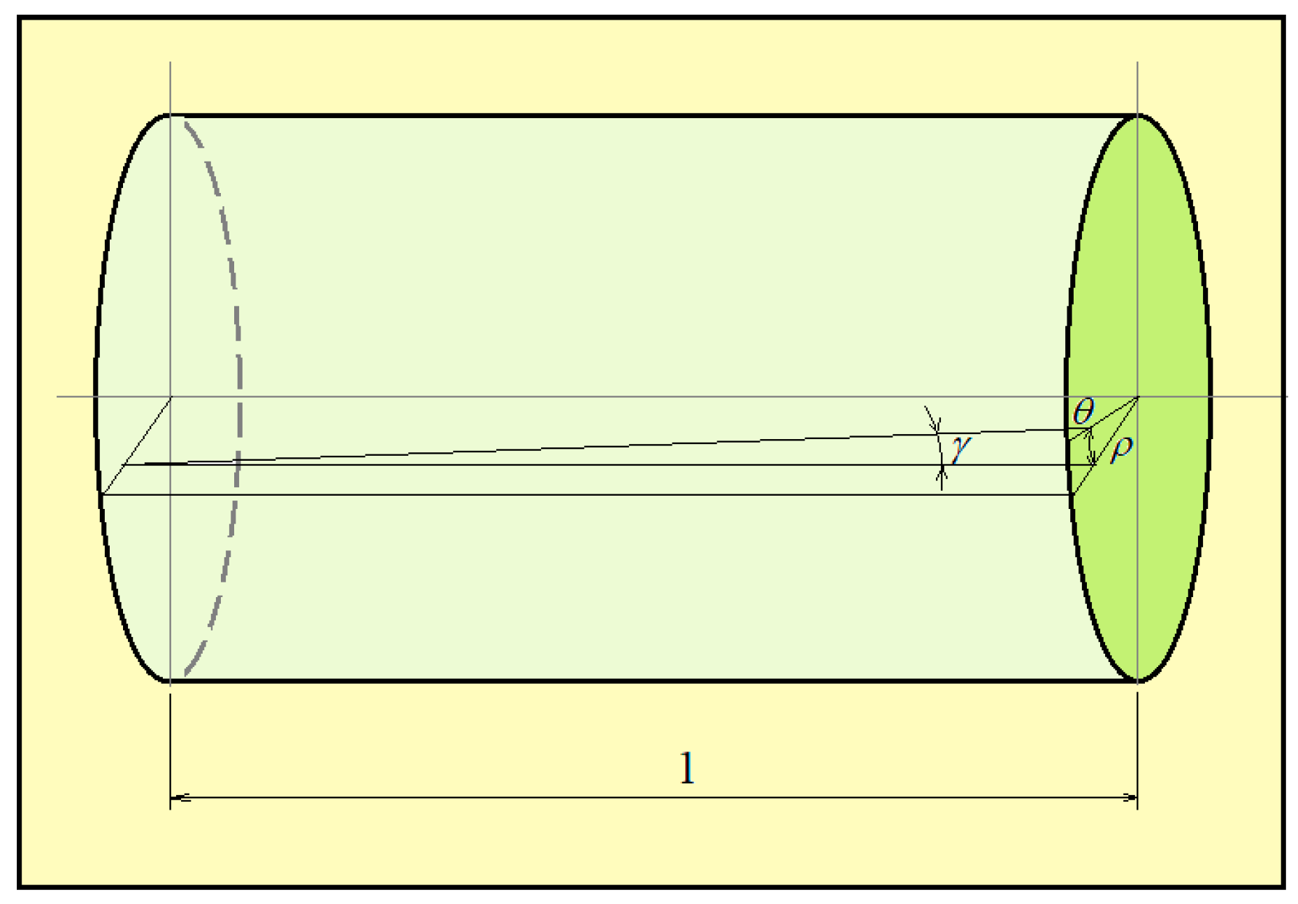
3.2. Torsion of Bars with Circular Sections
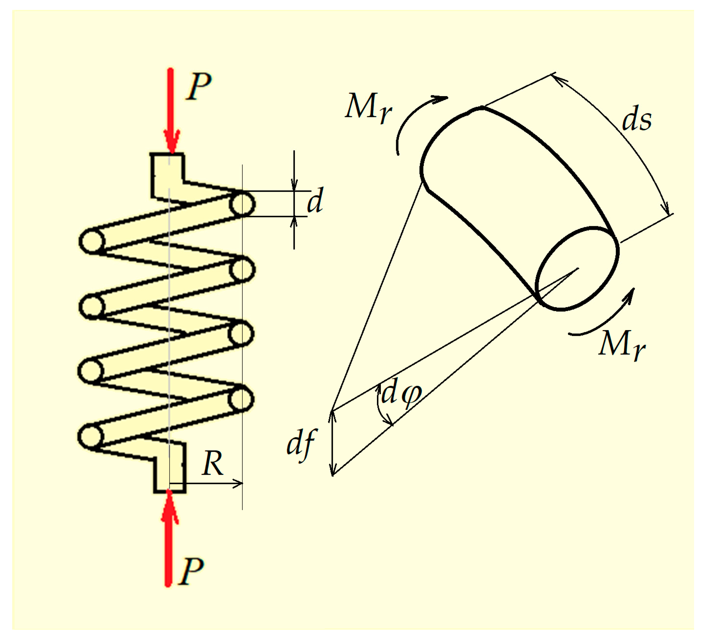
3.3. Calculation of a Helical Spring
3.4. Bending
- (a)
- Bending is treated using the assumptions of linear elasticity. Taking into account Bernoulli’s hypothesis, the elongation of a fiber located at a distance (y) from the neutral axis is deduced. It is found (Figure 9) that
- (b)
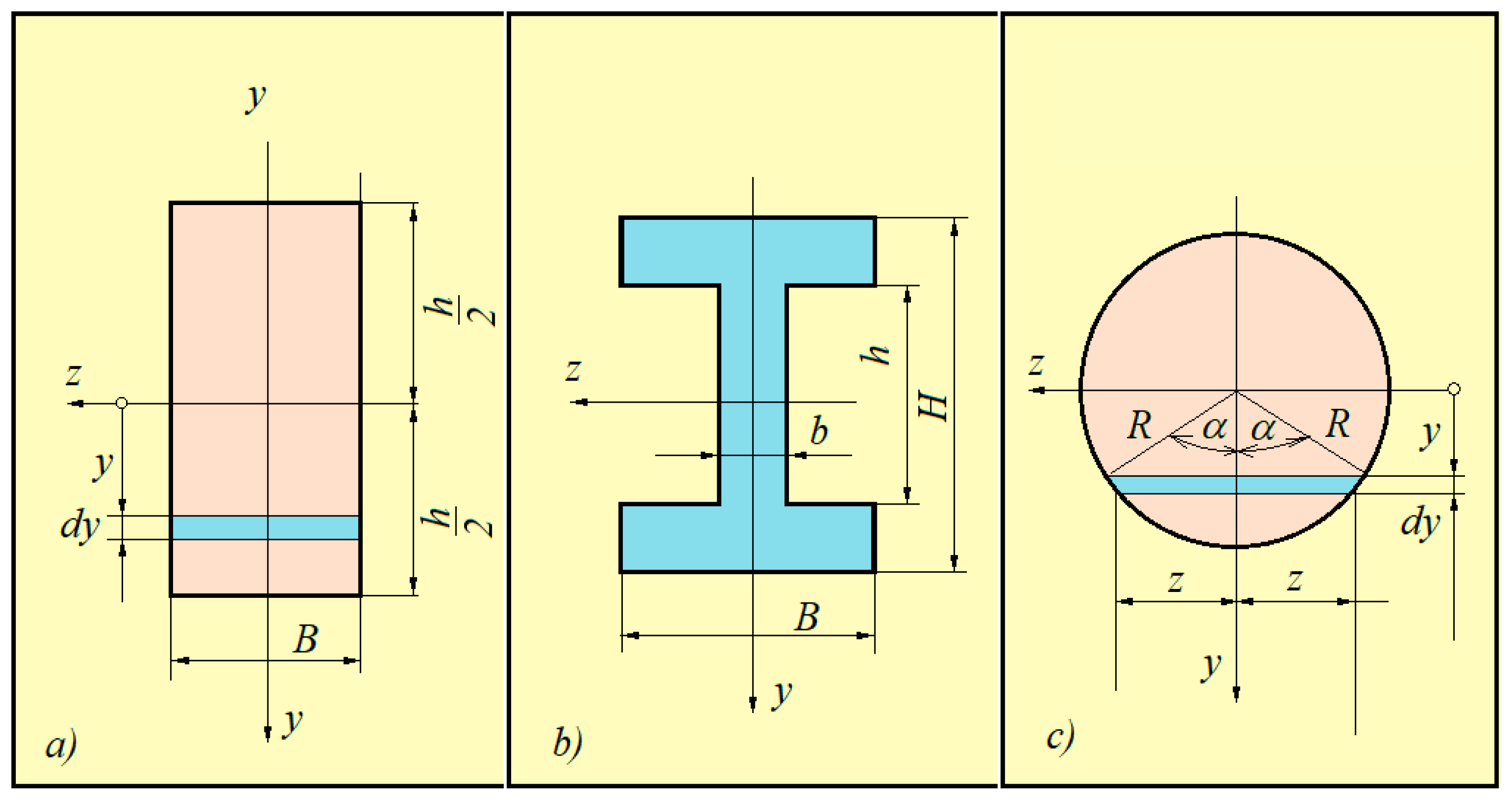
- and are calculated below for some sections that are often used in practice:
- n = 1: ;
- n = 1/2: ;
- n = 1/3: ;
- n = : .
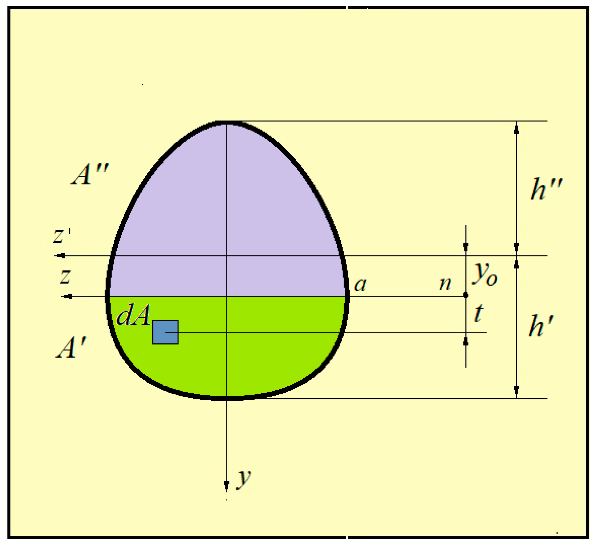
3.5. Inclined Bending
- (a)
- In the region A’,varies between 0 and :and
- (b)
- In the region A”,varies between and :and
3.6. Bending with Traction
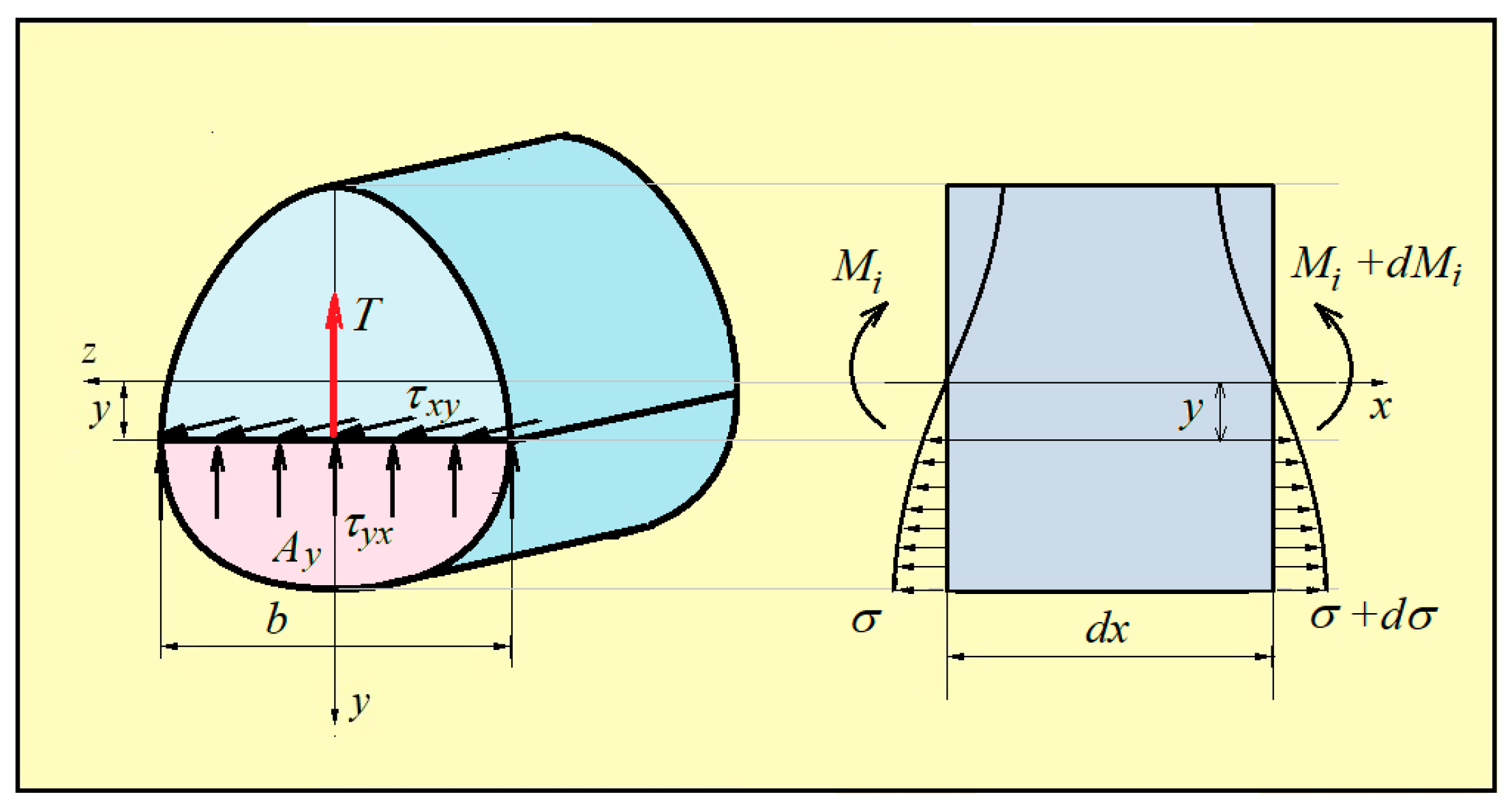
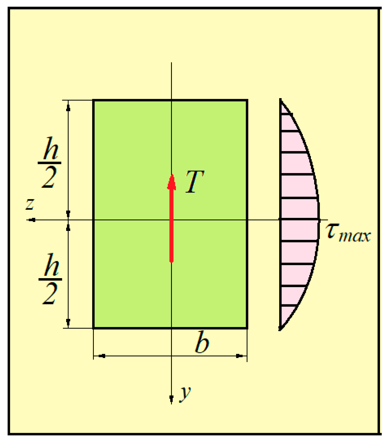
3.7. Shear
4. Conclusions
Author Contributions
Funding
Data Availability Statement
Conflicts of Interest
References
- Drapaca, C.S.; Sivaloganathan, S.; Tenti, G. Nonlinear constitutive laws in viscoelasticity. Math. Mech. Solids 2007, 12, 475–501. [Google Scholar] [CrossRef]
- Pruchnicki, E. Homogenized nonlinear constitutive law using Fourier series expansion. Int. J. Solids Struct. 1998, 35, 1895–1913. [Google Scholar] [CrossRef]
- Teferra, K.; Deodatis, G. Variability response functions for beams with nonlinear constitutive laws. Probabilistic Eng. Mech. 2012, 29, 139–148. [Google Scholar] [CrossRef]
- Michel, J.C.; Suquet, P. The Constitutive Law of Nonlinear Viscous and Porous Materials. J. Mech. Phys. Solids 1992, 40, 783–812. [Google Scholar] [CrossRef]
- Fatehiboroujeni, S.; Palanthandalam-Madapusi, H.J. Computational Rod Model With User-Defined Nonlinear Constitutive Laws. J. Comput. Nonlinear Dyn. 2018, 13, 101006. [Google Scholar] [CrossRef]
- Lainé, E.; Vallée, C.; Fortuné, D. Nonlinear isotropic constitutive laws: Choice of the three invariants, convex potentials and constitutive inequalities. Int. J. Eng. Sci. 1999, 37, 1927–1941. [Google Scholar] [CrossRef]
- Randall, N.M.; Ghorashi, M. AC 2012-2971: Design Manufacture Simulation and Expermentation of several Tools to Assist in Teaching Strength of Materials and SAtatics Courses. In Proceedings of the ASEE Annual Conference, San Antonio, TX, USA, 10–13 June 2012. [Google Scholar]
- Yang, Y.B.; Leu, L.J. Constitutive Laws and Force Recovery Procedures in Nonlinear-Analysis of Trusses. Comput. Methods Appl. Mech. Eng. 1991, 92, 121–131. [Google Scholar] [CrossRef]
- Mrówczynski, D.; Gajewski, T.; Garbowski, T. Application of the generalized nonlinear constitutive law in 2D shear flexible beam structures. Arch. Civ. Eng. 2021, 67, 157–176. [Google Scholar]
- Pavazza, R.; Jovic, S. A comparison of approximate analytical methods and the finite element method in the analysis of short clamped thin-walled beams subjected to bending by uniform loads. Trans. FAMENA 2007, 31, 37–54. [Google Scholar]
- Marin, M.; Carrera, E.; Vlase, S. An extension of the Hamilton variational principle for piezoelectric bodies with dipolar structure. Mech. Adv. Mater. Struct. 2023, 30, 2453–2457. [Google Scholar] [CrossRef]
- Zhang, H.W.; Shen, Y.; Zhang, S.W. To Solve the Load of Beam by Shearing Force Diagram and Bending Moment Diagram-Reverse Thinking in Strength of Materials. In Proceedings of the International Conference on Advanced Engineering Materials and Architecture Science (ICAEMAS 2014), Huhhot, China, 26–27 July 2014; pp. 546–549. [Google Scholar]
- Codarcea-Munteanu, L.; Marin, M.; Vlase, S. The study of vibrations in the context of porous micropolar media thermoelasticity and the absence of energy dissipation. J. Comput. Appl. Mech. 2023, 54, 437–454. [Google Scholar]
- Giménez-Palomares, F.; Jiménez-Mocholí, A.J.; Espinós-Capilla, A. Obtaining Stress Distribution in Bending through Virtual Laboratories. In Proceedings of the 8th International Technology, Education and Development Conference (INTED), Valencia, Spain, 10–12 March 2014; pp. 6209–6218. [Google Scholar]
- Katouzian, M.; Vlase, S.; Marin, M. Elastic moduli for a rectangular fibers array arrangement in a two phases composite. J. Comput. Appl. Mech. 2024, 55, 538–551. [Google Scholar]
- Fattal, R.; Kupferman, R. Constitutive laws for the matrix-logarithm of the conformation tensor. J. Non-Newton. Fluid Mech. 2004, 123, 281–285. [Google Scholar] [CrossRef]
- Yang, Q.S.; Xu, F. Numerical modeling of nonlinear deformation of polymer composites based on hyperelastic constitutive law. Front. Mech. Eng. 2009, 4, 284–288. [Google Scholar] [CrossRef]
- Braun, M.; Bishoff, M.; Ramm, E. Nonlinear Shell Formulations for Complete 3-Dimensional Constitutive Laws including Composites and Laminates. Comput. Mech. 1994, 15, 1–18. [Google Scholar] [CrossRef]
- Kim, J.H.; Lee, M.G.; Kang, T.J. Development of nonlinear constitutive laws for anisotropic and asymmetric fiber reinforced composites. Polym. Compos. 2008, 29, 216–228. [Google Scholar] [CrossRef]
- Bardella, L. A phenomenological constitutive law for the nonlinear viscoelastic behaviour of epoxy resins in the glassy state. Eur. J. Mech. A-Solids 2001, 20, 907–924. [Google Scholar] [CrossRef]
- Cai, W.; Wang, P.; Wang, Y.J. Linking fractional model to power-law constitutive model with applications to nonlinear polymeric stress-strain responses. Mech. Time-Depend. Mater. 2023, 27, 875–888. [Google Scholar] [CrossRef]
- Katouzian, K.; Vlase, S.; Scutaru, M.L. Finite Element Method-Based Simulation Creep Behavior of Viscoelastic Carbon-Fiber Composite. Polymers 2021, 13, 1017. [Google Scholar] [CrossRef] [PubMed]
- Scutaru, M.L.; Teodorescu-Draghicescu, H.; Vlase, S.; Marin, M. Advanced HDPE with increased stiffness used for water supply networks. J. Optoelectron. Adv. Mater. 2015, 17, 484–488. [Google Scholar]
- Hilton, H.H. Sensitivity Analysis for Viscoelastic Strength of Materials and Corresponding Continuum Mechanics Formulations. In Proceedings of the ASME International Mechanical Engineering Congress and Exposition, Boston, MA, USA, 31 October–6 November 2008; Published in 2009. Volume 1, pp. 95–110. [Google Scholar]
- Lolic, D.; Zupan, D.M. A consistent finite element formulation for laminated composites with nonlinear interlaminar constitutive law. Compos. Struct. 2020, 247, 112445. [Google Scholar] [CrossRef]
- Betsch, P. Nonlinear Finite Shell Element for Implementation of General 3D Constitutive Laws. Z. Fur Angew. Math. Mech.—Appl. Math. Mech. 1995, 75 (Suppl. S1), S245–S246. [Google Scholar]
- Goyal, V.K.; Johnson, E.R.; Dávila, C.G. Irreversible constitutive law for modeling the delamination process using interfacial surface discontinuities. Compos. Struct. 2004, 65, 289–305. [Google Scholar] [CrossRef]
- Cai, L.; Zhang, R.H.; Li, Y.Q.; Zhu, G.Y.; Ma, X.S.; Wang, Y.H.; Luo, X.Y.; Gao, H. The Comparison of Different Constitutive Laws and Fiber Architectures for the Aortic Valve on Fluid-Structure Interaction Simulation. Front. Physiol. 2012, 15, 131–140. [Google Scholar] [CrossRef] [PubMed]
- Dusi, A.; Bettinali, F.; Rebecchi, V.; Bonacina, G. High Damping Laminated Rubber Bearings (HDLRBs): A simplified non-linear model with exponential constitutive law—Model description and validation through experimental activities. In Proceedings of the 1st European Conference on Constitutive Models for Rubber, SEP 09-10, Vienna, Austria, 9–10 September 1999; pp. 229–235. [Google Scholar]
- Sansour, C.; Kollmann, F.G. Large viscoplastic deformations of shells. Theory and finite element formulation. Comput. Mech. 1998, 21, 512–525. [Google Scholar] [CrossRef]
- Teodorescu-Draghicescu, H.; Stanciu, A.; Vlase, S.; Scutaru, M.L.; Calin, M.R.; Serbina, L. Finite element method analysis of some fibre-reinforced composite laminates. Optoelectron. Adv. Mater.-Rapid Commun. 2011, 5, 782–785. [Google Scholar]
- Marin, M.; Agarwal, R.P.; Mahmoud, S.R. Modeling a microstretch thermo-elastic body with two temperatures. Abstr. Appl. Anal. 2013, 2013, 583464. [Google Scholar] [CrossRef]
- Wang, C.; Zhang, W.; Kassab, G.S. The validation of a generalized Hooke’s law for coronary arteries. Am. J. Physiol.-Heart Circ. Physiol. 2008, 294, H66–H73. [Google Scholar] [CrossRef] [PubMed]
- May-Newman, K.; Yin, F.C.P. A constitutive law for mitral valve tissue. J. Biomech. Eng.-Trans. ASME 1998, 120, 38–47. [Google Scholar] [CrossRef] [PubMed]
- Caggiano, L.R.; Holmes, J.W. A Comparison of Fiber Based Material Laws for Myocardial Scar. J. Elast. 2021, 145, 321–337. [Google Scholar] [CrossRef] [PubMed]
- Marcucci, L.; Bondi, M.; Randazzo, G.; Reggiani, C.; Natali, A.; Pavan, P.G. Fibre and extracellular matrix contributions to passive forces in human skeletal muscles: An experimental based constitutive law for numerical modelling of the passive element in the classical Hill-type three element model. PLoS ONE 2019, 14, e0224232. [Google Scholar] [CrossRef] [PubMed]
- Agarwal, A. An improved parameter estimation and comparison for soft tissue constitutive models containing an exponential function. Biomech. Model. Mechanobiol. 2017, 16, 1309–1327. [Google Scholar] [CrossRef] [PubMed]
- Feng, P.C.; Ma, H.C.; Wang, J.P.; Qian, J.Z.; Luo, Q.K. Influence mechanism of confining pressure on the hydraulic aperture based on the fracture deformation constitutive law. Front. Earth Sci. 2023, 10, 968696. [Google Scholar] [CrossRef]
- Rong, G.; Huang, K.; Zhou, C.B.; Wang, X.J.; Peng, L. A new constitutive law for the nonlinear normal deformation of rock joints under normal load. Sci. China-Technol. Sci. 2012, 55, 555–567. [Google Scholar] [CrossRef]
- Sgobba, S.; Geibel, B.; Blum, W. On the Constitutive Laws of Plastic-Deformation of INP Single-Crystals at High-Temperatures. Phys. Status Solidi A-Appl. Res. 1993, 137, 363–379. [Google Scholar] [CrossRef]
- Marin, M.; Öchsner, A.; Bhatti, M.M. Some results in Moore-Gibson-Thompson thermoelasticity of dipolar bodies. ZAMM-J. Appl. Math. Mech. 2020, 100, e202000090. [Google Scholar] [CrossRef]
- Marin, M.; Hobiny, S.; Abbas, I. Finite element analysis of nonlinear bioheat model in skin tissue due to external thermal sources. Mathematics 2021, 9, 1459. [Google Scholar] [CrossRef]
- Tan, Y.Z.; Shi, X.M.; Cheng, Y.H.; Li, G.; Yue, S.L.; Wang, M.Y.; Wang, Y.H.; Wang, P.Y.; Zhou, J.W. Research on the Damage Evolution Law and Dynamic Damage Constitutive Model of High-Performance Equal-Sized-Aggregate Concrete Materials. J. Mater. Civ. Eng. 2022, 34, 04022039. [Google Scholar] [CrossRef]
- Zidek, R.A.E.; Völlmecke, C. On the influence of material non-linearities in geometric modeling of kink band instabilities in unidirectional fiber composites. Int. J. Non-Linear Mech. 2014, 62, 23–32. [Google Scholar] [CrossRef]
- Nguyen, C. Analitic Model of Hydrodynamic Behavior uintil Cracking by Uniaxial Creep with Compacting. In Proceedings of the 3rd International Conf on Mechanical And Physical Behaviour of Materials Under Dynamic Loading (DYMAT 91), Strasbourg, France, 14–18 October 1991. [Google Scholar]
- Wang, J.T.; Wei, W.; Zhang, Y.; Chen, G. An investigation on softening in constitutive relationship of metals at high strain level. In Proceedings of the 4th International Symposium on Ultrafine Grained Materials, San Antonio, TX, USA, 12–16 March 2006; pp. 89–97. [Google Scholar]
- Vlase, S.; Marin, M.; Scutaru, M.L.; Munteanu, R. Coupled transverse and torsional vibrations in a mechanical system with two identical beams. AIP Adv. 2017, 7, 065301. [Google Scholar] [CrossRef]
- Ishfaq, K.; Asad, M.; Harris, M.; Alfaify, A.; Anwar, S.; Lamberti, L.; Scutaru, M.L. EDM of Ti-6Al-4V under Nano-Graphene Mixed Dielectric: A Detailed Investigation on Axial and Radial Dimensional Overcuts. Nanomaterials 2022, 12, 432. [Google Scholar] [CrossRef] [PubMed]
- Oshiro, R.E.; Alves, M. Scaling of structures subject to impact loads when using a power law constitutive equation. Int. J. Solids Struct. 2009, 46, 3412–3421. [Google Scholar] [CrossRef]
- Niculita, C.; Vlase, S.; Bencze, A.; Mihalcica, M.; Calin, M.R.; Serbina, L. Optimum stacking in a multi-ply laminate used for the skin of adaptive wings. Optoelectron. Adv.. Mater. -Rapid Commun. 2011, 5, 1233–1236. [Google Scholar]
- Kissas, G.; Mishra, S.; Chatzi, E.; De Lorenzis, L. The language of hyperelastic materials. Comput. Methods Appl. Mech. Eng. 2024, 428, 117053. [Google Scholar] [CrossRef]
- Imane, O.; Benyattou, B.; Yamna, B.; Baowei, F. On a dynamic frictional contact problem with normal damped response and long-term memory. Math. Mech. Solids 2024, 29, 924–943. [Google Scholar] [CrossRef]
- Sawada, K.; Tabuchi, M.; Kimura, K. Analysis of long-term creep curves by constitutive equations. In Proceedings of the 11th International Conference of Creep and Fracture of Engineering Materials and Structures, Bad Berneck, Germany, 4–9 May 2008; Volume 510–511, pp. 190–194. [Google Scholar] [CrossRef]
- Aharonov, E.; Scholz, C.H. The Brittle-Ductile Transition Predicted by a Physics-Based Friction Law. J. Geophys. Res. Solid Earth 2019, 124, 2721–2737. [Google Scholar] [CrossRef]
- Raj, S.V.; Freed, A.D. A phenomenological description of primary creep in class M materials. Mater. Sci. Eng. A-Struct. Mater. Prop. Microstruct. Process. 2000, 283, 196–202. [Google Scholar] [CrossRef]
- Fabrizio, M.; Lazzari, B.; Rivera, J.M. Asymptotic behaviour for a two-dimensional thermoelastic model. Math. Methods Appl. Sci. 2007, 30, 549–566. [Google Scholar] [CrossRef]
- Zhang, W.; Wang, C.; Kassab, G.S. The mathematical formulation of a generalized Hooke’s law for blood vessels. Biomaterials 2007, 28, 3569–3578. [Google Scholar] [CrossRef] [PubMed]
- Timoshenko, S. Elements of Strength of Materials, 5th ed.; Van Nostrand: New York, NY, USA, 1968. [Google Scholar]


Disclaimer/Publisher’s Note: The statements, opinions and data contained in all publications are solely those of the individual author(s) and contributor(s) and not of MDPI and/or the editor(s). MDPI and/or the editor(s) disclaim responsibility for any injury to people or property resulting from any ideas, methods, instructions or products referred to in the content. |
© 2024 by the authors. Licensee MDPI, Basel, Switzerland. This article is an open access article distributed under the terms and conditions of the Creative Commons Attribution (CC BY) license (https://creativecommons.org/licenses/by/4.0/).
Share and Cite
Vlase, S.; Marin, M. Standard Deformations of Nonlinear Elastic Structural Elements with Power-Law Constitutive Model. Mathematics 2024, 12, 3992. https://doi.org/10.3390/math12243992
Vlase S, Marin M. Standard Deformations of Nonlinear Elastic Structural Elements with Power-Law Constitutive Model. Mathematics. 2024; 12(24):3992. https://doi.org/10.3390/math12243992
Chicago/Turabian StyleVlase, Sorin, and Marin Marin. 2024. "Standard Deformations of Nonlinear Elastic Structural Elements with Power-Law Constitutive Model" Mathematics 12, no. 24: 3992. https://doi.org/10.3390/math12243992
APA StyleVlase, S., & Marin, M. (2024). Standard Deformations of Nonlinear Elastic Structural Elements with Power-Law Constitutive Model. Mathematics, 12(24), 3992. https://doi.org/10.3390/math12243992