Adaptive Centroid-Connected Structure Matching Network Based on Semi-Supervised Heterogeneous Domain

Abstract

Heterogeneous domain adaptation (HDA) utilizes the knowledge of the source domain to model the target domain. Although the two domains are semantically related, the problem of feature and distribution differences in heterogeneous data still needs to be solved. Most of the existing HDA methods only consider the feature or distribution problem but do not consider the geometric semantic information similarity between the domain structures, which leads to a weakened adaptive performance. In order to solve the problem, a centroid connected structure matching network (CCSMN) approach is proposed, which firstly maps the heterogeneous data into a shared public feature subspace to solve the problem of feature differences. Secondly, it promotes the overlap of domain centers and nodes of the same category between domains to reduce the positional distribution differences in the internal structure of data. Then, the supervised information is utilized to generate target domain nodes, and the geometric structural and semantic information are utilized to construct a centroid-connected structure with a reasonable inter-class distance. During the training process, a progressive and integrated pseudo-labeling is utilized to select samples with high-confidence labels and improve the classification accuracy for the target domain. Extensive experiments are conducted in text-to-image and image-to-image HDA tasks, and the results show that the CCSMN outperforms several state-of-the-art baseline methods. Compared with state-of-the-art HDA methods, in the text-to-image transfer task, the efficiency has increased by 8.05%; and in the image-to-image transfer task, the efficiency has increased by about 2%, which suggests that the CCSMN benefits more from domain geometric semantic information similarity.

1. Introduction

Traditional machine learning methods have achieved remarkable success due to the availability of various large-scale datasets [1,2,3,4,5,6], for example, ImageNet [7]. However, training a model using a large amount of labeled data is time-consuming and laborious, as obtaining labels is relatively difficult. One possible solution is to utilize a similar and sufficiently labeled domain to help train out a model for another domain. However, the distribution differences exist in different fields, which can easily lead to training failure. Transfer learning [8,9,10,11,12] has been widely used as a feasible technique to solve the problem of insufficient training data and data distribution differences.

Among transfer learning methods, domain adaptation (DA) [13,14,15,16] is widely used because it reduces the requirement for data distribution, i.e., the marginal and conditional distributions between the source domain and target domain can be different. DA has been used in computer vision, natural language processing, speech recognition [17,18,19], etc. DA can be divided into homogeneous and heterogeneous domain adaptation. Most of the current work is homogeneous domain adaptation, which restricts the problem to the condition of homogeneity, i.e., the source and target domains have the same feature dimensions and feature representations, but they are different in distribution [20,21,22]. However, what if the source and target domains are more heterogeneous, and their feature spaces and data distributions are heterogeneous? For example, the source domain is composed of text, but the target domain is composed of images, or both the domains are image data, but they are are composed of different features extracted by different neural network models (e.g., SURF and DECAF), as shown in Figure 1.

In order to address the aforementioned heterogeneous migration task, domain adaptation has been extended to heterogeneous domains (HDA), but the primary problem to be solved is that the two domains have feature representations with different dimensions. The existing feature transformation methods are mainly divided into two types: one is to construct a common subspace from the two domains [23,24,25], and the other is to project the data from one domain to the other [26,27,28,29]. After feature transformation, the mainstream approach is to minimize the difference in data distribution [29,30]. Some researchers focus on optimizing the discriminative ability of the classifier with source domain knowledge [31,32,33].

Although previous methods have been successful and have focused on domain alignment, the inherent geometric structure information has not been taken into consideration. Therefore, the centroid connectivity structure and the semantic information are ignored, which leads to the models not being able to distinguish samples of different categories, resulting in the low generalization performance of classifiers in the target domain. In addition, some heterogeneous domain adaptation methods only train individual classifiers in the source domain, which can easily make incorrect predictions.

In order to overcome the limitations of previous HDA methods, a centroid-connected structure matching network is proposed to solve the semi-supervised heterogeneous domain adaptation problem. By constructing two centroid-connected structures, the semantic information in the source is transmitted to the target domain as much as possible, so that the two centroid-connected structures are perfectly aligned and the adaptive effect is improved. Firstly, a feature encoder is used to transform the features into a public feature subspace, and a prototype network [34] is used to normalize the features [35,36,37,38] so that heterogeneous data have the same feature dimension and achieve better structural alignment results. Secondly, reusing the labeled source and target domains to generate two centroid-connected structures, the pseudo-label joint decision-making mechanism is used to assign high-reliability pseudo-labels to unlabeled target samples. Lastly, the position distribution alignment of the structure is achieved through the domain center rotation mechanism and node attraction mechanism. At the same time, a node semantic and structure semantic sharing mechanism is used to dynamically optimize the target structure to promote the overlap of the two structures. Overall, the contributions of this paper are as follows:

• A novel centroid-connected structure matching network (CCSMN) is proposed to generate a complete and accurate target domain based on the geometric properties of the data, which is generated by the labeling information of the source and target domains to facilitate the positional distribution of the structures to be aligned;
• Deeply mining the geometric semantic information when aligning two centroid-connected structures, it ensures that the semantic information and the structure of the target domain have a reasonable category distance and reduces the structural discrepancy;
• Extensive experiments on benchmark datasets show that the proposed framework CCSMN is more competitive than the state-of-the-art methods.

The remainder of the paper is organized as follows. Section 2 presents an overview of related work. Section 3 defines the problem and presents the details of the proposed approach. Section 4 presents the experiments results. Finally, conclusions are drawn and future work suggested in Section 5.

2. Related Work

Heterogeneous domain adaptation (HDA) [27,39] needs to solve the difference between the feature spaces of the source and target domains. Most HDAs use the following two dominant feature transformation methods to reduce domain bias due to data heterogeneity. One is the cross-domain unidirectional feature transformation method, and the other is the standard subspace feature transformation method.

(1)

Cross-domain unidirectional feature transformation methods: Mapping data from one domain to another using a mapping function. Kulis et al. [27] design an asymmetric regularized cross-domain transform to learn asymmetric and nonlinear transformations to map data across domains. However, it ignores category information, including the geometric structure and conditional distributions. Tsai [28] proposes a cross-domain landmark selection algorithm to select representative cross-domain data to reduce domain bias. It only aligns the cross-domain statistical distributions, and its feature transformation causes inadequate feature information. Yao [29] proposes a conditional weighting adversarial network (CWAN) to learn a feature transformer, a label classifier, and a domain discriminator. To quantify the importance of different source domains, the CWAN introduces a sophisticated conditional weighting funciton to calculate the weights of the source domains according to the conditional distribution divergence between the source and target domains. Obrenovic et al. [30] propose a maximum spaced domain transformation method to map the target data to the source domain, which can be co-optimized with the classifiers.

(2)

Public Subspace Feature Transformation Methods: Both domains are mapped to a public subspace. Mori et al. [31] propose a naive combination of existing positive and unlabeled DA learning methods to predict likely positive examples from the unlabeled target data and simultaneously align the feature space. Chen et al. [32] propose a novel HDA method called class centroid matching and local discriminative structure preservation (CMDP), which can transfer discriminative semantic source knowledge to the target domain. Specifically, it projects cross-domain samples to regress the label matrix, to align the discriminative directions of two domains and introduce the inner product strategy, so as to align the distance and angle of the class centroids across domains. Li et al. [33] proposed a locality-preserving joint transfer method which combines distribution matching, landmark selection, and local consistency and predicts labels using label propagation. Later, they proposed independent transfer [34], which optimizes the geometric relationships of the samples by learning multiple transformations and using graph-based landmark selection. But the two domains miss some critical information when features are transformed into the subspace. Alipour et al. [35] propose statistical distribution alignment and progressive pseudo-label selection for heterogeneous domain adaptation (SDA-PPLS). However, SDA-PPLS with pseudo-label selection is not a more optimal integration prediction method.

Although all of these HDA methods are effective, none of them take into account intrinsic geometric structural properties. They neglect to construct the matching network from a geometric perspective and do not delve into the structural–semantic information contained in intrinsic geometric structural properties. In addition, the failure to assign high-confidence pseudo-labels to unlabeled target domains results in no further improvement in the performance of their models.

The centroid-connected structure matching network proposed in this paper is based on the assumption that a domain-invariant subspace exists, with one prototype for each class, and the data of the same class are projected around their respective prototypes. Using the prototype network [36,37] can approximate the distribution of each class and enable one to realize that the prototypes are close to each other in the subspace. Nguyen et al. [38] normalize the feature representation based on the prototype network. Taekyung [39] embeds all normalized features of prototypes and samples in a spherical feature space to achieve the alignment of data distributions across domains.

However, previous prototype works do not consider the HDA. Distinct from this previous work, a centroid-connected structure is constructed for the source and target domains, respectively. It considers the semantic information of a single node in the source domain, which guides the generation of the same category of nodes in the target domain. In addition, the semantic information between different nodes in the source domain can help the overall structure of the target domain to be more explicit and perfect, and realize the perfect alignment of the cross-domain structure from the global to the local with the coarse-grained to the fine-grained level, and improve the adaptive performance.

3. The Proposed Approach

3.1. Notation

In the semi-supervised HDA, there is a source domain and a target domain. Specifically, the labeled source domain is ${\mathcal{D}}_S=\left\{{\mathcal{X}}_S, {\mathcal{Y}}_S\right\}={\left\{\left(x_s^i,y_s^i\right)\right\}}_{i=1}^{n_s}$, where $x_s^i\in {ℝ}^{d_s}$ denotes the $i$th sample of the source domain and there are $n_s$ source samples; and $y_s^i$∈{1, …, K} denotes the corresponding label, K is the number of categories of labels, and the feature dimensions of the source sample are $d_s$. The few labeled target domains are ${\mathcal{D}}_T=\left\{{\mathcal{X}}_T, {\mathcal{Y}}_T\right\}={\mathcal{D}}_{TL}\cup {\mathcal{D}}_{TU}$, ${\mathcal{D}}_{TL}=\left\{{\mathcal{X}}_L,{\mathcal{Y}}_L\right\}={\left\{\left(x_l^i,y_l^i\right)\right\}}_{i=1}^{n_l}, {\mathcal{D}}_{TU}=\left\{{\mathcal{X}}_U\right\}={\left\{\left(x_u^i\right)\right\}}_{i=1}^{n_u}$, where $x_l^i\in {ℝ}^{d_t}$ denotes the $i$th labeled target sample and there are $n_l$ labeled target samples; the feature dimensions of the target sample are $d_t$. Note that setting $n_s\gg n_l,n_u\gg n_l$ and $d_s\ne d_t$.

Table 1. Notations.

Notation	Definition
${\mathcal{D}}_S$/${\mathcal{D}}_T$	Source/target domain
${\mathcal{X}}_S/{\mathcal{Y}}_S$	Source data/labels
${\mathcal{X}}_T/{\mathcal{Y}}_T$	Target data/labels
${\mathcal{X}}_L/{\mathcal{Y}}_L$	Target labeled data/labels
${\mathcal{X}}_U$/${\mathcal{Y}}_U$/${\widehat{\mathcal{Y}}}_U$	Target unlabeled data/true labels/pseudo-labels
${\mathcal{H}}_S$/${\mathcal{H}}_T$	Normalized source/target data
${\mathcal{H}}_L$/${\mathcal{H}}_U$	Normalized target labeled/unlabeled data
$h_s^i/h_t^i$	$i^{th}$ normalized source/target data
$h_l^i/h_u^i$	$i^{th}$ normalized target labeled/unlabeled data
$n_s/n_l/n_u$	Number of source/labeled target/unlabeled target
$d_s/d_t$	Dimension of source/target data
$x_s^i/y_s^i$	$i^{th}$ source data/label
$x_t^i/y_t^i$	$i^{th}$ target data/label
$x_l^i/y_l^i$	$i^{th}$ labeled target data/label
$x_u^i$	$i^{th}$ unlabeled target data
${\mathsf{\Omega }}_S/{\mathsf{\Omega }}_T$	Feature encoder for source/target domain
${\overline{\mathcal{W}}}_S/{\overline{\mathcal{W}}}_T$	Center of source domain/target domain
${\overline{\mathcal{W}}}_S^k/{\overline{\mathcal{W}}}_T^k$	Center of source domain/target domain in class K
${\overline{\mathcal{H}}}_S^k/{\overline{\mathcal{H}}}_T^k$	Center of normalized source domain/target domain in class K
T	Temperature hyperparameter
$d_{com}$	Subspace dimension
$\alpha ,\beta ,\delta , \lambda$	Tradeoff parameters

is the notations and its descriptive definitions.

3.2. Framework of CCSMN

The centroid-connected structures of the labeled source and the target domains with little labeled data maintain their original structural shapes at different locations in the same feature space, and there are positional distributional differences and structural differences, which result in the inability to achieve overlap. To make them coincide, the feature differences between the domains are resolved by using two feature encoders with three-layer neural networks to map the heterogeneous data into a subspace with the same feature dimension. Normalization methods process the features in the subspace. Then, the positional distributions are aligned using domain center rotation and node attraction mechanisms. To mine the geometric semantic information, the node semantic sharing mechanism and the structural–semantic sharing mechanism are designed to realize the points for the generation of the overall structure from coarse-grained to fine-grained, which ensures semantic purity and realizes the aggregation of the nodes within the class and the separability between the classes, and helps to align the cross-domain structure. For unlabeled target domain data, a progressive pseudo-labeling co-decision mechanism combines neural network prediction to select samples with high-confidence pseudo-labels to be added to the training process, thereby improving the classification performance. A domain-invariant and distinguishable feature encoder and a domain-sharing classifier F(·) can be trained by the joint action framework. The framework of the proposed method is shown in Figure 2.

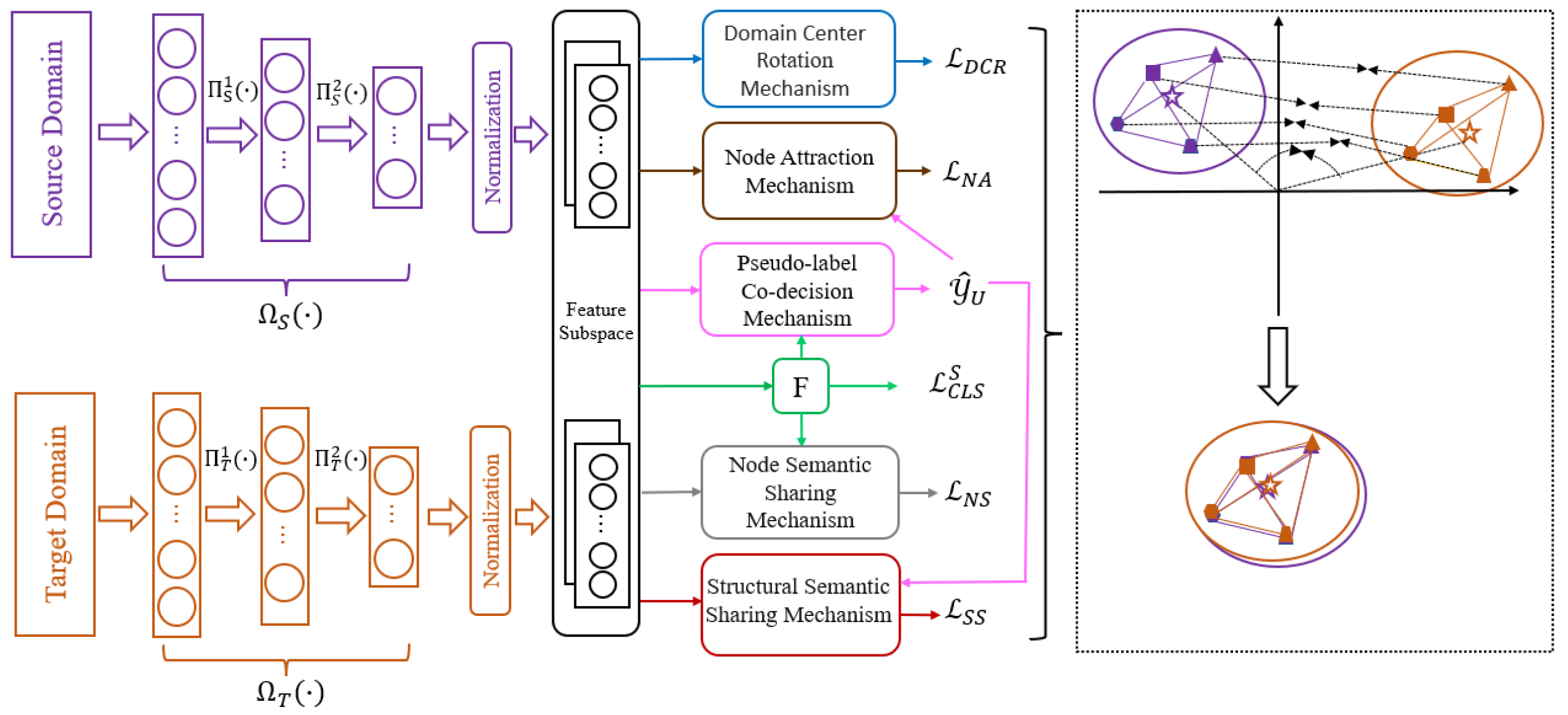
3.3. Centroid-Connected Structure Matching Network

(1) Feature Representation

Due to the different feature representations and dimensions of the source and target domain data, the learned classification model cannot be directly applied to the target domain. To solve the problem, a shared public feature subspace needs to be constructed. Firstly, a standard feature subspace learning network is constructed for the source and target domains, respectively, which contains two feature encoders ${\mathsf{\Omega }}_S\left(x_s^i\right)={\mathsf{\Pi }}_S^2\left({\mathsf{\Pi }}_S^1\left(x_s^i\right)\right)$, where $x_s^i\in {\mathcal{X}}_S$ and ${\mathsf{\Omega }}_T\left(x_t^i\right)={\mathsf{\Pi }}_T^2\left({\mathsf{\Pi }}_T^1\left(x_t^i\right)\right)$ and where $x_t^i\in {\mathcal{X}}_T$ and ${\mathcal{X}}_T={\mathcal{X}}_L\cup {\mathcal{X}}_U$. The two feature encoders can embed heterogeneous data into a domain-invariant feature space, and both of them consist of a three-layer neural network. ${\mathsf{\Pi }}_S^1\left(·\right)$ and ${\mathsf{\Pi }}_T^1\left(·\right)$ are the transformation functions between the input and intermediate layers, and ${\mathsf{\Pi }}_S^2\left(·\right)$ and ${\mathsf{\Pi }}_T^2\left(·\right)$ are the transformation functions between the intermediate and output layers. The dimensions of the three-layer network of the feature encoders are $d_s^1, d_s^2, d_s^3$ and $d_t^1, d_t^2$, $d_t^3$ respectively. The input layer dimensions $d_s^1$ and $d_t^1$ of the two feature encoders are set to be equal to the feature dimensions of the input samples of the source and target domains, respectively, and the output layer dimensions $d_s^3$ and $d_t^3$ are set to be equal to the dimensions of the feature space $d_{com}$. That is, $d_s^3$ = $d_t^3$ = $d_{com}$. In order to avoid the lack of effective feature information caused by the direct feature transformation [25,29,40,41] and to ensure deep feature information can be learned, the intermediate layer dimensions are set as $d_s^2=\lfloor (d_s^1$+$d_s^3$)/2⌋, $d_t^2=\lfloor (d_t^1$+$d_t^3$)/2⌋, where $\lfloor ·\rfloor$ denotes a downward rounding operation. After learning the feature space, the transformed source domain feature ${\mathcal{W}}_S={\mathsf{\Omega }}_S\left({\mathcal{X}}_S\right)\in {ℝ}^{n_s\times d_{com}}$, $w_s^i$ is the $i$th sample feature of ${\mathcal{W}}_S$, and similarly, the transformed target domain feature ${\mathcal{W}}_T={\mathsf{\Omega }}_T\left({\mathcal{X}}_T\right)\in {ℝ}^{n_t\times d_{com}}$, $w_t^i$ is the $i$th sample of ${\mathcal{W}}_T={\mathcal{W}}_L\cup {\mathcal{W}}_U$ features. By learning the feature space, a new shared feature representation is obtained, which helps knowledge transfer to the target domain.

(2) Basic concepts

A centroid-connected structure is constructed for each domain separately to realize the alignment across domains. The three basic concepts are given below:

Domain center: the centroid of the source or target domain in the standard feature subspace;

Node: the centroid of category k set of the source or target domain;

Point distance: the weight of the domain centers or between any two nodes, measured by the square of the Euclidean distance.

The expression for the domain center is given in Equation (1):

$${\overline{\mathcal{W}}}_S={\displaystyle \frac{1}{{|}_{{\mathcal{X}}_S}|}}{{\displaystyle \sum }}_{x_s^i\in {\mathcal{X}}_S}{\mathsf{\Omega }}_S\left(x_s^i\right)={\displaystyle \frac{1}{{|}_{{\mathcal{X}}_S}|}}{{\displaystyle \sum }}_{x_s^i\in {\mathcal{X}}_S}{w}_s^i,{\overline{\mathcal{W}}}_T={\displaystyle \frac{1}{{|}_{{\mathcal{X}}_T}|}}{{\displaystyle \sum }}_{x_s^i\in {\mathcal{X}}_T}{\mathsf{\Omega }}_T\left(x_T^i\right)={\displaystyle \frac{1}{{|}_{{\mathcal{X}}_T}|}}{{\displaystyle \sum }}_{x_t^i\in {\mathcal{X}}_T}{w}_t^i$$

(1)

where |·| is the number of samples in the set.

The node representations of the source and target domains are shown in Equation (2):

$${\overline{\mathcal{W}}}_S^k={\displaystyle \frac{1}{{|}_{{\mathcal{W}}_S^k}|}}{{\displaystyle \sum }}_{w_s^i\in {\mathcal{W}}_S^k}{w}_s^i, {\overline{\mathcal{W}}}_T^k={\displaystyle \frac{1}{{|}_{{\mathcal{W}}_T^k}|}}{{\displaystyle \sum }}_{w_t^i\in {\mathcal{W}}_T^k}{w}_t^i,k\in \left\{1,2,\dots ,K\right\}$$

(2)

where K is the number of all categories and the number of nodes per domain.

(3) Domain center rotation mechanism

Considering the heterogeneous features are interconnected in the mapping space, the probability distributions still have a large divergence. Unlike the simple normalization in [41,42], the CCSMN does not directly minimize the distance between the two domain centers (${\overline{\mathcal{W}}}_S$ and ${\overline{\mathcal{W}}}_T$) to solve the angular difference. Instead, the source and the target domain features are normalized with the center of ${\overline{\mathcal{W}}}_S$ based on Equation (1), and the inter-domain difference in the mapping space is reduced through a unified scale, as in Equation (3).

$$h_s^i={\displaystyle \frac{w_s^i-{\overline{\mathcal{W}}}_S}{\parallel w_s^i-{\overline{\mathcal{W}}}_S{\parallel }_2}}, h_t^i={\displaystyle \frac{w_t^i-{\overline{\mathcal{W}}}_S}{\parallel w_t^i-{\overline{\mathcal{W}}}_S{\parallel }_2}}$$

(3)

where $\parallel ·{\parallel }_2$ is ${\mathcal{l}}^2$-normalize, ${\overline{\mathcal{W}}}_S$ is the initial centroid of the source domain, $h_s^i\in {\mathcal{H}}_S$, $h_t^i\in {\mathcal{H}}_T={\mathcal{H}}_L\cup {\mathcal{H}}_U$, $h_l^i\in {\mathcal{H}}_L$, $h_u^i\in {\mathcal{H}}_U$, $h_s^i$ and $h_t^i$ are the normalized source and target domain features of $w_s^i$ and $w_t^i$, respectively, and $h_l^i$ and $h_u^i$ are labeled and unlabeled features normalized to the target domain. Then the centroid, i.e., the domain center, of the entire feature space after normalization is recalculated according to Equation (4).

$${\overline{\mathcal{H}}}_S={\displaystyle \frac{1}{{|}_{{\mathcal{H}}_S}|}}{{\displaystyle \sum }}_{h_s^i\in {\mathcal{H}}_S}{h}_s^i,{\overline{\mathcal{H}}}_T={\displaystyle \frac{1}{{|}_{{\mathcal{H}}_T}|}}{{\displaystyle \sum }}_{h_t^i\in {\mathcal{H}}_T}{h}_t^i$$

(4)

There is an angular difference between the two structures. To be able to align the structures better, the structures are rotated by minimizing the loss in Equation (5) so that the angle between domain centers is 0 degrees, which completes the feature fusion between the global domains and avoids the angular difference of the structures in the global domain.

$${\mathcal{L}}_{DCR}=1-\mathsf{\Phi }\left({\overline{\mathcal{H}}}_S,{\overline{\mathcal{H}}}_T\right)$$

(5)

where $\mathsf{\Phi }\left(·,·\right)$ denotes the cosine similarity.

(4) Node attraction mechanism

The above mechanisms realize the global inter-domain alignment. It forces the angle between the domain centers to be zero. Still, it is a coarse-grained alignment that can only ensure an inevitable overlap of the geometric structure, and the nodes of different categories may be very close to each other. There is an overlap of the nodes of different categories. In contrast, if the nodes in the same category cannot overlap, this leads to negative transfer. To effectively reduce the appearance of negative transfer, this paper adopts the node attraction mechanism to further strengthen the node alignment between cross-domains, to complete the fine-grained coverage and calculate the nodes of category k in the source and target domains using Equation (6).

$${\overline{\mathcal{H}}}_S^k={\displaystyle \frac{1}{{|}_{{\mathcal{H}}_S^k}|}}{{\displaystyle \sum }}_{h_s^i\in {\mathcal{H}}_S^k}{h}_s^i, {\overline{\mathcal{H}}}_T^k={\displaystyle \frac{1}{{|}_{{\mathcal{H}}_T^k}|}}{{\displaystyle \sum }}_{h_t^i\in {\mathcal{H}}_T^k}{h}_t^i$$

(6)

Considering the existence of a large number of unlabeled target samples, inspired by [43], a pseudo-labeling strategy is used to assign pseudo-labels to each unlabeled target sample. Once the complete labeled target domain is obtained, the respective nodes can be constructed simultaneously with the labeled source domain. By minimizing the loss in Equation (7), the two structures are aligned in a finer way.

$${\mathcal{L}}_{NA}={\displaystyle \frac{1}{k}}{{\displaystyle \sum }}_{k=1}^K\mathsf{\Psi }\left({\overline{\mathcal{H}}}_S^k,{\overline{\mathcal{H}}}_T^k\right)={\displaystyle \frac{1}{k}}{{\displaystyle \sum }}_{k=1}^K\parallel {\overline{\mathcal{H}}}_S^k-{\overline{\mathcal{H}}}_T^k{\parallel }^2$$

(7)

where $\mathsf{\Psi }\left(·,·\right)={\parallel ·\parallel }^2$ is the square Euclidean distance. The node attraction mechanism can go a step further to effectively alleviate the problem of the difference, improve the utilization of the data in the process of knowledge transfer, fully explore the knowledge information, and help to improve the transfer performance.

(5) Node semantic sharing mechanism

The above two mechanisms in (4) focus on realizing the alignment of geometric structures from domain centers and nodes, which cannot effectively solve the problem of the difference in the shapes of the initial structures of the two domains. When aligning the whole geometric structure, it is necessary to ensure the consistency of the shapes of the two structures. Therefore, two semantic sharing mechanisms are designed to promote the target domain to generate a geometric structure shape as similar as possible to the source domain to make the structure alignment more accurate and efficient.

In a connected structure, each node has a corresponding category. Nodes in different domains belonging to the same category should exhibit a characteristic probabilistic category similarity in model prediction. Sharing the potential knowledge of the source domain with the target domain completes the first step of similar shape generation, facilitates the generation of nodes in the target domain, and ensures the meaning of the semantics. In detail, for a node of category k in the source domain, the potential knowledge it contains can be expressed as follows:

$$p^k={\displaystyle \frac{1}{{|}_{{\mathcal{H}}_S^k}|}}{{\displaystyle \sum }}_{h_s^i\in {\mathcal{H}}_S^k}softmax\left({\displaystyle \frac{F\left(h_s^i\right)}{T}}\right)$$

(8)

where T is a temperature hyperparameter that guarantees the smooth output of potential knowledge; for the source domain potential knowledge $p^k$ to be shared with the labeled samples in the target domain, the potential knowledge of the labeled target samples is also computed:

$$q_i=softmax\left(F\left(h_l^i\right)\right),h_l^i\in {\mathcal{H}}_L^k$$

(9)

where $H_L^k$ is the subset consisting of labeled target samples belonging to category k. Sharing potential knowledge and facilitatying the generation of target domain nodes by minimizing the loss in Equation (10),

$${\mathcal{L}}_{SKG}=-{\displaystyle \frac{1}{{|}_{{\mathcal{H}}_L}|}}{{\displaystyle \sum }}_{h_l^i\in {\mathcal{H}}_L,y_l^i\in {\mathcal{Y}}_L}{\left(p^{y_i}\right)}^{\mathsf{{\rm T}}}\log \left(q_i\right)$$

(10)

In addition, the supervised loss of labeled target domain samples is added, and the complete node semantic sharing loss is defined as

$${\mathcal{L}}_{NS}={\displaystyle \frac{1-\delta }{{|}_{{\mathcal{H}}_L}|}}{{\displaystyle \sum }}_{h_l^i\in {\mathcal{H}}_L,y_l^i\in {\mathcal{Y}}_L}{\mathcal{L}}_C\left(F\left(h_t^i\right),y_l^i\right)+\delta {\mathcal{L}}_{SKG}$$

(11)

where $\delta$ is the equilibrium hyperparameter of the loss ${\mathcal{L}}_{NS}$ and ${\mathcal{L}}_C$ is the cross-entropy loss. By minimizing the final loss ${\mathcal{L}}_{NS}$, the classification performance of the target domain is improved, the generation of target domain nodes is perfected, and the intra-class compactness of the nodes is achieved by ensuring the purity of semantics.

(6) Structural semantic sharing mechanism

The first step of similar shape generation through (5) emphasizes the probabilistic category similarity of nodes. It refines the generation of nodes in the target domain. Secondly, although there are a small number of labeled samples in the target domain, the semantics cannot generate a good structure for unlabeled samples, which is likely to make the nodes very close to each other. Therefore, a structure semantic sharing mechanism is designed, which mainly focuses on the semantic similarity of the overall structure, i.e., the semantic similarity between the nodes in the centroid-connected structure, and ensures that the target domain nodes have the same reasonable distinguishing distance from each other, and further generates a highly similar structure, which reduces the structural differences.

Specifically, the geometric semantic similarity between nodes in each domain, based on the relationship between nodes and domain centers, i.e., the semantic similarity between category node i and category node j, is calculated as follows:

$$\begin{array}{c}\hspace{1em}\hspace{1em}\mathsf{\Psi }\left({\mathcal{H}}_S^i-{\overline{\mathcal{H}}}_S,{\mathcal{H}}_S^j-{\overline{\mathcal{H}}}_S\right)=\parallel \left({\mathcal{H}}_S^i-{\overline{\mathcal{H}}}_S\right)-\left({\mathcal{H}}_S^j-{\overline{\mathcal{H}}}_S\right){\parallel }^2, \\ \mathsf{\Psi }\left({\mathcal{H}}_T^i-{\overline{\mathcal{H}}}_T,{\mathcal{H}}_T^j-{\overline{\mathcal{H}}}_T\right)={\parallel \left({\mathcal{H}}_T^i-{\overline{\mathcal{H}}}_T\right)-\left({\mathcal{H}}_T^j-{\overline{\mathcal{H}}}_T\right)\parallel }^2\end{array}$$

(12)

Then, Equation (13) is used to realize the association of semantic similarity of all pairs of nodes across domains. Through semantic sharing, the inter-class distance of the target domain is well controlled, and the distinguishability of the target domain nodes is strengthened.

$${\mathcal{L}}_{SS}={\displaystyle \frac{2}{k\left(k-1\right)}}{{\displaystyle \sum }}_{i,j=1}^K\left|\mathsf{\Psi }\left({\mathcal{H}}_S^i-{\overline{\mathcal{H}}}_S,{\mathcal{H}}_S^j-{\overline{\mathcal{H}}}_S\right)-\mathsf{\Psi }\left({\mathcal{H}}_T^i-{\overline{\mathcal{H}}}_T,{\mathcal{H}}_T^j-{\overline{\mathcal{H}}}_T\right)\right|$$

(13)

Through the joint action of the above two semantic sharing mechanisms, a high degree of structural similarity between the source and target domains is achieved, which ensures the intra-class compactness of the target domain and controls the separability of the inter-class distance.

(7) Pseudo-label co-decision mechanism

The source and target domains would have sufficient labeled data to achieve a more fine-grained alignment of the structure. However, the target domain has only a tiny number of labeled samples but a large amount of unlabeled target data [43,44]. Solely using a shared classifier to make predictions, the labels obtained are not accurate enough, which can lead to negative transfer. This paper introduces progressive pseudo-labeling to mitigate the negative transfer effect and integrates a pseudo-label co-decision mechanism (PLCDM) to help select pseudo-labeled samples with high confidence. The specific implementation process is as follows: Firstly, the centroid ${\overline{\mathcal{H}}}_{SL}^k\in {ℝ}^{d_{com}}$ of category k is computed according to Equation (14) using labeled data in the source and target domains.

$${\overline{\mathcal{H}}}_{SL}^k={\displaystyle \frac{1}{{|}_{{\mathcal{H}}_S^k}\left|+{|}_{{\mathcal{H}}_L^k}\right|}}\left({{\displaystyle \sum }}_{h_s^i\in {\mathcal{H}}_S^k}{h}_s^i+{{\displaystyle \sum }}_{h_l^i\in {\mathcal{H}}_L^k}{h}_l^i\right)$$

(14)

After obtaining the centroid set ${\left\{{\overline{\mathcal{H}}}_{SL}^k\right\}}_{k=1}^K$, the PLCDM uses Equation (15) to assign pseudo-labels to each unlabeled target sample based on geometric similarity.

$$y_{u_i}^{\mathsf{\Phi }}=\underset{k}{\mathrm{argmax}}\mathsf{\Phi }\left({\overline{\mathcal{H}}}_{SL}^k,h_u^i\right), h_u^i\in {\mathcal{H}}_U$$

(15)

Finally, the PLCDM compares the geometrically similar label $y_{u_i}^{\mathsf{\Phi }}$ with the pseudo-label $y_{u_i}^{\mathrm{F}}$ that has been assigned by the classifier F(··), and for the same unlabeled target sample; only if the two predictions are the same, the sample will be selected and the pseudo-label will be assigned, and the sample will be used for structural alignment. As training continues, more and more unlabeled target samples are assigned high-confidence pseudo-labels, and the prediction accuracy of the proposed model increases.

(8) Classifier training loss

In order to make full use of the supervised information, the empirical error in the labeled source domain data needs to be minimized. To calculate the supervised classification loss for the source domain, see Equation (16):

$${\mathcal{L}}_{CLS}^S={\displaystyle \frac{1}{n_s}}{\mathcal{L}}_C\left(F\left({\mathcal{H}}_S\right),{\mathcal{Y}}_S\right)$$

(16)

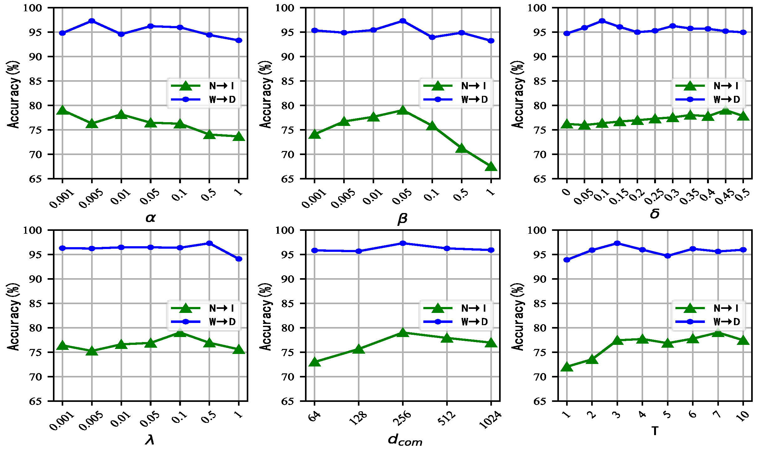
(9) Overall objective function

Based on the above discussion, the overall optimization objective of the CCSMN is to minimize the following loss function:

$$\mathcal{L}=\alpha {\mathcal{L}}_{DCR}+\beta {\mathcal{L}}_{NA}+{\mathcal{L}}_{NS}+\lambda {\mathcal{L}}_{SS}+{\mathcal{L}}_{CLS}^S$$

(17)

where $\alpha$, $\beta$, and $\lambda$ are the corresponding balancing parameters for balancing losses. Algorithm 1 summarizes the proposed CCSMN algorithm.

Algorithm 1. CCSMN

Input: Source domain: ${\mathcal{D}}_s=\left\{{\mathcal{X}}_S, {\mathcal{Y}}_S\right\}={\left\{\left(x_s^i,y_s^i\right)\right\}}_{i=1}^{n_s}$; target domain:${\mathcal{D}}_T={\mathcal{D}}_{TL}\cup {\mathcal{D}}_{TU}=\left\{{\mathcal{X}}_L, {\mathcal{Y}}_L\right\}\cup \left\{{\mathcal{X}}_U\right\}={\left\{\left(x_l^i,y_l^i\right)\right\}}_{i=1}^{n_l}\cup {\left\{\left(x_u^i\right)\right\}}_{i=1}^{n_u}$; hyperparameters: $\alpha ,\beta ,\delta ,\lambda and$ T; iteration: N; Common subspace dimension:$d_{com}$

Output: Feature encoders ${\mathsf{\Omega }}_S\left(x_s^i\right),{\mathsf{\Omega }}_T\left(x_t^i\right)$ and Classifier F(··) 1: Initialize the source and target feature encoders: ${\mathsf{\Omega }}_S\left(x_s^i\right), {\mathsf{\Omega }}_T\left(x_t^i\right)$ and Classifier F(··). 2:    for $i=1$ to N do 3:       Get embedded features in common subspaces and network outputs. 4:       Compute normalized embedded features by (3). 5:      The domain centers of the two domains are calculated by (4), and by (5) the global Angle difference of the connected structure of the center of mass is avoided. 6:      Only the pseudo-label predicted by the neural network is consistent with formula (15), the pseudo-label is assigned to an unlabeled target domain sample, and this sample is allowed to participate in model training. 7:       Compute the nodes of two domains by (6) and further strengthen the alignment of nodes between the cross-domains by (7). 8:       Ensure a high degree of similarity in the shape of the two centroid-connected structures by (11) and (13). 9:      Update the network by minimizing losses (17). 10: end for 11: Return the optimal model feature encoder ${\mathsf{\Omega }}_S\left(x_s^i\right), {\mathsf{\Omega }}_T\left(x_t^i\right)$ and classifier F(·).

(10) Time complexity

The time complexity of the proposed method mainly depends on the embedded feature extraction and the pseudo-label prediction of two domain datasets. Assuming there are n samples in the datasets, using a three-layer neural network for label classification prediction, the mapping time complexity is $\mathrm{O}\left({\mathrm{n}}^2\right)$ and the time complexity of three-layer neural network classification is O (m*n), where m is the number of neurons. In the process of calculating class centroid similarity, the time complexity is $\mathrm{O}\left(\mathrm{nlogn}\right)$. Therefore, it can be seen that the time complexity of the method proposed is $\mathrm{O}\left({\mathrm{n}}^2\right)$. The spatial complexity is $\mathrm{O}\left(\mathrm{md}\right)$, where d is the feature dimension.

4. Experiments and Discussion

4.1. Description of Data

In this paper, different transfer tasks are constructed on widely used standard datasets to evaluate the proposed CCSMN. The datasets are shown in

Table 2. Datasets description.

Datasets	Type	Features	Dimensions	Samples	Classes
NUS-WIDE (N)	Text	NN	64	800	8
ImageNet (I)	Image	${\mathrm{DeCAF}}_6$	4096	824
Amazon (A)	Image	SURF/${\mathrm{DeCAF}}_6$	800/4096	958	10
Caltech (C)				1123
Webcam (W)				295
DSLR (D)				157

.

The text-to-image transfer task uses the NUS-WIDE [45] and ImageNet [7] datasets. The NUS-WIDE dataset is a web image set created by the National University of Singapore Media Search Laboratory, which contains 269,648 images from Flicker and the corresponding labeling information. ImageNet is a large-scale image dataset applied in computer vision, containing 5247 labeled synsets and 3.2 million images. The labeled information of the NUS-WIDE (N) and ImageNet (I) image datasets are used for text-to-image transfer tasks. Eight overlapping categories are selected in the two datasets according to the settings of [34,46,47]. The NUS-WIDE labeling information is preprocessed with five layers of neural networks, and the fourth hidden layer is used as a 64-dimensional feature for the text data. DeCAF6 features of 4096 dimensions are used for image data. In NUS-WIDE, 100 texts per category are selected as labeled source domains. In ImageNet, three images per category are randomly selected as labeled target domains, and the remaining portion of each category is used as unlabeled target domains.

The Office [48] and Caltech-256 [49] datasets are used for the image-to-image transfer task. The Office dataset has 31 categories and contains 4652 images from 3 different domains: Amazon (A), Webcam (W), and DSLR (D). The Caltech-256 dataset has 256 categories and contains 30,607 images. SURF features of 800 dimensions and DeCAF6 features of 4096 dimensions are selected as the feature representation for the transfer task. For the source domain, the entire image data are used. For the target domain, three images per category are randomly assigned as the labeled target domain and the remaining portion as the unlabeled target domain. Due to the sample size limitation, the DSLR dataset is only used as the target domain. To demonstrate the robustness of the proposed model in various HDA tasks, two kinds of transfer tasks are set up: (1) object recognition across feature space: transfer tasks with different feature dimensions from the same data domain, e.g., the $A_{SURF}\to A_{DeCAF}$; (2) object recognition across domains and feature spaces: transfer tasks with samples from different data domains and samples with different feature dimensions, e.g., the $A_{SURF}\to W_{DeCAF}$ transfer task.

4.2. Parameter Settings

The proposed method is implemented based on the Pytorch framework [50]. The network is trained by backpropagation in an end-to-end manner, and all experiments are performed using a stochastic gradient descent optimizer with a momentum of 0.9, a weight decay of 0.001, and a learning rate of 0.1. The feature encoder constructed is a neural network using Leaky ReLU [51] as the activation function. In this paper, all hyperparameters are adjusted within a reasonable range, including $\alpha , \beta , \delta , \lambda , T$, and the typical subspace dimension $d_{com}$, and the plotted results are shown in Figure 3. Figure 3 reports the accuracy of HDA tasks’ w.r.t different parameters ($\alpha , \beta , \lambda$) in range of [0.0001 1]. The value of parameters balance the impact across the statistical distribution alignment. Moreover, the parameter $\mathsf{\delta }$ in the range of [0.0001 0.5] is the equilibrium hyperparameter of the loss funciton. The hyperparameters are set empirically for the text-to-image and image-to-image transfer tasks, and the specific hyperparameter settings are shown in

Table 3. Optimal values of hyperparameters for different datasets.

Dataset	$\mathsf{\alpha }$	$\mathsf{\beta }$	$\mathsf{\delta }$	$\mathsf{\lambda }$	${\mathit{d}}_{\mathit{c}\mathit{o}\mathit{m}}$	$\mathit{T}$
$N\to I$	0.001	0.05	0.45	0.1	256	7
$SURF\to DECA{F}_6$	0.005	0.05	0.1	0.5	256	3
$DECA{F}_6\to SURF$	{0.01,0.5}	{0.001,0.005,0.05}	{0.05,0.3}	{0.05,0.5}	256	3,4,5

.

For all experiments, the maximum number of iterations for training is set to 3000, and the classification accuracy of the unlabeled target domain is used as the evaluation metric; see Equation (18).

$$\mathrm{Accuracy}={\displaystyle \frac{\left|x:x\in {\mathcal{X}}_U\wedge {\widehat{\mathcal{Y}}}_U={\mathcal{Y}}_U\right|}{x:x\in {\mathcal{X}}_U}}$$

(18)

where ${\widehat{\mathcal{Y}}}_U$ and ${\mathcal{Y}}_U$ are the predicted and true labels of the unlabeled target domain, respectively.

To verify the parameter sensitivity of the designed model, $N\to I$, $W\left(SURF\right)\to D\left(DeCAF6\right)$ are randomly selected as representative tasks in text-to-image and image-to-image transfer scenarios. The results show that the models present bell-shaped curves in different transfer scenarios, and all of them have a relatively wide selection range of hyperparameter values and obtain results with competitive advantages. In the $N\to I$ task, the model is insensitive to the parameters $\alpha , \delta , \lambda , T, d_{com}$, and the experimental results do not change by more than 7% when these parameters are changed, and the model is more sensitive to the change in parameter $\beta$, but the results do not change by more than 12% when the value of parameter $\beta$ is changed. In the $W\left(SURF\right)\to D\left(DeCAF6\right)$ task, the model is insensitive to all parameters, and the experimental results do not change by more than 3% with different parameters. Overall, the above experiments demonstrate the robustness of the CCSMN.

4.3. Experimental Results

We used several state-of-the-art HDA methods for the comparison: DAMA [28], LPJT [33], TIT [34], SDA-PPLS [35], CDLS [52], SHFA [53] and MMDT [54]. Support Vector Machine (${\mathrm{SVM}}_t$) was used as a baseline, and the labeled target domain was used to train the ${\mathrm{SVM}}_t$.

(1) The specific classification results can be found in Table 4 for the text-to-image transfer task. Text-to-image is a challenging transfer task, but compared to the baseline methods, the CCSMN obtains an optimal performance. Compared with supervised Support Vector Machine (${\mathrm{SVM}}_t$) methods, most HDA methods perform well, especially the CCSMN, which improves 17.35% over the ${\mathrm{SVM}}_t$. This excellent performance is rare, showing that HDA can promote domain alignment and reduce distributional differences. Compared with the SDA-PPLS method, which has the second-best performance, the CCSMN is also largely better, with an improvement of 8.05%. This excellent performance fully validates the superiority of the CCSMN, indicating that utilizing the pseudo-labeling strategy, alignment between nodes, and mining structural–semantic information in the domain can effectively promote domain self-adaptation.

(2) The specific classification results can be seen in Table 5, Table 6 and Table 7 for the image-to-image transfer task. To study the heterogeneity of the features more comprehensively, the feature representations of $\mathrm{SURF}$/$DeCA{F}_6$ are migrated to the feature representations of $DeCA{F}_6$/ $\mathrm{SURF}$, respectively. The results of the transfer tasks across the feature space show that the CCSMN is better than the baseline method in most of the transfer tasks, achieving the highest average accuracy. It can be found that the classification accuracy of $\mathrm{SURF}\to DeCA{F}_6$ in Table 5 is much better than that of $DeCA{F}_6\to \mathrm{SURF}$ in Table 6, which not only verifies that $DeCA{F}_6$ with in-depth feature representations is more discriminative than hand-crafted $\mathrm{SURF}$, but also illustrates that there is a difference in the transfer of different features from the same domain.

Meanwhile, the transfer task across domains and feature spaces was designed, and the results are shown in Table 7; it can be seen that the CCSMN achieves optimal results in most of the experiments, which suggests that under the joint effect of the same framework mentioned above, the CCSMN learns more relocatable features and the semantic information of geometric structures. In summary, the above experiments fully demonstrate the effectiveness and robustness of the CCSMN in heterogeneous domain adaptation.

Table 4. Heterogeneous domain adaptation text-to-image classification results (%).

Method	$\mathbf{S}\mathbf{V}{\mathbf{M}}_{\mathit{t}}$	DAMA	MMDT	SHFA	CDLS	LPJT	TIT	SDA-PPLS	CCSMN
Results	62.5 ± 1.2	45.3 ± 2.1	48.6 ± 1.3	61.7 ± 1.6	66.3 ± 0.9	65.1 ± 0.3	69.5 ± 0.8	71.8 ± 0.4	79.3 ± 1.0

Table 4. Heterogeneous domain adaptation text-to-image classification results (%).

Method	$\mathbf{S}\mathbf{V}{\mathbf{M}}_{\mathit{t}}$	DAMA	MMDT	SHFA	CDLS	LPJT	TIT	SDA-PPLS	CCSMN
Results	62.5 ± 1.2	45.3 ± 2.1	48.6 ± 1.3	61.7 ± 1.6	66.3 ± 0.9	65.1 ± 0.3	69.5 ± 0.8	71.8 ± 0.4	79.3 ± 1.0

The source domain is NUS-WIDE, and the target domain is ImageNet.

Table 5. HDA classification results across feature space (%).

Dataset	$\mathbf{S}\mathbf{V}{\mathbf{M}}_{\mathit{t}}$	DAMA	MMDT	SHFA	CDLS	LPJT	TIT	SDA-PPLS	CCSMN
C-C	76.8 ± 1.1	73.8 ± 1.2	80.3 ± 1.2	78.2 ± 1.0	81.8 ± 1.1	76.19 ± 1.5	82.26 ± 1.1	86.74 ± 0.9	88.09 ± 0.8
W-W	87.1 ± 1.1	87.2 ± 0.7	87.3 ± 0.8	90.2 ± 1.3	95.2 ± 0.9	90.72 ± 1.2	92.91 ± 1.0	95.71 ± 1.0	96.10 ± 1.1
A-A	86.3 ± 0.5	87.4 ± 0.5	88.6 ± 1.2	89.5 ± 1.5	91.7 ± 0.2	87.71 ± 0.8	88.63 ± 0.4	92.25 ± 0.8	93.60 ± 0.5
Avg.	83.4 ± 0.9	82.8 ± 0.8	85.4 ± 1.0	85.96 ± 1.3	89.56 ± 0.8	85.13 ± 1.1	87.93 ± 0.8	91.56 ± 0.9	92.60 ± 0.8

Table 5. HDA classification results across feature space (%).

Dataset	$\mathbf{S}\mathbf{V}{\mathbf{M}}_{\mathit{t}}$	DAMA	MMDT	SHFA	CDLS	LPJT	TIT	SDA-PPLS	CCSMN
C-C	76.8 ± 1.1	73.8 ± 1.2	80.3 ± 1.2	78.2 ± 1.0	81.8 ± 1.1	76.19 ± 1.5	82.26 ± 1.1	86.74 ± 0.9	88.09 ± 0.8
W-W	87.1 ± 1.1	87.2 ± 0.7	87.3 ± 0.8	90.2 ± 1.3	95.2 ± 0.9	90.72 ± 1.2	92.91 ± 1.0	95.71 ± 1.0	96.10 ± 1.1
A-A	86.3 ± 0.5	87.4 ± 0.5	88.6 ± 1.2	89.5 ± 1.5	91.7 ± 0.2	87.71 ± 0.8	88.63 ± 0.4	92.25 ± 0.8	93.60 ± 0.5
Avg.	83.4 ± 0.9	82.8 ± 0.8	85.4 ± 1.0	85.96 ± 1.3	89.56 ± 0.8	85.13 ± 1.1	87.93 ± 0.8	91.56 ± 0.9	92.60 ± 0.8

The source and target domains are represented by SURF and DeCAF6 features, respectively.

Table 6. Classification results of HDA across feature space (%).

Dataset	$\mathbf{S}\mathbf{V}{\mathbf{M}}_{\mathit{t}}$	DAMA	MMDT	SHFA	CDLS	LPJT	TIT	SDA-PPLS	CCSMN
C-C	29.1 ± 1.5	28.9 ± 1.3	30.6 ± 1.7	29.1 ± 1.5	31.8 ± 1.2	23.01 ± 1.0	32.87 ± 1.1	33.18 ± 0.3	35.50 ± 0.5
W-W	57.9 ± 1.0	58.3 ± 1.4	59.1 ± 1.2	62.2 ± 0.7	63.1 ± 1.1	61.42 ± 1.7	70.66 ± 1.3	71.72 ± 1.1	72.32 ± 1.0
A-A	43.4 ± 0.9	42.4 ± 0.9	40.5 ± 1.3	42.9 ± 1.0	46.4 ± 1.0	36.08 ± 1.3	53.23 ± 1.1	54.88 ± 1.5	53.77 ± 1.4
Avg.	43.46 ± 1.1	43.2 ± 1.2	43.4 ± 1.4	44.73	47.1 ± 1.1	40.17 ± 1.3	52.25 ± 1.1	53.26 ± 0.9	53.86 ± 1.0

Table 6. Classification results of HDA across feature space (%).

Dataset	$\mathbf{S}\mathbf{V}{\mathbf{M}}_{\mathit{t}}$	DAMA	MMDT	SHFA	CDLS	LPJT	TIT	SDA-PPLS	CCSMN
C-C	29.1 ± 1.5	28.9 ± 1.3	30.6 ± 1.7	29.1 ± 1.5	31.8 ± 1.2	23.01 ± 1.0	32.87 ± 1.1	33.18 ± 0.3	35.50 ± 0.5
W-W	57.9 ± 1.0	58.3 ± 1.4	59.1 ± 1.2	62.2 ± 0.7	63.1 ± 1.1	61.42 ± 1.7	70.66 ± 1.3	71.72 ± 1.1	72.32 ± 1.0
A-A	43.4 ± 0.9	42.4 ± 0.9	40.5 ± 1.3	42.9 ± 1.0	46.4 ± 1.0	36.08 ± 1.3	53.23 ± 1.1	54.88 ± 1.5	53.77 ± 1.4
Avg.	43.46 ± 1.1	43.2 ± 1.2	43.4 ± 1.4	44.73	47.1 ± 1.1	40.17 ± 1.3	52.25 ± 1.1	53.26 ± 0.9	53.86 ± 1.0

The source and target domains are represented by DeCAF6 and SURF features, respectively.

Table 7. Classification results of HDA across domains and feature spaces (%).

Dataset	$\mathbf{S}\mathbf{V}{\mathbf{M}}_{\mathit{t}}$	DAMA	MMDT	SHFA	CDLS	LPJT	TIT	SDA-PPLS	CCSMN
A-C	78.5 ± 1.4	78.1 ± 1.5	78.1 ± 1.2	79.5 ± 1.7	83.8 ± 2.3	78.92 ± 1.0	81.31 ± 1.3	85.49 ± 0.8	88.10 ± 0.6
A-W	88.7 ± 2.1	89.4 ± 1.5	89.4 ± 1.5	90.1 ± 0.8	93.6 ± 1.5	90.79 ± 1.5	91.87 ± 0.8	93.94 ± 1.5	93.55 ± 1.4
A-D	90.9 ± 1.2	91.5 ± 1.2	92.1 ± 1.1	93.4 ± 1.5	96.1 ± 0.7	90.39 ± 1.2	94.29 ± 1.2	94.88 ± 1.0	96.76 ± 1.3
C-A	86.9 ± 1.9	87.5 ± 1.1	87.5 ± 1.1	88.6 ± 1.1	90.7 ± 1.9	88.99 ± 1.3	89.47 ± 1.3	91.36 ± 1.7	93.15 ± 0.5
C-W	88.7 ± 2.1	88.9 ± 1.6	88.9 ± 1.3	89.6 ± 1.6	92.5 ± 1.3	89.83 ± 1.2	91.47 ± 1.0	94.62 ± 1.5	93.77 ± 1.3
C-D	90.9 ± 1.2	91.0 ± 1.3	93.1 ± 1.1	93.8 ± 1.2	94.9 ± 1.5	91.1 ± 1.3	95.31 ± 0.9	94.96 ± 1.4	96.15 ± 1.5
W-C	78.5 ± 1.4	78.6 ± 1.2	78.6 ± 1.7	79.7 ± 1.2	82.1 ± 1.2	78.6 ± 1.1	80.42 ± 1.6	85.4 ± 0.6	87.40 ± 0.8
W-A	86.9 ± 1.9	88.3 ± 1.4	88.3 ± 1.4	88.7 ± 1.5	90.5 ± 1.3	90.36 ± 1.4	89.19 ± 1.4	90.97 ± 1.3	92.62 ± 1.0
W-D	90.9 ± 1.7	91.2 ± 0.9	91.5 ± 1.3	92.4 ± 1.0	95.1 ± 0.8	90.2 ± 1.9	94.53 ± 1.1	96.84 ± 1.1	97.30 ± 1.2
Avg.	86.76 ± 1.7	87.1 ± 1.3	87.5 ± 1.4	88.42 ± 1.3	91.03 ± 1.4	87.68 ± 1.3	89.76 ± 1.1	92.05 ± 1.2	93.20 ± 1.1

Table 7. Classification results of HDA across domains and feature spaces (%).

Dataset	$\mathbf{S}\mathbf{V}{\mathbf{M}}_{\mathit{t}}$	DAMA	MMDT	SHFA	CDLS	LPJT	TIT	SDA-PPLS	CCSMN
A-C	78.5 ± 1.4	78.1 ± 1.5	78.1 ± 1.2	79.5 ± 1.7	83.8 ± 2.3	78.92 ± 1.0	81.31 ± 1.3	85.49 ± 0.8	88.10 ± 0.6
A-W	88.7 ± 2.1	89.4 ± 1.5	89.4 ± 1.5	90.1 ± 0.8	93.6 ± 1.5	90.79 ± 1.5	91.87 ± 0.8	93.94 ± 1.5	93.55 ± 1.4
A-D	90.9 ± 1.2	91.5 ± 1.2	92.1 ± 1.1	93.4 ± 1.5	96.1 ± 0.7	90.39 ± 1.2	94.29 ± 1.2	94.88 ± 1.0	96.76 ± 1.3
C-A	86.9 ± 1.9	87.5 ± 1.1	87.5 ± 1.1	88.6 ± 1.1	90.7 ± 1.9	88.99 ± 1.3	89.47 ± 1.3	91.36 ± 1.7	93.15 ± 0.5
C-W	88.7 ± 2.1	88.9 ± 1.6	88.9 ± 1.3	89.6 ± 1.6	92.5 ± 1.3	89.83 ± 1.2	91.47 ± 1.0	94.62 ± 1.5	93.77 ± 1.3
C-D	90.9 ± 1.2	91.0 ± 1.3	93.1 ± 1.1	93.8 ± 1.2	94.9 ± 1.5	91.1 ± 1.3	95.31 ± 0.9	94.96 ± 1.4	96.15 ± 1.5
W-C	78.5 ± 1.4	78.6 ± 1.2	78.6 ± 1.7	79.7 ± 1.2	82.1 ± 1.2	78.6 ± 1.1	80.42 ± 1.6	85.4 ± 0.6	87.40 ± 0.8
W-A	86.9 ± 1.9	88.3 ± 1.4	88.3 ± 1.4	88.7 ± 1.5	90.5 ± 1.3	90.36 ± 1.4	89.19 ± 1.4	90.97 ± 1.3	92.62 ± 1.0
W-D	90.9 ± 1.7	91.2 ± 0.9	91.5 ± 1.3	92.4 ± 1.0	95.1 ± 0.8	90.2 ± 1.9	94.53 ± 1.1	96.84 ± 1.1	97.30 ± 1.2
Avg.	86.76 ± 1.7	87.1 ± 1.3	87.5 ± 1.4	88.42 ± 1.3	91.03 ± 1.4	87.68 ± 1.3	89.76 ± 1.1	92.05 ± 1.2	93.20 ± 1.1

4.4. Experimental Analysis

4.4.1. Ablation Studies

The ablation study focuses on empirically evaluating several variants of the model:

• The model ($\alpha =0$) eliminates the domain-centered rotation mechanism;
• The model ($\beta =0$) eliminates the node attraction mechanism;
• The model ($\delta =0$) eliminates the node semantic sharing mechanism;
• The model ($\lambda =0$) eliminates the structure semantic sharing mechanism.

In

Table 8. CCSMN ablation studies.

Method	$\mathit{N}\to \mathbf{I}$	$\mathbf{W}\to \mathbf{W}$	$\mathbf{C}\to \mathbf{A}$
$\mathrm{CCSMN} \left(\alpha =0\right)$	78.36 ± 1.7	95.42 ± 1.0	92.37 ± 0.9
$\mathrm{CCSMN} \left(\beta =0\right)$	75.54 ± 1.8	95.41 ± 0.7	92.24 ± 0.9
$\mathrm{CCSMN} \left(\mathsf{\delta }=0\right)$	78.02 ± 1.8	95.26 ± 1.9	92.96 ± 0.5
$\mathrm{CCSMN} \left(\lambda =0\right)$	77.61 ± 1.7	95.23 ± 1.6	93.05 ± 0.8
$\mathrm{CCSMN} \left(\mathrm{full}\right)$	79.27 ± 1.0	96.10 ± 1.1	93.15 ± 0.5

, three transfer tasks were randomly selected for ablation experiments to investigate the effects of different components in the CCSMN. The results in Table 8 show that the elimination of each of the four variables of the CCSMN has a specific effect. Still, the performance is significantly reduced, and none of them is as good as the CCSMN(full), which suggests that all the components are essential and integral to facilitating a positive transfer. The necessity of alignment and semantic sharing between nodes for the migration task from the whole model perspective reflects the proposed CCSMN’s effectiveness.

4.4.2. Feature Visualization

To analyze the adaptive capability of the proposed CCSMN model, this paper takes $W\left(SURF\right)\to C\left(DeCAF6\right)$ as an example, and adopts the t-SNE [55] technique to visualize the feature distribution of the public subspace before and after the domain adaptation in Figure 4. Different colors indicate different categories, where “squares” indicate all source domain samples and “circles” indicate all target domain samples. As can be seen in Figure 4a, there is no domain adaptation between these two domains, i.e., only the neural network is used for predictive classification, and the result shows a highly mixed feature distribution, where it is difficult to distinguish the categories they belong to. There is more overlap between different categories. In contrast, as shown in Figure 4b, our CCSMN can show more compact clusters for different categories, and the boundaries between the clusters are more prominent, with only very few mislabels. Overall, the CCSMN can achieve better intra-class compactness and inter-class separability, indicating the superior performance of the CCSMN in learning domain-invariant and discriminative feature representations.

5. Conclusions and Future Work

The paper proposes a centroid-connected structure matching network (CCSMN) to solve the HDA problem in end-to-end deep neural networks. The CCSMN focuses on learning adaptive classifiers and domain-invariant and discriminative feature subspaces. Compared with existing HDA methods, the CCSMN transforms the data into features of the same dimension in a shared feature subspace, and some mechanisms that enhance the intrinsic structure of semantic information are used to improve transfer similarity. During training, the pseudo-label co-decision mechanism assigns pseudo-labels to the target domain. Ultimately, high-performing classifiers and discriminative, domain-invariant subspace networks are obtained. The superiority of the CCSMN over some state-of-the-art HDA methods is verified under extensive experiments. The method proposed is still a shallow approach, and the experimental data must have clear label and category information, and it may not effectively handle open domain datasets and multimodal data such as videos. Future work should extend the proposed method to open-set HDA scenarios, multi-modal source domains, and deep learning frameworks.