Testing Spherical Symmetry Based on Statistical Representative Points

Abstract

This paper introduces a novel chisquare test for spherical symmetry, utilizing statistical representative points. The proposed representative-point-based chisquare statistic is shown, through a Monte Carlo study, to considerably improve the power performance compared to the traditional equiprobable chisquare test in many high-dimensional cases. While the test requires relatively large sample sizes to approximate the chisquare distribution, obtaining critical values from existing chisquare tables is simpler compared to many existing tests for spherical symmetry. A real-data application demonstrates the robustness of the proposed method against different choices of representative points. This paper argues that the use of representative points provides a new perspective in high-dimensional goodness-of-fit testing, offering an alternative approach to evaluating spherical symmetry in such contexts. By leveraging the flexibility of choosing the number of representative points, this method ensures more reliable detection of departures from spherical symmetry, especially in high-dimensional datasets. Overall, this research highlights the practical advantages of the proposed approach in statistical analysis, emphasizing its potential as a powerful tool in goodness-of-fit tests within the realm of high-dimensional data.

1. Introduction

Spherical distributions are extensions of the multivariate standard normal distribution. The theory of spherical distributions plays an important role in constructing new types of statistics for statistical inference [1,2,3,4,5,6,7,8,9,10,11,12]. Some good properties of the new type of statistics constructed by the theory of spherical distributions are discussed and illustrated by both Monte Carlo studies and real-life examples in these references. Spherical distributions have been applied to the extension of the regular normal errors in regression models by researchers to characterize the fat-tailed distributional properties for some practical situations [13,14,15,16,17,18,19,20,21].

Similar to the extensions of the multivariate standard normal distribution to the general multivariate normal distribution, spherical distributions are naturally extended to the family of elliptically contoured distributions (ECDs, for simplicity) through linear transformation [2,21]. The problem of testing the goodness of fit for ECDs is closely related to testing spherical symmetry [22,23], which has been studied for around half a century, see, for example, [24,25,26,27,28,29,30,31,32,33]. Therefore, it is essential to develop goodness-of-fit tests for spherical symmetry first and then a linear transformation can be applied to the original i.i.d. (independent identically distributed) sample.

In this paper, we will apply the idea of statistical representative points (RPs, [34]) or the so-called principal points [35] to the construction of the classical Pearson–Fisher chisquare test for the general purpose of goodness of fit. The RP idea for constructing and improving goodness-of-fit tests for multivariate normality has been proved effective, as demonstrated by the papers [36,37]. The same RP idea can be applied to constructing goodness-of-fit tests for high-dimensional spherical symmetry. A simple Monte Carlo study was conducted to assess the performance of the new method compared with the traditional equiprobable construction of the classical Pearson–Fisher chisquare test. The results indicate that the new statistics exhibit good control over type I error rates across a range of settings, ensuring that the tests do not reject the null hypothesis of spherical symmetry too often when it is true. Moreover, the power of the proposed test, i.e., the ability to detect departures from spherical symmetry, was found to be competitive, often surpassing that of the existing equiprobable chisquare test, particularly in high-dimensional contexts where traditional methods tend to struggle. The core strength of our approach lies in its ability to adapt to different sample sizes and dimensionalities without compromising statistical power. This flexibility makes it particularly useful for modern applications involving high-dimensional complex data structures. Section 2 gives the basic idea for constructing the RP chisquare test and equiprobable chisquare. Section 3 presents a Monte Carlo comparison between the two construction methods of the Pearson–Fisher chisquare test and a simple comparison between the proposed chisquare approach and two existing ones in two low-dimensional cases. The proposed methods are illustrated by a real-data example in Section 3.4. Some concluding remarks and a simple discussion are given in Section 4.

2. The Construction of the RP Chisquare and the Equiprobable Chisquare Tests

The traditional Pearson–Fisher chisquare test for the general purpose of goodness of fit is to test if a set of i.i.d. samples $\{X_1,\dots ,X_n\}$ can be considered from a population with a known probability distribution function $F\left(x\right)$ defined by

$$H_0:\{X_1,\dots ,X_n\}\mathrm{is} \mathrm{a} \mathrm{sample} \mathrm{from}F\left(x\right)$$

(1)

against the general alternative that $H_1$: $H_0$ is not true. Let

$$-\infty =a_0<a_1<\dots <a_{m-1}<a_m=+\infty .$$

(2)

be a set of interval endpoints and

$$\begin{array}{ccc}{\displaystyle n_i}\hfill & =& \mathrm{the} \mathrm{number} \mathrm{of} \mathrm{observed} \mathrm{sample} \mathrm{points} \mathrm{located} \mathrm{in} \mathrm{the} \mathrm{interval}\hfill \\ I_i\hfill & =& {\displaystyle (a_{i-1},a_i),i=1,\dots ,m.}\hfill \end{array}$$

(3)

The traditional PF chisquare test for hypothesis (1) is defined by

$${\chi }_T^2=\sum _{i=1}^m{\displaystyle \frac{{(n_i-n{p}_i)}^2}{n{p}_i}},$$

(4)

where

$$p_i={\int }_{a_{i-1}}^{a_i}dF\left(x\right),i=1,\dots ,m$$

(5)

is the cell probability. It is known that under the null hypothesis (1), the PF chisquare statistic in (4) has an asymptotic chisquare distribution ${\chi }^2(m-1)$. The idea for equiprobable chisquare is to choose the interval points in (2) so that the cell probabilities $p_i$ in (5) are the same: $p_i\equiv 1/m$. Voinov et al. [38] studied various choices for the cell classification in constructing the general chisquare test and pointed out some competitiveness of the equiprobable choice when there is no prior information.

The early idea of defining and finding statistical representative points (RPs) can be referred to [33,35]. The RP idea for constructing multivariate goodness-of-fit tests can be referred to [36,37]. Let $\{R_1,\dots ,R_m\}$ be a set of RPs from the given probability distribution in hypothesis (1). Define the cell intervals

$$\begin{array}{ccc}\hfill {\displaystyle J_1}& =& {\displaystyle \left(-\infty ,\frac{R_1+R_2}{2}\right),J_2=\left[\frac{R_1+R_2}{2},\frac{R_2+R_3}{2}\right),\dots ,}\hfill \\ \hfill {\displaystyle J_{m-1}}& =& {\displaystyle \left[\frac{R_{m-2}+R_{m-1}}{2},\frac{R_{m-1}+R_m}{2}\right),J_m=\left[\frac{R_{m-1}+R_m}{2},+\infty \right)}\hfill \end{array}$$

(6)

and the probabilities

$$q_i={\int }_{J_i}dF\left(x\right),i=1,\dots ,m,$$

(7)

The RP chisquare for testing hypothesis (1) is computed by

$${\chi }_R^2=\sum _{i=1}^m{\displaystyle \frac{{(f_i-n{q}_i)}^2}{n{q}_i}}\to {\chi }^2(m-1),$$

(8)

under the null hypothesis (1), where $f_i$ is the number of sample points located in the interval $J_i$.

In this paper, we want to test whether a set of i.i.d. d-dimensional ($d\ge 2$) random sample $\{x_1,\dots ,x_n\}$ can be considered to come from a population with a d-dimensional spherical distribution, denoted by ${\mathcal{S}}_d\left(\varphi \right)$, with $\varphi (·)$ being the characteristic function. The hypothesis can be expressed as

$$H_0:\{x_1,\dots ,x_n\}\sim {\mathcal{S}}_d\left(\varphi \right)\mathrm{for} \mathrm{some} \mathrm{scalar} \mathrm{function}\varphi (·)$$

(9)

against the general alternative hypothesis $H_1$: $\{x_1,\dots ,x_n\}\notin {\mathcal{S}}_p\left(\varphi \right)$. Hypothesis (9) belongs to an entry in “Testing Spherical and Elliptical Symmetry” in the Encyclopedia of Statistics [39], which includes most of the currently published research papers in this direction. It still remains an everlasting interest among statisticians even after almost twenty years have passed. Simply speaking, the characteristic of a spherical distribution is its rotational invariance, like

$$\mathit{x}\stackrel{\mathrm{d}}{=}\mathbf{\Gamma }x,$$

(10)

where $\mathbf{\Gamma }$ is a $d\times d$ constant orthogonal matrix such that ${\mathbf{\Gamma }}^{\prime }\mathbf{\Gamma }=\mathbf{\Gamma }{\mathbf{\Gamma }}^{\prime }={\mathit{I}}_d$ and the sign “$\stackrel{\mathrm{d}}{=}$” means that both sides of the equation have the same distribution. We denote $\mathit{x}\sim {\mathcal{S}}_d\left(\varphi \right)$ if x satisfies (10). If $\mathit{x}\sim {\mathcal{S}}_d\left(\varphi \right)$, then the characteristic function (c.f.) of x has the form $\varphi \left({\mathit{t}}^{\prime }\mathit{t}\right)={\varphi (\parallel \mathit{t}\parallel }^2)$ ($\mathit{t}\in R^d$; the d-dimensional Euclidean space, $\parallel ·\parallel$ stands for the Euclidean norm). The following basic lemma is from [1], which gives a simple characterization of spherical distributions.

Lemma 1. 

(Theorem 2.22 of [1], p. 51) Let z be a random vector in $R^d$ with $P(\mathit{z}=\mathbf{0})=0$. The distribution of a statistic $t\left(\mathit{z}\right)$ remains unchanged if $\mathit{z}\sim S_d\left(\varphi \right)$ and

$$t\left(a\mathit{z}\right)\stackrel{\mathrm{d}}{=}t\left(\mathit{z}\right),\mathit{for} \mathit{any} \mathit{constant} a>0.$$

(11)

In particular,

$$t\left(\mathit{z}\right)\stackrel{\mathrm{d}}{=}t\left({\mathit{z}}_0\right),for any z\sim S_d\left(\varphi \right)with P(\mathit{z}=\mathbf{0})=0,$$

(12)

where ${\mathit{z}}_0\sim N_d(\mathbf{0},{\mathit{I}}_d)$, which stands for the d-dimensional standard normal distribution.

Let us denote $\mathit{z}\sim S_d\left(\varphi \right)$ with $P(\mathit{z}=\mathbf{0})=0$ as $\mathit{z}\sim S_d^{+}\left(\varphi \right)$. Based on Lemma 1, if we have an i.i.d. sample ${\mathit{x}}_1,\dots ,{\mathit{x}}_n$ from $S_d^{+}\left(\varphi \right)$, and $x_i={(x_{i1},\dots ,x_{id})}^{\prime }$ ($i=1,\dots ,n$), we can define

$$T_i={\displaystyle \frac{\sqrt{d}{\overline{x}}_i}{s_i}},{\overline{x}}_i={\displaystyle \frac{1}{d}}\sum _{j=1}^d{x}_{ij},s_i^2={\displaystyle \frac{1}{d-1}}\sum _{j=1}^d{(x_{ij}-{\overline{x}}_i)}^2,$$

(13)

Then, $\{T_i:i=1,\dots ,n\}$ is an i.i.d. sample from the Student’s t-distribution $t(d-1)$, because each $T_i$ is scale-invariant. It is obvious that there are many scale-invariant statistics satisfying (11) and (12). Li et al. [6] constructed a t-plot, F-plot, and $\beta$-plot for detecting the non-spherical symmetry of multivariate samples. They proposed to use the correlation coefficient as a statistic for a double-check of analytical tests for evaluating the linearity of the three plots. Here, we propose to use the idea of statistical representative points to construct a general chisquare test for goodness of fit. There are certainly other tests available for the same purpose, such as the Kolmorov–Smirnov (KS) statistic and the Anderson–Darling statistic (AD) [40]. Based on this conclusion, we can transfer a test for spherical symmetry (9) to a test for Student’s t-distribution $t(d-1)$:

$$\begin{array}{cc}& {\displaystyle H_0:\{T_i:i=1,\dots ,n\}\sim t(d-1)}\hfill \\ \hfill \mathrm{versus}& {\displaystyle H_1:\{T_i:i=1,\dots ,n\}\mathrm{is} \mathrm{not} \mathrm{from}t(d-1).}\hfill \end{array}$$

(14)

A test for (14) is called a necessary one for (9) [27], which means that rejection of (14) results in rejection of (9) at the same level of significance. But non-rejection of (14) generally does not result in the truth of (9). The representative points and their associated interval probabilities in the intervals (6) and (7) for some univariate continuous distributions can be obtained directly from the website https://fst.uic.edu.cn/isci_en/Representative_Points/Representative_Points_for_Different_Statistical_Di.htm (accessed on 8 December 2024). Therefore, the RP chisquare statistic in (8) for testing (14) can be easily computed. We present a simple Monte Carlo study in the next section.

3. An Empirical Comparison Between the RP Chisquare and the Equiprobable Chisquare Tests

3.1. Empirical Type I Error Rates

There are many spherically symmetric distributions (SSDs, for simplicity). Fang et al. [1] gave a thorough discussion on some subfamilies of SSDs. We choose the following ones for our Monte Carlo study on a simple empirical type I error comparison between the RP chisquare and the equiprobable chisquare tests in the aspect of controlling type I error rates. These SSDs are as follows:

(1)

The standard normal distribution $N_d(\mathbf{0},{\mathit{I}}_d)$;

(2)

The multivariate t-distribution $t\left(10\right)$, with degrees of freedom $df=10$;

(3)

The Kotz-type distribution with parameters $N=5$, $r=1$, and $s=1$.

The so-called TFWW algorithm ([41]; [42], pp. 166–170) is employed to generate empirical samples from the selected non-normal spherical distributions. The normal samples are generated by a MATLAB (R216b) internal function.

Table 1. Empirical type I error rates with t-representative points for multivariate normal distribution $N_d(\mathbf{0},{\mathit{I}}_d$) ($\alpha =0.05$).

n	m	${\mathit{\chi }}^2$	$\mathit{d}=5$	$\mathit{d}=10$	$\mathit{d}=15$	$\mathit{d}=20$	$\mathit{d}=25$
$n=50$	$m=5$	${\chi }_R^2$	0.0130	0.0115	0.0095	0.0115	0.0135
		${\chi }_T^2$	0.0165	0.0135	0.0090	0.0080	0.0170
	$m=10$	${\chi }_R^2$	0.0410	0.0200	0.0165	0.0155	0.0210
		${\chi }_T^2$	0.0235	0.0165	0.0240	0.0170	0.0205
	$m=15$	${\chi }_R^2$	0.0600	0.0365	0.0290	0.0310	0.0230
		${\chi }_T^2$	0.0315	0.0205	0.0255	0.0275	0.0235
	$m=20$	${\chi }_R^2$	0.0830	0.0505	0.0325	0.0335	0.0325
		${\chi }_T^2$	0.0265	0.0265	0.0230	0.0285	0.0205
$n=100$	$m=5$	${\chi }_R^2$	0.0085	0.0115	0.0070	0.0135	0.0115
		${\chi }_T^2$	0.0130	0.0160	0.0100	0.0130	0.0170
	$m=10$	${\chi }_R^2$	0.0465	0.0200	0.0230	0.0180	0.0165
		${\chi }_T^2$	0.0225	0.0190	0.0235	0.0215	0.0245
	$m=15$	${\chi }_R^2$	0.0830	0.0310	0.0250	0.0230	0.0200
		${\chi }_T^2$	0.0245	0.0235	0.0205	0.0250	0.0240
	$m=20$	${\chi }_R^2$	0.0550	0.0320	0.0295	0.0275	0.0230
		${\chi }_T^2$	0.0335	0.0245	0.0230	0.0190	0.0275
$n=200$	$m=5$	${\chi }_R^2$	0.0120	0.0135	0.0130	0.0125	0.0110
		${\chi }_T^2$	0.0135	0.0145	0.0115	0.0145	0.0210
	$m=10$	${\chi }_R^2$	0.0250	0.0190	0.0200	0.0210	0.0215
		${\chi }_T^2$	0.0180	0.0190	0.0200	0.0185	0.0225
	$m=15$	${\chi }_R^2$	0.0740	0.0345	0.0235	0.0210	0.0205
		${\chi }_T^2$	0.0225	0.0285	0.0225	0.0260	0.0235
	$m=20$	${\chi }_R^2$	0.0595	0.0325	0.0320	0.0240	0.0325
		${\chi }_T^2$	0.0255	0.0255	0.0420	0.0260	0.0275
$n=400$	$m=5$	${\chi }_R^2$	0.0140	0.0085	0.0100	0.0110	0.0120
		${\chi }_T^2$	0.0200	0.0090	0.0125	0.0115	0.0120
	$m=10$	${\chi }_R^2$	0.0255	0.0245	0.0185	0.0250	0.0190
		${\chi }_T^2$	0.0205	0.0225	0.0200	0.0195	0.0170
	$m=15$	${\chi }_R^2$	0.0400	0.0250	0.0285	0.0265	0.0265
		${\chi }_T^2$	0.0270	0.0245	0.0205	0.0260	0.0225
	$m=20$	${\chi }_R^2$	0.0760	0.0240	0.0265	0.0290	0.0250
		${\chi }_T^2$	0.0235	0.0240	0.0250	0.0325	0.0255

,

Table 2. Empirical type I error rates with t-representative points for multivariate t distribution with $df=10$ ($\alpha =0.05$).

n	m	${\mathit{\chi }}^2$	$\mathit{d}=5$	$\mathit{d}=10$	$\mathit{d}=15$	$\mathit{d}=20$	$\mathit{d}=25$
$n=50$	$m=5$	${\chi }_R^2$	0.0160	0.0135	0.0095	0.0105	0.0125
		${\chi }_T^2$	0.0110	0.0115	0.0130	0.0135	0.0105
	$m=10$	${\chi }_R^2$	0.0465	0.0210	0.0205	0.0140	0.0185
		${\chi }_T^2$	0.0225	0.0220	0.0155	0.0135	0.0170
	$m=15$	${\chi }_R^2$	0.0570	0.0330	0.0350	0.0180	0.0220
		${\chi }_T^2$	0.0250	0.0265	0.0285	0.0245	0.0265
	$m=20$	${\chi }_R^2$	0.0945	0.0600	0.0340	0.0295	0.0235
		${\chi }_T^2$	0.0230	0.0250	0.0280	0.0295	0.0245
$n=100$	$m=5$	${\chi }_R^2$	0.0135	0.0140	0.0155	0.0180	0.0150
		${\chi }_T^2$	0.0165	0.0205	0.0165	0.0145	0.0160
	$m=10$	${\chi }_R^2$	0.0530	0.0255	0.0215	0.0240	0.0205
		${\chi }_T^2$	0.0215	0.0195	0.0235	0.0215	0.0205
	$m=15$	${\chi }_R^2$	0.0750	0.0340	0.0335	0.0230	0.0265
		${\chi }_T^2$	0.0285	0.0275	0.0205	0.0300	0.0240
	$m=20$	${\chi }_R^2$	0.0570	0.0405	0.0335	0.0370	0.0285
		${\chi }_T^2$	0.0325	0.0270	0.0235	0.0330	0.0365
$n=200$	$m=5$	${\chi }_R^2$	0.0155	0.0110	0.0090	0.0130	0.0075
		${\chi }_T^2$	0.0120	0.0165	0.0160	0.0120	0.0100
	$m=10$	${\chi }_R^2$	0.0295	0.0220	0.0210	0.0245	0.0165
		${\chi }_T^2$	0.0220	0.0210	0.0235	0.0330	0.0190
	$m=15$	${\chi }_R^2$	0.0885	0.0320	0.0300	0.0245	0.0220
		${\chi }_T^2$	0.0285	0.0245	0.0220	0.0320	0.0215
	$m=20$	${\chi }_R^2$	0.0630	0.0395	0.0425	0.0280	0.0250
		${\chi }_T^2$	0.0305	0.0285	0.0290	0.0315	0.0325
$n=400$	$m=5$	${\chi }_R^2$	0.0135	0.0130	0.0125	0.0115	0.0160
		${\chi }_T^2$	0.0145	0.0165	0.0140	0.0115	0.0155
	$m=10$	${\chi }_R^2$	0.0285	0.0200	0.0190	0.0265	0.0185
		${\chi }_T^2$	0.0195	0.0230	0.0255	0.0175	0.0265
	$m=15$	${\chi }_R^2$	0.0485	0.0295	0.0385	0.0285	0.0265
		${\chi }_T^2$	0.0260	0.0220	0.0235	0.0255	0.0270
	$m=20$	${\chi }_R^2$	0.0770	0.0340	0.0400	0.0300	0.0310
		${\chi }_T^2$	0.0325	0.0310	0.0245	0.0305	0.0255

and

Table 3. Empirical type I error rates with t-representative points for multivariate Kotz-type distribution $M{K}_d(5,1,1)$ ($\alpha =0.05$).

n	m	${\mathit{\chi }}^2$	$\mathit{d}=5$	$\mathit{d}=10$	$\mathit{d}=15$	$\mathit{d}=20$	$\mathit{d}=25$
$n=50$	$m=5$	${\chi }_R^2$	0.0160	0.0120	0.0105	0.0130	0.0080
		${\chi }_T^2$	0.0105	0.0130	0.0145	0.0115	0.0155
	$m=10$	${\chi }_R^2$	0.0330	0.0175	0.0205	0.0235	0.0150
		${\chi }_T^2$	0.0205	0.0130	0.0230	0.0220	0.0210
	$m=15$	${\chi }_R^2$	0.0520	0.0370	0.0310	0.0210	0.0275
		${\chi }_T^2$	0.0220	0.0325	0.0230	0.0215	0.0250
	$m=20$	${\chi }_R^2$	0.0765	0.0535	0.0440	0.0265	0.0330
		${\chi }_T^2$	0.0220	0.0250	0.0265	0.0260	0.0245
$n=100$	$m=5$	${\chi }_R^2$	0.0080	0.0090	0.0125	0.0080	0.0120
		${\chi }_T^2$	0.0105	0.0140	0.0155	0.0180	0.0150
	$m=10$	${\chi }_R^2$	0.0390	0.0220	0.0240	0.0145	0.0195
		${\chi }_T^2$	0.0165	0.0185	0.0195	0.0220	0.0210
	$m=15$	${\chi }_R^2$	0.0800	0.0275	0.0335	0.0255	0.0285
		${\chi }_T^2$	0.0155	0.0275	0.0215	0.0215	0.0245
	$m=20$	${\chi }_R^2$	0.0525	0.0365	0.0445	0.0385	0.0235
		${\chi }_T^2$	0.0250	0.0205	0.0225	0.0255	0.0260
$n=200$	$m=5$	${\chi }_R^2$	0.0115	0.0125	0.0120	0.0110	0.0095
		${\chi }_T^2$	0.0115	0.0125	0.0180	0.0130	0.0135
	$m=10$	${\chi }_R^2$	0.0285	0.0225	0.0230	0.0130	0.0260
		${\chi }_T^2$	0.0200	0.0220	0.0190	0.0145	0.0175
	$m=15$	${\chi }_R^2$	0.0765	0.0315	0.0300	0.0255	0.0270
		${\chi }_T^2$	0.0275	0.0250	0.0275	0.0265	0.0245
	$m=20$	${\chi }_R^2$	0.0665	0.0375	0.0365	0.0285	0.0210
		${\chi }_T^2$	0.0320	0.0335	0.0245	0.0325	0.0270
$n=400$	$m=5$	${\chi }_R^2$	0.0130	0.0065	0.0110	0.0160	0.0095
		${\chi }_T^2$	0.0125	0.0120	0.0115	0.0075	0.0155
	$m=10$	${\chi }_R^2$	0.0195	0.0205	0.0195	0.0195	0.0200
		${\chi }_T^2$	0.0210	0.0215	0.0185	0.0235	0.0235
	$m=15$	${\chi }_R^2$	0.0375	0.0240	0.0295	0.0205	0.0270
		${\chi }_T^2$	0.0300	0.0230	0.0185	0.0245	0.0280
	$m=20$	${\chi }_R^2$	0.0775	0.0300	0.0405	0.0255	0.0265
		${\chi }_T^2$	0.0270	0.0260	0.0310	0.0265	0.0285

summarize the simulation results based on 2000 simulation replications with size $\alpha =0.05$. Results for $\alpha =0.01$ and $\alpha =0.10$ are also available upon request. We only present the case of $\alpha =0.05$ to save space. The simulation results in Table 1, Table 2 and Table 3 demonstrate that both the traditional equiprobable chisquare and the RP chisquare seem to underestimate the type I error rates under different sample sizes and numbers of RPs.

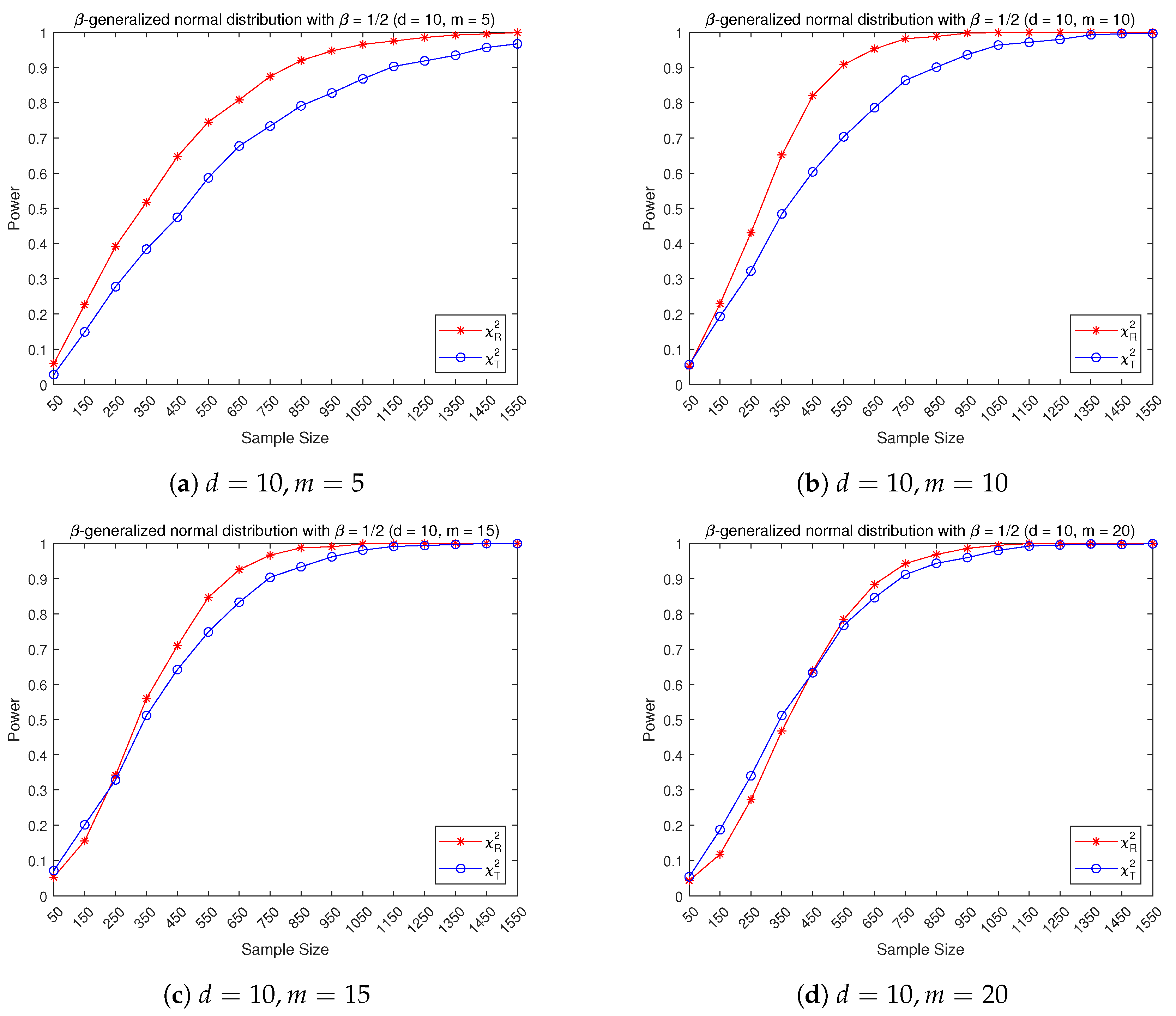
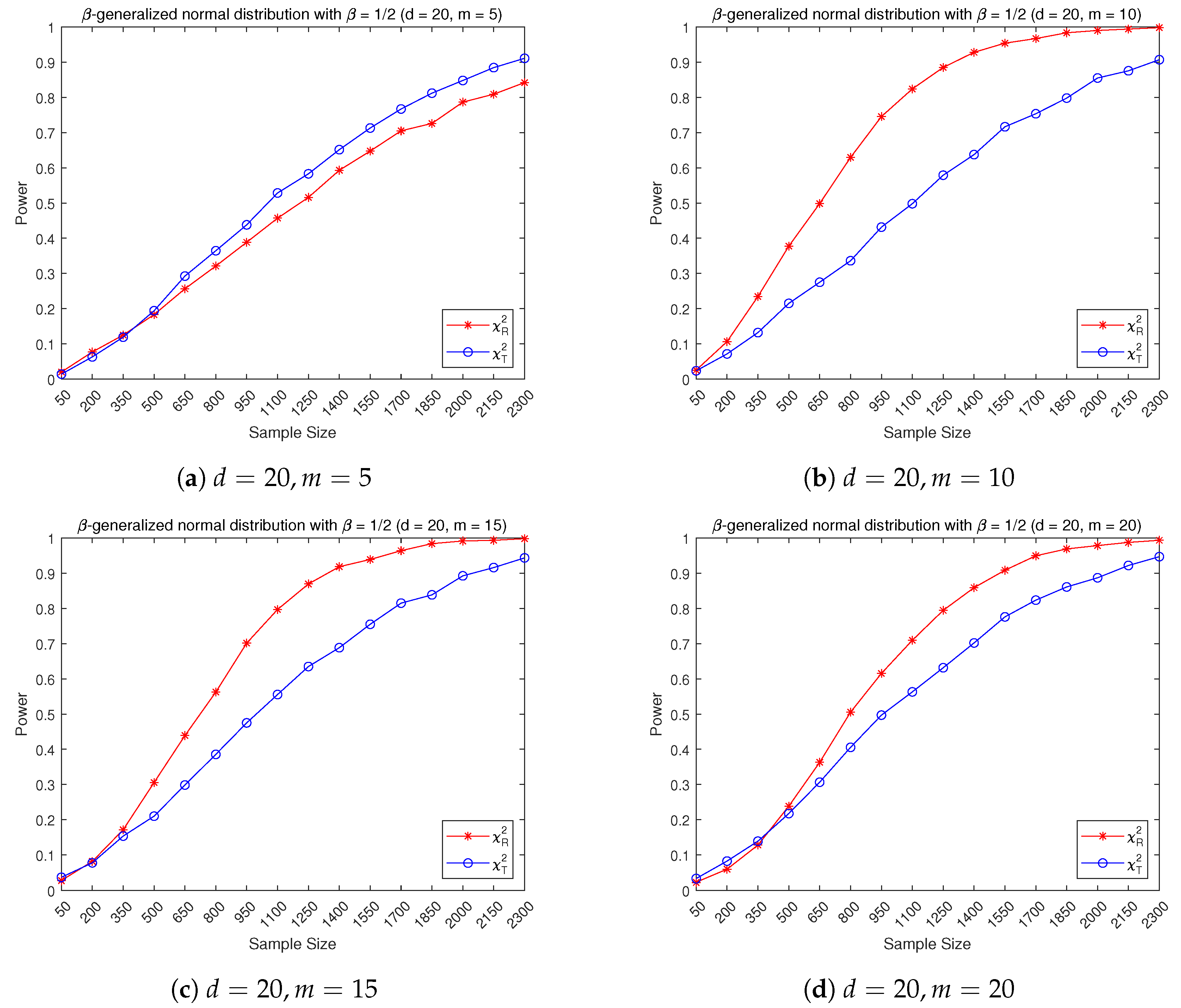
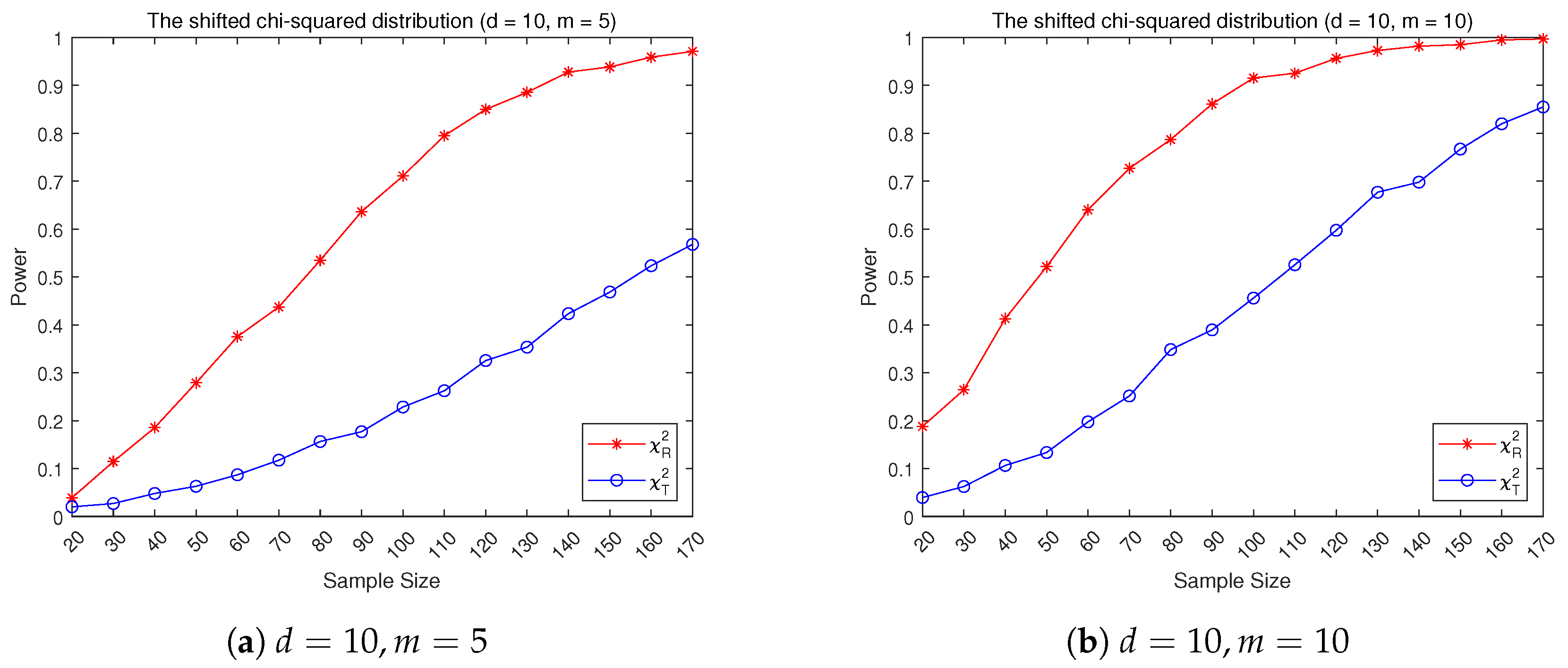
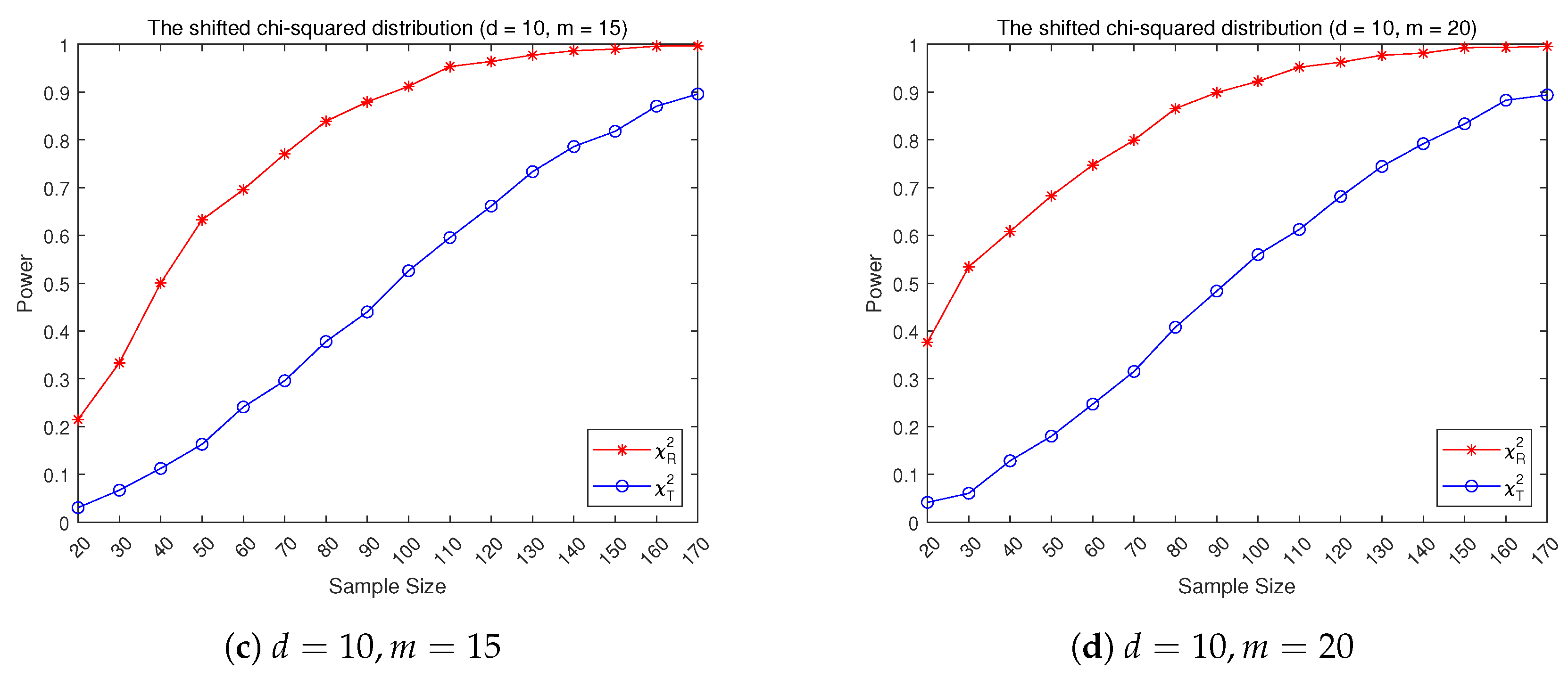
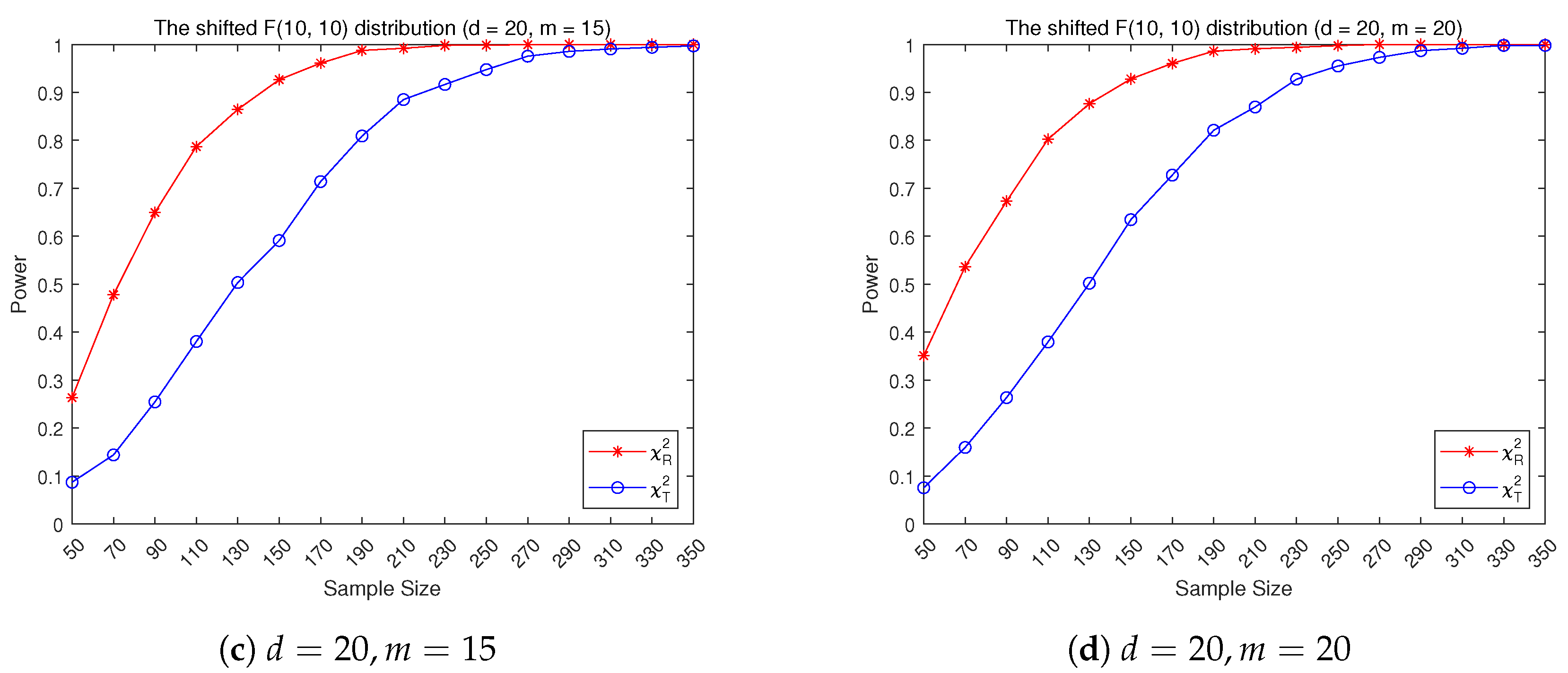
3.2. Empirical Power Performance

In order to demonstrate the power improvement of the RP chisquare over the equiprobable chisquare, we choose the following set of alternative distributions, which consists of two symmetric distributions and two asymmetric ones.

(1)

The multivariate $\beta$-generalized normal distribution constructed from the i.i.d. one-dimensional marginal $\beta$-generalized normal distribution with the density function given by

$$f_{\beta }\left(x\right)={\displaystyle \frac{{\beta }^{1-1/\beta }}{2\Gamma (1/\beta )}}exp\left(-{\displaystyle \frac{{\left|x\right|}^{\beta }}{\beta }}\right),,-\infty <x<+\infty ,\beta >0.$$

We take $\beta =1/2$.

(2)

Shifted ${\chi }^2$-distribution: ${\chi }^2\left(2\right)-2$ constructed from i.i.d. one-dimensional marginal chisquare ${\chi }^2\left(2\right)$ with $E\left[{\chi }^2\left(2\right)\right]=2$.

(3)

Shifted F-distribution $F(10,10)-10/(10-2)$; constructed from i.i.d. one-dimensional marginal $F(10,10)$ with $E\left[F\right(10,10\left)\right]=10/(10-2)$.

The two power curves for the RP chisquare ${\chi }_R^2$ (the red one in each plot) and for the equiprobable chisquare ${\chi }_T^2$ (the blue one in each plot) are plotted for four choices of the number of RPs $m=5,10,15,20$ and two choices of sample dimensions $d=10$ and $d=20$ in Figure 1, Figure 2, Figure 3, Figure 4, Figure 5 and Figure 6, as follows. Most plots (except for some of the cases of small m) show a significant power improvement of ${\chi }_R^2$ over ${\chi }_T^2$.

3.3. A Simple Comparison with Two Existing Tests

There is a relatively rich source of literature on testing spherical symmetry. Henze, Hlávka, and Meintanis (2014, [32]) proposed a new approach based on the empirical characteristic function after reviewing some existing approaches. It is commonly known that there are no simple finite-sample null distributions among all existing tests for spherical symmetry in the literature. Many existing approaches in the literature possess excellent theoretical properties with complicated null distributions for the test statistics, which limits their applications without associated statistical tables that contain critical values. Therefore, we only carry out a simple Monte Carlo comparison with two of the tests reviewed in [32] These are the Wilcoxon-type necessary test proposed by Fang, Zhu, and Bentler (1993, [27]) with critical values provided for dimension $d=3,4,5,6$, and the necessary-and-sufficient test by Baringhause [26] with percentiles given for dimensions $d=2$ and $d=3$. But [27] only provides orthogonal projection directions for $d=4$ for computing the Wilcoxon-type test. Therefore, we can only present a simple comparison between the chisquare-type tests in this paper and the two existing ones for dimensions $d=3$ and $d=4$, to limit the space of a single paper. A general Wilcoxon-type test for a two-sample problem is defined as follows ([27], pp. 35–36).

3.3.1. A Simple Comparison with a Necessary Test

Let $\{{\mathit{a}}_1,\dots ,{\mathit{a}}_m\}$ be a set of points that are uniformly scattered on the unit sphere $S_p$ in the d-dimensional Euclidean space $R^d$. For a set of d-dimensional simple random samples $\{{\mathit{x}}_1,\dots ,x_{\mathit{n}}\}$, define

$$V({\mathit{a}}_k,{\mathit{a}}_l)={\displaystyle \frac{1}{n(n-1)}}\sum _{i=1}^n\sum _{j\ne i}^{n}I\{{\mathit{a}}_k^{\prime }{x}_{\mathit{i}}<a_l^{\prime }{\mathit{x}}_j\},T_n=\underset{1\le k,l\le m,k\ne l}{min}\left\{V({\mathit{a}}_k,{\mathit{a}}_l)\right\},$$

(15)

where the notation $I\left\{A\right\}$ stands for the indicator function of a set A. Fang, Zhu, and Bentler ([27], Theorem 2) obtained the asymptotic distribution of $FZB=\sqrt{n}(T_n-1/2)$ under the null hypothesis that the sample is from a spherical distribution, and rejected the null hypothesis if $FZB<-{\lambda }_{\alpha }$ for any given d orthogonal directions in (15) under a given level $0<\alpha <1$. The orthogonal directions for approximating $T_n$ in (15) for $d=4$ are given in Table 2 and the associated critical values ($\alpha =0.01$ and $\alpha =0.05$) are given in Table 1 of [27]. Using these given directions and critical values, we carry out a simple Monte Caro comparison among our traditional equiprobable chisquare-type test ${\chi }_T^2$, the RP-based chisquare-type test ${\chi }_R^2$, and Fang, Zhu, and Bentler’s test, FZB. The null distribution is chosen as the same 4-dimensional multivariate t-distribution as used in [27], whose density function is

$${\displaystyle \frac{\Gamma \left(10\right)}{{\left(10\pi \right)}^2\Gamma \left(5\right)}}{\left(1+{\displaystyle \frac{x^{\prime }x}{10}}\right)}^{-7}.$$

The alternative distributions consists of two symmetric non-spherical distributions BGN1 = beta-generalized normal distribution with parameter $\beta =1/2$ and BGN2 = beta-generalized normal distribution with parameter $\beta =1/4$. The density function for a general beta-generalized normal distribution is given in Section 3.2. The two alternative non-symmetric distributions are SC = shifted chisquare distribution ${\chi }^2\left(2\right)-2$ and SF = shifted F-distribution $F(10,10)-10/(10-2)$ for centerization. The empirical type I error rates for different choices of the number of RPs of the Student’s t-distribution $t\left(10\right)$ are plotted against the selected sample sizes in Figure 7. The empirical power comparison among the three tests is illustrated in Figure 8 and Figure 9. Figure 7 shows that the ${\chi }_T^2$ and the FZB tests seem to control type I error rates a little bit better than the ${\chi }_R^2$ does for this specific distribution $t\left(10\right)$. Figure 8 and Figure 9 show that the FZB test is basically ineffective in testing spherical symmetry against some distributions that are symmetric about the origin, like the BGN distribution. The FZB test is generally less powerful than both ${\chi }_T^2$ and ${\chi }_R^2$ when testing spherical symmetry against severely non-spherically symmetric distributions like the shifted chisquare distribution and the shifted F-distribution. The ${\chi }_R^2$ test may improve the power performance when the number of RPs is not too big, like $m=5$ in Figure 8. It does not always dominates over the ${\chi }_T^2$ test for any choice of the number of RPs, as seen for the specific distribution $t\left(10\right)$ in Figure 7, Figure 8 and Figure 9.

3.3.2. A Simple Comparison with a Necessary-And-Sufficient Test

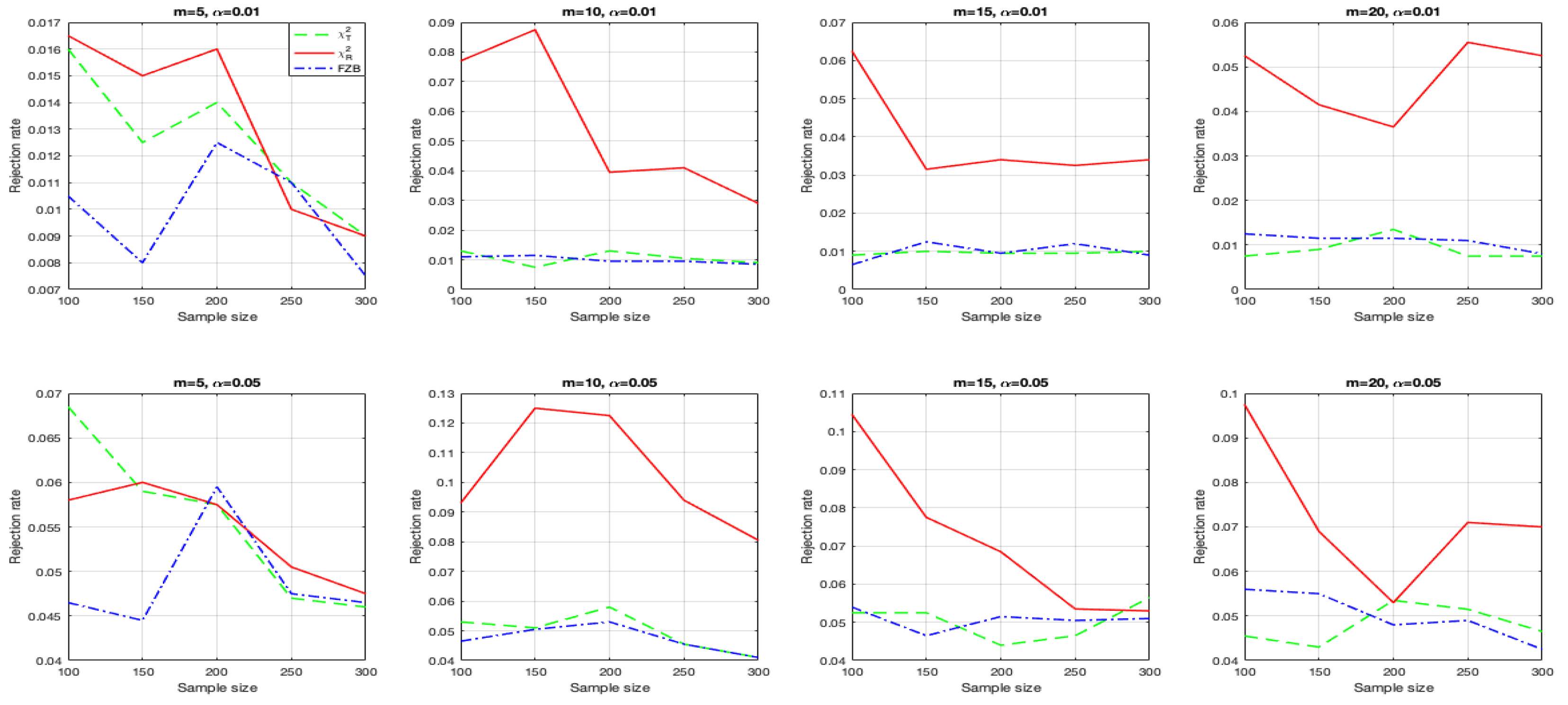
Baringhause’s necessary-and-sufficient test for spherical symmetry (9) is based on the necessary and sufficient condition:

$$\begin{array}{c}\mathrm{a} \mathrm{random} \mathrm{vector} \mathit{x}\in R^d\sim {\mathcal{S}}_d^{+}\left(\varphi \right)\mathrm{if} \mathrm{and} \mathrm{only} \mathrm{if}\\ \parallel \mathit{x}\parallel \mathrm{and} \mathit{x}/\parallel \mathit{x}\parallel \mathrm{are} \mathrm{independent} \mathrm{and} \mathit{x}/\parallel \mathit{x}\parallel \sim {\mathcal{U}}^{\left(d\right)},\end{array}$$

where ${\mathcal{S}}_d^{+}\left(\varphi \right)$ stands for the family of spherical distributions with $P(\mathit{x}=\mathbf{0})=0$ and ${\mathcal{U}}^{\left(d\right)}$ stands for the uniform distribution on the unit sphere in $R^d$, see the Corollary and Theorem 2.3 (p. 30) in [1]. For a set of i.i.d. samples $\{{\mathit{x}}_1,\dots ,{\mathit{x}}_n\}$ in $R^d$, Baringhause [26] defined the statistic

$$U_n={\displaystyle \frac{1}{n}}\sum _{i,j=1}^{n}h\left({\mathit{z}}_i^{\prime }{\mathit{z}}_j\right)min\left(1-{\displaystyle \frac{R_{n_i}-1}{n}},1-{\displaystyle \frac{R_{n_j}-1}{n}}\right),$$

(16)

where ${\mathit{z}}_i={\mathit{x}}_i/\parallel {\mathit{x}}_i\parallel$, $R_{n_i}$ stands for the rank of $\parallel {\mathit{x}}_i\parallel$ in the sequence $\{\parallel x_1\parallel ,\dots ,\parallel {\mathit{x}}_n\parallel \}$ ($i=1,\dots ,n$). Baringhause [26] recommended three choices of the scalar function $h\left(t\right)$ ($-1\le t\le 1$) for $d=3$:

$$\begin{array}{ccc}\hfill {\displaystyle h_1\left(t\right)}& =& {\displaystyle \frac{1}{16}+\frac{1}{4{\pi }^2}-\frac{arccost}{4\pi }+\frac{{(arccost)}^2}{8{\pi }^2},}\hfill \\ \hfill {\displaystyle h_2\left(t\right)}& =& {\displaystyle \frac{3}{2}-\frac{2}{\pi }\left[arccost+{(1-t^2)}^{1/2}\right],}\hfill \\ \hfill {\displaystyle h_3\left(t\right)}& =& {\displaystyle {\left(\frac{2}{\frac{17}{8}-t}\right)}^{1/2}-1.}\hfill \end{array}$$

(17)

These three choices of $h\left(t\right)$ corresponds to three statistics $U_{n1}$, $U_{n2}$, and $U_{n3}$, defined by (16), respectively. The percentiles for these three tests are given in Table 1 of [26]. Large values of any one of these three statistics imply rejection of spherical symmetry (9). We apply the six statistics ${\chi }_T^2$, ${\chi }_R^2$, FZB ([27]) with a randomly selected three orthogonal directions on the unit sphere of $R^3$, $U_{n1}$, $U_{n2}$, and $U_{n3}$ to testing spherical symmetry (9) by choosing the 3-dimensional t-distribution as in Section 3.3.1 for the null hypothesis and the three alternative distributions in Section 3.2. Under 2000 simulation replications, we summarize the empirical type I error rates for the t-distribution and the power for the four nonspherical alternative distributions in

Table 4. Empirical type I error rates and power ($\alpha =0.05$).

m	n	Test	t-distr.	$\mathit{BGN}1$	$\mathit{BGN}2$	$\mathit{SC}$	$\mathit{SF}$
$m=5$	$n=100$	${\chi }_T^2$	0.0510	0.2225	0.6130	0.9985	0.9185
		${\chi }_R^2$	0.0145	0	0.0005	0.9960	0.7550
		FZB	0	0	0	0	0
		$U_{n1}$	0.0405	0.0765	0.1530	1.0000	0.9985
		$U_{n2}$	0.0385	0.0775	0.1635	1.0000	0.9980
		$U_{n3}$	0.0450	0.0525	0.0595	1.0000	0.9985
$m=5$	$n=200$	${\chi }_T^2$	0.0475	0.4790	0.9295	0.9960	0.9995
		${\chi }_R^2$	0.0170	0.0270	0.1420	0.9940	0.9750
		FZB	0	0	0	0	0
		$U_{n1}$	0.0375	0.1165	0.4000	1.0000	1.0000
		$U_{n2}$	0.0355	0.1210	0.4305	1.0000	1.0000
		$U_{n3}$	0.0405	0.0655	0.0715	1.0000	1.0000
$m=10$	$n=100$	${\chi }_T^2$	0.0455	0.6840	0.9930	0.9450	0.9345
		${\chi }_R^2$	0.0645	0.0390	0.0135	0.8580	0.7060
		FZB	0	0	0	0	0
		$U_{n1}$	0.0355	0.0720	0.1525	0.9990	0.9985
		$U_{n2}$	0.0360	0.0725	0.1630	0.9990	0.9980
		$U_{n3}$	0.0410	0.0490	0.0570	0.9990	0.9985
$m=10$	$n=200$	${\chi }_T^2$	0.0510	0.9590	1.0000	1.0000	1.0000
		${\chi }_R^2$	0.0310	0.0060	0.0085	0.9915	0.9505
		FZB	0	0	0	0	0
		$U_{n1}$	0.0465	0.1055	0.3730	1.0000	1.0000
		$U_{n2}$	0.0485	0.1135	0.4100	1.0000	1.0000
		$U_{n3}$	0.0500	0.0510	0.0620	1.0000	1.0000

. Some empirical conclusions can be summarized:

(1)

The FZB test is completely ineffective in testing spherical symmetry in the low-dimensional ($d=3$) case when randomly choosing the orthogonal directions to approximate the statistic $T_n$ in (15). This implies that the FZB test is very sensitive for the choice of the orthogonal projection directions for approximating the null distribution of the test.

(2)

Among the six tests in Table 4, only ${\chi }_T^2$ has better performance in testing spherical symmetry for the two symmetric alternative distributions $BGN1$ and $BGN2$ (the generalized beta distribution with $\beta =1/2$ and $\beta =1/4$, respectively).

(3)

All six tests have similar power performance for the non-symmetric alternative distributions: the shifted chisquare distribution $SC$ and the shifted F-distribution $SF$, as described in Section 3.2.

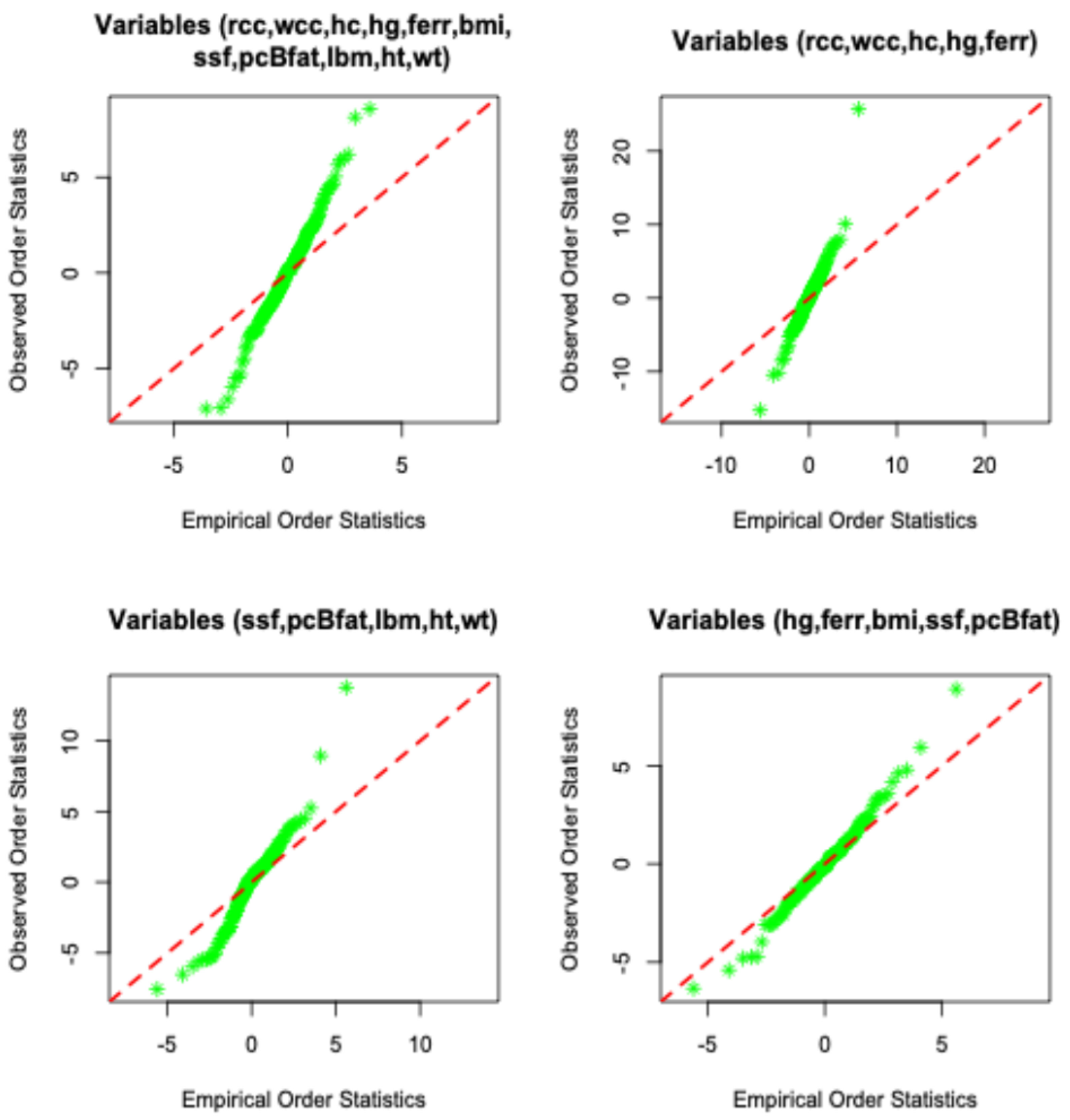
3.4. An Illustrative Example

A subset of the Australian Institute of Sport dataset was employed by Henze et al. [32] to test the two-dimensional spherical symmetry of two variables after taking the logarithm and standardization of the data. Because of the complexity of testing high-dimensional spherical symmetry, only two-dimensional simple spherical symmetry was tested in [32] Here, we want to apply the two chisquare statistics ${\chi }_R^2(m-1)$ and ${\chi }_T^2(m-1)$ ($m=$ the number of RPs) as studied in Section 3.1 and Section 3.2. The sub-dataset consists of $p=11$ variables with a sample size $n=202$. We carry out the same logarithm and standardization transformation as performed by Henze et al. [29]. The p-values from choosing different number of RPs are summarized in

Table 5. p-values from the two chisquared tests for the sport data.

	Full 11 Variables, $\mathit{d}=11$					V = (rcc, wcc, hc, hg, ferr), $\mathit{d}=5$
m	5	10	15	20	m	5	10	15	20
${\chi }_R^2$	178	427	749	1176	${\chi }_R^2$	323	918	1832	2978
p-value	0.0000	0.0000	0.0000	0.0000	p-value	0.0000	0.0000	0.0000	0.0000
${\chi }_T^2$	96	220	275	349	${\chi }_T^2$	123	207	304	355
p-value	0.0000	0.0000	0.0000	0.0000	p-value	0.0000	0.0000	0.0000	0.0000
	V = (ssf, pcBfat, lbm, ht, wt), $d=5$					V = (hg, ferr, bmi, ssf, pcBfat), $d=5$
${\chi }_R^2$	142	457	936	1693	${\chi }_R^2$	16	85	186	256
p-value	0.0000	0.0000	0.0000	0.0000	p-value	0.0003	0.0000	0.0000	0.0000
${\chi }_T^2$	83	116	150	193	${\chi }_T^2$	16	38	44	49
p-value	0.0000	0.0000	0.0000	0.0000	p-value	0.0000	0.0000	0.0000	0.0000

, where the RPs and the associated interval probabilities from the Student’s t-distribution $t(d-1)$ can be obtained from the website https://fst.uic.edu.cn/isci_en/Representative_Points/Representative_Points_for_Different_Statistical_Di.htm (accessed on 8 December 2024). The results in Table 5 strongly imply that the standardized data from different subsets (V = variables) are not from a spherical distribution for all tests.

To double-check the above non-spherical symmetry, we apply Li et al.’s [6] t-distribution Q-Q (quantile–quantile) plot to the sub-datasets in Table 5, as given by Figure 10, where all plots strongly indicate non-spherical symmetry for all sub-datasets in Table 5. This double confirms the rejection of spherical symmetry for all sub-datasets in Table 5.

4. Conclusions and a Discussion

In conclusion, this paper introduces a chisquare approach to testing spherical symmetry based on statistical representative points, offering considerable improvements over traditional equiprobable chisquare statistics in many cases. The method is particularly advantageous in high-dimensional data analysis, where the challenges of goodness-of-fit testing are compounded by the need for appropriate test statistics. By leveraging representative points, the proposed approach can enhance the power of the chisquare test, as demonstrated through a sound Monte Carlo study.

One of the key advantages of the method lies in its practicality, regardless of increasing dimensions. Although relatively large sample sizes are still required to ensure that the approximate chisquare distribution holds, the use of easily obtained representative points from an existing website simplifies the process of obtaining critical values by allowing the application of well-established chisquare tables. This makes the method more accessible and computationally efficient compared to many existing tests for spherical symmetry, which often demand more complex procedures or distribution-specific methods.

Furthermore, the real-data application demonstrates that the proposed method is somewhat robust, as different choices for the number of representative points typically lead to the same conclusion when the null hypothesis is strongly violated. This flexibility, combined with its strong performance, positions the representative-point-based approach as a valuable addition to the toolkit for testing spherical symmetry in high-dimensional settings. In essence, the method provides a fresh perspective on goodness-of-fit testing, making it a useful tool for statisticians and researchers dealing with spherical symmetry in high-dimensional data analysis.

It is noticed in the Monte Carlo study in Section 3 that, when applying the chisquare test for goodness of fit, the choice of data classification or the number of cells can impact the empirical performance of the test. This variability arises because the chisquare test is highly sensitive to how the observed data are grouped into categories. A small number of cells may result in a loss of information by oversimplifying the data distribution, potentially reducing the test’s power to detect deviations from the null hypothesis. Conversely, an excessive number of cells may lead to sparsity, where many expected frequencies become too small, violating the assumptions of the chisquare approximation and inflating the type I error rate. The choice of the number of cells should balance these two effects to ensure reliable performance. One way to address this issue is to use methods for data classification that consider the characteristics of the data and the underlying distribution. The grouping strategies based on statistical representative points or equal-probability binning can provide robust alternatives to arbitrary or equally spaced intervals. These approaches aim to create a balanced distribution of observations across cells, maintaining the validity of the test.

It should be pointed out that the RP chisquare test is a necessary one for spherical symmetry, as described by [27]. This means that if the null hypothesis of spherical symmetry is not rejected, it cannot be concluded that the sample data are from a spherical distribution. As pointed out by [27], a necessary test mainly acts to detect possible departure from the null hypothesis. Most existing tests for spherical symmetry are necessary ones, which usually result in simpler testing procedures in the sense of easy numerical computation and limiting null distribution. The RP chisquare test in this paper meets these two aspects and shows some power domination over the traditional chisquare test. Possible further research may include a comprehensive Monte Carlo comparison among some existing tests for spherical symmetry, after the work by Sakhanenko [22].

References

1. Fang, K.T.; Kotz, S.; Ng, K.W. Symmetric Multivariate and Related Distributions; Chapman and Hall: London, UK; New York, NY, USA, 1990. [Google Scholar]
2. Fang, K.T.; Zhang, Y. Generalized Multivariate Analysis; Springer: Berlin, Germany; Beijing, China, 1990. [Google Scholar]
3. Läuter, J. Exact t and F tests for analyzing studies with multiple endpoints. Biometrics 1996, 52, 964–970. [Google Scholar] [CrossRef]
4. Läuter, J.; Glimm, E.; Kropf, S. New multivariate tests for data with an inherent structure. Biom. J. 1996, 38, 5–23. [Google Scholar] [CrossRef]
5. Läuter, J.; Glimm, E.; Kropf, S. Multivariate tests based on left-spherically distributed linear scores. Ann. Statist. 1998, 26, 1972–1988. [Google Scholar]
6. Li, R.; Fang, K.T.; Zhu, L.X. Some Q-Q probability plots to test spherical and elliptical symmetry. J. Comput. Graph. Statist. 1997, 6, 435–450. [Google Scholar] [CrossRef]
7. Liang, J.; Fang, K.T. Some applications of Läuter’s technique in tests for spherical symmetry. Biom. J. 2000, 42, 923–936. [Google Scholar] [CrossRef]
8. Liang, J.; Li, R.; Fang, H.B.; Fang, K.T. Testing multinormality based on low-dimensional projection. J. Statist. Plann. Infer. 2000, 86, 129–141. [Google Scholar] [CrossRef]
9. Glimm, E.; Läuter, J. On the admissibility of stable spherical multivariate tests. J. Multivar. Anal. 2003, 86, 254–265. [Google Scholar] [CrossRef]
10. Liang, J.; Tang, M.L. Generalized F-tests for the multivariate normal mean. Comput. Statist. Data Anal. 2009, 57, 1177–1190. [Google Scholar] [CrossRef]
11. Liang, J.; Tang, M.L.; Chan, P.S. A generalized Shapiro-Wilk W Statistic for testing high-dimensional normality. J. Comput. Graph. Statist. 2009, 53, 3883–3891. [Google Scholar] [CrossRef]
12. Liang, J.; Ng, K.W. A multivariate normal plot to detect non-normality. J. Comput. Graph. Statist. 2009, 18, 52–72. [Google Scholar] [CrossRef]
13. Zellner, A. Bayesian and non-Bayesian analysis of the regression model with multivariate Student-t error terms. J. Amer. Statist. Assoc. 1976, 71, 400–405. [Google Scholar] [CrossRef]
14. Owen, J.; Rabinovitch, R. On the class of elliptical distributions and their applications to the theory of portfolio choice. J. Financ. 1983, 38, 745–752. [Google Scholar] [CrossRef]
15. Lange, K.L.; Little, R.J.A.; Taylor, J.M.G. Robust statistical modeling using the t-distribution. J. Amer. Statist. Assoc. 1989, 84, 881–896. [Google Scholar] [CrossRef]
16. Fang, K.T.; Anderson, T.W. Statistical Inference in Elliptically Contoured and Related Distributions; Allerton Press: New York, NY, USA, 1990. [Google Scholar]
17. Kariya, T.; Kurata, H. Generalized Least Squares; John Wiley & Sons Ltd.: Hoboken, NJ, USA, 2004. [Google Scholar]
18. Gupta, A.K.; Varga, T.; Bodnar, T. Elliptically Contoured Models in Statistics and Portfolio Theory; Springer: New York, NY, USA, 2013. [Google Scholar]
19. Bura, E.; Forzani, L. Sufficient reductions in regressions with elliptically contoured inverse predictors. J. Amer. Statist. Assoc. 2015, 110, 420–434. [Google Scholar] [CrossRef]
20. Dewick, P.R.; Liu, S.; Liu, Y.; Ma, T. Elliptical and skew-elliptical regression models and their applications to financial data analytics. J. Risk Fin. Manag. 2023, 16, 310. [Google Scholar] [CrossRef]
21. Gupta, A.K.; Varga, T. Elliptically Contoured Models in Statistics; Springer: Berlin/Heidelberg, Germany, 1993. [Google Scholar]
22. Sakhanenko, L. Testing for ellipsoidal symmetry: A comparison study. Comput. Statist. Data Anal. 2008, 53, 565–581. [Google Scholar] [CrossRef]
23. Babic, S.; Ley, C.; Palangetic, M. Elliptical symmetry tests in R. R J. 2021, 13, 661–672. [Google Scholar] [CrossRef]
24. Kariya, T.; Eaton, M.L. Robust tests for spherical symmetry. Ann. Statist. 1977, 5, 206–215. [Google Scholar] [CrossRef]
25. Beran, R. Testing for elliptical symmetry of a multivariate density. Ann. Statist. 1979, 7, 150–162. [Google Scholar] [CrossRef]
26. Baringhaus, L. Testing for spherical symmetry of a multivariate distribution. Ann. Statist. 1991, 19, 899–917. [Google Scholar] [CrossRef]
27. Fang, K.T.; Zhu, L.X.; Bentler, P.M. A necessary test for sphericity of a high-dimensional distribution. J. Multivar. Anal. 1993, 44, 34–55. [Google Scholar] [CrossRef]
28. Zhu, L.X.; Fang, K.T.; Zhang, J.T. A projection NT-type test for spherical symmetry of a multivariate distribution. In New Trends in Probability and Statistics; VSP: Utrecht, The Netherland; Tokyo, Japan; TEV: Uilnius, Lithuania, 1995; Volume 3, pp. 109–122. [Google Scholar]
29. Koltchinskii, V.I.; Li, L. Testing for spherical symmetry of a multivariate distribution. J. Multivar. Anal. 1998, 65, 228–244. [Google Scholar] [CrossRef]
30. Huffer, F.W.; Park, C. A test for elliptical symmetry. J. Multivar. Anal. 2007, 98, 256–281. [Google Scholar] [CrossRef]
31. Liang, J.; Fang, K.T.; Hickernell, F.J. Some necessary uniform tests for spherical symmetry. Ann. Instit. Statist. Math. 2008, 60, 679–696. [Google Scholar] [CrossRef]
32. Henze, N.; Hlávka, Z.; Meintanis, S.G. Testing for spherical symmetry via the empirical characteristic function. Stat.—A J. Theor. Appl. Stat. 2014, 48, 1282–1296. [Google Scholar] [CrossRef]
33. Albisetti, I.; Balabdaoui, F.; Holzmann, H. Testing for spherical and elliptical symmetry. J. Multivar. Anal. 2020, 180, 104667. [Google Scholar] [CrossRef]
34. Fang, K.T.; He, S.D. The Problem of Selecting a Given Number of Representative Points in a Normal Population and a Generalized Mills Ratio; Stanford Technical Report No. 327; Department of Statistics, Stanford University: Stanford, CA, USA, 1982. [Google Scholar]
35. Flury, B.A. Principal points. Biometrika 1990, 77, 33–41. [Google Scholar] [CrossRef]
36. Liang, J.; He, P.; Yang, J. Testing multivariate normality based on t-representative points. Axioms 2022, 11, 587. [Google Scholar] [CrossRef]
37. Cao, Y.; Liang, J.; Xu, L.; Kang, J. Testing multivariate normality based on beta-representative points. Mathematics 2024, 12, 1711. [Google Scholar] [CrossRef]
38. Voinov, V.; Nikulin, M.S.; Balakrishnan, N. Chisquared Goodness of Fit Tests with Applications; Academic Press: Cambridge, UK, 2013. [Google Scholar]
39. Fang, K.T. Spherical and elliptical symmetry, test of. In Encyclopedia of Statistics, 2nd ed.; John Wiley & Sons: New York, NY, USA, 2006; Volume 12, pp. 7924–7930. [Google Scholar]
40. D’Agostino, R.B.; Stephens, M.A. Goodness-of-Fit Techniques. Marcel Dekker, Inc.: New York, NY, USA; Basel, Switzerland, 1986. [Google Scholar]
41. Tashiro, D. On methods for generating uniform points on the surface of a sphere. Ann. Instit. Statist. Math. 1977, 29, 295–300. [Google Scholar] [CrossRef]
42. Fang, K.T.; Wang, Y. Number-Theoretic Methods in Statistics; Chapman and Hall: London, UK, 1994. [Google Scholar]
Figure 1. Power comparison between χ R 2 and χ T 2 for the β -normal distribution ( β = 1 / 2 , d = 10 ).
Mathematics 12 03939 g001
Figure 2. Power comparison between χ R 2 and χ T 2 for the β -normal distribution ( β = 1 / 2 , d = 20 ).
Mathematics 12 03939 g002
Figure 3. Power comparison between χ R 2 and χ T 2 for the shifted χ 2 -distribution ( d = 10 ).
Mathematics 12 03939 g003aMathematics 12 03939 g003b
Figure 4. Power comparison between χ R 2 and χ T 2 for the shifted χ 2 -distribution ( d = 20 ).
Mathematics 12 03939 g004
Figure 5. Power comparison between χ R 2 and χ T 2 for the shifted F-distribution ( d = 10 ).
Mathematics 12 03939 g005
Figure 6. Power comparison between χ R 2 and χ T 2 for the shifted F-distribution ( d = 20 ).
Mathematics 12 03939 g006aMathematics 12 03939 g006b
Figure 7. Empirical type I error rates for the three tests: the red real line is for χ R 2 , the green dashed line is for χ T 2 , and the blue dashed–dotted line is for the FZB test.
Mathematics 12 03939 g007
Figure 8. Power comparison among the three tests for the BGN distribution: the red real line is for χ R 2 , the green dashed line is for χ T 2 , and the blue dashed–dotted line is for the FZB test.
Mathematics 12 03939 g008
Figure 9. Power comparison among the three tests for the chisquare and F distributions: the red real line is for χ R 2 , the green dashed line is for χ T 2 , and the blue dashed-dotted line is for the FZB test.
Mathematics 12 03939 g009
Figure 10. t-distribution Q-Q plots for the four sub-datasets in Table 5.
Mathematics 12 03939 g010