DIAFM: An Improved and Novel Approach for Incremental Frequent Itemset Mining

Abstract

Traditional approaches to data mining are generally designed for small, centralized, and static datasets. However, when a dataset grows at an enormous rate, the algorithms become infeasible in terms of huge consumption of computational and I/O resources. Frequent itemset mining (FIM) is one of the key algorithms in data mining and finds applications in a variety of domains; however, traditional algorithms do face problems in efficiently processing large and dynamic datasets. This research introduces a distributed incremental approximation frequent itemset mining (DIAFM) algorithm that tackles the mentioned challenges using shard-based approximation within the MapReduce framework. DIAFM minimizes the computational overhead of a program by reducing dataset scans, bypassing exact support checks, and incorporating shard-level error thresholds for an appropriate trade-off between efficiency and accuracy. Extensive experiments have demonstrated that DIAFM reduces runtime by 40–60% compared to traditional methods with losses in accuracy within 1–5%, even for datasets over 500,000 transactions. Its incremental nature ensures that new data increments are handled efficiently without needing to reprocess the entire dataset, making it particularly suitable for real-time, large-scale applications such as transaction analysis and IoT data streams. These results demonstrate the scalability, robustness, and practical applicability of DIAFM and establish it as a competitive and efficient solution for mining frequent itemsets in distributed, dynamic environments.

1. Introduction

The process of identifying frequent itemsets is computationally intensive, requiring significant CPU and I/O resources. Traditional algorithms like Apriori, Eclat and FP-growth have been fundamental techniques of the frequent itemset mining (FIM) algorithm. These techniques utilized tree-based structure and multiple scans of datasets to generate frequent itemsets [1]. Despite these foremost efforts in big data analytics, these data mining algorithms faced several limitations, i.e., high computation cost, multiple scans of the dataset, memory-intensive operation, and redundant rules. These limitations minimize their application to meet the modern big data analytic requirements of scalability, efficiency, adaptability, and data management [2,3].

In modern AI applications, data are continuously generated and added to datasets, which require incremental updates to maintain the most current set of frequent itemsets [4,5]. A naive approach to handle this would involve rerunning the entire FIM algorithm on the entire dataset after each update, which is inefficient and computationally expensive [4]. To address this, incremental FIM algorithms have been proposed. These algorithms merge the results of newly processed transactions with previously mined results, though challenges arise when previously frequent itemsets become infrequent or vice versa. Effective incremental FIM algorithms minimize the need to re-evaluate past transactions, ensuring computational efficiency.

During the past decade, efforts to parallelize FIM for large-scale data have been explored, but many of these parallel algorithms suffer from network communication bottlenecks and I/O overhead [6,7]. Implementing parallel systems also introduces challenges related to load balancing, fault tolerance, and scalability. The introduction of the MapReduce framework, along with Hadoop, has helped address these challenges by providing a distributed processing environment that leverages the Hadoop distributed file system (HDFS) [8,9]. Hadoop’s ability to handle large datasets efficiently, along with its scalability across hundreds or thousands of nodes, has made it an ideal solution for large-scale data mining tasks [10,11]. The MapReduce framework automatically handles input data partitioning, parallel task execution, node failures, and inter-node communication, offering a robust and fault-tolerant system for large-scale data processing, including AI-driven applications such as predictive modeling and large-scale neural network training [12,13]. Despite much effort in FIM algorithms’ development, most traditional techniques such as Apriori, Eclat, FP-Growth, and tree-based approaches cannot scale appropriately when handling big and highly dynamic datasets. For example, Apriori and Eclat methods are always multiple passes through the data, creating unnecessary computation and memory overuses. Eclat in particular uses a vertical data structure transformation, coupled with expensive recursive intersection computations that make the approach too memory-intensive for handling large datasets, particularly on distributed computing architectures. Similarly, tree-based algorithms such as FP-Growth and CanTree are effective in static datasets but are inappropriate for dynamic datasets since they must reconstruct or update the tree structure whenever new data arrive. This not only increases computational complexity but also affects the efficiency of these algorithms for real-time or incremental mining tasks.

Furthermore, non-incremental methods cannot process increments in data properly and more often need to reprocess all the data. These conditions make the traditional algorithms inadequate for big, distributed, and real-time data environments.

Nevertheless, applications of managing data for reliable software systems have led to the emergence of key concepts over the years [14,15]. Considering the context of limitations, there is a need for a data mining mechanism that takes advantage of a phase-wise approach to data mining in an environment of distributed architecture and increased data processing.

To efficiently manage large and dynamically growing datasets, an incremental and distributed approach is required [16]. In this paper, we introduce a novel solution: distributed incremental approximation frequent itemset mining (DIAFIM), designed for a distributed parallel MapReduce environment. This is a comprehensive and advanced extension of our previous work that had a different experimental setup and a limited conceptual framework [17,18]. Compared to other MapReduce-based FIM algorithms, DIAFIM significantly enhances performance by utilizing an approximation method that balances efficiency with a controlled trade-off in accuracy. The core idea is to approximate the support of frequent itemsets within a predefined error bound, referred to as significant support, to reduce multiple scans and accelerate the mining process. DIAFM efficiently handles large datasets by minimizing dataset scans, ensuring scalability, and balancing trade-offs between computational performance and approximation accuracy, making it ideal for modern data analytics tasks. The proposed DIAFM algorithm is an improved distributed incremental approximation frequent mining, which surmounts these shortcomings by using the shard-based approximation mechanism based on the MapReduce framework. DIAFM avoids the exhaustive scan of datasets, frequent tree reconstruction, and exact support computation and focuses on balancing computational efficiency with accuracy. DIAFM ensures scalability, robustness, and suitability for dynamic datasets in distributed settings by processing only data increments and integrating shard-level error thresholds. This approach provides a practical alternative to traditional methods, filling the critical gap in handling large-scale, real-time FIM tasks. Moreover, based on experimental results and analysis of DIAFM in comparison to the frequently studied algorithm, we can conjecture that DIAFM is a relatively competitive data mining technique.

DIAFIM consists of three key phases: incremental data sharding, distributed FIM, and profile integration. In the first phase, new transactions are partitioned into shards and stored in HDFS. In the second phase, distributed FIM involves local itemset mining and approximate global itemset mining, producing an updated profile for each increment of transactions. Finally, in the profile integration phase, the updated profile is merged with the previous profile to generate the final, most up-to-date set of frequent itemsets. This approach offers a scalable, efficient solution for real-time data mining, making it suitable for modern AI applications that require continuous learning and adaptation to dynamic datasets. The following are major objectives of our research theme:

• To overcome the inefficiencies with non-incremental algorithms of FIM in treating large and dynamic datasets.
• To design DIAFM as a distributed as well as scalable algorithm for processing large datasets. It ought to reduce the runtime with less memory usage.
• To implement a shard-based process and approximation to make the least computational overhead and maintain higher accuracy levels.
• To demonstrate the performance of DIAFM to be competitive in relation to the traditional FIM algorithms in terms of execution time and memory usage.
• To extend to domains such as real-time transaction analysis, social network mining, and IoT data streams in modern analytics.

The rest of this paper is organized as follows: Section 2 highlights related work in the parallelization of frequent itemset mining algorithms with a timeline of several data mining algorithms proposed over the years. Section 3 elaborates on the theoretical, conceptual, and analytical framework of the proposed DIAFM algorithm. Experimental setup and results are separately presented in Section 4 and Section 5. Section 6 illustrates a comparative analysis of DIAFM with other algorithms followed by Section 7: “Discussion of approximation and trade-off concept”. Finally, Section 8 concludes the paper.

2. Related Work

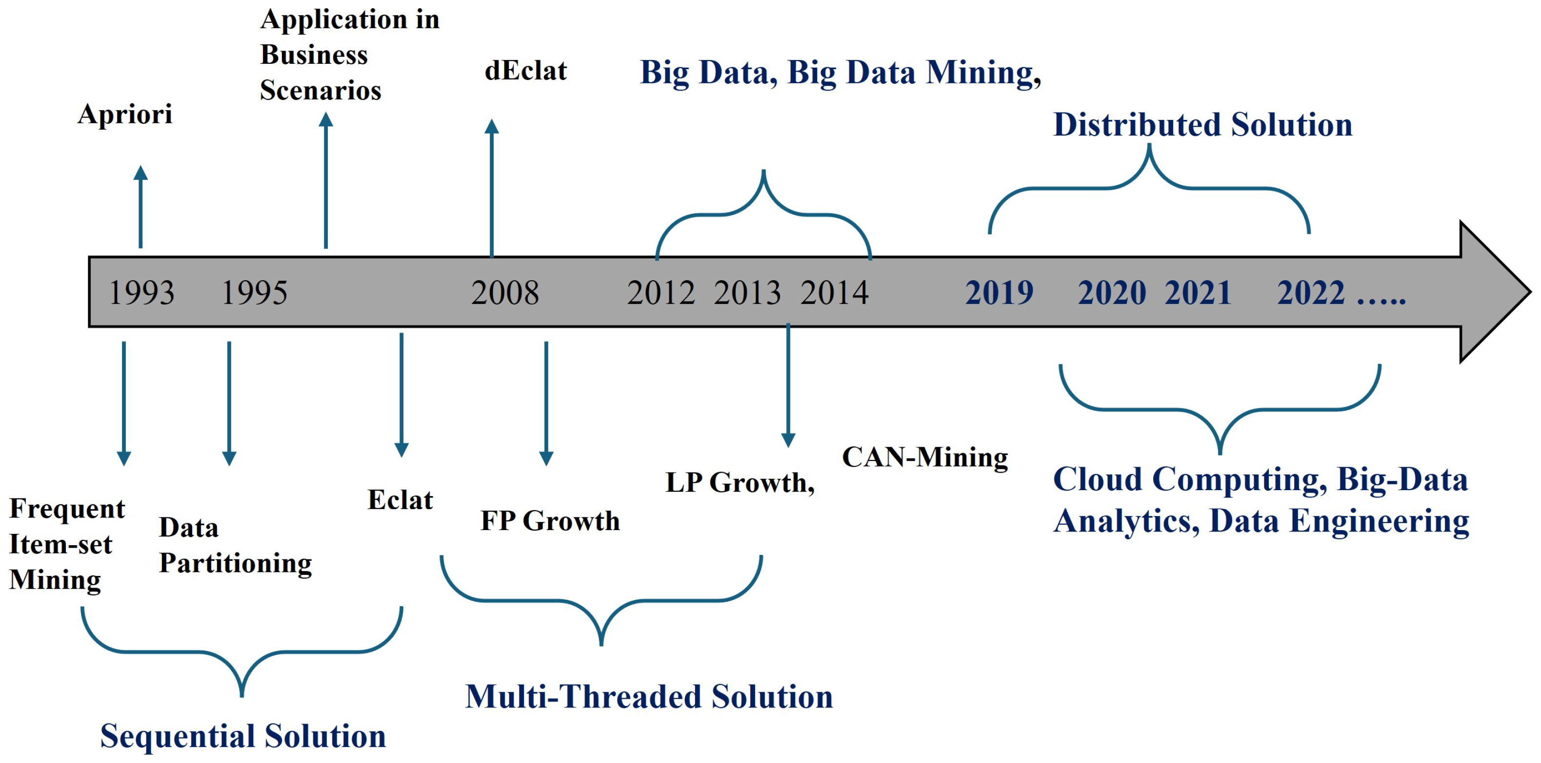
In 1993, the concept of frequent item FIM mining was first proposed in the context of market basket analysis, and since then, many improvements have been proposed. Figure 1 shows the timeline of different algorithms and trends in the evolution of data analytics over the years. The first FIM proposal in this context is known as Apriori [19], and was designed to work on a set of binary attributes, called items, and a database of transactions where each transaction was represented as a binary vector.

The provided timeline delineates the progression of data mining methodologies. It shows that the process commenced with sequential algorithms such as Apriori [20]. This algorithm pioneered frequent itemset mining and its utilization within commercial contexts, predominantly in market basket analysis [21].

In response to issues related to scalability, multi-threaded approaches including Eclat and FP-Growth were developed, presenting effective mining strategies that leverage vertical data formats and condensed data representation. Furthermore, in 2008, dEclat enhanced the performance of Eclat specifically for dense datasets. Big data that emerged over the period from 2012 to 2014 birthed algorithms such as LP Growth, which was tailor-made for extensive datasets, and CAN-Mining, emphasizing distributed scalability. In 2019 onwards, attention was shifted towards big data mining, which essentially leveraged distributed systems like Hadoop and Spark along with cloud-based platforms. Data mining turned into cloud computing, big data analytics, and data engineering in 2020–2022, with key features of scalability and in-time processing data. During this period, big data analytics found widespread applications in industries such as business operations, healthcare, and finance.

There has been a gradual improvement in technique, mechanism, and analytics since FIM was proposed. This proposal followed an interleaved breadth-first search strategy in which, at every level, candidate itemsets were derived from the itemsets mined up to that point (which were frequent). After two years, other authors proposed a variation in FIM that optimized the disk [22]. The term big data was first introduced around 2005, and it transformed all the data analytic subfields, including FIM. Over the next few years, the MapReduce programming framework was launched in industry, allowing us to process data in parallel as small pieces in distributed clusters [23]. First, the first proposal based on MapReduce came promptly while it was a version of the FP-Growth algorithm, called PFP [24], to work on distributed machines. Then, some authors have designed initial adaptations (SPC, FPC, DPC) of Apriori on MapReduce [25]. However, it was only in 2008 that truly efficient MapReduce algorithms for FIM appeared (DistECLAT and BigFIM) based on the well-known ECLAT algorithm and the other combining principles from both Apriori and Eclat [26]. Despite pioneering work on frequent itemset mining, distributed computing solutions brought a revolution in the research area of data analytics and data mining. Distributed computing of data was processed using a MapReduce-based environment. Parallel programming architectures fall into two categories: shared memory and distributed approaches. In this later type of architecture, each processor does not follow shared memory setup. Technically in this architecture, every processor has a private main memory and storage. Despite the fact that the number of MapReduce approaches and architectures for FIM continued to be conjectured [27,28]. However, these methods still do not exhibit reasonable scalability due to high workload skewness, large intermediate data, and large network communication overhead.

Although exhaustive search methodologies are traditionally used to solve the FIM problem, it is recently solved using non-exhaustive (heuristic) search methodologies inspired by MapReduce. In such proposals, the evaluation process will be parallelized since it is the most time-consuming part. It must be kept in mind that heuristic solutions have found their way onto the pages of research, for they can easily deal with continuous features without discretization at the cost of some part of the search space [29,30].

Several parallelization strategies for association rule mining have been explored, with a focus on optimizing computational efficiency, communication overhead, synchronization, and memory usage. Kumar et al. classified these strategies into three primary approaches: count distribution, data distribution, and candidate distribution [31].

The count distribution approach represents a distributed implementation of the Apriori algorithm. In this method, all distributed nodes generate the entire set of candidate itemsets and independently compute local support counts based on their partition of the dataset. A sum–reduction operation is then performed to aggregate the global support counts by exchanging these local counts across all nodes in each iteration. This method reduces communication overhead since only the support counts are shared between nodes; however, it still requires a round of communication for each iteration, which may become a bottleneck in large-scale distributed systems [32].

In contrast, the data distribution strategy assigns disjoint portions of the candidate itemsets to each node. To calculate the global support counts, each node must scan the entire dataset, including both local and remote partitions, during each iteration. While this approach ensures disjoint candidate generation, it suffers from significant I/O overhead due to repeated scanning of the entire dataset across all nodes.

The candidate distribution approach aims to reduce this overhead by ensuring that each node generates disjoint candidate itemsets, which can be processed independently. However, like the previous methods, it still requires one round of communication per iteration to synchronize the results across all nodes.

These early parallelization schemes laid the groundwork for distributed data mining but faced challenges, including high I/O overhead and frequent communication, making them less efficient for handling the vast and rapidly growing datasets of today. The emergence of the MapReduce framework, particularly in conjunction with Hadoop, has addressed many of these challenges by providing a distributed, fault-tolerant environment that automates many of the complexities involved in parallel data mining. However, issues like load balancing, scalability, and efficient management of incremental datasets in a distributed setting continue to be active areas of research. Although the FIM problem is solved in general by developing exhaustive search methodologies, It was solved recently using non-exhaustive (heuristic) search methodologies based on MapReduce. In such proposals, it is the evaluation process that needs to be parallelized since it is the most time-consuming part. It should be remembered that heuristic solutions have gained interest among researchers since they can handle continuous features without any discretization step even if they miss some part of the search space [33,34]. Recent trends in FIM are approximation-based methods, such as HyperLogLog-FIM, that significantly reduce space complexity but at the cost of exactness for efficiency. This shows how the emphasis is shifting from accuracy to resource utilization [35].

The local partitioning algorithm [36] focuses mainly on partitioning a dataset to exploit a new distributed evaluation method of FIM. It reads the dataset at most two times to find out all the frequent itemsets. In the first scan over a dataset, it generates a set of all potentially frequent itemsets. This set is a superset of all frequent itemsets; it may contain false positives. During the second scan, counters for each of these itemsets are set up and their actual support is measured in another scan over the dataset. The algorithm executes in two phases. In the first phase, the Partition algorithm logically divides the dataset into a number of non-overlapping partitions. The partitions are read one by one and all frequent itemsets for each partition are generated. Subsequently, these frequent itemsets of all the partitions are merged to generate a set of all potential frequent itemsets. In the second phase, the actual support of each itemset is generated and the frequent itemsets are identified. The portioning size is selected such that each partition can be stored in the main memory so that the partitions are read only once in each phase. Since FP-Growth was proven to outperform all of the Apriori-based algorithms, it was employed in most approaches for the parallelization of FIM [37,38].

Basically, a given dataset is partitioned into a number of smaller parts, and subsequently, a local FP-tree is built for each part in parallel. Some approaches imply multiple threads in a shared memory environment [39], but they do not address the requirement of huge memory space. One of the most famous approaches for the parallel execution of FIM in a MapReduce framework is Parallel FP-Growth (PFP) [40,41]. As an attempt for the parallel execution of the Apriori-based FIM strategy on top of a MapReduce framework, three different methods were proposed [42]. The first one, Single Pass Counting (SPC), finds out the set of frequent k-itemsets in the kth scan over a dataset scan. On the other hand, the second method, Fixed Pass Counting (FPC), finds out the set of frequent ‘k-, (k + 1)-, …, and (k + m)-’-itemsets. The third method, Dynamic Pass Counting (DPC), contemplates the workloads of nodes while it can find out as many frequent itemsets of different length as possible. To parallelize FIM in an incremental method, an efficient parallel and distributed incremental approach for mining frequent itemsets on dynamic and distributed datasets was proposed, which uses the incremental version of ZigZag algorithm [43]. By incorporating the concept of FIM and its downward closure property, this algorithm saves the repeated scans over an old dataset (D). This algorithm minimizes the communication cost for mining over a wide area network and provides novel interactive extensions for computing high-contrast frequent itemsets.

The proposed DIAFIM algorithm builds upon these ideas, introducing a more efficient approximation-based approach to frequent itemset mining in a distributed, incremental setting, reducing the need for frequent dataset scans and minimizing communication overhead while leveraging the power of the MapReduce framework [32].

3. Distributed Incremental Approximate Frequent Itemset Mining—DIAFIM

This section outlines a conceptual and analytical framework to determine frequent itemset in fast-growing dynamic data of today’s time. There are three operational phases of DIAFM, i.e., sharding of increamental data, extraction of frequent itemset and profile integration. We first theoretically define all of these concepts, taking into account the context of our study with operational and computational features.

3.1. Sharding Creation Phase

The dataset is divided into smaller, easily manageable shards, thus permitting parallel processing. This stage ensures scalability since it distributes the workload to different computational nodes, minimizing memory overhead while retaining the independence of each shard:

• Given the input of large datasets, shards are created by segregating data into small partitions.
• Each shard is stored and processed using MapReduce-based parallel computing as local itemset mining process.
• Memory management is ensured to remain efficient as smaller chunks of data are handled.
• All computational nodes take a balanced workload of handling incremental data.

3.2. Extracting Frequent Itemset from Shards

Frequently occurring itemsets are extracted by processing each shard independently, i.e., computing local itemsets using an approximation mining method. This process allows for avoiding redundant and multiple data scans and leveraging local support counts for efficiency:

• It iterates through each shard to identify unique items and their frequency counts using hash tables.
• Combines frequent 1-itemsets into higher-order itemsets (e.g., pairs, triples) to identify frequent patterns. This involves generating item combinations and evaluating their approximate support within the shard.
• Produces a list of local frequent itemsets for each shard, which includes their approximate support counts.
• Shards are processed in a parallel manner to reduce memory consumption and improve execution time.

3.3. Profile Integration

All the shard’s outputs are combined to create a global frequent itemset; in addition, maintaining the error bounds guarantees approximate accuracy along with efficient incremental architecture in managing dynamic datasets:

• It generates a global support count from the local frequent itemsets gathered from all shards.
• Error-bound refinement ensures that approximate results fall within permitted error tolerances; this reduces the need for strict verification.
• For dynamic datasets, only the new data increments are processed while earlier results are only merged without interference.
• It has a significant processing time compared to approaches like Apriori or FP-growth. Incremental updates minimize reprocessing overhead for real-time applications.

3.4. Approximation Method for Frequent Itemset Mining

The algorithm proposed is mainly aimed at focusing performance improvement through efficient approximation method. Dynamic and large datasets often entail computational complexity resulting in inaccurate support values and inadequate mining of required data. On the other hand, proposed DIAFM algorithm efficiently leverages the process of approximating the transaction with a reduced level of support. This mechanism potentially improves computational proficiency with a reduced number of data scans and relatively easier calculation in each iteration:

• Profile Update: DIAFM approximation allows for the generation of new frequent itemsets which are further updated in the data list with current increment. Technically, approximate support of each itemset is stored as a new profile.
• Merging: Data profile storing old itemset merges newly generated frequent itemsets along with their support counts into new profiles. The merging process also ensures duplication of itemset does not take place. Importantly, process further updates the data profile accordingly based on their support count.
• Profile Change Management: To handle the changes into profile due to the inclusion of incremental data. Profiling allows adequuate itemset management to ensure relevance and support level accordingly.

During the process of profile integration, DIAFM eliminates possible redundancy and provides a real-time overview of data managed into updated profiles. Thus, growing data are handled. Initially, each new transaction undergoes partitions of shards, and the algorithm makes calculations based on support values that are devised locally. This helps in the reduction in calculation over a global dataset that incurs cost and complexity. An approximation allows us to set an error bound ($\epsilon$) for each shard, i.e., each partition is acceptable within this bound and a locally partitioned dataset may differ from a global dataset by an error within this bound. After the calculation of partitions within the defined support level, locally created shards are combined while preserving the error bound. This process helps in disregarding the itemsets that fall below a threshold of ($\epsilon$), improves computational efficiency, and reduces calculation complexity at the early stage of mining. Once the process of approximation ends, DIAFM starts merging the newly mined frequent itemset with the prevalent dataset iteration. This mechanism handles the complexity of evolving data while avoiding computational overheads. Moreover, the algorithm restricts its application to continuously updating local transaction rather than scanning entire datasets, thereby making this process time and cost-effective.

In this way, the approximation process retains relevant frequent itemsets that can ensure performance gains in data analytics.

Figure 2 visually represents the process of the DIAFM operation and the core steps involved in the illustration of the algorithm. Firstly, the input dataset is divided into smaller and manageable shards. DIAFM processes each shard independently to extract the frequent itemsets. Then, there is the step of merging and updating old profiles with increasing data. Eventually, integeration forms global dataset.

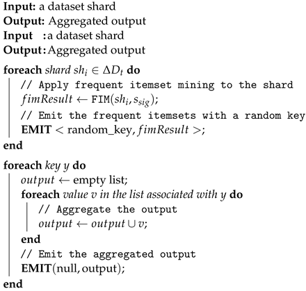
Pseudocode for DIAFM

The pseudocode (Algorithm 1) provides a high-level overview of the DIAFM algorithm. The algorithm begins by initializing the set of frequent itemsets F as empty. This is the global repository that will be incrementally updated as shards are processed. For each shard, local frequent itemsets F are mined. The input dataset D is divided into smaller subsets called shards ($Shar{d}_1,Shar{d}_2,\dots ,Shar{d}_N$). Each shard has a fixed size S. Sharding is crucial for handling large datasets as it ensures that operations can be performed on smaller, manageable subsets, thereby reducing memory usage and computational overhead. This involves identifying itemsets within the shard that meet the minimum support threshold. An approximation threshold T is applied to L, filtering itemsets based on their likelihood of being globally frequent. This step reduces the computational burden of exact support calculations and balances precision and efficiency.

Algorithm 1: Dynamic incremental approximation frequent mining (DIAFM)

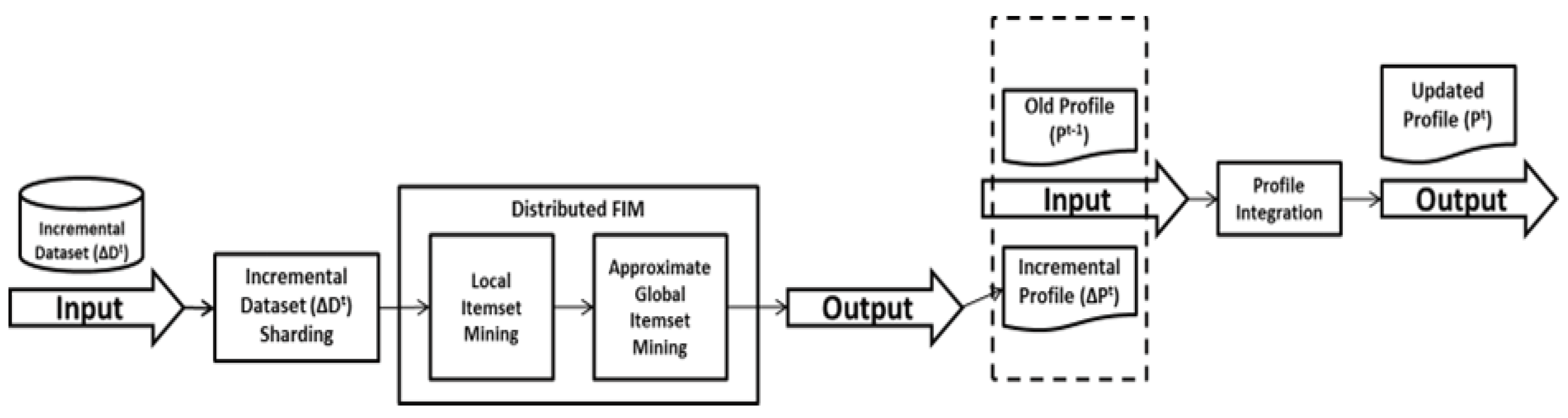
3.5. DIAFM: Implementation Framework

The FIM task can be stated as follows: Given a set of distinct items, denoted as itemset I, and a dynamic dataset $D_t$ at some time t, which is defined by its previous set $D_{t-1}$ and a new increment $\Delta D_t$, where both $D_{t-1}$ and $\Delta D_t$ consist of transactions $T_1,T_2,T_3,\dots ,T_n$ at times $t-1$ and t, respectively, each transaction in $D_t$ has a unique transaction identity ($tid$). Let $P_{t-1}$ and $\Delta P_t$ denote the sets of frequent itemsets of $D_{t-1}$ and $\Delta D_t$, respectively. These sets of frequent itemsets are called profiles of their respective datasets. The output of the proposed algorithm, i.e., the updated profile $P_t$ at time t, is obtained after integrating $P_{t-1}$ and $\Delta P_t$.

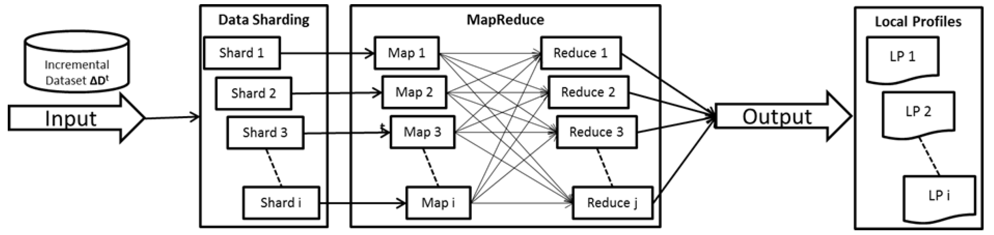
There are three major phases proposed in the execution of the algorithm: ($\Delta D_t$) the first phase involves the sharding of the initial data provided. In the second phase, the process of partitioning comes into effect ($\Delta D_t$), which typically follows the mechanism of distributed FIM. Third phase is of profile integration, where different datasets generated from phases 1 and 2, respectively, are integrated. The distributed FIM phase is achieved by chaining two consecutive MapReduce jobs: local itemset mining and approximate global itemset mining. In the profile integration phase, profiles $P_{t-1}$ and $\Delta P_t$ are merged to obtain the updated profile $P_t$. The overall workflow of the algorithm is shown in Figure 3.

To demonstrate the idea of our approach, we have used an example in this paper which shows the overall working of each phase individually. All the major steps of the DIAFIM are illustrated with an example, and for the given example, assume that the number of map and reduce nodes configured in the Hadoop cluster is 2. $P_{t-1}$ was generated from $D_{t-1}$ at some time $t-1$. The values of the minimum support variables $s_{sig}$ and $s_{min}$ are 25% and 50%, respectively.

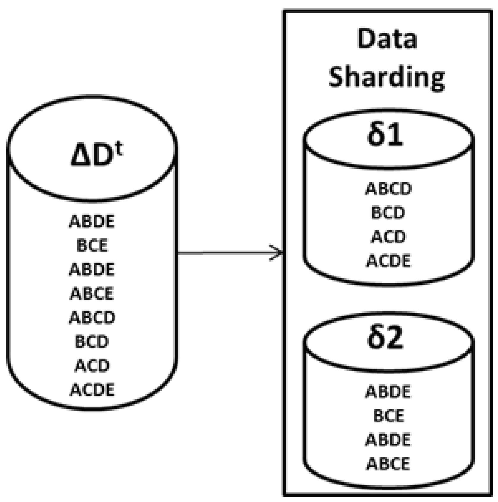
3.6. Incremental Data ($\Delta D_t$) Sharding

DIAFIM partitions the set of newly generated transactions $\Delta D_t$ into a number of equal-sized non-overlapping shards ${\delta }_1,{\delta }_2,{\delta }_3,\dots ,{\delta }_i$. Those shards are then uploaded to HDFS and assigned to a map node available in the Hadoop system. Subsequently, every map node reads its assigned shard(s) in parallel. The size of a shard depends upon the density of the dataset, Hadoop configurations, and the value of $s_{min}$. The CPU and memory requirements of a Map function turn out to be high if the size of data shards is big, the initial input minimum support value is low, the average length of the transactions is long, and the density of the incoming data is high. If the size of a data shard is large, then it will require huge memory during the execution of MapReduce jobs. In contrast, small-sized shards will result in a large and excessive number of MapReduce tasks, thus increasing the required processing time. If the number of shards produced during the incremental data ($\Delta D_t$) sharding phase is less than the number of available map nodes, then it will result in unused or idle map nodes. To maximize the proficient throughput of the MapReduce environment, the size of each data shard should be optimal.

An example for the incremental data ($\Delta D_t$) sharding phase is shown in Figure 4.

The above figure is an example of how incremental data sharding is performed over any dataset. Figure 4 illustrates that ($\Delta D_t$) having nine transactions can supposedly cause incoming incremental data to be partitioned in non-overlapping shards ${\delta }_1,{\delta }_2$ with corresponding four and five transactions, while maintaining size and efficiency. This process ensures efficient resource utilization in a distributed system.

3.7. Distributed FIM

The distributed FIM phase encompasses two chaining MapReduce jobs: local itemset mining and approximate global itemset mining. The local itemset mining phase employs a user-defined threshold value $s_{sig}$. Based on the $s_{min}$ value, the support values of the global frequent itemsets will not be accurate because a local frequent itemset of a single dataset shard ${\delta }_1$ might not be frequent in other shards ${\delta }_2,{\delta }_3,\dots ,{\delta }_i$; such a result set is called a false-positive result set. To prune out globally infrequent itemsets and to obtain the precise support values of the global frequent itemsets, one more scan over the dataset is needed. On the other hand, after pruning the small itemsets with the aggregated global support less than $s_{min}$, we will obtain a false-negative result set, namely the itemsets that are actually globally frequent, but because of the lower frequency in other shards, those itemsets will turn out to be infrequent. The only way to obtain a complete set of frequent itemsets with their corresponding precise support values and without the need for the second scan over the dataset would be by discarding a minimum support value; that is, to perform mining on all frequent itemsets with the absolute support value of 1. However, that approach is obviously infeasible for large transactions due to the exponential nature of subset generation. More specifically, a transaction T of length K generates $2^k$ subsets, which obviously cannot be calculated within a reasonable amount of time. By providing a flexible trade-off between processing time and FIM accuracy, the second scan over the dataset can be eliminated by using a refined version of the approximation method proposed in the data mining research literature [44,45]. This processing time and FIM accuracy trade-off is achieved by introducing a new user-defined threshold variable $s_{sig}$, which is lower than $s_{min}$. Executing FIM on each data shard produces a set of local frequent itemsets for the given local minimum support value of $s_{sig}$. The lower the value of $s_{sig}$, the more accurate results we obtain, and vice versa. We may still obtain false-negative results, but again, the processing time and FIM accuracy trade-off can be controlled by changing the local minimum support value of $s_{sig}$.

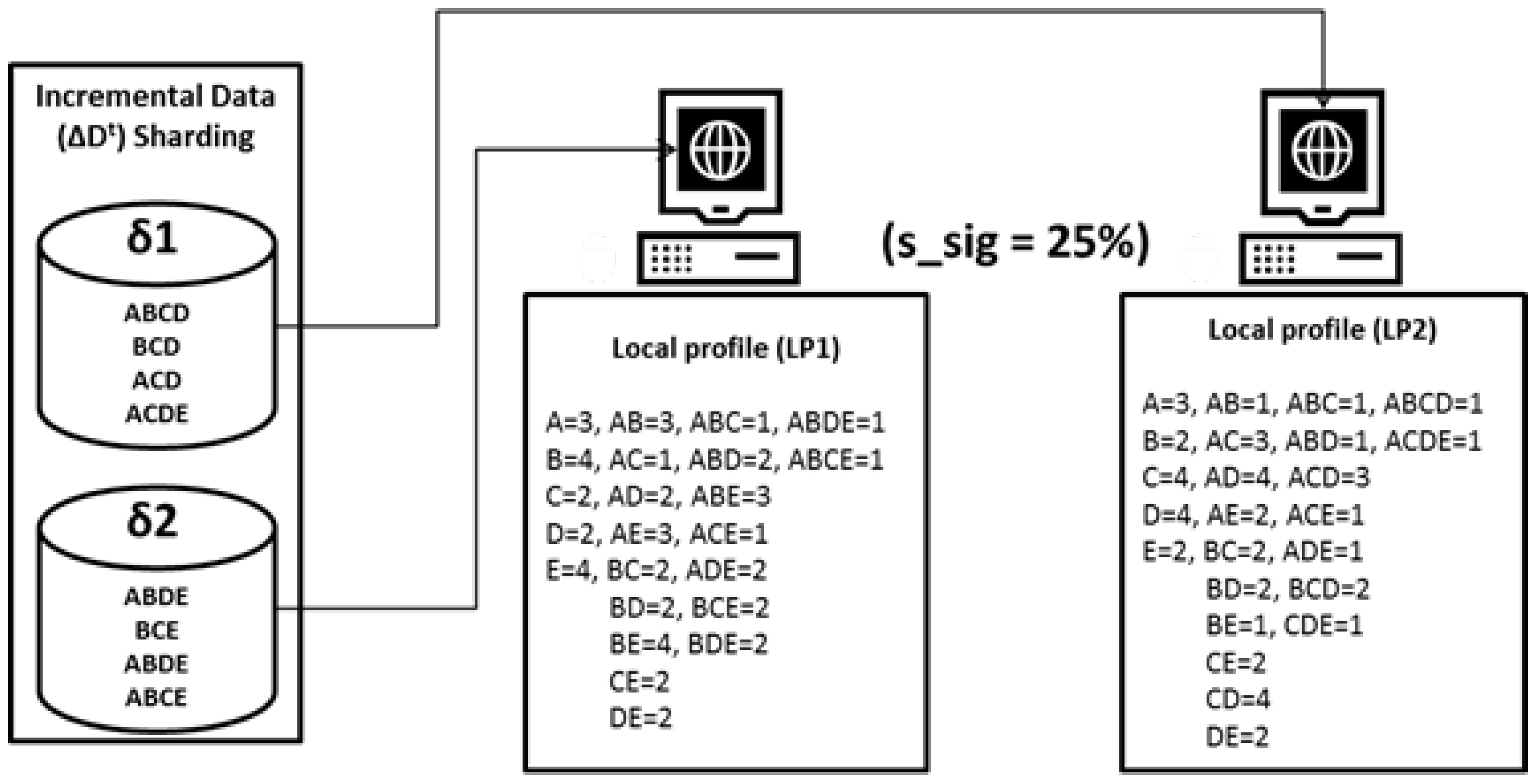
In the local itemset mining phase, all the frequent itemsets of each data shard are identified individually by each map node. Frequent itemsets identified in each data shard are called local frequent itemsets. All the local frequent itemsets are kept in HDFS as local profiles $L{P}_i$. The overall workflow of the local itemset mining phase is shown in Figure 5.

Given a minimum support value of $s_{sig}$, the map function of each node executes an FIM algorithm on its assigned data shard. The outputs of map nodes are subsequently sent as input to the reducers as the <key, value> pair. Any FIM algorithm can be used as the map function of this phase. The key in the <key, value> pair is a number between 1 and the number of reducers configured in the Hadoop system, and the value is the identified frequent itemset.

The reducer function reads the output of a map node, i.e., in the form of a <key, value> pair. In addition, the reducer function aggregates the support count of each itemset with the same key and sends the output to HDFS as local profiles $L{P}_i$. The MapReduce-based pseudocode for the local itemset mining phase of the distributed FIM is shown in Algorithm 2.

Algorithm 2: Mapper-Reducer Class

In continuation of the example of incremental data $(\Delta D_t)$ sharding presented in Figure 4, the example for the increamental itemset mining is illustrated in Figure 6. In the increamental itemset mining phase, $s_{sig}$ is used as the minimum support threshold variable. Itemsets with a support value less than  25%, ($s_{sig}$) are discarded as infrequent. Whereas itemsets with a support value greater than or equal to 25% are updated in their respective local profiles. The outputs of the local itemset mining phase are two local profiles, LP1 and LP2, generated from ${\delta }_1$ and ${\delta }_2$, respectively. LP1 and LP2 are sent to HDFS to be further processed in the next phase of the algorithm.

Once all the local profiles $\left(L{P}_i\right)$ recreated in the local itemset mining phase, the distributed procedure can be used to find the global frequent itemsets by aggregating the counts of each local frequent itemset.The approximate global itemset mining phase is primarily incorporated in our approach to cope up with the problem of huge memory requirements. If the number of itemsets produced by the local itemset mining phase in local profile is huge, writing the output of each itemset together with its support value at the same time results in poor performance and high memory consumption. This phase starts by reading all the local profiles $\left(L{P}_i\right)$, where $i=1,2,3,\cdots ,n,$ from HDFS and maps all the itemsets and their support value in sequence by reading the input line by line. In this phase, the map function performs processing and simply outputs the itemset as the key and its support as the value, i.e., in a <key, value> pair to the HDFS. On the other hand, the reducer reads the output of the map function from HDFS and aggregates the support values of the same itemsets. If the aggregated support value of an itemset is greater than the minimum support value $s_{m}in$, then the itemset is considered as globally frequent and is sent to HDFS with its support value; otherwise, the itemset is discarded and considered to be infrequent. Figure 7 shows the workflow of approximate global itemset mining.

Since our approach skips the second scan over the old dataset $\left(D_{t-1}\right)$, it allows for some false-positive and false-negative results. The correctness of our approach can be analyzed by the following lemma, which is the basic theoretical foundation of the distributed FIM problem [19].

Lemma 1.

A global frequent itemset must be locally frequent in at least one shard (δ).

Proof. 

Let C be an itemset. Let $suppor{t}_i\left(C\right)$ denote the absolute support of itemset C in the data shard ${\delta }_i$, where $i=1,2,3,\dots ,n$.

If

$$suppor{t}_i\left(C\right)<s_{\min }\times \left|\delta \right|\mathrm{for}\mathrm{all}i=1,2,3,\dots ,n$$

then

$$support\left(C\right)<s_{\min }\times \left|D\right|.$$

Since

$$support\left(C\right)=\sum _{i=1}^{n}suppor{t}_i\left(C\right)\mathrm{and}\left|D\right|=\sum _{i=1}^n\left|{\delta }_i\right|,$$

it follows that C cannot be globally frequent. Therefore, if C is a global frequent itemset, it must be locally frequent in some data shard ${\delta }_i$.    □

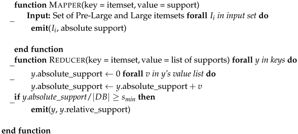
The MapReduce-based pseudocode for the approximate global itemset mining phase of distributed FIM is shown in Algorithm 3 below.

Algorithm 3: Mapper and Reducer

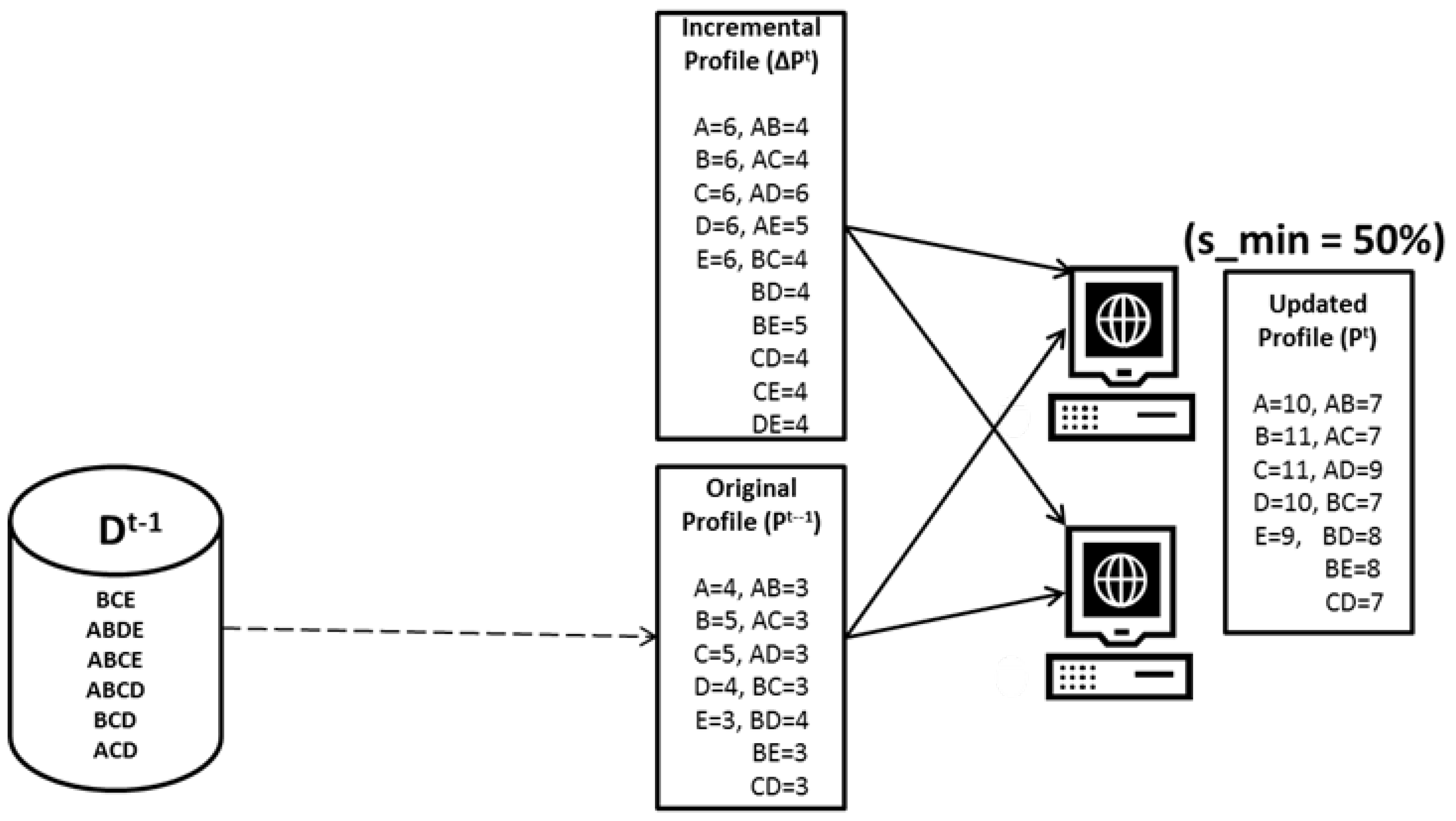
3.8. Integration ($Pt-1+\Delta Pt\to Pt$)

In this phase, the old profile $Pt-1$ is merged with the profile $\Delta Pt$ of a new increment $\Delta Dt$ to obtain the most up-to-date profile of frequent itemsets $Pt$. The incremental profile $\Delta Pt$ is stored in memory to be distributed among the nodes in the Hadoop system. The old profile $Pt-1$ is then sent to the map function and checked against the incremental profile $\Delta Pt$ such that if the itemset exists in both the profiles, i.e., $\Delta Pt-1$ and $\Delta Pt$, then the support value of that itemset from both profiles is aggregated and subsequently sent to the reducer function. Otherwise, the support value of that itemset is checked again with respect to the size of the new increment $\Delta Dt$. If the itemset turns out to be frequent, then it is sent to the reducer function, and otherwise, it is considered as infrequent and discarded. Without any additional processing, reducers send their inputs directly to HDFS as the updated profile $Pt$. The workflow of the profile integration phase is shown in Figure 8.

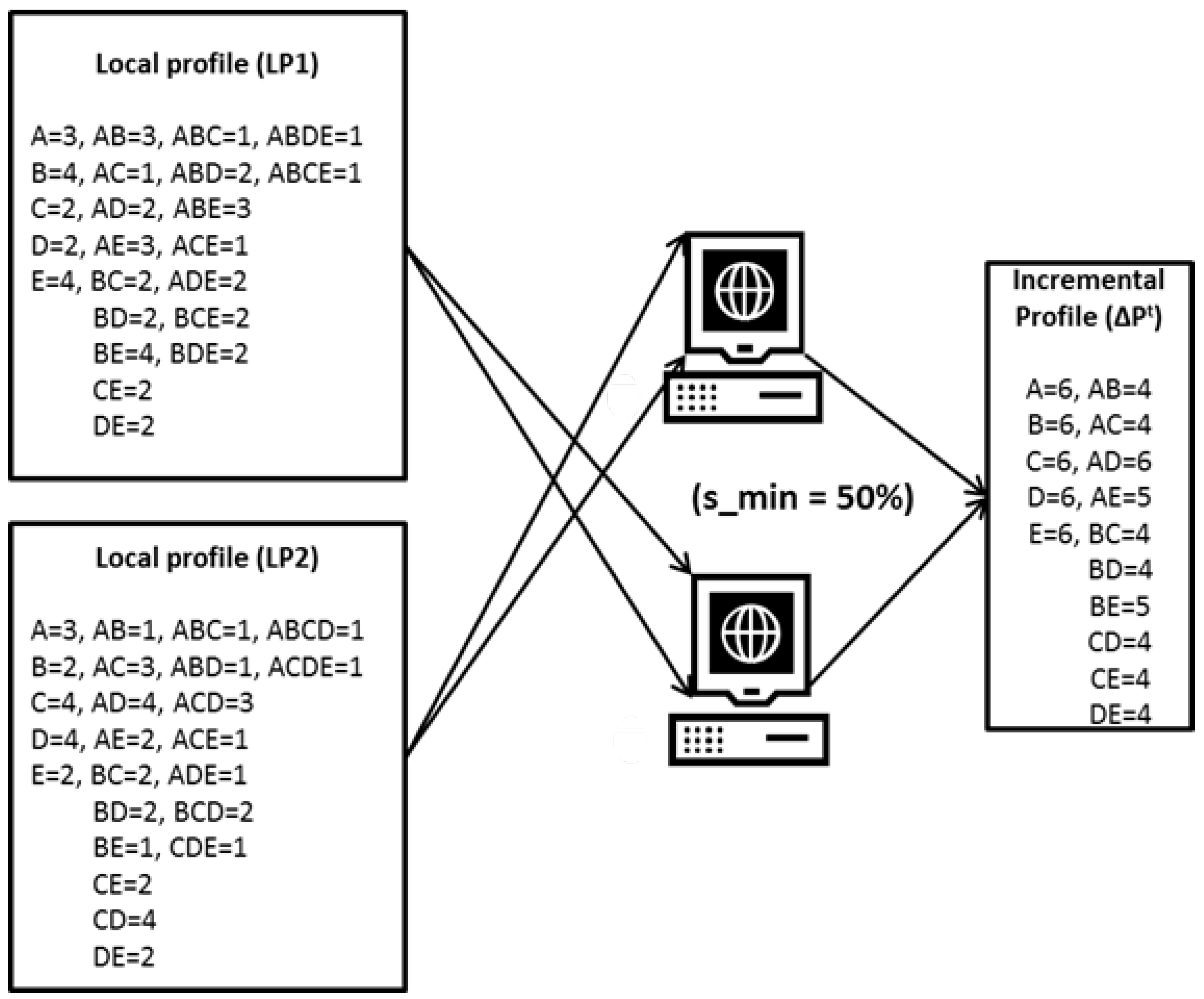
In this approach, using the minimum support value of $s_{min}$, when FIM is performed on both the old ($Dt-1$) and incremental ($\Delta Dt$) sets of transactions, during profile integration, an itemset may fall into four different cases as discussed below:

• If an itemset is frequent in both the old profile ($Pt-1$) and the incremental profile ($\Delta Pt$), it will remain frequent in the updated profile ($Pt$). To obtain the final support count, the support count of an itemset in the old profile ($Pt-1$) is aggregated with the corresponding support count in the incremental profile ($\Delta Pt$).
• Likewise, if an itemset is frequent in neither the old ($Pt-1$) nor the incremental ($\Delta Pt$) profiles, the itemset is ignored as an infrequent itemset because it will remain infrequent in the updated profile ($Pt$).
• In contrast, having an itemset that is frequent in the old profile ($Pt-1$) but not frequent in the incremental profile ($\Delta Pt$) or vice versa may increase or decrease the existing number of frequent itemsets. The support count of an itemset in the old profile ($Pt-1$) is aggregated with the corresponding support count in the incremental profile ($\Delta Pt$). To check whether an itemset is frequent or not, the aggregated support count is then compared with the minimum threshold value $s_{min}$.
• If the itemset is infrequent in an old profile ($Pt-1$) but it is frequent in the incremental profile ($\Delta Pt$), we use the theorem proposed in [46] to take care of this case. The theorem is as follows.

Theorem 1.

Let $\left|D\right|$ and |Inc| be the frequent itemsets in the old ($Pt-1$) and incremental ($\Delta Pt$) datasets, respectively. If $\left|Inc\right|\le {\displaystyle \frac{(s_{min}-s_{sig})\left|D\right|}{1-s_{min}}}$, an itemset that is infrequent in the old profile ($Pt-1$) but is frequent in the incremental profile ($\Delta Pt$) can never be frequent in the updated profile ($Pt$).

Extending the example illustrated in Figure 7 of the approximate global itemset mining phase, Figure 9 shows the example of profile integration. In the profile integration phase, $Pt-1$ and $\Delta Pt$ are merged such that the itemset that is present in both $Pt-1$ and $\Delta Pt$ is considered as frequent and written directly in the updated profile $Pt$, while the minimum support values of the rest of the itemsets with the same keys are aggregated and checked against the minimum support threshold value of $s_{sig}$ with respect to the size of new incremental transactions. $Pt$ is the final output of DIAFIM and will be considered as the old profile $Pt-1$ for the next set of incremental transactions at some time t.

3.9. Theoretical Complexity of DIAFM

Analyzing the theoretical complexity of the code using asymptotic notation requires examining the different steps, especially with respect to the dynamic incremental approach to frequent mining (DIAFM) principles and frequent itemset mining (FIM) algorithms.

As explained in the theoretical and analytical framework of DIAFM that spans across three phases, we have essentially devised a theoretical complexity analysis separately for all phases.

Shard Creation: Shard creation is a process of partitioning n number of transactions in k smaller sizes. If s is the number of shards, then the approximated shards are to be denoted as i.e., s $\approx {\displaystyle \frac{n}{k}}$, with m number of transactions averaged in each shard. This slicing of the transaction list and the making of partitions would asymptotically cost $\mathcal{O}\left(n\right)$.

Extracting Unique Items: The methodology of extracting unique items requires iterating over each shard s consisting of m number of items. This task would be of $\mathcal{O}(k·m)$ computation for each shard. Therefore, for n number of shards, it becomes $\mathcal{O}(n·m)$.

Generating Candidate Itemsets: As the first step, we compute 1-itemset occurrences, which are recorded in a dictionary. In programming terms, a hash variable carries out lookup and insertion tasks for each item m of the shards and then for all n shards. This makes the complexity of 1-itemset to be $\mathcal{O}(n·m)$. Secondly, we generalize the higher-order itemset generation process. Let f be the number of frequent itemsets generated and merged subsequently for all the shards:

• Creating a combination of f itemsets requires the complexity of $\mathcal{O}\left(f^2\right)$, whereas $f\le m$, forms an approximate complexity of $\mathcal{O}\left(m^2\right)$.
• Since we have s representing the shard created, its complexity within candidate-sets becomes $\mathcal{O}(s·m^2)$.

• However, as mentioned earlier, s is ${\displaystyle \frac{n}{k}}$ (shard creation) and we have also derived higher-order candidate generation complexity as $\mathcal{O}(s·m^2)$. Thus complexity of higher-order candidate generation of all the shards can be asymptotically respresented as: $\mathcal{O}\left({\displaystyle \frac{n}{k}}·m^2\right)$.

Combining over all complexity: As previously explained in the theory of devising the DIAFM algorithm, key steps of the algorithm involve the creation of shards, extracting the frequent itemset in profiles and integerizing all the profiles. Therefore, merging the overall complexity of all the steps results in the following equation:

$$\mathcal{O}\left(n\right)+\mathcal{O}(n·m)+\mathcal{O}(n·m)+\mathcal{O}\left({\displaystyle \frac{n}{k}}·m^2\right).$$

This simplifies to:

$$\mathcal{O}(n·m)+\mathcal{O}\left({\displaystyle \frac{n}{k}}·m^2\right).$$

The DIAFM method makes this possible by dealing with each shard in an independent manner, thus allowing frequent itemset mining to be applied to extremely large datasets. However, the complexity still scales with the number of transactions and average transaction size. Shards also provide a type of parallel processing, which can make computation much faster in practice, although asymptotically the complexity does not change.

The space complexity of DIAFM is dominated by the need to store shard-level candidate itemsets and global frequent itemsets. For each shard, the storage requirement is $O(S·k)$, while the global aggregation requires $O\left(m\right)$. Therefore, the space complexity can be expressed as:

$$O(N·S·k)+O\left(m\right).$$

The complexity analysis contains both time and space components that break down the dependence on dataset size, shard size, and other factors. It gives a clear quantitative explanation of the advantages of DIAFM. Unlike algorithms such as Apriori and FP-Growth, DIAFM operates with smaller shards as opposed to a huge dataset, meaning that this algorithm uses relatively minimal amounts of memory compared to other similar algorithms.

Although DIAFM presents reasonable scalability and less computational overhead, its approximation approach may lead to slight inaccuracies in the computation of global support.

Table 1. Comparison of time and space complexity.

Algorithm	Time Complexity	Space Complexity	Remarks
Apriori	$O\left(2^n\right)$	$O(n·|D\left|\right)$	High overhead for large datasets
Eclat	$O\left(2^n\right)$	$O(n·|D\left|\right)$	Efficient for sparse datasets
FP-Growth	$O\left(2^n\right)$	$O\left(\right|FP\text{-}tree\left|\right)$	Memory-efficient but computationally intensive
TreeProjection	$O\left(n^2\right)$	$O(n·|D\left|\right)$	Relatively faster for dense datasets
DIAFM	$O(N·S·k)$	$O(N·S·k)$	Scalable but with approximation errors
HyperLogLog-FIM (Approx.)	$O(N·\log S)$	$O(N·\log S)$	Approximate with minimal memory usage

Notations: n: Number of unique items in the dataset. $\left|D\right|$: Total size of the dataset. $\left|FP\text{-}tree\right|$: Size of the FP-tree structure. N: Number of shards (subdivisions of the dataset). S: Size of each shard. k: Number of iterations required for the mining process. $\log S$: Logarithmic factor representing compact dataset size approximation.

below compares time and space complexity for popular algorithms: Apriori, Eclat, FP-Growth, and TreeProjection. We can evidently state that DIAFM achieves a trade-off between computational efficiency and scalability. While Apriori and FP-Growth cannot be applied to large datasets because of exponential time and space requirements, DIAFM makes use of sharding and approximation to deal with the complexity. Algorithms like HyperLogLog-FIM, using probabilistic counting, might offer better space efficiency at the cost of accuracy. Table 1 compares DIAFM with other prevalent algorithms, taking into account relative advantages and shortcomings. Algorithms like Apriori and FP-Growth are highlighted for their exponential complexity, while HyperLogLog-FIM is noted for its probabilistic efficiency.

4. Experimental Setup

The DIAFM experimental work is based on a comprehensive assessment of the algorithm to determine speed, scalability, and efficiency. In the local itemset mining phase, FP-Growth was employed as the frequent itemset mining (FIM) algorithm, and the experiments were performed using cloud distributed environment comprising 4 nodes. PySpark was coded to handle several essential operations of DIAFM, sharding, data mining, and integration of profiles over each node. Each node comprised of compatable specifications that include Google Compute Engine n1-standard-4 having vCPUs (Intel Xeon Cascade Lake architecture), a RAM of 15 GB, and a disk storage of 100 GB SSD per node. Each node was further deployed using Linux distribution of Ubuntu 20.04 LTS with the latest cluster management: Google Dataproc. Additionally, the Google Cloud Storage service was employed to reduce latency and accelerate the processing of large datasets.

Finally, a PySpark script for DIAFIM was written, incorporating sharding, mining, and profiling steps, and uploaded to the GCS bucket. Such an experimental setup ensures scalability and computation efficiency by leveraging distributed data processing on Google Cloud.

We particularly opted for a robust experimental setup as Google Cloud has certain salient features, i.e., scalability for large datasets acquired from Kaggle and generated using Python-3.12.6 (https://www.python.org/downloads/, accessed on 6 September 2024) pandas library with sizing of 1 to 10 million; high-performance virtual machine, like VCPUs, ensuring effective memory usage and balanced computational power; data storage using GCP service to avoid any turbulence of reading large data; and cost-effectiveness. We have made all our experimental data publicly available in the Github repository. (https://github.com/Analyzer2210cau/DIAFM-Experiment, accessed on 8 November 2024) for replication and reproduction purposes.

4.1. Synthetic Datasets

To provide support for the objectives of this study, five distinct synthetic datasets were generated, simulating various real-world scenarios. These datasets, each 4 million records long, were envisaged to represent four different domains: e-commerce transactions, bank transactions, healthcare appointments, retail store sales, and utility bill payments. The synthetic nature of the datasets ensures privacy but still holds the required structural integrity for analysis. Below are detailed definitions of each dataset along with their attributes:

E-commerce Transaction Dataset-T10I4D10M: This dataset simulates online shopping behavior and captures essential details about transactions.

• TransactionID: A unique identifier for each transaction (e.g., TXN0000001).
• CustomerID: A unique identifier for customers (e.g., CUST12345), reused across multiple transactions to reflect repeat customers.
• ProductID: Aliases for purchased items, randomly sampled from 500 product codes.
• TransactionDate: The date of the transaction, randomly spread over the last two years.
• TransactionAmount: The monetary value of the transaction, ranging between USD 10 and USD 1000.
• PaymentMethod: The type of payment used, such as credit card, PayPal, cash, or bank transfer.
• Status: The status of the transaction, either Success or Failed.

Bank Transaction Dataset-T15I4D10M: This dataset models bank account activities, representing different transaction types and their financial implications:

• TransactionID: A unique identifier for each bank transaction (e.g., TXN0000001).
• AccountID: Unique identifiers for bank accounts (e.g., ACC54321), reflecting multiple transactions for the same account.
• TransactionDate: The timestamp for each transaction, spanning the last year.
• TransactionAmount: The amount involved in the transaction, ranging from USD 100 to USD 10,000.
• TransactionType: Type of transaction, categorized as Deposit, Withdrawal, or Transfer.
• Balance: Account balance post-transaction, randomly generated between USD 1000 and USD 50,000.
• Branch: The branch location of the transaction (e.g., New York, London, Mumbai, Tokyo, Berlin).

Healthcare Appointment Dataset-T20I4D10M: This dataset captures details about medical appointments in healthcare facilities:

• AppointmentID: A unique identifier for each appointment (e.g., APT0000001).
• PatientID: Unique identifiers for patients (e.g., PAT12345), reflecting multiple visits by the same patient.
• DoctorID: Identifiers for medical professionals attending the appointments (e.g., DOC9876).
• AppointmentDate: The date and time of the appointment, randomly distributed over the past year.
• Specialization: The medical specialty associated with the appointment (e.g., Cardiology, Orthopedics, Pediatrics, Dermatology).
• Fee: The fee charged for the appointment, ranging from USD 50 to USD 500.
• Status: The status of the appointment, categorized as Scheduled, Completed, or Cancelled.

Retail Store Sale Dataset-T20I5D1000K: This dataset represents sales transactions in physical retail stores, focusing on product sales and discounts:

• SaleID: A unique identifier for each sale transaction (e.g., SALE0000001).
• StoreID: Identifiers for stores where sales occurred, randomly selected from 100 store codes.
• ProductID: Identifiers for sold products, randomly chosen from 500 product codes.
• SaleDate: The date of sale, spanning the past six months.
• Quantity: The quantity of each product sold, ranging from 1 to 20 units.
• PricePerUnit: The unit price of the product, ranging from USD 5 to USD 200.
• TotalAmount: The total amount of the sale, computed as Quantity × PricePerUnit.
• Discount: The discount applied to the sale, ranging from 0% to 30%.

Utility Bill Payment Dataset-T30I5D1000: This dataset mainly records transactions related to utility bills and their payment procedures:

• TransactionID: A unique identifier for each utility payment transaction (e.g., UBP0000001).
• CustomerID: Unique identifiers for customers making the payment (e.g., CUST78910), allowing the tracking of recurring payments by the same customer.
• BillType: The type of utility bill being paid, such as Electricity, Water, Gas, or Internet.
• TransactionDate: The date and time of the utility bill payment.
• BillAmount: The total amount of the utility bill, ranging from USD 10 to USD 2000 depending on the utility type and usage.
• PaymentMethod: The method used for payment, such as credit card, debit card, PayPal, or direct bank transfer.
• PaymentStatus: Indicates whether the payment was Successful, Pending, or Failed.

Every dataset maintains structural uniformity but contains natural variations in characteristics. Attributes were chosen to reflect scenarios commonly encountered in their own fields, so datasets are suitable to test and verify machine learning algorithms and analytical techniques. These synthetic data support experimentation while ensuring no sensitive information is disclosed, providing a controlled environment for reproducible research. The use of synthetic data facilitates experimentation and ensures that sensitive information remains undisclosed, thus providing a controlled setting conducive to reproducible research.

The following are general reasons and rationale behind using synthetic data in research related to data mining algorithms:

Controlled Experimentation: Synthetic data can be controlled for characteristics such as size and distribution, with control over noise. The control provided allows for precise algorithm testing under certain conditions, thereby providing insight into the behavior and limitation of those algorithms.

Scalability Review: Such real-world datasets are not available in large quantities. Rather, synthetic data can be produced on a vast scale to test the performance, efficiency, and scalability of algorithms in handling vast amounts of datasets.

Privacy Issues: Using datasets from real-world problems raises privacy and ethical issues with examples such as financial or healthcare data. A simulation using synthetic data will likely allow for the development of algorithms while keeping data breaches and violation of privacy regulations at bay.

Benchmarking: Synthetic datasets are often used to create standardized benchmarks, where the performance of different algorithms can be compared using uniform data. This assures fair and comparable evaluations of their performances.

Details of the datasets utilized for experimental work are given in

Table 2. Characteristics of synthetic datasets.

Dataset	Items (Ranging from 1 to 10)	Transactions (Ranging from 1 to 10 million)	Approximate Size (MBs)
T10I4D10M	1–10	2 to 10	70 to 100
T15I4D10M	1–10	2 to 10	72 to 100
T20I4D10M	1–10	2 to 10	70 to 90
T20I5D1000K	1–10	2 to 10	68 to 80
T30I5D1000K	1–10	2 to 10	70 to 100

Note: The values recorded for different characteristic of datasets exhibit comparable applicability for the number of items, transaction, and size in diverse distributed environments.

. These datasets were generated to exhibit the varying applicable size for processing in a distributed environment. Experimental setup stems from the focus of exploring multidimensional aspects of DIAFIM, including its ability to handle incremental data, its scalability across increasing node counts, and its effectiveness in a distributed environment. By testing the algorithm under these varied conditions, we ensured a thorough evaluation of its performance and practical applicability in modern data mining tasks, particularly in environments characterized by the need for the efficient processing of large-scale and rapidly growing datasets.

4.2. Evaluation Metrics

To assess the performance of the DIAFM algorithm comprehensively, we used the following metrics that capture its scalability and efficiency in dynamic, distributed environments.

Size of data: Data scaleup measures the algorithm’s ability to maintain consistent performance as the dataset size increases while keeping the computational resources constant. This metric evaluates how well DIAFM handles growing data volumes without significant degradation in runtime or memory usage. It also uses sharding and incremental processing to keep the overhead of computation reasonable even in datasets larger than millions of transactions. Its analysis showcases the robust nature with large data growth but without a corresponding growth in execution time.

Number of MapReduce Nodes: Node scaleup measures the performance gain realized by scaling up the number of computational nodes in a distributed MapReduce environment, keeping the size of the dataset constant. This metric is important to understand how well DIAFM exploits extra computational resources. The distributed nature of DIAFM, as facilitated by the MapReduce framework, ensures near-linear scalability, which means faster processing with minimal overhead due to inter-node communication.

Data Increments: Incremental scaleup: This measures how efficiently DIAFM can handle new data increments without scanning the whole dataset again. Such a measure is very important for dynamic environments where data evolve with time, such as transactional systems and streaming platforms. DIAFM only scans newly added shards and updates the global support; hence, execution time is much reduced than that in traditional algorithms that reprocess the whole dataset again. Incremental scaleup underlines the adaptability and computational efficiency of the algorithm in real-time applications.

5. Results

In this section, the results will provide an in-depth evaluation of the proposed DIAFM algorithm based on the metrics defined: data scaleup, MapReduce node scaleup, and incremental scaleup. Multiple datasets of different sizes and complexities are used to evaluate scalability, efficiency, and adaptability of the algorithm to the dynamic data environment. For a more comprehensive comparison, an analysis will also be performed with other available algorithms on frequent itemset mining. The results show that the algorithm is capable of processing large-scale datasets with great efficiency while keeping up the competitive performance in terms of execution time, memory usage, and accuracy. This section provides quantitative and qualitative insights into the algorithm’s performance across diverse scenarios.

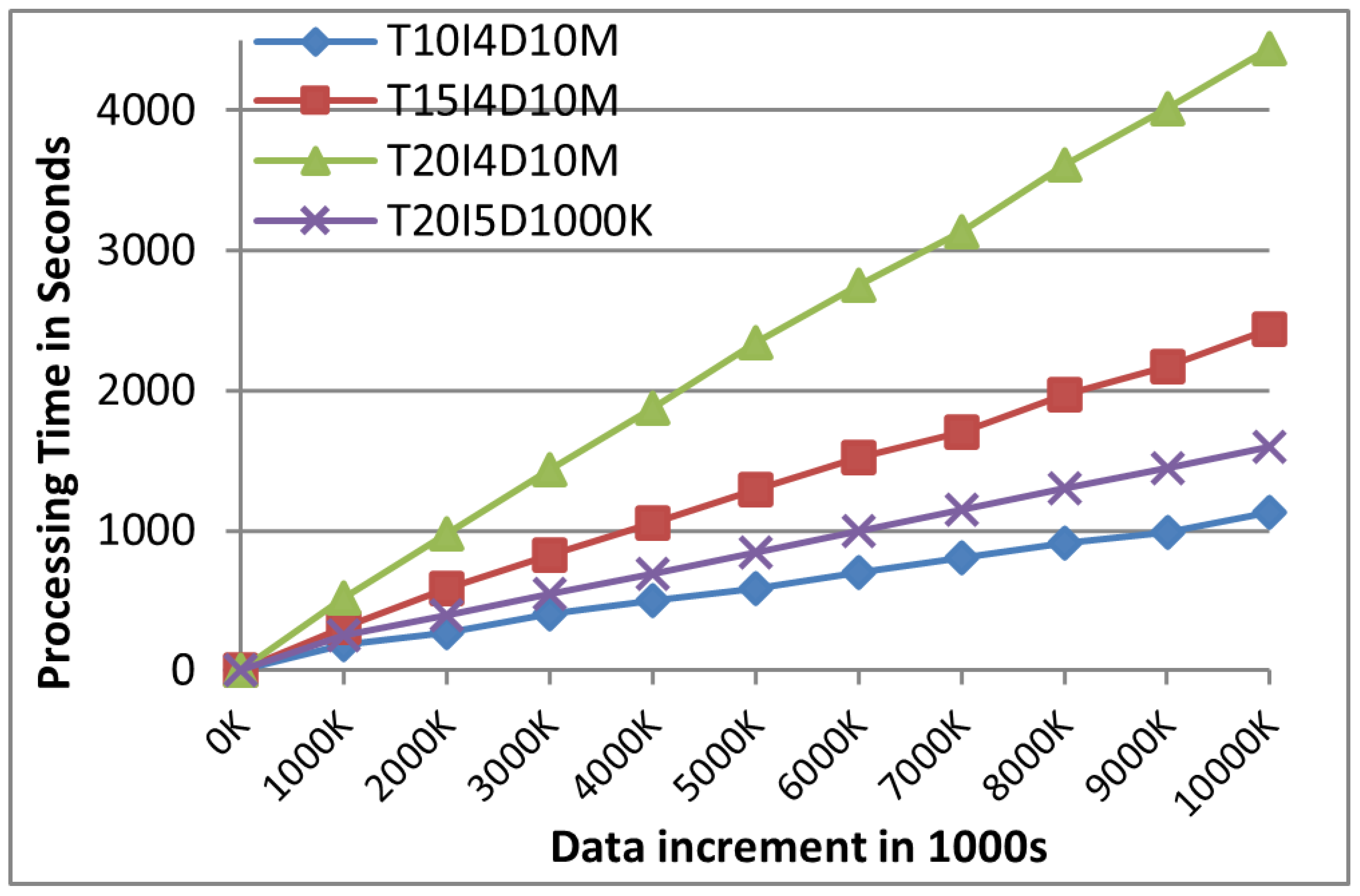
5.1. Data Scaleup

Initially, we set up processing time as a key performance indicator in comparison with a traditional distributed non-incremental FIM algorithm. As anticipated, the processing time of both algorithms exhibited a direct correlation with the size of the data increment. Figure 10 demonstrates that the non-incremental FIM algorithm showed linear growth as data kept on increasing. This basically indicates the drawback and possible inefficiency of non-incremental algorithms. Figure 10 shows the execution of the Frequent Itemset Mining against the time consumed in non-increamental data cleanup setup. It is a reflection that non-incremental FIM may not be productive in analytics of ever-increasing data, thereby making handling data more complex. 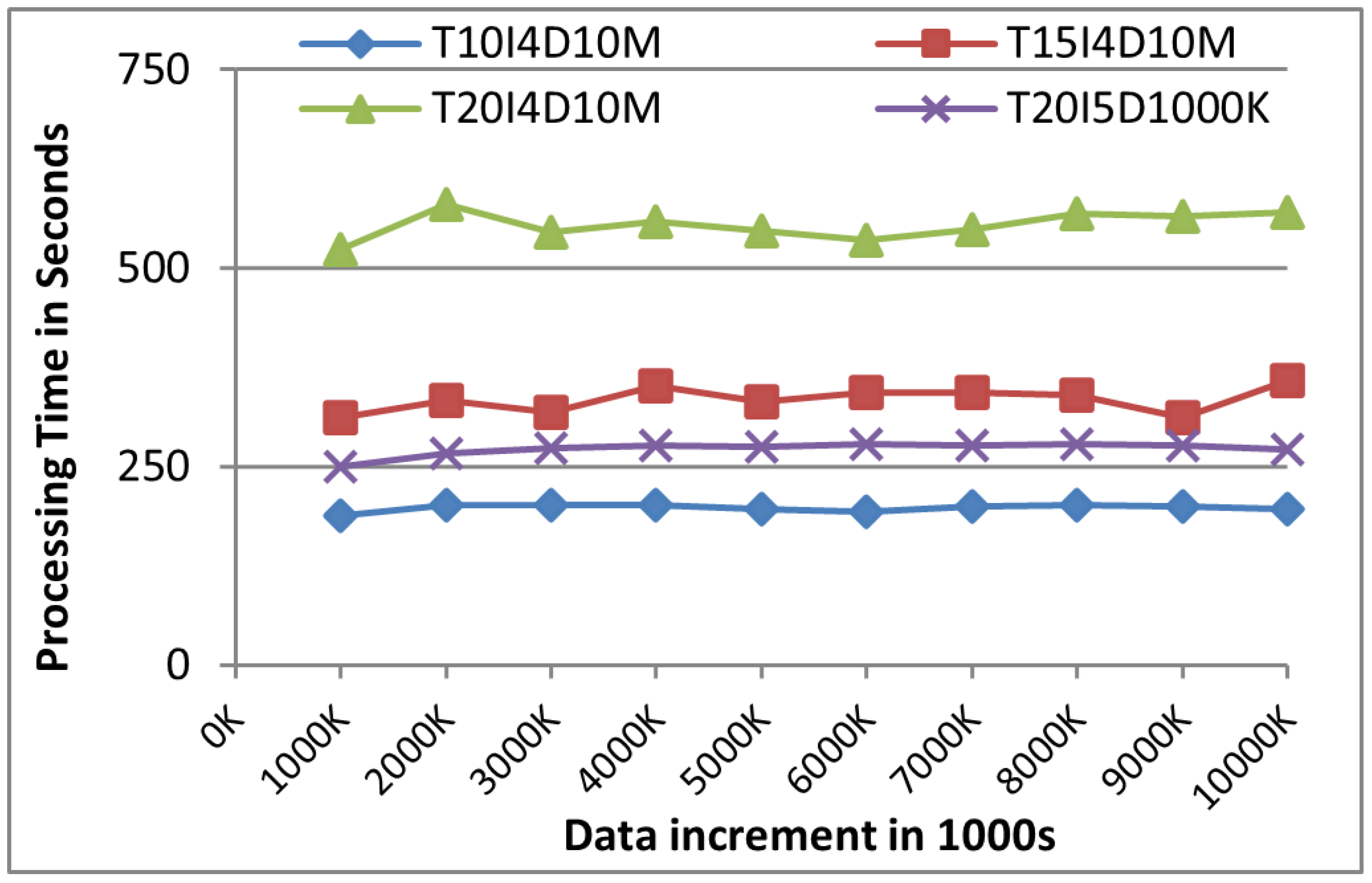In contrast, as shown in Figure 11, DIAFIM’s processing time remained relatively stable even as the dataset size increased. This performance stability can be attributed to DIAFIM’s incremental mining approach, which avoids the need to reprocess the entire dataset for each increment, resulting in significantly reduced computational overhead.

5.2. MapReduce Node Scaleup

In a distributed computing environment with an increase in the number of nodes, the performance metrics showed improved results of speed and efficiency in terms of execution time. To assess this, we conducted experiments using two datasets, each containing 1 million transactions but with varying average transaction lengths. As shown in Figure 12, the processing time decreased consistently with the addition of more nodes. Moreover, Figure 12 illustrates the speedup achieved, which demonstrates an almost linear increase in performance as the number of nodes in the cluster grows, highlighting the scalability and efficiency of the proposed algorithm in a distributed MapReduce environment.

5.3. Incremental Speedup

Figure shows that the incremental FIM algorithm speeds up the data mining process over a dataset as compared to the time taken by the traditional distributed non-incremental FIM algorithm. From the experimental results observed in Figure 13, it can be inferred that the speedup of the proposed algorithm is directly proportional to the size of the old dataset (D) and is inversely proportional to the size of the newly generated incremental dataset ($\Delta D$). Note that the incremental speedup percentage is in relation to the traditional distributed non-incremental FIM algorithm performed again and again on the entire dataset. In this experiment, the size of the incremental dataset ($\Delta D$) increased constantly by 1 million transactions.

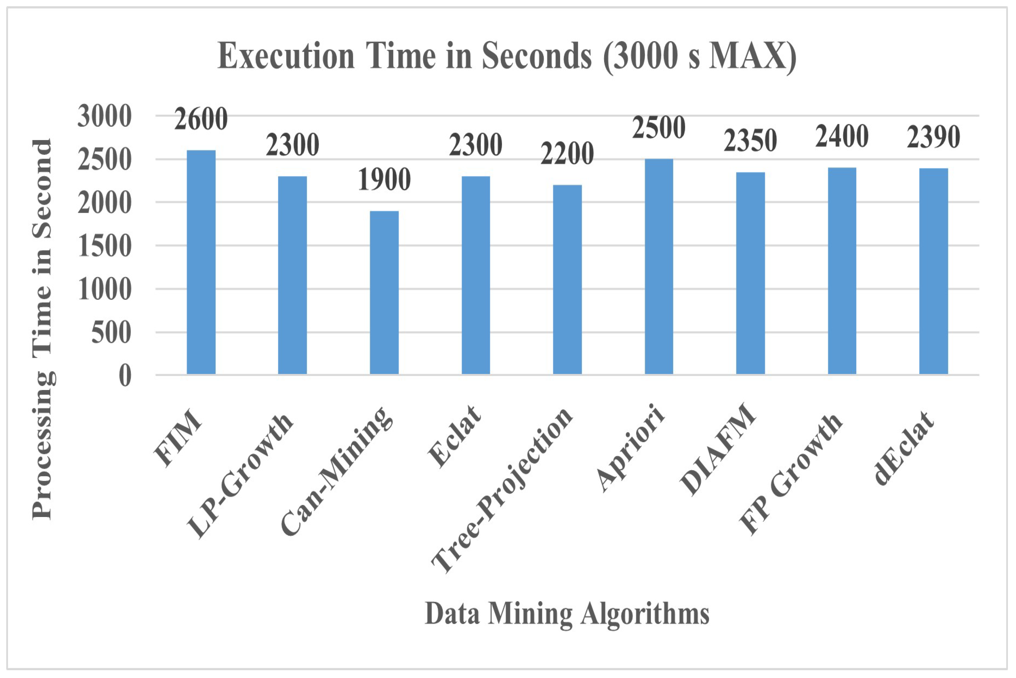
6. Comparative Analysis with Other FIM-Based Algorithms

In the research literature of data mining, frequent itemset mining algorithms are classified into three main categories, i.e., namely join-based, tree-based, and pattern-growth, as shown in Figure 14. Join-based algorithms follow the bottom–up approach for mining frequent itemsets and expand them into larger itemsets within the bounds of certain thresholds. Tree-based algorithms utilize the methodology of enumeration to identify frequent itemsets by constructing lexicographic tree. Systems can adopt either the depth-first or breadth-first search technique to extract appearing frequently.

The pattern growth algorithm adopts the MapReduce-based framework that is aimed at using the divide–conquer approach to partition the large data, determine the frequent itemsets based on certain rules, and then expand them into larger well-identified, rule-based itemsets.

Figure 14 shows a diagrammatic view of different types of algorithms. However, our focus and context of study is to develop a comparative analysis of MapReduce-based algorithms potentially dealing with large and incremental datasets. We further elaborate each of algorithm as follows.

Table 3. Analysis of the data mining algorithm.

FPM Algorithm	Methodology	Applications
FP-Growth ([47])	Preserves the association information of all itemsets; divides the data incrementally to ensure convenient search	Main theme of this itemset mining technique was market basket analysis and stock prices
LP-Growth ([48])	Generates LP-tree in a faster manner; array operations are used to develop tree based data structure across the multiple nodes	Introduces tree-based structures when data are evolving, mainly in the business domain and social media (Company Stocks, Facebook, Youtube, etc.)
CAN-Mining ([49])	An effective methodology when support values for rule-mining are set to be quite high	Outperforms the FP-Growth by time and cost
Eclat ([50])	An algorithm that queries the database to find frequent itemsets with support values	Alternative of Apriori with the design of tree-based structures for datasets
dEclat ([51])	An improved form of the Eclat algorithm that keeps track of transaction ids	Reduced running time and memory usage
Tree-Projection ([52])	Divides the large datasets into subsets and frequently occurring itemsets with tree-based search and minimum support	It was the primary attempt to organize the variety, velocity and volume of data into tree structures to extract meaningful information
Apriori ([19])	Iteratively scans the datasets of size K to develop the frequent itemset of size K + 1	Rule-based mining and association among the items to generate relavent itemmsets in big data.

provides a comprehensive analysis of extensively studied data mining algorithms in the research literature. It can be seen that new algorithms have been improved over the years as data scalability has come into effect. Moreover, updated algorithms have somehow improved the performance of the data analytics process and facilitated the process of mining data cost effectively.

Performance Evaluation

Figure 15 and Figure 16 show a comparative analysis of DIAFM with competitive algorithms in controlled distributed environment settings of 1 million transactions.

It can be well observed that DIAFM takes 2350 s, which puts it in the middle range of executions. Thus, it is efficient to process 1 million transactions. It competitively performed well in comparison to foundational algorithms such as FIM (2600 s) and Apriori (2500 s) that significantly depend on the density of the dataset, which affects scalability, because these algorithms are based on exhaustive searches. DIAFM, on the other hand, focuses on processing incremental data, thus reducing overhead from the repeated scanning of entire datasets. This renders it more appropriate for dynamic contexts in which fresh data streams are perpetually available. Although the sharding mechanism of DIAFM alleviates memory bottlenecks, it concurrently regulates shard dimensions to prevent excessive computational demands on single map nodes. DIAFM demonstrates a performance that is only slightly inferior to that of Eclat (2300 s) and Tree-Projection (2200 s), both of which are specifically optimized for dense datasets. FP-Growth, a well-established and widely used algorithm, has an execution time of 2400 ms, which is slightly higher than DIAFM. While FP-Growth excels in managing large datasets, it lacks the incremental processing advantage of DIAFM, which reduces overhead. dEclat, known for its depth-first traversal approach in itemset mining, records an execution time of 2390 ms, which is closer to FP-Growth but still higher than DIAFM. The slightly higher execution time can be attributed to dEclat’s focus on compact data representation rather than incremental updates. This suggests that DIAFM effectively accommodates both dense and sparse data distributions. DIAFM (2350 s) is much slower compared to Can-Mining (1900 s), which uses optimal techniques for frequent pattern mining. This implies that for DIAFM, the computation overhead in processing the initial shards or merging results could potentially be higher. The performance of DIAFM depends highly on shard size. Larger shards increase memory use, while smaller shards result in too many MapReduce tasks. Keeping step-by-step profile updates as well as error bounds raises the complexity of the algorithm, affecting its speed compared to simpler algorithms.

Based on the given data, the memory usage for the different algorithms of data mining (8 GB maximum capacity) and comparision among them is shown in Figure 16. It is required to infer an in-depth analysis in the manuscript context and trade-offs. Can-Mining (4.45 GB) and Tree-Projection (4.42 GB) are the most lightweight, using the least amount of memory. This may perhaps be one of the reasons why they have very lightweight computational overhead and do not use complex data structures. Can-Mining (4.45 GB) and Tree-Projection (4.42 GB) show the lowest memory consumption. Therefore, they are considered to be the most memory-saving algorithms. This may be due to their significantly lesser computations and exclusion of complex data structures. Algorithms like FIM (5.97 GB), Eclat (5.8 GB), and Apriori (5.91 GB) use significantly more memory. They work on frequent itemset storage, recursive tree building, or have high intermediate storage, respectively. The memory usage of FP-Growth has been slightly higher at 4.84 GB compared with DIAFM. Such additional memory usage is found as part of construction and maintaining its FP-Tree structure, with the need to handle various prefix trees in frequent itemset generation. dEclat has a memory usage of 5.4 GB and demands the most memory of the three. It is based on vertical data structures, where the dataset size can cause a large growth, especially on dense datasets with overlapping itemsets. DIAFM uses a memory of 4.8 GB, making it the most memory-efficient among many algorithms. This efficiency speaks for its ability to process large datasets without much memory overhead, owing to its sharding technique and incremental updates. The design of DIAFM, which effectively partitions and shuffles data, explains its balanced memory usage and speed. Unlike Apriori and FIM, it minimizes large intermediate results, and unlike Tree-Projection, it retains scalability for denser or larger datasets.

7. Discussion

Approximation strategy in frequent itemset mining based on the DIAFM method of application maintains at the same time a balance to computation efficiency and accuracy. Nevertheless, computational burdens decrease because computation is shard-based. Again, there is a cost that may be considered: when small sizes are used, this increased the inaccuracy level for those shards compared to the overall support results. In the past, several data mining techniques utilized approximation techniques with possible bottlenecks in handling large data, unmanaged complexity, and without computational error consideration [53,54].

For example, for a shard size of 10,000 transactions, the execution time decreases by about 35%, while the accuracy only by 2%. However, as the shard size increases, the errors that occur in the global support calculation become less frequent due to the better representation of the dataset; however, this benefit attracts the cost of increased memory usage and longer processing times. It reveals that shard sizes need to be optimized in both performance and accuracy based on the specific dataset and limitations of existing resources.

The DIAFM avoids exact support checks by approximating global support values using shard-level computations. This reduces the computational overhead, especially for large datasets. Although approximation introduces small inaccuracies in identifying frequent itemsets, it enables much faster execution compared to exact methods like Apriori. Shard-level error thresholds and periodic updates to global support calculations help limit inaccuracies and maintain scalability.

Traditional FIM algorithms have difficulties adapting to the fast-growing or changing nature of the datasets, normally requiring the full dataset to be rescanned. The incremental process of DIAFM execution is only effective over the new data, thereby reducing computational requirements by orders of magnitude, and therefore, making the updates faster. By combining approximation with incremental updates, DIAFM provides a practical solution to frequent itemset mining in dynamic, large-scale scenarios.

8. Conclusions

In this paper, we addressed the limitations of traditional non-incremental frequent itemset mining (FIM) algorithms, particularly their inefficiency in handling rapidly growing datasets. We proposed a novel distributed and incremental FIM algorithm, DIAFIM, utilizing the MapReduce framework, which effectively leverages the parallel and distributed nature of Hadoop. By employing MapReduce, the algorithm overcomes significant challenges related to concurrency control, fault tolerance, and network communication, ensuring scalability and robustness in distributed environments.

This paper addresses limitations in traditional non-incremental frequent itemset mining (FIM) algorithms, especially their inefficiency in handling large, dynamic datasets. The distributed incremental approximation FIM (DIAFM) algorithm thus extends these capabilities by using the concept of sharding, approximation, profile integration in MapReduce-based framework for scalability, robustness, and fault tolerance in distributed settings.

We detail the key findings of our research study as follows: (1) Simplified approximation and trade-off process—DIAFM scanners scan the dataset a few times but never performs exact support checks, which results in computations that are always efficient, but degrades to lower accuracy. (2) Scalability—The algorithm demonstrates efficient performance with the increase in dataset size and computational nodes. (3) Incremental Processin—It processes only new data increments, which significantly reduces execution time compared to traditional methods. (4) Comparative Competitiveness—Benchmarks show that DIAFM performs competitively with established FIM algorithms in terms of both execution time and memory usage.

It is evident that this research is the introduction of an efficient approximation method that avoids the need for multiple dataset scans and eliminates the additional step of checking the exact support of itemsets. This approach enhances the performance of FIM in large-scale datasets while maintaining an acceptable trade-off between accuracy and computational efficiency. DIAFIM’s incremental design ensures that only new data increments are processed, significantly reducing processing time compared to traditional methods. Our results demonstrate that DIAFIM scales efficiently with growing datasets and an increasing number of computational nodes, offering a practical solution for mining frequent itemsets in dynamic, distributed environments.

While DIAFM shows stable performance for moderately large datasets, its sharding mechanism and data distribution strategies may face bottlenecks when dealing with ultra-massive datasets that require distributed environments with thousands of nodes. Fine-tuning for such extreme scalability may be necessary. The chosen sharding strategy plays a major role in the efficiency of DIAFM. Poorly optimized sharding can lead to an imbalanced workload distribution and increased computational overhead. This limitation requires further investigation into automatic sharding techniques to optimize performance across diverse datasets. Although incremental updates save some recomputation, they add some overhead of computation, mainly when updates are very frequent and abundant. This might adversely affect the performance of the algorithm in highly dynamic scenarios. The study mainly compares DIAFM with the traditional frequent itemset mining algorithms. However, the emergence of deep learning-based methods in association rule mining may also be used to further provide insights into how DIAFM performs against advanced approaches. Future work may investigate these comparisons to establish wider applicability. DIAFM’s performance may depend on dataset characteristics such as density, sparsity, and dimensionality.

Although the present evaluation proves its robustness, further study is needed to determine how well it adapts to highly sparse or highly dense datasets. These limitations open avenues for future research to further optimize DIAFM’s scalability and its sharding mechanisms, and to expand its applicability to more challenging data mining problems. In doing so, DIAFM can further solidify its position as a robust and scalable solution for frequent itemset mining in diverse applications. DIAFM’s design is well suited to modern data analytics domains that include, for example, real-time transaction analysis, social network mining, and IoT data streams, among others, offering a practical and scalable solution for frequent itemset mining in dynamic, distributed settings.

These contributions address some of the key challenges in frequent itemset mining and offer an efficient and scalable alternative to traditional methods. DIAFM introduces shard-based processing, approximation techniques, and incremental updates to ensure robust performance on a variety of datasets and computing environments. In addition to its technical contributions, DIAFM has a strong aptitude for practical applications in many modern data-intensive domains. As an example, it is quite applicable in real-time transaction analysis, social network mining, IoT data streams, and e-commerce recommendation systems. These domains often require frequent updates, scalable solutions to handle dynamic datasets, and distributed datasets. The incremental design and efficient approximation of this algorithm make it particularly more suitable for these use cases.

Further research could involve optimizations at the shard level, adaptive shard sizing with characteristics of the datasets, and integration into newly emerging distributed computing frameworks to improve the performance and usability of DIAFM. All of these advancements presented in this paper pave the way for scalable and efficient frequent itemset mining in a world of increasingly complex and dynamic data landscapes.