Solution of Fractional Differential Boundary Value Problems with Arbitrary Values of Derivative Orders for Time Series Analysis

Abstract

The paper considers the solution of a fractional differential boundary value problem, that is, a diffusion-type equation with arbitrary values of the derivative orders on an infinite axis. The difference between the obtained results and other authors’ ones is that these involve arbitrary values of the derivative orders. The solutions described in the literature, as a rule, are considered in the case when the fractional time derivative β lies in the range: 0 < β ≤ 1, and the fractional state derivative α (the variable describing the state of the process) is in the range: 1 < α ≤ 2. The solution presented in the article allows us to consider any ranges for α and β, if the inequality 0 < β/α ≤ 0.865 is satisfied in the range β/α. In order to solve the boundary value problem, the probability density function of the observed state x of a certain process (for example, the magnitude of the deviation of the levels of a time series) from time t (for example, the time interval for calculating the amplitudes of the deviation of the levels of a time series) can be captured.

1. Introduction

Complex systems can be defined as structures in which at least one element is a human. On the one hand, the action of many random factors leads to the stochastic properties of such systems. In addition to stochasticity, uncertainty also arises, associated in some cases with the irrationality of human behavior. On the other hand, the presence of the human factor creates prerequisites for the self-organization of such systems and can determine the existence of memory of their previous states. All this leads to the appearance of organized complexity (emergence).

This cannot be considered as the result of a simple summation of the characteristics of the elements, but rather the result of the emergence of systemic connections and adaptive redistribution of functions between the elements. It should be noted that the models for describing most of the processes observed in complex social and economic systems can be classified as non-stationary time series.

Due to the nonlinearity and variability of the characteristics of processes occurring in complex social and economic systems, traditional methods of analyzing and modeling their time series, such as the integrated autoregressive moving average model (ARIMA, Box–Jenkins model) and many other models, often lead to inaccurate or erroneous results.

The use of differential equations of various types for the analysis and modeling of the dynamics of economic and social processes, as well as for forecasting the evolution of states in social and economic systems, is very important and is widely used. For example, the Fokker–Planck equation and its analogues are often used in the analysis of time series of financial and commodity market indices, currency pair ratios, and much more. In this regard, one can, for example, mention the well-known Black–Scholes efficient market model.

However, the approaches currently used for this, including neural network models, for example, for solving problems of regression restoration, although showing good results in a number of cases, do not consider the possibility of self-organization in complex systems and the presence of memory but are limited to considering Markov processes. In this regard, in our opinion, it is more acceptable to create models for analyzing and describing the dynamics of processes in complex systems based on fractional differential equations in partial derivatives. Fractional equations, both in terms of time and the variable describing changes in the time series, can be used to account for memory effects and the possibility of self-organization.

The fractional nature of the derivatives of operators with respect to time and the variable determining the level of the series makes it possible to describe non-local processes in which the transition to a given state of the system (or process) depends not only on the local characteristics of the process or the behavior of the system in the vicinity of the point under consideration, but also on the values it takes on the entire range of values (i.e., memory) under consideration, and non-locality with respect to time can lead to self-organization.

Currently, fractional differential models are being developed to describe the dynamics of processes in complex systems. For example, [1] discusses the development of a fractional hyperchaotic economic system of variable order with a nonlinear model predictive regulator. In the presented work, the authors develop a model of the dynamics of an economic system based on a system of four differential equations with fractional time derivatives of indicators of changes in system characteristics.

The results of the model analysis show that the presented approach not only allows the suppression of the chaotic behavior of the parameters describing the system and stabilization of the closed system, but also the rejection of limited external perturbations.

In [2] is described the use of Mittag–Leffler fractional integrals (ML) to solve a system of two related fractional stochastic differential equations. The fractional stochastic process, according to the author, can be described through the fractional stochastic integral relative to the standard Brownian motion, and the studied processes are Gaussian, not Markov, processes, with the property of a long-acting dependence, which allows for considering memory. Thanks to the obtained solutions for covariance of such processes, the author [2] developed algorithms for modeling neural dynamics.

Unfortunately, this article only considers the solution of a system of two fractional differential equations for the case when the value of the orders of fractional derivatives does not exceed 1, which somewhat limits the scope of the resulting model.

Solutions of fractional differential equations described in the literature are usually considered when the value of the value of the fractional time derivative $\beta$ is in the range: $0<\beta \le 1$, and the fractional derivative by state $\alpha$ (variable describing the state of the process) is in the range: $1<\alpha \le 2$, which limits the use of fractional differential models for time series dynamics analysis.

The purpose of the work is to find an analytical function of the probability density of observing the amplitude of deviation of the levels of the time series depending on the time interval for calculating these amplitudes for the infinite axis based on the fractional differential equation of the diffusion type with arbitrary values of the indices of fractional derivatives.

2. Differential Equations with Fractional Partial Derivatives

A diffusion-type differential equation with fractional partial derivatives in the general case has the following form:

$${\displaystyle \frac{{\partial }^{\beta }\rho \left(x,t\right)}{\partial t^{\beta }}}=D{\displaystyle \frac{{\partial }^{\alpha }\rho \left(x,t\right)}{\partial x^{\alpha }}}$$

(1)

where $\alpha$ and $\beta$ are fractional derivative indices (according to Caputo) and positive real numbers, $\rho (x, t)$ is the probability density function of observing state $x$ at time $t$, depending on time $t$ and state $x$, and $D$ is a certain constant coefficient. For example, when describing diffusion, $\rho (x, t)$ plays the role of the concentration of the diffusing substance, and $D$ is the diffusion coefficient.

In general, the fractional derivative of order ν for a function $\psi \left(x\right)$ is defined as follows [3]:

$${\displaystyle \frac{d^{\nu }\psi \left(x\right)}{d{x}^{\nu }}}={\displaystyle \frac{1}{\mathrm{\Gamma }(1-\left[\nu \right])}}·{\displaystyle \frac{d^{⌈v⌉}}{d{x}^{⌈v⌉}}}{\int }_a^x{\displaystyle \frac{f\left(\xi \right)d\xi }{{\left\{x-\xi \right\}}^{⟦v⟧}}}$$

where $⟦v⟧<1$ is the fractional part of the exponent ν, and $⌈v⌉$ is the rounding of the fractional exponent ν to the nearest largest integer value, i.e., $⟦v⟧=v+1-⌈v⌉$.

The Caputo definition of fractional derivatives differs from the Riemann–Liouville definition in that the function is first differentiated to integer order $n$, greater than the non-integer order after rounding to an integer ($⌈v⌉$), and then the result is integrated to order $1-⟦v⟧$.

At present, an analytical solution of the fractional diffusion Equation (1) has been obtained only for the case $0<\beta \le 1$ and $1\le \alpha \le 2$; see [4,5,6,7,8,9,10,11]. Solutions outside the boundaries of the specified values of $\alpha$ and $\beta$ are not presented in the literature.

When solving practical issues related to the analysis and forecasting of the dynamics of time series for complex processes, it may turn out that the condition $0<\beta \le 1$ and $1\le \alpha \le 2$ is a limitation of the model, and the values of $\alpha$ and $\beta$ may go beyond the specified ranges.

Due to the complexity of the problems to be solved and the significant difficulties in obtaining analytical solutions, numerical methods are very often used in practice. For example, in the work [12], using numerical methods, the solution of an equation of the form was investigated for a segment:

$${\displaystyle \frac{\rho \left(x,t\right)}{\partial t}}=D{\displaystyle \frac{{\partial }^{\alpha }\rho \left(x,t\right)}{\partial x^{\alpha }}} \mathrm{for} 1<\alpha <2$$

And in the work [13], the solution for a segment of an equation of the form:

$${\displaystyle \frac{{\partial }^{\beta }\rho \left(x,t\right)}{\partial t^{\beta }}}=D{\displaystyle \frac{{\partial }^2\rho \left(x,t\right)}{\partial x^2}} \mathrm{for} 0<\mathsf{\beta }\le 1$$

It is interesting to compare the fractional differential Equation (1) with the equation of ordinary diffusion: ${\displaystyle \frac{\partial \rho \left(x,t\right)}{\partial t}}=D{\displaystyle \frac{{\partial }^2\rho \left(x,t\right)}{\partial x^2}}$, the solution of which on the infinite axis allows us to obtain the Poisson distribution law:

$$\rho \left(x,t\right)={\displaystyle \frac{1}{2\sqrt{\pi \mathrm{D}t}}}{·e}^{-{\displaystyle \frac{x^2}{4·D·t}}}$$

The function $\rho (x, t)$ for example, can be interpreted as the probability density of observing some value of the level of the time series at time $t$, if these levels can randomly change over time.

In case of Poisson distribution, the dispersion ${\sigma }^2\left(t\right)$ will have a linear law of its dependence on time (${\sigma }^2\left(t\right)~t$)). If there is a slower growth ${\sigma }^2\left(t\right)$ from $t$ (${\sigma }^2\left(t\right)~\sqrt[\beta ]{t}$, where $0<\beta <1$), then such a process is qualified as subdiffusion [14,15]; if there is a faster growth ${\sigma }^2\left(t\right)$ from t (${\sigma }^2\left(t\right)~t^{\beta }$, where $1<\beta <2$), then such a process is qualified as superdiffusion [16]. The distribution function describing subdiffusion type processes is obtained from the solution of a fractional differential equation of the form: ${\displaystyle \frac{{\partial }^{\beta }\rho \left(x,t\right)}{\partial t^{\beta }}}=D{\displaystyle \frac{{\partial }^2\rho \left(x,t\right)}{\partial x^2}}$, and superdiffusion from the equation, ${\displaystyle \frac{\partial \rho \left(x,t\right)}{\partial t}}=D{\displaystyle \frac{{\partial }^{\alpha }\rho \left(x,t\right)}{\partial x^{\alpha }}}$, where $\alpha$ and $\beta$ are the exponents of fractional derivatives, and $D$ is a certain coefficient (for example, the diffusion coefficient). Anomalous diffusion processes can also be observed [17,18] described by a fractional differential equation of mixed type (see Equation (1)).

In addition to the fractional diffusion equation, other types of fractional differential equations are of considerable interest. For example, in [19,20,21,22,23], the solution of the fractional Zener wave equation is considered:

$${\nabla }^2\mathcal{U}\left(x,y,z,t\right)-{\displaystyle \frac{1}{c_0^2}}{\displaystyle \frac{{\partial }^2\mathcal{U}\left(x,y,z,t\right)}{\partial t^2}}+{\tau }_{\sigma }^{\alpha }{\displaystyle \frac{{\partial }^{\alpha }}{\partial t^{\alpha }}}{\nabla }^2\mathcal{U}\left(x,y,z,t\right)-{\displaystyle \frac{{\tau }_{ϵ}^{\beta }}{c_0^2}}{\displaystyle \frac{{\partial }^{\beta +2}\mathcal{U}\left(x,y,z,t\right)}{\partial t^{\beta +2}}}=0$$

where $\mathcal{U}\left(x,y,z,t\right)$ in the case of elastic waves is the displacement of the particles of the medium from the equilibrium position at the point with coordinates $x,y,z$ at time $t$; $c_0$ is the wave propagation velocity; ${\tau }_{ϵ}$ and ${\tau }_{\sigma }$ are some positive time constants. In this case, $\alpha$ and $\beta$ are different values of fractional derivatives with respect to time, and the operator ${\nabla }^2$ is not fractional.

The Zener stress–strain relationship is utilized for elastic wave propagation, alongside the linearized conservation of mass and momentum. The Zener wave equation facilitates the description of three distinct modes of wave attenuation that exhibit power law characteristics [19]. Models derived from this equation find applications in fields such as medical elastography and acoustics.

In [21], a detailed description of the solution of the Zener equation for the case $\alpha =\beta$ ($\alpha$ and $\beta$ can be derivative fractional positive numbers that define derivatives with respect to time $t$) is presented. This result is very important, since the solution of any fractional differential equations in analytical form has significant problems.

The solution of wave equations with a fractional time derivative was further developed in [22] to describe the behavior of waves in non-Newtonian fluids.

Note that the solution of the Schrödinger equation with fractional derivatives is also of interest.

Currently, the most developed and studied are fractional differential models created to describe various types of physical problems, mainly devoted to the study of processes of physical kinetics, diffusion and relaxation in various environments [23,24,25,26,27,28,29,30], in [31] the analysis of time series of sociodynamic processes based on fractional differential equations was considered.

It should be noted that several studies [32] have developed models that describe complex processes while incorporating memory effects and self-organization, albeit without the consideration of fractional differential equations.

3. Formulation of the Boundary Value Problem

Let us consider the following problem: Let there be a differential equation with fractional derivatives of the diffusion type:

$${\displaystyle \frac{{\partial }^{\beta }\rho \left(x,t\right)}{\partial t^{\beta }}}=D{\displaystyle \frac{{\partial }^{\alpha }\rho \left(x,t\right)}{\partial x^{\alpha }}}$$

where $\rho (x,t)$ is the probability density function of observing the state $x$ of some process (for example, the magnitude of the deviation of the levels of a time series) from time $t$ (for example, the time interval for calculating the amplitudes of the deviation of the levels of a time series), $D$ is a certain constant coefficient, and $\mathsf{\alpha }$ and $\mathsf{\beta }$ are the indices of the fractional derivative ($0<\mathsf{\beta }$ and $0<\mathsf{\alpha }$). Note that the values of $\mathsf{\alpha }$ and $\mathsf{\beta }$ do not necessarily have to lie, as is usually considered in other studies, in the ranges $1<\alpha <2$ and $0<\beta <1$.

Using the following boundary conditions:

$${\left.\rho (x,t)\right|}_{\mathrm{x}\to -\mathrm{\infty }}={\left.\rho (x,t)\right|}_{\mathrm{x}\to \mathrm{\infty }}=0$$

and the initial condition:

$$\rho \left(x,0\right)=\delta \left(x-0\right)$$

let us consider the boundary value problem of finding the function $\rho (x,t)$ for the given conditions with arbitrary positive real values of $\mathsf{\alpha }$ and $\mathsf{\beta }$.

4. Solution of the Boundary Value Problem

Let us perform the Laplace transform for Equation (1) with respect to t (we move from t to s) and the Fourier transform with respect to x (we move from x to k), which allows us to obtain a double image $\widetilde{\overline{G\left(k,s\right)}}$ for the function $\rho (x,t)$:

$$s^{\beta }\overline{G\left(x,s\right)}-{\displaystyle \frac{\rho \left(x,0\right)}{s^{1-\beta }}}=D{\displaystyle \frac{d^{\alpha }\overline{G\left(x,s\right)}}{d{x}^{\alpha }}}$$

You can find detailed information about Laplace transformations of franctional derivatives in the book [18]. The following is the Fourier transform:

$$\underset{-\mathrm{\infty }}{\overset{+\mathrm{\infty }}{\int }}{\displaystyle \frac{d^{\alpha }\overline{G\left(x,s\right)}}{d{x}^{\alpha }}}·{\mathrm{e}}^{ixk}dx={\left(ik\right)}^{\mathsf{\alpha }}·\widetilde{\overline{G\left(k,s\right)}}$$

$$\widetilde{\rho \left(k,0\right)=}\underset{-\mathrm{\infty }}{\overset{+\mathrm{\infty }}{\int }}\rho \left(x,0\right)·{\mathrm{e}}^{ixk}dx=\underset{-\mathrm{\infty }}{\overset{+\mathrm{\infty }}{\int }}\delta \left(x-0\right)·{\mathrm{e}}^{ixk}dx=1$$

$$\widetilde{\overline{G\left(k,s\right)}}=\underset{-\mathrm{\infty }}{\overset{+\mathrm{\infty }}{\int }}\overline{G\left(x,s\right)}·{\mathrm{e}}^{ixk}dx$$

Substituting Fourier images into the equation obtained after the Laplace transform, we write the following:

$$s^{\beta }·\widetilde{\overline{G\left(k,s\right)}}-{\displaystyle \frac{1}{s^{1-\beta }}}={\left(ik\right)}^{\alpha }D·\widetilde{\overline{G\left(k,s\right)}}$$

Then we obtain the following:

$$\widetilde{\overline{G\left(k,s\right)}}={\displaystyle \frac{1}{s^{1-\beta }·\left\{s^{\beta }-{\left(ik\right)}^{\alpha }D\right\}}}={\displaystyle \frac{1}{s·\left\{1-\frac{{\left(ik\right)}^{\alpha }D}{s^{\beta }}\right\}}}$$

(2)

Let us denote $\nu =\left|{\displaystyle \frac{{\left(ik\right)}^{\alpha }D}{s^{\beta }}}\right|$ and, taking ($0\le \nu <1$), we carry out the binomial expansion:

$$\widetilde{\overline{G\left(k,s\right)}}={\displaystyle \frac{1}{s\left\{1-\frac{{\left(ik\right)}^{\mathsf{\alpha }}D}{s^{\beta }}\right\}}}={\displaystyle \frac{1}{s\left\{1-\nu \right\}}}={\displaystyle \frac{1}{s}}\sum _{q=0}^{\mathrm{\infty }}{\nu }^q={\displaystyle \frac{1}{s}}\sum _{q=0}^{\mathrm{\infty }}{\left\{{\displaystyle \frac{{\left(ik\right)}^{\mathsf{\alpha }}D}{s^{\beta }}}\right\}}^q=\sum _{q=0}^{\mathrm{\infty }}{\displaystyle \frac{{\left\{{\left(ik\right)}^{\mathsf{\alpha }}D\right\}}^q}{s^{\beta q+1}}}$$

Next, we perform the inverse Laplace transform and move from the image s to the original $t$:

$$\widetilde{G\left(k,t\right)}=\sum _{q=0}^{\mathrm{\infty }}{\displaystyle \frac{{\left\{{\left(ik\right)}^{\mathsf{\alpha }}·D{t}^{\mathsf{\beta }}\right\}}^q}{\mathrm{\Gamma }\left(\mathsf{\beta }q+1\right)}}$$

(3)

According to the tables, for inverse Laplace transforms:

$${\displaystyle \frac{1}{s^{\beta q+1}}}:={\displaystyle \frac{t^{\beta q}}{\mathrm{\Gamma }\left(\mathsf{\beta }q+1\right)}}$$

Note that $\widetilde{G\left(k,t\right)}$ is the Mittag–Leffler function. To perform the inverse Fourier transform of this function and find the distribution density, we move from calculating the infinite sum to the integral representation of the Mittag–Leffler function through the contour integral [33]. For this, we use the Hankel representation for the Euler gamma function:

$${\displaystyle \frac{1}{\mathrm{\Gamma }\left(\tau \right)}}={\displaystyle \frac{1}{2\pi i}}\underset{{\mathit{C}}^{\prime }}{\int }{e}^u{u}^{-\tau }du=-{\displaystyle \frac{1}{2\pi i}}\underset{{\mathit{C}}^{″}}{\int }{e}^{-u}{(-u)}^{-\tau }du$$

where ${\mathit{C}}^{\prime }$ is the integration contour that starts from $–\infty$, reaches $0$, goes around it counterclockwise, and returns back, and ${\mathit{C}}^{″}$ is the integration contour that starts from $+\infty$, reaches $0$, goes around the point $0$ counterclockwise, and returns back. Using this representation of the gamma function and the contour, ${\mathit{C}}^{″}$ we obtain the following:

$$\begin{gathered} \widetilde{G\left(k,t\right)}=\sum _{q=0}^{\mathrm{\infty }}{\displaystyle \frac{{\left\{{\left(ik\right)}^{\mathsf{\alpha }}·D{t}^{\mathsf{\beta }}\right\}}^q}{\mathrm{\Gamma }\left(\mathsf{\beta }q+1\right)}}=\sum _{q=0}^{\mathrm{\infty }}{\displaystyle \frac{{\xi }^q}{\mathrm{\Gamma }\left(\beta q+1\right)}}=-{\displaystyle \frac{1}{2\pi i}}\sum _{q=0}^{\mathrm{\infty }}{\left\{{\left(ik\right)}^{\mathsf{\alpha }}·D{t}^{\mathsf{\beta }}\right\}}^q\underset{{\mathit{C}}^{″}}{\int }{e}^{-u}·{\left(-u\right)}^{-\beta q-1}du \\ =-{\displaystyle \frac{1}{2\pi i}}\underset{{\mathit{C}}^{″}}{\int }{\displaystyle \frac{e^{-u}{·(-u)}^{\beta -1}}{{(-u)}^{\beta }-\left\{{\left(ik\right)}^{\mathsf{\alpha }}·D{t}^{\mathsf{\beta }}\right\}}}du \end{gathered}$$

(4)

Let us perform the inverse Fourier transform of the function ${\displaystyle \frac{e^{-u}{·(-u)}^{\beta -1}}{{(-u)}^{\beta }-\left\{{\left(ik\right)}^{\alpha }·D{t}^{\beta }\right\}}}$:

$${\displaystyle \frac{1}{2\pi }}\underset{-\mathrm{\infty }}{\overset{\mathrm{\infty }}{\int }}{\displaystyle \frac{e^{-u}{·(-u)}^{\beta -1}·e^{-ik\left|x\right|}dk}{{(-u)}^{\beta }-\left\{{\left(ik\right)}^{\mathsf{\alpha }}·D{t}^{\mathsf{\beta }}\right\}}}$$

(5)

To calculate the resulting integral, we can use the theory of residues. We can consider an analytical continuation of the function ${\displaystyle \frac{e^{-ik\left|x\right|}}{{(-u)}^{\beta }-\left\{{\left(ik\right)}^{\mathsf{\alpha }}·D{t}^{\mathsf{\beta }}\right\}}}$ to the imaginary plane and go to a closed contour G, inside which the poles of the function will be located.

According to the fundamental theorem of residue theory, the integral over a chosen closed contour G will be equal to the sum of the residues at the singular points enclosed by that contour, with one side corresponding to the integral over the real axis, which must be found to solve the problem.

When finding residues, it is necessary to consider that the integrand possesses (5) a simple pole:

$$k=-i{\left\{{\displaystyle \frac{{(-u)}^{\beta }}{D{t}^{\mathsf{\beta }}}}\right\}}^{1/\alpha }$$

Note that for $k=0$:

$$\widetilde{G\left(0,t\right)}=-{\displaystyle \frac{1}{2\pi i}}\underset{{\mathit{C}}^{″}}{\int }{\displaystyle \frac{e^{-u}{·\left(-u\right)}^{\beta -1}}{{\left(-u\right)}^{\beta }}}du=-{\displaystyle \frac{1}{2\pi i}}\underset{{\mathit{C}}^{″}}{\int }{e}^{-u}{·\left(-u\right)}^{-1}du={\displaystyle \frac{1}{\mathrm{\Gamma }\left(1\right)}}=1$$

Thus, the function $\widetilde{G\left(k,t\right)}$ meets the normalization conditions and can be considered as a probability density function of some distribution.

The contour integral can be represented as the sum of the integrals over the corresponding sides of the contour. The integral that must be computed to obtain the inverse Fourier transform is determined by the side of the contour lying on the real axis.

The whole contour will consist of the side lying on the real axis (the integral that we need to calculate), the arc of the circle (radius R→∞), integration over which will give 0, and the beam (denote it $\gamma \left(ϴ\right)$), integral over which is equal to

$$\begin{gathered} \underset{\mathit{\gamma }\left(\mathit{ϴ}\right)}{\int }{\displaystyle \frac{e^{-u}{·(-u)}^{\beta -1}}{{(-u)}^{\beta }-\left\{{\left(ik\right)}^{\alpha }·D{t}^{\beta }\right\}}}du=\underset{\mathit{R}}{\overset{\mathbf{0}}{\int }}{\displaystyle \frac{e^{-r{e}^{i\frac{2\pi }{\beta }}}{·\left(-r{e}^{i\frac{2\pi }{\beta }}\right)}^{\beta -1}·e^{i\frac{2\pi }{\beta }}}{{\left(-r{e}^{i\frac{2\pi }{\beta }}\right)}^{\beta }-\left\{{\left(ik\right)}^{\alpha }·D{t}^{\beta }\right\}}}dr \\ =\underset{\mathit{R}}{\overset{\mathbf{0}}{\int }}{\displaystyle \frac{e^{-r{e}^{i\frac{2\pi }{\beta }}}{·\left(-r\right)}^{\beta -1}}{{\left(-r\right)}^{\beta }-\left\{{\left(ik\right)}^{\alpha }·D{t}^{\beta }\right\}}}dr \\ =-\underset{R\to \mathrm{\infty }}{\mathrm{l}\mathrm{i}\mathrm{m}}\underset{0}{\overset{\mathrm{\infty }}{\int }}{\displaystyle \frac{e^{-r{e}^{i\frac{2\pi }{\beta }}}{·\left(-r\right)}^{\beta -1}}{{\left(-r\right)}^{\beta }-\left\{{\left(ik\right)}^{\alpha }·D{t}^{\beta }\right\}}}dr \end{gathered}$$

A replacement was made here: $\gamma \left(ϴ\right):\left\{\begin{array}{c}y=r{e}^{i{\displaystyle \frac{2\pi }{\beta }}} \\ 0\le {\displaystyle \frac{2\pi }{\beta }}\le 2\pi \end{array}\right.$

Obviously, this approach does not give the desired result.

In order to try to obtain a solution, we formulated the hypothesis that the integral ${\int }_{-\mathrm{\infty }}^{\mathrm{\infty }}{\displaystyle \frac{e^{-u}{·(-u)}^{\beta -1}·e^{-ik\left|x\right|}dk}{{(-u)}^{\beta }-\left\{{\left(ik\right)}^{\mathsf{\alpha }}·D{t}^{\mathsf{\beta }}\right\}}}$, if it is represented through the sum of the integrals on the sides of the contour, is equal to the sum of the residues covered by the contour multiplied by some constant (C), which appears due to the fact that the integral over the beam can be expressed through the integral over the side of the contour lying on the real axis.

Note that

$$\underset{0}{\overset{\mathrm{\infty }}{\int }}{\displaystyle \frac{e^{-r{e}^{i\frac{2\pi }{\beta }}}{·\left(-r\right)}^{\beta -1}}{{\left(-r\right)}^{\beta }-\left\{{\left(ik\right)}^{\mathsf{\alpha }}·D{t}^{\mathsf{\beta }}\right\}}}dr=\underset{0}{\overset{\mathrm{\infty }}{\int }}{\displaystyle \frac{e^{-r\left\{\cos \left(\frac{2\pi }{\beta }\right)+isin\left(\frac{2\pi }{\beta }\right)\right\}}{·\left(-r\right)}^{\beta -1}}{{\left(-r\right)}^{\beta }-\left\{{\left(ik\right)}^{\mathsf{\alpha }}·D{t}^{\mathsf{\beta }}\right\}}}dr$$

$$\left|\underset{0}{\overset{\mathrm{\infty }}{\int }}{\displaystyle \frac{e^{-r\left\{\cos \left(\frac{2\pi }{\beta }\right)+isin\left(\frac{2\pi }{\beta }\right)\right\}}{·\left(-r\right)}^{\beta -1}}{{\left(-r\right)}^{\beta }-\left\{{\left(ik\right)}^{\mathsf{\alpha }}·D{t}^{\mathsf{\beta }}\right\}}}dr\right|\le \underset{0}{\overset{\mathrm{\infty }}{\int }}{\displaystyle \frac{e^{-r\cos \left(\frac{2\pi }{\beta }\right)}{·\left(-r\right)}^{\beta -1}}{{\left(-r\right)}^{\beta }-\left\{{\left(ik\right)}^{\mathsf{\alpha }}·D{t}^{\mathsf{\beta }}\right\}}}dr$$

Next, to find special points, write ${(-u)}^{\beta }-\left\{{\left(ik\right)}^{\mathsf{\alpha }}·D{t}^{\mathsf{\beta }}\right\}=0$. The denominator turns to 0 at $\mathrm{k}=-i{\left\{{\displaystyle \frac{{(-u)}^{\beta }}{D{t}^{\mathsf{\beta }}}}\right\}}^{1/\alpha }$; it will be a simple pole of the first order. In accordance with the theory of residues, the res will be equal:

$$\begin{gathered} 2\pi i\mathit{C}\sum _{l}res\left[{\displaystyle \frac{e^{-u}{·\left(-u\right)}^{\beta -1}·e^{-ik\left|x\right|}dk}{{\left(-u\right)}^{\beta }-\left\{{\left(ik\right)}^{\mathsf{\alpha }}·D{t}^{\mathsf{\beta }}\right\}}}\right]=-2\pi \mathit{C}{\displaystyle \frac{e^{-u}{·\left(-u\right)}^{\beta -1}·e^{-\left|x\right|{\left\{\frac{{\left(-u\right)}^{\beta }}{D{t}^{\mathsf{\beta }}}\right\}}^{1/\alpha }}}{\alpha {\left\{\frac{{\left(-u\right)}^{\beta }}{D{t}^{\mathsf{\beta }}}\right\}}^{1-1/\alpha }·D{t}^{\mathsf{\beta }}}} \\ =-2\pi \mathit{C}{\displaystyle \frac{e^{-u}{·(-u)}^{\beta /\alpha -1}·e^{-\left|x\right|{\left\{\frac{{\left(-u\right)}^{\beta }}{D{t}^{\mathsf{\beta }}}\right\}}^{1/\alpha }}}{\alpha ·D{t}^{\mathsf{\beta }/\alpha }}} \end{gathered}$$

Here, we substituted k into res. Further, the u integral was already calculated.

This allows us to hypothesize that to find the integral, $\underset{-\infty }{\overset{\infty }{\int }}{\displaystyle \frac{e^{-ik\left|x\right|}dk}{{(-u)}^{\beta }-\left\{{\left(ik\right)}^{\alpha }·D{t}^{\beta }\right\}}},$ we cannot consider the integral over the closed contour $\mathit{G}$ and calculate it on all sections, but write

$$\begin{gathered} \underset{-\mathrm{\infty }}{\overset{\mathrm{\infty }}{\int }}{\displaystyle \frac{e^{-u}{·(-u)}^{\beta -1}·e^{-ik\left|x\right|}dk}{{(-u)}^{\beta }-\left\{{\left(ik\right)}^{\mathsf{\alpha }}·D{t}^{\mathsf{\beta }}\right\}}}=-2\pi \mathit{C}{\displaystyle \frac{e^{-u}{·\left(-u\right)}^{\beta -1}·e^{-\left|x\right|{\left\{\frac{{\left(-u\right)}^{\beta }}{D{t}^{\mathsf{\beta }}}\right\}}^{1/\alpha }}}{\alpha {\left\{\frac{{\left(-u\right)}^{\beta }}{D{t}^{\mathsf{\beta }}}\right\}}^{1-1/\alpha }·D{t}^{\mathsf{\beta }}}} \\ =-2\pi \mathit{C}{\displaystyle \frac{e^{-u}{·(-u)}^{\beta /\alpha -1}·e^{-\left|x\right|{\left\{\frac{{\left(-u\right)}^{\beta }}{D{t}^{\mathsf{\beta }}}\right\}}^{1/\alpha }}}{\alpha ·D{t}^{\mathsf{\beta }/\alpha }}} \end{gathered}$$

where $\mathit{C}$ is some constant, which can be found from the condition of normalization of the function as follows:

$$\begin{gathered} -2\pi \mathit{C}{\displaystyle \frac{e^{-u}{·\left(-u\right)}^{\beta /\alpha -1}}{\alpha ·D{t}^{\mathsf{\beta }/\alpha }}}{\int }_{-\mathrm{\infty }}^{\mathrm{\infty }}{e}^{-\left|x\right|{\left\{{\displaystyle \frac{{\left(-u\right)}^{\beta }}{D{t}^{\mathsf{\beta }}}}\right\}}^{1/\alpha }}dx \\ =-4\pi \mathit{C}{\displaystyle \frac{e^{-u}{·\left(-u\right)}^{\beta /\alpha -1}}{\alpha ·D{t}^{\mathsf{\beta }/\alpha }}}{\int }_0^{\mathrm{\infty }}{e}^{-\left|x\right|{\left\{{\displaystyle \frac{{\left(-u\right)}^{\beta }}{D{t}^{\mathsf{\beta }}}}\right\}}^{1/\alpha }}dx \\ =4\pi \mathit{C}{\displaystyle \frac{e^{-u}{·(-u)}^{-1}}{\alpha }} \end{gathered}$$

Further, considering that normalization must be performed for any t, we write

$$\widetilde{G\left(t\right)}=\widetilde{G\left(0,t\right)}=-{\displaystyle \frac{4\pi \mathit{C}}{2\pi i\alpha }}\underset{{\mathit{C}}^{″}}{\int }{e}^{-u}{·\left(-u\right)}^{-1}du=-{\displaystyle \frac{4\pi \mathit{C}}{2\pi i\alpha }}\underset{{\mathit{C}}^{″}}{\int }{e}^{-u}{·\left(-u\right)}^{-1}du=-{\displaystyle \frac{4\pi \mathit{C}}{\alpha ·\mathrm{\Gamma }\left(1\right)}}=1$$

Thus, we obtain that $\mathit{C}=-{\displaystyle \frac{\alpha }{4\pi }}$. This allows us to write

$$\widetilde{G\left(k,t\right)}=-{\displaystyle \frac{1}{2\pi i}}\underset{{\mathit{C}}^{″}}{\int }{\displaystyle \frac{e^{-u}{·\left(-u\right)}^{\beta -1}}{{\left(-u\right)}^{\beta }-\left\{{\left(ik\right)}^{\mathsf{\alpha }}·D{t}^{\mathsf{\beta }}\right\}}}du:=-{\displaystyle \frac{1}{4\pi i}}\underset{{\mathit{C}}^{″}}{\int }{\displaystyle \frac{e^{-u}{·\left(-u\right)}^{\beta /\alpha -1}·e^{-\left|x\right|{\left\{\frac{{\left(-u\right)}^{\beta }}{D{t}^{\mathsf{\beta }}}\right\}}^{1/\alpha }}}{D{t}^{\mathsf{\beta }/\alpha }}}du$$

(6)

Further, expanding $e^{-\left|x\right|{\left\{{\displaystyle \frac{{\left(-u\right)}^{\beta }}{D{t}^{\mathsf{\beta }}}}\right\}}^{1/\alpha }}$ in a series, and considering the Hankel representation for the gamma function, $\rho \left(x,t\right)$ we can write

$$\left(x,t\right)={\displaystyle \frac{1}{2}}\sum _{n=0}^{\mathrm{\infty }}{\displaystyle \frac{{(-1)}^n{\left\{\frac{{\left|x\right|}^{\alpha }}{D{t}^{\beta }}\right\}}^{n/\alpha }}{{\left\{D{t}^{\beta }\right\}}^{1/\alpha }·n!·\mathrm{\Gamma }\left[1-\frac{\beta }{\alpha }\left(n+1\right)\right]}}$$

Further, given that an analysis of the behavior of the function will be carried out at different values α and β, to shorten the description, we will denote ρ$\left(x,t\right)$ as ${\rho }_{\alpha ,\beta }\left(x,t\right)$. For negative values of the gamma function argument, you can use the complement equation:

$$\mathrm{\Gamma }\left[1-{\displaystyle \frac{\beta }{\alpha }}\left(n+1\right)\right]={\displaystyle \frac{\pi }{\mathrm{\Gamma }\left[\frac{\beta }{\alpha }\left(n+1\right)\right]·sin\left\{\pi \frac{\beta }{\alpha }\left(n+1\right)\right\}}}$$

Accordingly, the desired probability density function ${\rho }_{\alpha ,\beta }\left(x,t\right)$ will have the form:

$${\rho }_{\alpha ,\beta }\left(x,t\right)={\displaystyle \frac{1}{2\pi }}\sum _{n=0}^{\mathrm{\infty }}{\displaystyle \frac{{(-1)}^n{\left\{\frac{{\left|x\right|}^{\alpha }}{D{t}^{\beta }}\right\}}^{n/\alpha }\mathrm{\Gamma }\left[\frac{\beta }{\alpha }\left(n+1\right)\right]·sin\left\{\pi \frac{\beta }{\alpha }\left(n+1\right)\right\}}{{\left\{D{t}^{\beta }\right\}}^{1/\alpha }·n!}}$$

(7)

Numerical analysis shows that the condition for the convergence of series (7) is that the values of α and β must be such that the inequality is satisfied: $0<\beta /\alpha \le 0.865$.

We could not establish the exact value of this number; perhaps it is irrational. We have added the procedure for calculating this value to the text.

When we found the applicability limit of the model, we used the following algorithm. First, a range of values β (for example, 0 < β ≤ 1), was selected, then an α value was set at a given step and the convergence of the series in Equation (7) for ${\rho }_{\alpha ,\beta }\left(x,t\right)$.

When convergence occurred, the β/α value near the point when convergence occurred was refined. Repeating this procedure can come close to the exact value. The test showed that, regardless of the range of values, convergence is always observed if condition 0 < β/α ≤ 0.865 is met.

5. Analysis of the Solution of a Boundary Value Problem

First, it should be noted that the normalization condition is satisfied for the obtained probability density function ${\rho }_{\alpha ,\beta }\left(x,t\right)$, and when $\beta =1$ and $\alpha =2$, it becomes a Poisson distribution:

$$\begin{gathered} {\rho }_{\mathrm{2,1}}\left(x,t\right)={\displaystyle \frac{1}{2\pi }}\sum _{n=0}^{\mathrm{\infty }}{\displaystyle \frac{{(-1)}^n{\left\{\frac{{\left|x\right|}^2}{Dt}\right\}}^{n/2}\mathrm{\Gamma }\left[\frac{\left(n+1\right)}{2}\right]·sin\left\{\pi \frac{\left(n+1\right)}{2}\right\}}{{\left\{Dt\right\}}^{1/2}·n!}} \\ ={\displaystyle \frac{1}{2\sqrt{Dt}}}\left\{{\displaystyle \frac{1}{\sqrt{\pi }}}-{\displaystyle \frac{\frac{x^2}{4Dt}}{\sqrt{\pi }}}+{\displaystyle \frac{{\left\{\frac{x^2}{4Dt}\right\}}^2}{2!·\sqrt{\pi }}}-{\displaystyle \frac{{\left\{\frac{x^2}{Dt}\right\}}^3}{3!·\sqrt{\pi }}}+\cdots \pm {\displaystyle \frac{{\left\{\frac{x^2}{Dt}\right\}}^n}{n!·\sqrt{\pi }}}\right\} \\ ={\displaystyle \frac{1}{2\sqrt{\pi Dt}}}\sum _{n=0}^{\mathrm{\infty }}{(-1)}^n{\displaystyle \frac{{\left\{\frac{x^2}{Dt}\right\}}^n}{n!}}={\displaystyle \frac{e^{-\frac{x^2}{4Dt}}}{2\sqrt{\pi Dt}}} \end{gathered}$$

Secondly, for the function ${\rho }_{\alpha ,\beta }(x,t)$, let us consider the dependences on time t of the magnitude of the following moments: mathematical expectation ${\mu }_{\alpha ,\beta }\left(t\right)$, dispersion ${\sigma }_{\alpha ,\beta }^2\left(t\right)$, asymmetry ${As}_{\alpha ,\beta }\left(t\right)$, and excess ${Ex}_{\alpha ,\beta }\left(t\right)$.

$${\mu }_{\alpha ,\beta }\left(t\right)={\int }_0^{\mathrm{\infty }}x·{\rho }_{\alpha ,\beta }\left(x,t\right)dx={\displaystyle \frac{D^{1/\alpha }·t^{\beta /\alpha }}{\mathrm{\Gamma }\left[\frac{\beta }{\alpha }+1\right]}}$$

(8)

$${\sigma }_{\alpha ,\beta }^2\left(t\right)={\int }_0^{\mathrm{\infty }}{x}^2·{\rho }_{\alpha ,\beta }\left(x,t\right)dx={\displaystyle \frac{{2D}^{2/\alpha }·t^{2\beta /\alpha }}{\mathrm{\Gamma }\left[2\frac{\beta }{\alpha }+1\right]}}$$

(9)

It is also of interest to consider the behavior of the third (asymmetry) and fourth (excess) moments of the distribution function ${\rho }_{\alpha ,\beta }\left(x,t\right)$ (see Equations (10) and (11)). The asymmetry of distributions characterizes the so-called “skewness” of the distribution function, and for symmetric functions (for example, the Poisson distribution), it is equal to 0. “Skewing” can arise as a result of a purposeful “drift” of the process characteristic to some selected state.

The excess characterizes the “tail” of the distribution. For large positive excess values, the distribution function decreases more slowly with distance from the mean than for small values.

For the Poisson distribution, the excess is 3. For an excess greater than 3, the distribution density graph will lie above the normal distribution graph, and for less than 3, below (for this reason, the number 3 is subtracted from Equation (11) to compare the results).

$$\begin{gathered} {As}_{\alpha ,\beta }\left(t\right)={\int }_0^{\mathrm{\infty }}{\left\{x-{\mu }_{\alpha ,\beta }\left(t\right)\right\}}^3·{\rho }_{\alpha ,\beta }\left(x,t\right)dx \\ ={2D}^{3/\alpha }·t^{3\beta /\alpha }\left\{{\displaystyle \frac{3}{\mathrm{\Gamma }\left[3\frac{\beta }{\alpha }+1\right]}}-{\displaystyle \frac{3}{\mathrm{\Gamma }\left[2\frac{\beta }{\alpha }+1\right]·\mathrm{\Gamma }\left[\frac{\beta }{\alpha }+1\right]}}+{\displaystyle \frac{1}{{\left\{\mathrm{\Gamma }\left[\frac{\beta }{\alpha }+1\right]\right\}}^3}}\right\} \end{gathered}$$

(10)

$$\begin{gathered} {Ex}_{\alpha ,\beta }\left(t\right)={\int }_0^{\mathrm{\infty }}{\left\{x-{\mu }_{\alpha ,\beta }\left(t\right)\right\}}^4·{\rho }_{\alpha ,\beta }\left(x,t\right)dx-3 \\ ={3D}^{4/\alpha }·t^{4\beta /\alpha }\left\{{\displaystyle \frac{8}{\mathrm{\Gamma }\left[4\frac{\beta }{\alpha }+1\right]}}-{\displaystyle \frac{8}{\mathrm{\Gamma }\left[3\frac{\beta }{\alpha }+1\right]·\mathrm{\Gamma }\left[\frac{\beta }{\alpha }+1\right]}}+{\displaystyle \frac{4}{{\left\{\mathrm{\Gamma }\left[\frac{\beta }{\alpha }+1\right]\right\}}^2·\mathrm{\Gamma }\left[2\frac{\beta }{\alpha }+1\right]}}-{\displaystyle \frac{1}{{\left\{\mathrm{\Gamma }\left[\frac{\beta }{\alpha }+1\right]\right\}}^4}}\right\}-3 \end{gathered}$$

(11)

When calculating the moments of the distribution function, ${\rho }_{\alpha ,\beta }\left(x,t\right)$ one can use Equation (6) and first calculate the corresponding moments, and then move from the contour integral back to the gamma function.

Equation (8) does not consider the sign of the change but describes the dependence of the value of the mathematical expectation on ${\mu }_{\alpha ,\beta }\left(t\right)$ $t$. Note that for $\alpha =2$ and $\beta =1$, the moments of the distribution function ${\rho }_{\alpha ,\beta }\left(x,t\right)$ coincide with the moments for the Poisson distribution, which is a solution to the ordinary differential diffusion equation.

Let us conduct a simulation study of the obtained model. For example, let us take the parameter $D=0.05$ (conventional units) and several different ranges of values α and β from the region $0<\beta /\alpha \le 0.865$.

Figure 1a shows a graphical representation of the function ${\rho }_{\alpha ,\beta }(x,t)$ obtained for $\alpha =1.70$ and $\beta =1.36$ ($\beta /\alpha =0.80$). Curve 1 is plotted for $t=110$ conventional units, curve 2 is plotted for $t=120$ conventional units, curve 3 for $t=130$.

Figure 1b shows a graphical representation of the function ${\rho }_{\alpha ,\beta }(x,t)$ obtained for $\alpha =1.70$ and $\beta =0.85$ ($\beta /\alpha =0.50$). Curve 1 is plotted for $t=85$ conventional units, curve 2 for $t=100$ conventional units, curve 3 for $t=150$.

Figure 1c shows a graphical representation of the function ${\rho }_{\alpha ,\beta }(x,t)$ obtained for $\alpha =1.70$ and $\beta =0.51$ ($\beta /\alpha =0.30$). Curve 1 is plotted for $t=50$ conventional units, curve 2 for $t=100$ conventional units, curve 3 for $t=200$.

Figure 1d shows a graphical representation of the function ${\rho }_{\alpha ,\beta }(x,t)$ obtained for $\alpha =3.50$ and $\beta =2.80$ ($\beta /\alpha =0.80$). Curve 1 is plotted for $t=60$ conventional units, curve 2 is plotted for $t=65$ conventional units, curve 3 for $t=70$.

Figure 1e shows a graphical representation of the function ${\rho }_{\alpha ,\beta }(x,t)$ obtained for $\alpha =3.50$ and $\beta =1.75$ ($\beta /\alpha =0.50$). Curve 1 is plotted for $t=50$ conventional units, curve 2 for $t=100$ conventional units, curve 3 for $t=150$.

Figure 1f shows a graphical representation of the function ${\rho }_{\alpha ,\beta }\left(x,t\right)$ obtained for $\alpha =3.50$ and $\beta =1.05$ ($\beta /\alpha =0.30$). Curve 1 is plotted for $t=100$ conventional units, curve 2 for $t=300$ conventional units, curve 3 for $t=500$.

Graphical analysis of the simulation results shows that the range of $\alpha$ and $\beta$ values can be conditionally divided into two areas: $0.50<\beta /\alpha \le 0.865$ (see Figure 1d) and $0<\beta /\alpha \le 0.50$ (see Figure 1c,f). The value $\beta /\alpha =0.50$ corresponds to the case when the probability density function ${\rho }_{\alpha ,\beta }(x,t)$ corresponds to a Poisson-like distribution (see Figure 1b,e). Note that the function ${\rho }_{\alpha ,\beta }(x,t)$ exactly corresponds to the Poisson distribution only when $\alpha =2$ and $\beta =1$.

An analysis of Figure 1a–f shows that when the values of $\alpha$ and $\beta$ change, a change in the scales of the presentation of the results of simulation modeling is observed, but the general form of the dependencies for the two selected areas is preserved, which is clearly seen when comparing Figure 1a,d, Figure 1b,e, and Figure 1c,f in pairs.

As t increases, the height of the distribution function graphs decreases and the width increases, and they remain symmetrical relative to the line passing vertically through zero. However, in the region $0.50<\beta /\alpha \le 0.865$, although the graph is symmetrical, the position of the maxima shifts to the right and to the left with increasing t (see Figure 1a,d).

It should also be noted that as x increases, the probability ${\rho }_{\alpha ,\beta }(x,t)$ density function quickly drops to zero.

As the value of the coefficient $D$ varies, changes in the scales of the presentation of the results from simulation modeling are observed; however, the overall shape of the dependencies for the two selected regions remains consistent.

The indices of fractional derivatives can also be integers, but if their ratio corresponds to the areas under consideration, then the behavior of the probability density function ${\rho }_{\alpha ,\beta }(x,t)$ corresponds to that shown in Figure 1a–f.

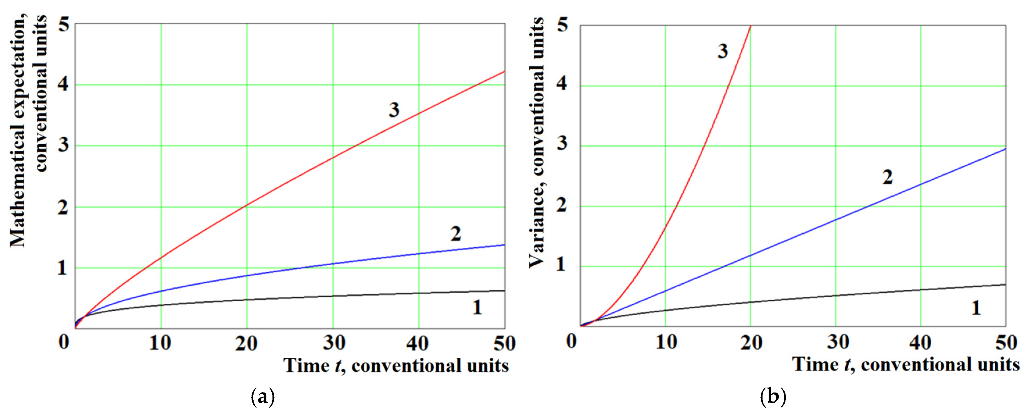
Let us analyze the behavior of the time dependences of the mathematical expectation ${\mu }_{\alpha ,\beta }\left(t\right)$ and dispersion ${\sigma }_{\alpha ,\beta }^2\left(t\right)$. For simulation modeling, we take the value $D=0.05$, $\alpha =1.70$ and consider two regions, $0<\beta /\alpha \le 0.50$ and $0.50<\beta /\alpha \le 0.865$. Figure 2a shows the results of the theoretical calculation of the mathematical expectation using Equation (8) ${\mu }_{\alpha ,\beta }(t)={\displaystyle \frac{D^{1/\alpha }·t^{\beta /\alpha }}{\Gamma \left[\frac{\beta }{\alpha }+1\right]}}$, and Figure 2b shows the dispersion (Equations (9) and ${\sigma }_{\alpha ,\beta }^2\left(t\right)={\displaystyle \frac{{2D}^{2/\alpha }·t^{2\beta /\alpha }}{\Gamma \left[2\frac{\beta }{\alpha }+1\right]}}$). Curves 1 in Figure 2 and Figure 3 are plotted for $\beta /\alpha =0.3$; curves 2 for $\beta /\alpha =0.5,$ and curves 3 for $\beta /\alpha =0.8$.

Figure 2 shows that in the region $0<\beta /\alpha \le 0.50$, the behavior of the graphs for the mathematical expectation and dispersion is very similar; they grow more monotonically than the linear dependence (see line 2 in Figure 2b), and at $0.50<\beta /\alpha$, a stronger growth is observed.

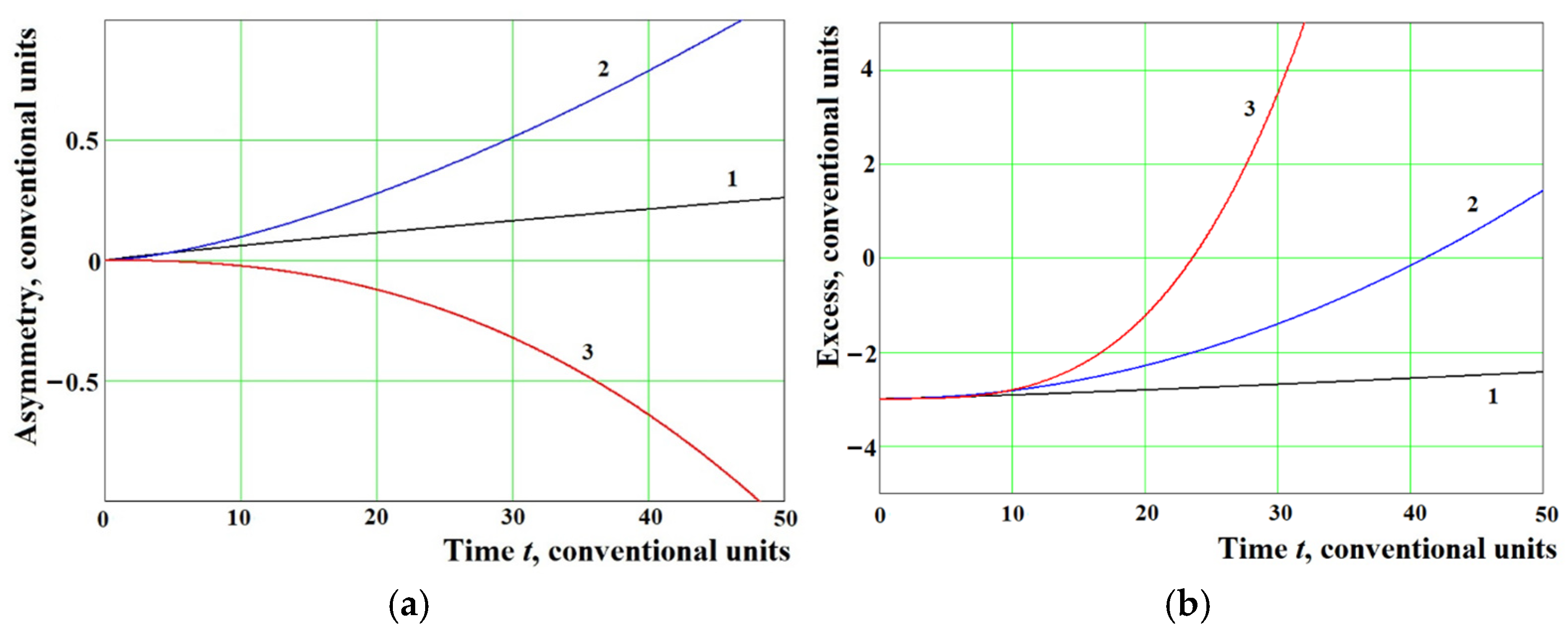
Figure 3 shows the results of the calculation ${As}_{\alpha ,\beta }\left(t\right)$ of asymmetry using Equation (10) (see Figure 3a) and ${Ex}_{\alpha ,\beta }\left(t\right)$ of excess using Equation (11) (see Figure 3b).

The dependence of the amplitude asymmetry on the time interval of its calculation in the region $0<\beta /\alpha \le 0.35$ is almost linear. In the region $0.35<\beta /\alpha \le 0.62,$ there is growth in the positive range of values. In the region $0.62<\beta /\alpha$, there is a decrease in growth, and the dependence goes into the region of negative values. The excess can be in the region of negative values at short times, and with an increase in the time interval of amplitude calculation, their excess goes into the positive region.

6. Analysis of the Dynamics of Time Series of Non-Local Processes in Complex Systems

To compare the results that can be obtained using the developed model and the results of observations of real processes, it is necessary to find time series whose characteristics would be non-local in time $t$ and state $x$.

To analyze the non-locality of the time series dynamics and determine their characteristics, the Hurst normalized range method [34] can be used, which allows determining their fractal dimension and classifying the type of behavior. It is possible to normalize the range of the values of the levels of the series R by the standard deviation of the values of the levels of the series S and present their ratio (normalized range) as an equation: $⁄S=C{n}^H$ (after logarithm $log[R⁄S]=H\times log\left[n\right]+log\left[C\right]$), where $C$ is a certain constant, n is the number of observations (levels of the series) that make up the time series ($TS$) under consideration, and the exponent $H$ is the so-called Hurst coefficient or exponent. The presence of breaks in the dependence of $ln \{R⁄S\}$ on $ln\left(n\right)$ may indicate the presence of characteristic time scales and/or periodicities. The value of the coefficient $H$ allows classification of time series by the nature of their behavior.

For a random process with independent increments and finite dispersion, it has been rigorously proven [35] that the $H$ exponent is equal to $0.5$.

The difference of the Hurst exponent from $0.5$ reflects the fractal properties of the processes generating time series. At $H>0.5$, the observed tendency of the process is maintained (the property of persistence), and at $H<0.5$, the tendency changes to the opposite (anti-persistence); i.e., the growth of the observed value is replaced by a decrease and vice versa [36].

As an example of time series reflecting complex processes with a strong influence of the human factor, we can consider, for example, the dynamics of changes in voter preferences during the US presidential elections. Figure 4 shows, as an example, time series of voter preferences in the Clinton–Trump presidential campaign of 2016 [37].

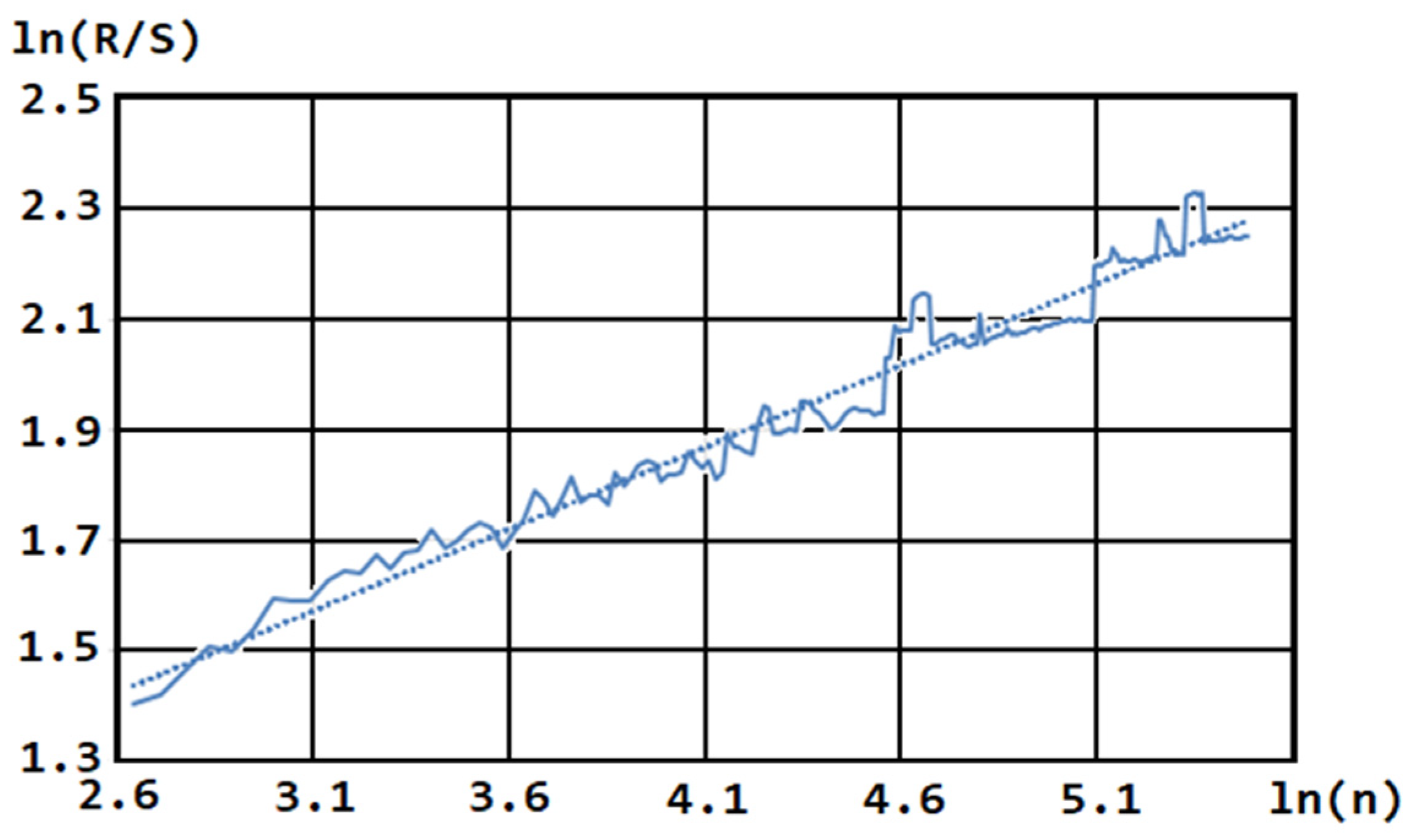
Figure 5 shows, as an example, a plot of the natural logarithm of $R/S$ versus the natural logarithm of the number of observations (series levels—$n$) for the preferences of voters voting for Trump in the 2016 US presidential campaign.

After processing the time series of US presidential election campaigns in 2016–2020 [37], we can obtain the following linear dependencies $ln\{R ⁄ S\}$ on $ln\left(n\right)$:

• In 2020: Biden—$y=0.46x-0.01$; Trump—$y=0.48x-0.05$;
• In 2016: Trump—$y=0.30x+0.66$; Clinton—$y=0.36x+0.48$;
• In 2012: Obama—$y=0.29x+0.66$; Romney—$y=0.22x+0.99$;
• In 2008: Obama—$y=0.30x+0.69$; McCain—$y=0.32x+0.60$.

To confirm the conclusion about the linear approximation, we can examine the behavior of the residuals and test the hypothesis that they are normally distributed with a mean value equal to zero and have a homogeneous dispersion. The calculated value of the mathematical expectation for the distribution of residuals is $0.25$, and the dispersion is $0.13$.

Testing the hypothesis about the slope (two-sample F-test for dispersions) shows that the dispersion of the residuals (calculated relative to the trend line) is significantly less than the dispersion of the deviation of the linear regression points from the mean value of the observed data. It is equal to $2.51$ ($0.13<<2.51$).

Thus, from the obtained data, we can conclude that the distribution of the residuals is very close to normal, and the obtained regression is significant.

Note that in all cases for the studied time series, the value of $H$ is significantly less than $0.5$, and, therefore, the observed time series is antipersistent (ergodic). Since the value of the Hurst coefficient is significantly different from $0.5$, it follows that the structure of these series has fractality [38], and the processes described by it can have short-term memory (aftereffect). Hurst also suggested that the shift in values from $0.5$ occurs due to the existence of memory.

It should be noted that the study of fractality of time series allows us to obtain forecasts of their dynamics, which are useful from a practical point of view. In [39], issues of fractality analysis of heart rate time series were considered.

The aim of the work was to determine the parameter of fractal dimension calculated for a sequence of RR interval durations, to identify the boundaries of its change for healthy and sick patients, as well as the possibility of using it as an additional factor in identifying cardiac pathology.

A significant difference of the Hurst exponent from a value equal to $0.5$ indicates that the observed characteristics of the time series under study may differ significantly from the normal distribution law.

To determine the properties of the observed time series and the distribution functions of their parameters (probability density), for example, the magnitude of the amplitude of the change in the levels of the series depending on the time interval of calculation of this amplitude (this is necessary for the analysis of the characteristics and dynamics of the observed processes), we can use the following algorithm developed by us:

• First, you can set the size of the “sliding window” (the time interval between the observed levels of the series, for example, one day, two days, three, etc.) and select data from the time series for the specified time range (the size of the “sliding window”).
• Next, based on the selected data, it is possible to calculate the amplitudes of the change in the series levels for various selected time intervals (sizes of the “sliding window”).
• Then, one can sort in ascending order (from negative to positive) the sets of values obtained for each of the measured intervals, and, for each size of the “sliding window”, construct histograms of the distribution density of the deviation amplitudes.
• Then, using the obtained histograms, it is possible to calculate the distribution moments (mean value: mathematical expectation, dispersion, asymmetry, excess) for the selected time intervals for calculating the deviation amplitudes.

Next, we can construct dependencies for the mathematical expectation, dispersion, asymmetry, and excess of the amplitudes of deviations of the series levels from the time intervals of calculation of these amplitudes (the sizes of the “sliding window”).

The study of the dependence of the mathematical expectation, dispersion, asymmetry (the third moment of distribution), and excess (the fourth moment of distribution) of the amplitudes of deviations of the levels of time series on the calculation time intervals (the sizes of the “sliding window”) allows us to determine whether the studied time series are non-stationary and to use the observed characteristics to build a model of their evolution, which is necessary for predicting their dynamics. The observed value of the mathematical expectation, dispersion, asymmetry, and excess were calculated using the following equations:

$$\mathsf{\mu }(t)={\displaystyle \frac{\sum _{j=1}^N{x}_j(t)}{{\sum }_{l=1}^M{n}_l}}$$

$${\sigma }^2(t)={\displaystyle \frac{\sum _{j=1}^N{\left\{x_j(t)\right\}}^2}{{\sum }_{l=1}^M{n}_l}}$$

$$As(t)={\displaystyle \frac{\sum _{j=1}^N{\left\{x_j\left(t\right)-\mathsf{\mu }(t)\right\}}^3}{{\sigma }^3{\sum }_{l=1}^M{n}_l}}$$

$$Ex\left(t\right)={\displaystyle \frac{\sum _{j=1}^N{\left\{x_j\left(t\right)-\mathsf{\mu }\left(t\right)\right\}}^4}{{\sigma }^4{\sum }_{l=1}^M{n}_l}}-3$$

and ${\sum }_{l=1}^M{n}_l$—is calculated based on the number of amplitude values $n_l$.

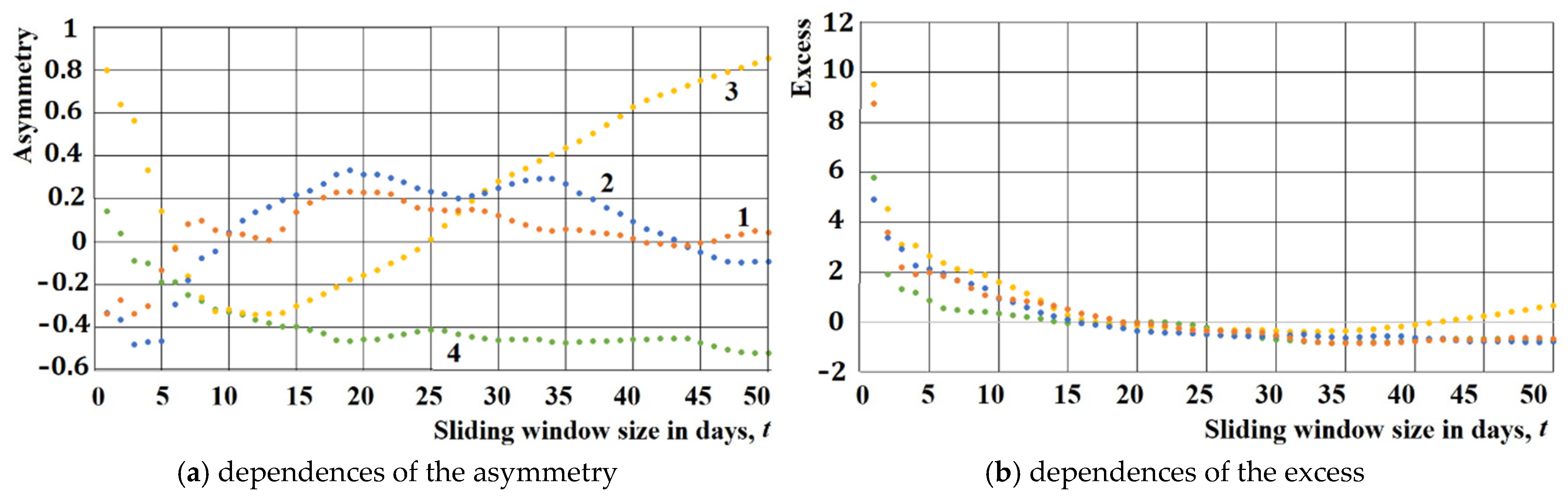
Figure 6 shows the dependences of the mathematical expectation (see Figure 6a) and dispersion (see Figure 6b) of the amplitudes of the time series levels on the time interval of their calculation for voter preferences in the US presidential election campaigns in 2008–2020 (for their winners); in Figure 7a—asymmetry, in Figure 7b—excess. Curves 1 in Figure 6 and Figure 7 are constructed after analyzing the change in Obama’s popularity in 2008; curves 2—Obama (2012), curves 3—Trump (2016) and curves 4—Biden (2020). The mathematical expectation, dispersion, asymmetry, and excess were calculated for the entire period of each of the election campaigns.

Figure 6 and Figure 7 show that the values of the mathematical expectation of the amplitudes, their dispersion, asymmetry, and excess depend in a complex nonlinear way on the time interval of calculation of these amplitudes (“sliding window”), which indicates that the studied time series are not stationary.

For example, when performing the Poisson distribution for a stationary time series $\rho \left(x,t\right)={\displaystyle \frac{1}{2\sqrt{\pi \mathrm{D}t}}}{·e}^{-{\displaystyle \frac{x^2}{4·D·t}}}$, the value of the mathematical expectation $\mu \left(t\right)$ should be equal to zero (or be a constant):

$$\mu (t)={\int }_{-\mathrm{\infty }}^{+\mathrm{\infty }}x·\rho \left(x,t\right)dx={\displaystyle \frac{1}{2\sqrt{\pi \mathrm{D}t}}}{\int }_{-\mathrm{\infty }}^{+\mathrm{\infty }}{x·e}^{-{\displaystyle \frac{x^2}{4·D·t}}}dx=0$$

where x is the amplitude value, and t is the time interval for its calculation (the value of the “sliding window”).

In addition, when the Poisson distribution is implemented, the amplitude dispersion should show a linear dependence on the size of the “sliding window”:

$${\sigma }^2\left(t\right)={\int }_{-\mathrm{\infty }}^{+\mathrm{\infty }}{x}^2\rho \left(x,t\right)dx={\displaystyle \frac{1}{2\sqrt{\pi \mathrm{a}t}}}{\int }_{-\mathrm{\infty }}^{+\mathrm{\infty }}{x}^2{e}^{-{\displaystyle \frac{x^2}{4·a·t}}}dx = 2 at$$

For the studied time series, a deviation of the distribution from the Poisson law is observed, which indicates that the observed time series are non-stationary.

The dependences of the values of the mathematical expectation and dispersion of the amplitudes of the change in the levels of time series on the time interval of calculating these amplitudes, presented in Figure 6, have a form close to the dependence $~\sqrt[\beta ]{t}$, where $\beta >0$ is some positive, possibly fractional number. This indicates that the process has fractality in time, and it can be assumed that when modeling the dynamics of non-stationary time series based on differential equations, they can contain a fractional derivative in time of any value.

The complex relationship between the asymmetry of the amplitude distribution and the time interval of their calculation (see Figure 7a) suggests that the process under investigation exhibits some degree of self-organization.

This is evidenced by the varying “drift” of the characteristics of the time series towards a certain state for different time intervals used in the asymmetry calculations. In the examined cases (see Figure 7b), it is observed that for small time intervals in amplitude calculations, the value of the distribution excess is significant.

Conversely, for larger “sliding windows”, this value gradually decreases to zero, approaching the excess characteristic of the Poisson distribution, which may further indicate the self-organization of the processes.

Processing and analysis of the observed data allows us to draw a number of conclusions:

• The time series describing the processes under consideration are non-stationary (the values of the mathematical expectation and dispersion of the amplitudes depend in a complex way on the time interval of calculation of these amplitudes (“sliding window”) $~\sqrt[\beta ]{t}$, where $\beta >0$ is some positive, possibly fractional number), which indicates that the observed processes have fractality in time, and fractional differential equations can be used in their modeling.
• Analysis of the observed non-stationary time series shows that the processes they describe have fractality and short-term memory (the value of the Hurst exponent is significantly less than $0.5$).
• The complex dependence of the asymmetry and excess of the amplitudes of the change in the levels of the series on the time interval of its calculation indicates that for the process under consideration, some self-organization is observed, which is manifested in the fact that for different time intervals there will be different asymmetries, and the value of the excess at large intervals tends to that characteristic of the Poisson distribution.
• Comparison of Figure 2 (theoretical calculation) and Figure 6 (results of processing the observed data) shows that the observed dependencies of the mathematical expectation and dispersion are in good agreement with those calculated theoretically, using the developed model, if the value of $\beta /\alpha$ lies in the region $0<\beta /\alpha \le 0.50$.
• The observed dependencies of the asymmetry and excess of the amplitudes of deviations of time series on the time interval of calculation of these amplitudes are complex in nature and comparison of their behavior with theoretical calculations is very difficult and does not allow for unambiguous conclusions.

The model of approximating functions of the distribution density of parameters of non-stationary time series should consider all the above characteristics of the observed processes, and considering the fact that the processes under consideration are non-local in time t and state x, then for their modeling, one can try to use fractional differential equations with an arbitrary value of the orders of derivatives.

7. Evaluation of the Accuracy of the Model in Forecasting the Dynamics of Time Series

Let us consider the possibility of using the proposed model to forecast the dynamics of time series, for example, the electoral campaigns of the US presidential elections in 2008–2020. For validation and accuracy assessment, we will use data from the resource [2].

The choice of the optimal sample size of the time series for finding the model parameters $D$, $\alpha$, and $\beta$ is determined by the following factors. If it is taken very large, then it will include a significant number of information events that can cause high volatility. If it is taken too short, then the reduction in the amount of statistical data will introduce a significant error, which will negatively affect the accuracy of determining the model parameters.

Let us define the parameters of the model and evaluate its accuracy using the following algorithm:

• Let us take the original time series and consider some part of it included in the selected time interval ($\mathsf{\Delta }{t}_n$), which will contain n-values of the series levels.
• Next, for the selected part of the time series, we find the differences between its different $n$ levels (deviation amplitudes). We denote these differences as ${\mathsf{\Delta }}_j$, where $j$ is the number of intervals between the selected levels. For example, if the number of values of the series levels $n=15$ was selected, then the number of values of the amplitudes ${\mathsf{\Delta }}_1$ will be equal to 14 (the nearest levels); the amplitudes ${\mathsf{\Delta }}_2$ separated by $j=2$, two intervals between the nearest levels, will also be equal to 14; the amplitudes ${\mathsf{\Delta }}_3$ separated by $j=3,$ three intervals between the nearest levels, will be equal to 13 (levels separated by three intervals); the amplitudes ${\mathsf{\Delta }}_4$ separated by $j=4$, four intervals between the nearest levels, will be equal to 12, etc. The last value of the number ${\mathsf{\Delta }}_j$ will be determined by the fact that it must be statistically significant for subsequent averaging; for example, there must be at least four values.
• Then we find the square of the value of each difference ${\mathsf{\Delta }}_j$ and average them over the total amount (we find the observed value ${\sigma }_{\alpha ,\beta }^2\left(t\right)$). Next, using Equation (8) for ${\sigma }_{\alpha ,\beta }^2\left(t\right)$, we find the parameters of the model. ${\sigma }_{\alpha ,\beta }^2\left(t\right)$ gives the advantage, compared to using the mathematical expectation, ${\mu }_{\alpha ,\beta }\left(t\right)$ that we can ignore the sign of the change ${\mathsf{\Delta }}_j$. Taking the logarithm ${\sigma }_{\alpha ,\beta }^2\left(t\right)$ (see expression 9), we obtain

  $$ln\left\{{\sigma }_{\alpha ,\beta }^2\left(j\right)\right\}=ln\left\{{\displaystyle \frac{2D^{2/\alpha }}{\mathrm{\Gamma }\left[2\frac{\beta }{\alpha }+1\right]}}\right\}+2{\displaystyle \frac{\beta }{\alpha }}ln(j)$$
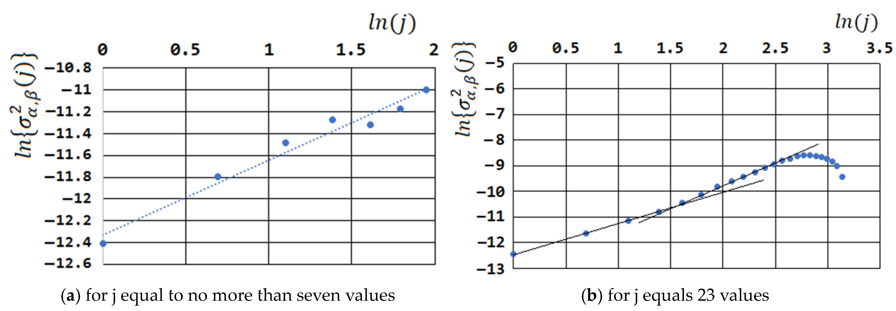
  Having processed the observed data (see Figure 7) using the obtained linear dependence, we determine the tangent of its slope ($tg\phi =0.69$), and we can calculate the value of $\beta /\alpha =0.35$ and $\mathrm{\Gamma }\left[2{\displaystyle \frac{\beta }{\alpha }}+1\right]$. Further, by extrapolating the obtained linear dependence to the axis, $ln\left\{{\sigma }_{\alpha ,\beta }^2\left(j\right)\right\}$ we can find $D^{2/\alpha }$. Figure 8 shows the linearization of the observed data for a randomly selected part of the time series with a length of 25 days, showing the change in the preferences of Trump voters in 2016 (Figure 8a for j equal to no more than seven values, Figure 8b for j—23 values).
• Then, we can calculate the predicted amplitude values ${∆}_j^P$ for each of the time intervals $j=1, 2, 3\dots$. For this, we can use the found values of the model parameters and the equation for the mathematical expectation:
• ${∆}_j^P=\mu \left(j\right)={\displaystyle \frac{D^{1/\alpha }·t^{\beta /\alpha }}{\Gamma \left[\frac{\beta }{\alpha }+1\right]}}$. Next, using the last observed value of the time series level in the time interval $∆$t_n and the predicted change ${∆}_j^P,$ we can build a forecast for its selected depth j (j determines the forecast time interval ${∆t}_j$). Note that when finding the forecast value, it is necessary to consider the trend observed in the interval ${∆t}_n$. If a general decrease is observed, then ${∆}_j^P$ is subtracted from the last observed value; if an increase, then it is added.
• Next, using the predicted value of the series level and the observed value, we can determine the relative forecast error by modulus. To achieve this, we subtract the observed value from the predicted value and divide by the value of the observed value.
• We return to the original time series and shift ${∆t}_n$ by one level count number of the series to the right. The new interval will also contain n levels, but there will be only one new one in it—the one on the far right.
• Next, we perform steps 1–6 of this algorithm until all values of the levels of the original time series have been processed.
• Then, for a given selected ${\tau }_n$ and each $j$ selected in it, we determine the average error over all predictions made.
• Next, we return to point 1 of this algorithm and increase the time interval for finding the parameter ${∆t}_n$_, i.e., the number of ${\tau }_n$-values of the series levels included in it (for example, so that τ_n increases by 1). After that, we perform steps 1–8 of this algorithm until all the values of the levels of the original time series are processed.

Figure 9 shows 3D graphs of the dependence of the relative forecast error on the sample size ${\tau }_n$ and the forecast depth $t$, obtained based on the processing of observed data on voter preferences of the winners of the US presidential election campaigns in 2008–2020, using the previously described algorithm for determining the model parameters and assessing its accuracy. Figure 9a—Biden (2020), Figure 9b—Trump (2016), Figure 9c—Obama (2012), Figure 9d—Obama (2008).

When determining the accuracy of forecasting, the sample size range for determining the model parameters was considered from 10 to 100 days and the forecast depth from 1 to 100 days.

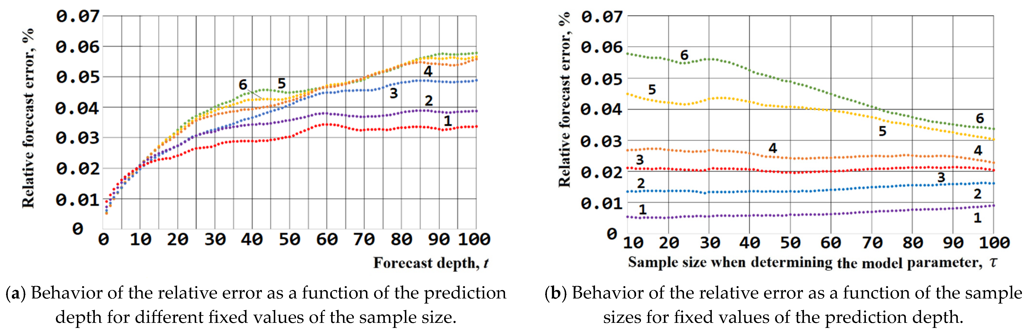
Figure 10 shows, as an example, cross-sections of the surface describing the dependence of the relative forecast error on the sample size τ_n and the forecast depth t for the preferences of Biden voters in 2020. Figure 10a illustrates the behavior of the relative error as a function of the prediction depth for different fixed values of the sample size (curve 1 for the sample size ${\tau }_n=100$, curve 2—${\tau }_n=75$, curve 3—${\tau }_n=50$, curve 4—${\tau }_n=20$, curve 5—${\tau }_n=15,$ and curve 6—${\tau }_n=10$), and Figure 10b as a function of the sample sizes for fixed values of the prediction depth (curve 1 for the prediction depth of 1, curve 2—5, curve 3—10, curve 4—15, curve 5—50, and curve 6—100). Curves 1–6 shown in Figure 10 are the result of processing the observed data using different sizes of time series samples.

The dependence of forecast accuracy on sample size ${\tau }_n$ and depth $t$ has a complex form with local maxima and minima, but their numerical characteristics allow us to draw the following conclusions:

• For any sample size ${\tau }_n$ used to determine the model parameters, in general, the accuracy of the forecast decreases with increasing depth (the relative error increases), which demonstrates the adequacy of the accuracy assessment methodology used.
• At a shallow depth of 1–2 days, the relative error is from 0.5–1.0% (for different winners) with a small sample of the series for determining the model parameters (10 days) and about 1.0–1.5% (for different winners) with a sample of 100 days.
• With a forecast depth of about 10–14 days, its relative error is practically independent of the sample size taken to determine the model parameters and is about 2.0–2.5% (Biden 2020), 3.0–3.5% (Trump 2016), and 1.5–2.0% (Obama 2012) for any sample. From a practical point of view, forecasts for 1–2 weeks are of the greatest interest for managing an election campaign, and given that acceptable accuracy in the proposed methodology can be ensured using small samples of the time series, the proposed forecasting method is technologically easy to implement.
• With a large forecast depth (about 100 days), the relative error is about 2.0 to 3.5% (for different winners) with a small sample of the series for determining the model parameters (10 days) and 3.4–6.9% (for different winners) with a sample of 100 days. The increase in forecast error with an increase in forecast depth also confirms the adequacy of the proposed accuracy assessment method.

Similar results are obtained when analyzing the preferences of voters of the losing candidates. In conclusion, it should be noted that all the results obtained show that the developed model of time series analysis shows a very high accuracy of forecasting the dynamics of electoral processes and can be used in practice.

8. Conclusions and Findings

As a result of the research, a new solution was obtained for the problem of finding the probability density function of the observation of the state $x$ of a certain process (for example, the magnitude of the deviation of the levels of a time series) from time $t$ (for example, the time interval for calculating the amplitudes of the deviation of the levels of a time series) for an infinite axis based on a fractional differential equation of the diffusion type. The presented solution differs from the existing ones in that it was obtained for arbitrary values of the orders of derivatives. The solutions described in the literature, as a rule, are considered in the case when the value of the fractional derivative with respect to time $\beta$ lies in the range $0<\beta <1$, and the fractional derivative with respect to state $\alpha$ (the variable describing the state of the process) is in the range $1<\alpha <2$. The presented solution allows us to consider any ranges for $\alpha$ and, if the inequality $0<\beta /\alpha \le 0.865$ is satisfied, for their ratio $\beta /\alpha$. When solving practical problems of analyzing and forecasting the dynamics of time series of complex processes, it may turn out that the condition $0<\beta \le 1$ and $1\le \alpha \le 2$ is a limitation of the model, and the values of $\alpha$ and $\beta$ may go beyond the specified ranges.

In practical terms, for example, when analyzing the dynamics of time series, it is necessary to determine the parameters of the model using the observed sample of the series. Once determined, they can be used to predict new values of series levels at a given point in time.

Such tasks are widespread, not only in sociology, but also in economics, for example, when predicting financial processes (changing stock indicators, etc.). In order to ensure the necessary prediction accuracy, it is necessary to make as accurate a determination of model parameters as possible.

The research conducted by us showed that the received estimates of high precision of forecasting very often are reached only if α and β lie out of ranges 0 < β ≤ 1 and 1 ≤ α ≤ 2.

In this regard, existing solutions cannot be used, because they limit the analysis only to the specified ranges, and the accuracy of forecasts is significantly reduced.

In addition, the existing solutions of fractional diffusion equations do not always allow obtaining various moments of the partition function, for example, the mathematical expectation of deviations of the time level.

In particular, [7,26] indicates that all moments of the solutions described in the literature exist only at α = 2, while the solution presented by us shows that it is possible to find moments of any order, which also expands the possibilities of its application for practical purposes compared to existing ones.

In the analysis of observed data, for example, it is possible to define dependence of expected value of amplitude of a deviation between row levels from an interval of calculation of amplitude. However, the existing models with ranges of values of fractional derivatives 0 < β ≤ 1 and 1 ≤ α ≤ 2 indicate that mathematical expectation does not exist, and this does not allow them to be applied to the processing of observed data, while our proposed solution removes this contradiction.

Analysis of the developed model shows that when changing the values of $\alpha$ and $\beta$, a change in the scales of the presentation of the results of simulation modeling is observed, but the general form of the dependencies is preserved for all the studied areas, which is clearly seen in a pairwise comparison of Figure 1a,d, Figure 1b,e, and Figure 1c,f.

As the time t increases, the height of the distribution function graphs decreases and the width increases, and they remain symmetrical relative to the line passing vertically through zero. However, in the region $0.50<\beta /\alpha \le 0.865$, although the graph is symmetrical, the position of the maxima shifts to the right and to the left with increasing t (see Figure 1a,d).

It should also be noted that as x increases, the probability density function ${\rho }_{\alpha ,\beta }(x,t)$ quickly drops to zero.

When the value of the coefficient $D$ changes, a change in the scales of the presentation of the results of simulation modeling is observed, but the general form of the dependencies for the two selected areas is preserved.

The indices of fractional derivatives may take integer values; however, when their ratio aligns with the characteristics of the analyzed domains, the behavior of the probability density function ${\rho }_{\alpha ,\beta }(x,t)$ corresponds to the patterns illustrated in Figure 1a–f.

Figure 2 shows that in the region $0<\beta /\alpha \le 0.50$, the behavior of the graphs for the mathematical expectation and dispersion is very similar; they grow more monotonically than the linear dependence (see line 2 in Figure 2b).

The analysis of the obtained model shows that it is not inconsistent, and the behavior of the moments of the distribution function (mathematical expectation and dispersion) obtained theoretically coincides with those observed in practice for the time series of electoral processes of the US presidential elections in 2008, 2012, and 2016 (see comparison of Figure 2 and Figure 6). The observed dependencies are in good agreement with those calculated theoretically using the developed model if the value of $\beta /\alpha$ lies in the region $0<\beta /\alpha \le 0.50$.

The proposed model for describing the dynamics of time series allows us to develop a forecasting algorithm with high accuracy. At a shallow forecast depth of 1–2 days, the relative error is from 0.5–1.0% (for different winners) with a small sample of the series for determining the model parameters (10 days) and about 1.0–1.5% (for different winners) with a sample of 100 days. With a forecast depth of about 10–14 days, its relative error is practically independent of the sample size taken to determine the model parameters and is about 2.0–2.5% for any sample. With a large forecast depth (about 100 days), the relative error is about 2.0 to 3.5% (for different winners) with a small sample of the series for determining the model parameters (10 days) and 3.4–6.9% (for different winners) with a sample of 100 days.

Similar results are obtained when analyzing the preferences of voters for the losing candidates.

For any sample size τ_n employed in determining the model parameters, the forecasting accuracy generally decreases with increasing depth, as evidenced by the growth in relative error. This trend underscores the validity of the applied accuracy assessment methodology.

From a practical point of view, forecasts for 1–2 weeks are of the greatest interest for managing an election campaign, and given that acceptable accuracy in the proposed methodology can be ensured using small samples of the time series, the proposed forecasting method is technologically easy to implement.

Summing up our research, we can say the following:

• The solution we obtained for the fractional diffusion differential equation of the boundary value problem ${\left.\rho (x,t)\right|}_{\mathrm{x}\to -\mathrm{\infty }}={\left.\rho (x,t)\right|}_{\mathrm{x}\to \mathrm{\infty }}=0$ with the initial condition $\rho \left(x,0\right)=\delta \left(x-0\right)$, the distribution function $\rho (x,t)$ o meets the normalization condition and passes in the limit case at α = 2 and β = 1 into a Poisson distribution (i.e., in a broad sense, it can be a distribution function).
• Unlike existing solutions of the fractional diffusion equation, the model presented in this article allows you to find any moments of the distribution function, while existing approaches allow you to find all moments only if α = 2. The solution described in this article allows us to remove the contradiction between the fact that, in practice, it is possible, for example, to calculate the mathematical expectation of deviations between the levels of the time series, and the existing models are not applicable because they claim that the mathematical expectation does not exist; i.e., they are not applicable for a possible description of the observed data.

The further direction of our research will focus, firstly, on a strict proof in the form of theorems of the results we obtained. Secondly, we plan to continue our research described in the work [40]. In this article, we examined the schemes of probabilistic transitions between process states that can be observed in complex systems and obtained a fractional-differential telegraph-type equation with multiple (in time: β, 2β, 3, . . . and the state: α, 2α, 3α, . . .) orders of derivatives.

If we consider the derivative of the form ${\displaystyle \frac{{\partial }^{\beta }\mathrm{\rho }(x,t)}{\partial t^{\beta }}}$ as the rate of change of process states over time, then the term of the form ${\displaystyle \frac{{\partial }^{2\beta }\mathrm{\rho }\left(x,t\right)}{\partial t^{2\beta }}}$ can be considered as the acceleration of the process. Of interest is the solution of the resulting telegraph equation for the boundary value problem ${\left.\rho (x,t)\right|}_{\mathrm{x}\to -\mathrm{\infty }}={\left.\rho (x,t)\right|}_{\mathrm{x}\to \mathrm{\infty }}=0$ with the initial condition $\rho \left(x,0\right)=\delta \left(x-0\right)$ and comparing it with the resulting solution for the fractional diffusion equation. It is possible that this will provide new opportunities for analyzing and describing the dynamics of time series in order to predict the evolution of the processes they describe.