Statistical Inference on the Shape Parameter of Inverse Generalized Weibull Distribution

Abstract

In this paper, we propose statistical inference methodologies for estimating the shape parameter $\alpha$ of inverse generalized Weibull (IGW) distribution. Specifically, we develop two approaches: (1) a bounded-risk point estimation strategy for $\alpha$ and (2) a fixed-accuracy confidence interval estimation method for $\alpha$. For (1), we introduce a purely sequential estimation strategy, which is theoretically shown to possess desirable first-order efficiency properties. For (2), we present a method that allows for the precise determination of sample size without requiring prior knowledge of the other two parameters of the IGW distribution. To validate the proposed methods, we conduct extensive simulation studies that demonstrate their effectiveness and consistency with the theoretical results. Additionally, real-world data applications are provided to further illustrate the practical applicability of the proposed procedures.

1. Introduction

Weibull distribution, which is named after the Swedish mathematician Waloddi Weibull [1], has been widely used in diverse disciplines to study many different issues. Some examples are food science, survival analysis, reliability engineering, and weather forecasting. One is referred to Lai et al. (2006) [2] for some detailed discussions on the applications of this model. Moreover, Weibull distribution is related to many other probability distributions, such as the exponential distribution and the Rayleigh distribution, which makes it a more versatile and flexible model.

The probability density of a random variable, S, following Weibull distribution is

$$f(s;\lambda ,k)={\displaystyle \frac{k}{\lambda }}{\left({\displaystyle \frac{s}{\lambda }}\right)}^{k-1}{e}^{-{\left({\displaystyle \frac{s}{\lambda }}\right)}^k},s\ge 0,$$

(1)

with $k>0$ being the shape parameter and $\lambda >0$ being the scale parameter.

Weibull distribution accommodates increasing and decreasing failure rates. However, it does not allow non-monotone failure rates, while the non-monotone failure rate situation is very common in real life. Particularly, engineering and biological sciences often involve bathtub-shaped failure rates. Thus, a generalized Weibull distribution handling bathtub failure rate was introduced by [3], and then it was further explored and applied in [4]. They named it exponentiated Weibull distribution (EW). The added shaped parameter allows the distribution to represent increasing, decreasing, and bathtub-shaped hazard functions. Then, Mudholkar and Hutson (1996) [5] introduced a generalized form of Weibull distribution, which goes beyond the EW distribution. This generalization provides even greater flexibility than the EW distribution, with applications specifically highlighted in survival data and more complex time-to-event analyses.

Over the last few years, many variations of Weibull distribution have been introduced. Lai (2014) [6] presented a thorough discussion of generalized Weibull distributions. One can find the details, such as the density function, moment function, and hazard rate function, for many different variations of Weibull distribution, such as inverse Weibull distribution, exponentiated Weibull distribution, and Stacy’s Weibull distribution. Shama et al. (2023) [7] proposed a modified generalized Weibull distribution, providing theoretical insights and demonstrating applications across various fields. Through applications, the authors demonstrated the modified distribution’s effectiveness in fitting real-world data across fields such as reliability engineering, survival analysis, and environmental studies. Alsaggaf et al. (2024) [8] introduced a new generalization of the inverse generalized Weibull distribution, enhancing estimation methods and exploring its applications in medicine and engineering. There are other generalized distributions and their inversed versions. XLindley is a great example to mention here. Gemeay et al. (2023) [9] developed a modified XLindley distribution, detailing its properties, estimation techniques, and applications in reliability and risk assessment. Beghriche et al. (2023) [10] introduced inverse XLindley distribution, examining its properties and demonstrating its applications in modeling lifetime data.

Statistical inference is frequently performed using an existing data set or a data set that is readily accessible. However, some statistical inference problems have no fixed-sample-size solutions, according to [11]. And that is why sequential analysis is necessary and important, as it provides a way to decide on the necessary sample size and conducts statistical inference under certain accuracy requirements in the meantime. Anscombe (1952), Chow and Robbins (1965) [12,13] provided sequential procedures, creating a fixed-width confidence interval for the mean parameter of a normal distribution when the variance is also unknown. Sequential procedures for point estimation when one wants to limit the risk to its minimum or a certain value are also well developed in the literature; one may refer to Mukhopadhyay (1987), Zacks and Mukhopadhyay (2006), and Mahmoudi et al. (2019) [14,15,16]. A comprehensive review of sequential methodologies can be found in [17]. Recently, Mukhopadhyay and Banerjee (2014) [18] developed a new class of fixed-accuracy confidence interval methodologies with a confidence coefficient for the mean of a negative binomial distribution. They provided appropriate ways to develop confidence intervals that lie completely inside the parameter space when an unknown parameter under consideration is positive. In light of this wonderful idea, many other confidence interval estimation methodologies were developed. Mukhopadhyay and Zhuang (2016) [19] created a fixed-accuracy confidence interval for the parameter from Fisher’s “Nile” example; Bapat (2018) [20] discussed fixed-accuracy confidence intervals for $P(X<Y)$ under bivariate exponential models, and Zhuang et al. (2020) [21] developed a fixed-accuracy confidence interval of $P(X>c)$ for a two-parameter gamma population.

In this paper, we will focus on the statistical inference of the $\alpha$ parameter of the inverse generalized Weibull distribution, including both point estimation and confidence interval estimation procedures. If a random variable, X, follows inverse generalized Weibull distribution (IGW), then its probability distribution function (p.d.f.) can be written as follows:

$$f(x,\alpha ,\beta ,\lambda )=\alpha \beta {\lambda }^{\beta }{x}^{-(\beta +1)}{e}^{-{\left({\displaystyle \frac{\lambda }{x}}\right)}^{\beta }}{\left(1-e^{-{\left({\displaystyle \frac{\lambda }{x}}\right)}^{\beta }}\right)}^{\alpha -1},x\ge 0.$$

(2)

with $\alpha ,\beta ,\lambda >0$. Here, $\alpha$ is the shape parameter that we will be focusing on, and we will discuss it in cases where $\beta$ and $\lambda$ are unknown and known to us. To maintain brevity and consistency, we will refer to the shape parameter as $\alpha$ throughout this paper.

It is in the light of [22] that we used the IGW simplified name for the distribution. This distribution is also highly related to the EW distribution we mentioned earlier in [3,4]. However, the EW distribution is exponentiated Weibull, while the distribution we investigate here is exponentiated inverse Weibull. $\alpha$ is an the exponentiation parameter. It is an important parameter that controls how the distribution behaves, particularly in terms of the tail heaviness and shape. To the best of our knowledge, we did not find any literature on bounded-risk point estimation or confidence interval estimation of $\alpha$, especially when one wants to use a minimal required sample with the required accuracy.

The estimation of parameters from exponentiated distributions is not rare in the literature. Mudholkar and Srivastava (1993) [3] discussed the exponentiated Weibull distribution and used maximum likelihood estimation (MLE) to estimate the parameters. NAG routines (COSNCF and COSPBF) were used to solve the MLE. Balakrishnan and Sandhu (1995) [23] used MLE and the method of moments for estimating the parameters of the exponentiated exponential distribution. They also emphasized the flexibility introduced via the exponentiation parameter $\alpha$, which allows for a wider variety of decay rates in modeling lifetime or reliability data. Sharma and Shanker (2010) [24] introduced the exponentiated generalized exponential distribution, which generalizes both the exponential and Weibull distributions by incorporating an exponentiation parameter $\alpha$. They also discussed using MLE to estimate all parameters of the EGE distribution, including $\alpha$, but the likelihood function is nonlinear and requires numerical methods. Similarly, Zhao and Zhang (2012) [25] explored exponentiated Pareto distribution and investigated the MLE method for estimating all parameters through numerical optimization techniques. In this work, we provide methodologies for estimating $\alpha$ through a well-designed procedure for both point estimation and confidence interval estimation. Our methods require the least amount of sample observations while satisfying the required accuracy in estimation risk or confidence level.

We want to emphasize that it is common in the literature that one may focus on estimating one parameter or even the function of one parameter while assuming the other involved parameters are known. Zhuang et al. (2020) [21] developed fixed-accuracy confidence interval estimation methodologies for a function of the rate parameter when the shape parameter is both unknown and known. Chaturvedi and Pathak (2015) [26] developed Bayes estimation strategies for the reliability function under type II censoring for a three-parameter exponentiated Weibull distribution, assuming that one of the shape parameters is unknown while the other two parameters are known. Chaturvedi et al. (2022) [27] worked on sequential estimation for an inverse Gaussian mean when the coefficient of variation is known.

The structure of the rest of the paper is as follows: In Section 2, we start with the maximum likelihood estimator of the shape parameter of the inverse generalized Weibull distribution. We propose the bounded-risk point estimation for the shape parameter, given that the other two parameters are known, in Section 2.1. We then introduce the fixed-accuracy confidence interval estimation for the shape parameter, regardless of the other two parameters, in Section 2.2. Section 2 also includes appealing properties for both inference methodologies. Section 3 discusses simulation studies to double-validate the theoretical results, as well as real data analysis for illustrative purposes. We conclude in Section 5, sharing some final thoughts.

2. Idea Formulation

Let $x_1,\dots ,x_n$ be a random sample of size n from the IGW distribution following the p.d.f., as in (2); then, the likelihood function of the sample data is given by

$$L(X,\alpha ,\beta ,\lambda )=\prod _{i=1}^{n}f(x_i,\alpha ,\beta ,\lambda )=\prod _{i=1}^n\alpha \beta {\lambda }^{\beta }{x}_i^{-(\beta +1)}{e}^{-{\left({\displaystyle \frac{\lambda }{x_i}}\right)}^{\beta }}{\left(1-e^{-{\left({\displaystyle \frac{\lambda }{x_i}}\right)}^{\beta }}\right)}^{\alpha -1},$$

(3)

and then the log-likelihood function can be written as

$$\begin{array}{cc}\hfill & l(X,\alpha ,\beta ,\lambda )\hfill \end{array}$$

(4)

$$\begin{array}{cc}& =nlog\alpha +nlog\beta +n\beta log\lambda -(\beta +1)\sum _{i=1}^{n}log\left(x_i\right)-\sum _{i=1}^n{\left({\displaystyle \frac{\lambda }{x_i}}\right)}^{\beta }\hfill \end{array}$$

(5)

$$\begin{array}{cc}& +(\alpha -1)\sum _{i=1}^{n}log\left(1-e^{-{\left({\displaystyle \frac{\lambda }{x_i}}\right)}^{\beta }}\right).\hfill \end{array}$$

(6)

Thus, the maximum likelihood estimator (MLE) for the shape parameter $\alpha$ would be as follows:

$$\widehat{\alpha }=-{\displaystyle \frac{n}{{\sum }_{i=1}^{n}log\left(1-e^{-{\left(\frac{\lambda }{x_i}\right)}^{\beta }}\right)}}$$

(7)

2.1. Bounded-Risk Point Estimation

Start with n independent random observations of $X\sim IGW(\alpha ,\beta ,\lambda )$; if we decide to use the MLE for $\alpha$, $\widehat{\alpha }$, then the squared-error loss function would be

$$Loss(\widehat{\alpha },\alpha ;X)={(\widehat{\alpha }-\alpha )}^2,$$

(8)

with $\widehat{\alpha }$ coming from (7), and $\alpha$ is the shape parameter of the distribution $IGW(\alpha ,\beta ,\lambda )$.

The risk associated with the squared-error loss would be

$$Risk(\widehat{\alpha },\alpha ;X)=E\left[{(\widehat{\alpha }-\alpha )}^2\right].$$

(9)

Before we get to the explicit form of the risk function, we would first address the distribution function of $\widehat{\alpha }$.

If we denote $Y=-{\sum }_{i=1}^{n}log\left(1-e^{-{\left({\displaystyle \frac{\lambda }{x_i}}\right)}^{\beta }}\right)$, then the MLE for $\alpha$ can be denoted as ${\displaystyle \frac{n}{Y}}$. One can easily check that $Y\sim Gamma(n,{\displaystyle \frac{1}{\alpha }})$. Thus, the distribution for $1/Y$ would be an inverse gamma distribution, denoted as $IG(n,\alpha )$. Using the properties of the inverse gamma distribution, when $n>2$

$$\begin{array}{cc}\hfill E[1/Y]=& {\displaystyle \frac{\alpha }{n-1}}\hfill \\ \hfill E[1/Y^2]=& {\displaystyle \frac{{\alpha }^2}{(n-1)(n-2)}}\hfill \end{array}$$

(10)

Then, one may derive the exact distribution for $\widehat{\alpha }\equiv Z$ with its pdf as the following.

$$f\left(z\right)={\displaystyle \frac{z^{-n-1}{n}^n{e}^{-n/\left(\alpha z\right)}}{\Gamma \left(n\right){\alpha }^n}},z>0$$

(11)

The following moments about $\widehat{\alpha }\equiv Z$ is derived when $n>2$

$$\begin{array}{cc}\hfill E\left[\widehat{\alpha }\right]=& \alpha {\displaystyle \frac{n}{n-1}}\hfill \\ \hfill E\left[{\widehat{\alpha }}^2\right]=& {\alpha }^2{\displaystyle \frac{n^2}{(n-1)(n-2)}}\hfill \end{array}$$

(12)

Now, it is time to come back to the risk function and derive its explicit form:

$$\begin{array}{cc}\hfill R_n\equiv Risk(\widehat{\alpha },\alpha ;X)=& E\left[{(\widehat{\alpha }-\alpha )}^2\right]\hfill \\ \hfill =& {\alpha }^2{\displaystyle \frac{n+2}{(n-1)(n-2)}}.\hfill \end{array}$$

(13)

We further require the estimation to have a fixed preassigned risk bound, say $\delta (>0)$, which means,

$$R_n={\alpha }^2{\displaystyle \frac{n+2}{(n-1)(n-2)}}<\delta .$$

(14)

Thus, upon solving the above equation in terms of n, we would require

$$n\ge {\delta }^{-{\displaystyle \frac{1}{2}}}\sqrt{0.25{\delta }^{-1}{\alpha }^4+3.5\alpha +0.25\delta }+0.5{\delta }^{-1}{\alpha }^2+1\equiv n^{\ast },\mathit{say}$$

(15)

Since $\alpha$ is unknown, there does not exist a fixed-sample solution to determine the size of the sample, $n^{\ast }$. Thus, we would turn to a sequential procedure,

$$N\equiv N\left(\delta \right)=\{n>2:n\ge {\delta }^{-{\displaystyle \frac{1}{2}}}\sqrt{0.25{\delta }^{-1}{\widehat{\alpha }}^4+3.5\widehat{\alpha }+0.25\delta }+0.5{\delta }^{-1}{\widehat{\alpha }}^2+1\},$$

(16)

with $\widehat{\alpha }$ being the MLE of the shape parameter $\alpha$ and $\delta$ being the fixed preassigned risk bound. The procedure is implemented in the following sense: One would start with a small number of sample observations; for example, let $n=10$ and check whether the condition in (16) is satisfied. If it is satisfied, one would use the 10 observations to conduct the point estimation for $\alpha$. If it were not satisfied, one would add one observation at a time until the condition would be satisfied. It is worth mentioning that $n>2$ is a basic requirement due to the aforementioned derivations, such as Equation (13).

Upon termination, we would have the following estimations for $\alpha$ and risk, R.

$$\begin{array}{cc}\hfill {\widehat{\alpha }}_N& =-{\displaystyle \frac{N}{{\sum }_{i=1}^{N}log\left(1-e^{-{\left(\frac{\lambda }{x_i}\right)}^{\beta }}\right)}},\hfill \end{array}$$

(17)

$$\begin{array}{cc}\hfill {\widehat{R}}_N& =E\left[{({\widehat{\alpha }}_N-\alpha )}^2\right].\hfill \end{array}$$

(18)

In the following, we establish interesting first-order properties of our proposed purely sequential procedure and the associated sample size N given in (16). We also include the properties of the estimation risk in Theorem 2.

Theorem 1.

For the purely sequential methodology (16), as fixed values of $\alpha ,\beta ,\lambda$ we have as $\delta \to 0$ the following:

(i)	$N/n^{\ast }\stackrel{P}{\to }1$
(ii)	$E\left[n^{\ast }/N\right]\to 1$
(iii)	$E\left[N/n^{\ast }\right]\to 1$

Proof. 

Part (i): Let ${\delta }^{-{\displaystyle \frac{1}{2}}}\sqrt{0.25{\delta }^{-1}{\widehat{\alpha }}_N^4+3.5{\widehat{\alpha }}_N+0.25\delta }+0.5{\delta }^{-1}{\widehat{\alpha }}_N^2+1$ be denoted as ${\widehat{\kappa }}_N$. From (16), one can thus obtain the following inequality:

$${\widehat{\kappa }}_N\le N\le {\widehat{\kappa }}_{N-1}+(m-1)I(N=m)+1,$$

where m denotes the fixed pilot sample size. Now, dividing the above equation throughout by $n^{\ast }$, we get

$${\displaystyle \frac{{\widehat{\kappa }}_N}{n^{\ast }}}\le N/n^{\ast }\le {\displaystyle \frac{{\widehat{\kappa }}_{N-1}}{n^{\ast }}}+{\displaystyle \frac{(m-1)}{n^{\ast }}}I(N=m)+{\displaystyle \frac{1}{n^{\ast }}}$$

(19)

Now, taking limits throughout (19) and noting the facts that $N\to \infty$ w.p.1., ${\widehat{\alpha }}_N\to \alpha$ w.p.1. $\Rightarrow {\widehat{\kappa }}_N\to n^{\ast }$, $m/n^{\ast }=O\left(1\right)$, and $P(N=m)\to 0$ as $\delta \to 0$ completes the proof.

Part (ii): From the left-hand side of (19), we get the following inequality, w.p.1:

$$\begin{array}{cc}\hfill {\displaystyle \frac{N}{n^{\ast }}}& \ge {\displaystyle \frac{{\widehat{\kappa }}_N}{n^{\ast }}}\hfill \end{array}$$

Thus,

$$\begin{array}{cccc}\hfill {\displaystyle \frac{n^{\ast }}{N}}& \le \left({\displaystyle \frac{n^{\ast }}{{\widehat{\kappa }}_N}}\right)\hfill & \hfill \le n^{\ast }\times & \underset{n\ge 1}{sup}\left({\displaystyle \frac{1}{{\delta }^{-\frac{1}{2}}\sqrt{0.25{\delta }^{-1}{\widehat{\alpha }}_n^4+3.5{\widehat{\alpha }}_n+0.25\delta }+0.5{\delta }^{-1}{\widehat{\alpha }}_n^2+1}}\right)\hfill \\ \hfill & =W,say.\hfill \end{array}$$

(20)

Now, W is integrable, given Wiener’s ergodic theorem (1939). Thus, using Part (i), we conclude that

$$E\left[{\displaystyle \frac{n^{\ast }}{N}}\right]\to 1,$$

Part (iii): From the right-hand side of (19), we get the following inequality, w.p.1:

$$\begin{array}{c}\hfill {\displaystyle \frac{N}{n^{\ast }}}\le {\displaystyle \frac{{\widehat{\kappa }}_{N-1}}{n^{\ast }}}+{\displaystyle \frac{(m-1)}{n^{\ast }}}I(N=m)+{\displaystyle \frac{1}{n^{\ast }}}\end{array}$$

(21)

Thus,

$$\begin{array}{cc}\hfill {\displaystyle \frac{N}{n^{\ast }}}& \le {\displaystyle \frac{{sup}_{n\ge 2}\left[{\delta }^{-\frac{1}{2}}\sqrt{0.25{\delta }^{-1}{\widehat{\alpha }}_{n-1}^4+3.5{\widehat{\alpha }}_{n-1}+0.25\delta }+0.5{\delta }^{-1}{\widehat{\alpha }}_{n-1}^2+1\right]}{{\delta }^{-\frac{1}{2}}\sqrt{0.25{\delta }^{-1}{\alpha }^4+3.5\alpha +0.25\delta }+0.5{\delta }^{-1}{\alpha }^2+1}}+{\displaystyle \frac{m}{n^{\ast }}}\hfill \end{array}$$

(22)

$$\begin{array}{cc}\hfill & =W,say.\hfill \end{array}$$

(23)

Again, W is integrable, given Wiener’s ergodic theorem (1939). Thus, using Part (i) we conclude,

$$E\left[{\displaystyle \frac{N}{n^{\ast }}}\right]\to 1.$$

□

Theorem 2.

For the purely sequential methodology (16), for fixed values of $\alpha ,\beta ,\lambda$ we have as $\delta \to 0$:

$$\begin{array}{c}\hfill {\widehat{R}}_N/\delta \to 1.\end{array}$$

(24)

Proof. 

First, note that N from (16) is an observable finite random variable, and the event $N=n$ is measurable only with respect to $\{{\widehat{\alpha }}_j;m\le j\le n\}$ for all fixed $n\ge m$. Also, as seen earlier, ${\widehat{\alpha }}_n/\alpha \sim IG(n,n)$ for all fixed $n\ge m$. Thus, this distribution is completely free from $\alpha$. Now note that

$$\begin{array}{cc}\hfill {\widehat{R}}_N=E\left[{({\widehat{\alpha }}_N-\alpha )}^2\right]& =E\left\{E\left[{({\widehat{\alpha }}_N-\alpha )}^2\right|N=n]\right\}\hfill \\ \hfill & =\sum _{m\le n<\infty }E\left[{({\widehat{\alpha }}_N-\alpha )}^2\right|N=n]P(N=n)\hfill \\ \hfill & =\sum _{m\le n<\infty }E\left[{({\widehat{\alpha }}_n-\alpha )}^2\right|N=n]P(N=n)\hfill \\ \hfill & ={\alpha }^2\sum _{m\le n<\infty }E\left[{\left({\displaystyle \frac{{\widehat{\alpha }}_n}{\alpha }}-1\right)}^2|N=n\right]P(N=n)\hfill \end{array}$$

Now, since ${\widehat{\alpha }}_n/\alpha$ is independent of $\alpha$, and hence N, we can ignore the conditional variable and thus write

$$\begin{array}{cc}\hfill {\widehat{R}}_N& ={\alpha }^2\sum _{m\le n<\infty }E\left[{\left({\displaystyle \frac{{\widehat{\alpha }}_n}{\alpha }}-1\right)}^2\right]P(N=n)\hfill \\ \hfill & =\sum _{m\le n<\infty }E\left[{\left({\widehat{\alpha }}_n-\alpha \right)}^2\right]P(N=n)\hfill \\ \hfill & =\sum _{m\le n<\infty }{\alpha }^2{\displaystyle \frac{n+2}{(n-1)(n-2)}}\hfill \\ \hfill & =\sum _{m\le n<\infty }\delta {\left({\displaystyle \frac{n^{\ast }+2}{(n^{\ast }-1)(n^{\ast }-2)}}\right)}^{-1}{\displaystyle \frac{n+2}{(n-1)(n-2)}}\hfill \end{array}$$

Thus, we have,

$$\begin{array}{cc}\hfill {\delta }^{-1}{\widehat{R}}_N& =E\left[{\left({\displaystyle \frac{n^{\ast }+2}{(n^{\ast }-1)(n^{\ast }-2)}}\right)}^{-1}{\displaystyle \frac{N+2}{(N-1)(N-2)}}\right]\hfill \\ \hfill & =E\left[\left({\displaystyle \frac{N+2}{n^{\ast }+2}}\right){\displaystyle \frac{(n^{\ast }-1)(n^{\ast }-2)}{(N-1)(N-2)}}\right]\hfill \end{array}$$

Now again, utilizing the ideas from parts (ii) and (iii) of Theorem 1, we can show that $\left({\displaystyle \frac{N+2}{n^{\ast }+2}}\right){\displaystyle \frac{(n^{\ast }-1)(n^{\ast }-2)}{(N-1)(N-2)}}<W$, where W is assumed to be the corresponding supremum. Thus, from part (i) of Theorem 1, we finally have ${\widehat{R}}_N/\delta \to 1$, which completes the proof. □

2.2. Fixed-Accuracy Confidence Interval

In this section, we move on to discuss confidence interval estimation for the shape parameter of $\alpha$ when the other two parameters of the IGW distributions are unknown. We need to point out that $\alpha$ is a positive unknown parameter; thus, the traditional fixed-width confidence interval may not be appropriate. With the aim of creating a confidence interval with both lower and upper bounds above 0 while restricting the confidence level to be at a targeted level, such as $100(1-\eta )\%$, a fixed-accuracy confidence interval would be right on the point.

The fixed-accuracy confidence interval for $\alpha$ is of the following form:

$$I\equiv I\left(d\right)=\{\widehat{\alpha }/d,\widehat{\alpha }d\},$$

(25)

where d is the fixed-accuracy constant; then, we require a $100(1-\eta )\%$ confidence level through

$$P\{\alpha \in I\}=P\{\widehat{\alpha }/d<\alpha <\widehat{\alpha }d\}\ge 1-\eta$$

(26)

Along the lines of (10) to (12), we can further rewrite (26) as the following:

$$\begin{array}{cc}\hfill P\{\alpha \in I\}=& P\{d^{-1}<\alpha /\widehat{\alpha }<d\}\hfill \\ \hfill =& P\{d^{-1}<\alpha Y/n<d\}\hfill \\ \hfill =& P\{d^{-1}<T<d\}\hfill \\ \hfill \ge & 1-\eta .\hfill \end{array}$$

(27)

Here, $T\equiv \alpha Y/n\sim Gamma(n,1/n)$. One can note that (27) is not related to the value of the unknown shape parameter, $\alpha$. Moreover, it does not involve the other two unknown parameters, $\beta$ and $\lambda$, of the IGW distribution. It is only determined through the sample size n and the preassigned requirement for the confidence level $100(1-\eta )\%$. That is, with a given fixed value of $\eta$, one can determine the number of sample sizes immediately for constructing the fixed-accuracy confidence interval, as per (25). Some selective simulation studies and real data applications will be discussed in Section 3 and Section 4.

3. Simulation Study

In this section, we first simulate a random sample from the IGW distribution, using the R software (R 4.3.1). Thus, we used a rejection sampling technique to generate samples from the IGW distribution. The basic idea of the rejection sampling method is to generate a random sample from a given density function and reject the sample observation that goes beyond the IGW distribution. The steps of generating n independent random observations of $X\sim IGW(\alpha ,\beta ,\lambda )$ using rejection sampling are included in the following steps.

One may note that we are discussing the sampling method for $IGW(\alpha =4,\beta =2,\lambda =3)$, and we are generating 1500 observations. It can be generalized to any IGW distributions with different parameter values, with a desired sample size. Moreover, following similar steps, one can generate a random sample from any new distribution function that is not previously defined or developed in R.

• Step 1: Generate a random observation, $X_1$, from a uniform distribution, Uniform $(a,b)$, namely $g\left(x\right)={\displaystyle \frac{1}{b-a}}I(a<x<b)$, where $a=0$ and $b=30$. The values of a and b are chosen to cover all possible observations from $IGW(\alpha =4,\beta =2,\lambda =3)$. One may note that b is chosen on purpose here to ensure that the integral from 0 to b of its density function is approximately 1.
• Step 2: Generate a random observation, $U_1$, from $Uniform(0,Cg(x\left)\right)$, where C is the maximum value of the IGW density function, and $g\left(x\right)$ is the density function of the uniform distribution. Specifically, for our simulation, $Cg\left(x\right)$ is the maximum value of the IGW density function, and it turns out to be $0.333$.
• Step 3: Make the acceptance and rejection decision. Compare $U_1$ with the density value given by $X_1$. If $U_1$ is less than or equal to the density function value of $X_1$, then we accept $X_1$ as one sample observation from the IGW distribution; if not, we reject it and continue the sampling.
• Step 4: Repeat steps 1–3 until we have our desired number of sample observations from the IGW distribution.

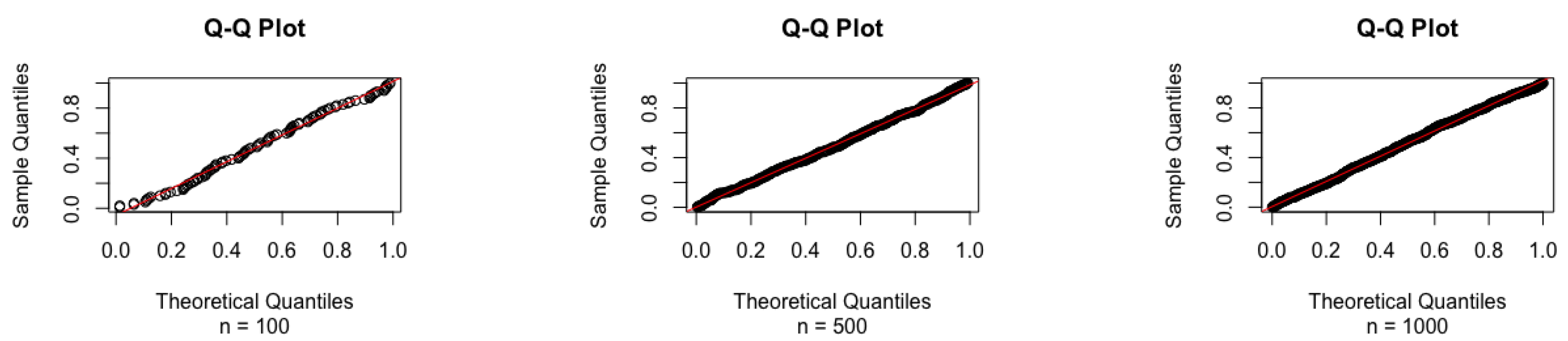
After following the steps above, we have successfully generated a random sample from the IGW distribution. However, we need to verify that the sample data are actually from the required IGW distribution. Thus, we make use of the standard approach via a quantile–quantile plot (Q-Q plot) to conduct the validation. This can be easily implemented in R using the function qqnorm(). However, there is no such function in R to draw a Q-Q plot using sample data from an IGW distribution. Hence, we carry out the following steps to create a Q-Q plot for comparing the sample data with an IGW distribution. Again, similar steps can be utilized to create a Q-Q plot for any other distributions, especially for the newly established ones.

• Step 1: generate a random sample of size n from IGW distribution, $X=(x_1,\dots ,x_n)$, using the method described above, $IGW(\alpha ,\beta ,\lambda )$.
• Step 2: Obtain the theoretical quantiles, say $T=(t_1,\dots ,t_n)$. Loop through each observation from the sample, X; for each $x_i$, obtain its theoretical quantile, $t_i$, using the density function of the specific $IGW(\alpha ,\beta ,\lambda )$ distribution. As an aside, note that the integrate() function in the statistical software R is very helpful in finding such quantiles. More specifically, $t_i=integrate(f(x,\alpha ,\beta ,\lambda ),0,x_i)$, where $i=1,\dots ,n$.
• Step 3: Find the sample quantiles, say $S=(s_1,\dots ,s_n)$. Here, $s_i$ is the ratio of the number of observations that are not greater than $x_i$ and sample size n.
• Step 4: plot the sample quantiles against the theoretical quantiles

From the plots given in Figure 1, we can see that the sample data indeed come from an IGW distribution, no matter whether the sample size is small (n = 100), medium (n = 500), or large (n = 1000).

In

Table 1. Simulation results when the sample data are simulated from IGW $(0.5,2,0.7)$ following the stopping rules in (16).

$\mathit{\delta }$	$\overline{\mathit{N}}$	${\mathit{n}}^{\ast }$	$\mathit{s}{\mathit{e}}_{\overline{\mathit{N}}}$	$\overline{\mathit{N}}/{\mathit{n}}^{\ast }$	${\mathit{R}}_{\mathit{N}}$	${\mathit{R}}_{\mathit{N}}/\mathit{\delta }$	$\overline{\widehat{\mathit{\alpha }}}$	$\mathit{s}{\mathit{e}}_{\overline{\overline{\widehat{\mathit{\alpha }}}}}$
0.006	50.725	48.777	0.113	1.040	0.005	0.871	0.497	0.001
0.003	92.923	90.830	0.168	1.023	0.003	0.932	0.498	0.001
0.002	135.267	132.648	0.301	1.020	0.002	0.965	0.500	0.001
0.001	261.575	257.815	0.434	1.015	0.001	0.974	0.501	0.000
0.0007	369.546	365.011	0.521	1.012	0.001	0.974	0.501	0.000
0.0005	512.516	507.905	1.402	1.009	0.000	1.003	0.501	0.001

,

Table 2. Simulation result when the sample data are simulated from IGW $(1,2,1)$ following the stopping rules in (16).

$\mathit{\delta }$	$\overline{\mathit{N}}$	${\mathit{n}}^{\ast }$	$\mathit{s}{\mathit{e}}_{\overline{\mathit{N}}}$	$\overline{\mathit{N}}/{\mathit{n}}^{\ast }$	${\mathit{R}}_{\mathit{N}}$	${\mathit{R}}_{\mathit{N}}/\mathit{\delta }$	$\overline{\widehat{\mathit{\alpha }}}$	$\mathit{s}{\mathit{e}}_{\overline{\overline{\widehat{\mathit{\alpha }}}}}$
0.02	55.697	54.289	0.129	1.026	0.018	0.893	0.988	0.001
0.01	105.557	104.388	0.190	1.011	0.010	0.954	0.992	0.001
0.008	130.686	129.409	0.214	1.010	0.008	0.957	0.994	0.001
0.005	205.916	204.442	0.276	1.007	0.005	0.976	0.996	0.001
0.002	506.565	504.476	0.440	1.004	0.002	0.976	0.999	0.000
0.001	1007.801	1004.488	0.630	1.003	0.001	0.993	1.000	0.000

,

Table 3. Simulation result when the sample data are simulated from IGW $(2,2,4)$ following the stopping rules in (16).

$\mathit{\delta }$	$\overline{\mathit{N}}$	${\mathit{n}}^{\ast }$	$\mathit{s}{\mathit{e}}_{\overline{\mathit{N}}}$	$\overline{\mathit{N}}/{\mathit{n}}^{\ast }$	${\mathit{R}}_{\mathit{N}}$	${\mathit{R}}_{\mathit{N}}/\mathit{\delta }$	$\overline{\widehat{\mathit{\alpha }}}$	$\mathit{s}{\mathit{e}}_{\overline{\overline{\widehat{\mathit{\alpha }}}}}$
0.1	44.021	42.685	0.118	1.031	0.093	0.930	1.965	0.003
0.05	83.933	82.716	0.173	1.015	0.049	0.980	1.979	0.002
0.04	104.078	102.723	0.196	1.013	0.040	1.000	1.984	0.002
0.02	203.574	202.736	0.277	1.004	0.020	1.000	1.990	0.001
0.01	403.393	402.743	0.397	1.002	0.010	1.000	1.994	0.001
0.008	503.275	502.744	0.440	1.001	0.008	1.000	1.995	0.001

,

Table 4. Simulation result when the sample data are simulated from IGW $(4,2,3)$ following the stopping rules in (16).

$\mathit{\delta }$	$\overline{\mathit{N}}$	${\mathit{n}}^{\ast }$	$\mathit{s}{\mathit{e}}_{\overline{\mathit{N}}}$	$\overline{\mathit{N}}/{\mathit{n}}^{\ast }$	${\mathit{R}}_{\mathit{N}}$	${\mathit{R}}_{\mathit{N}}/\mathit{\delta }$	$\overline{\widehat{\mathit{\alpha }}}$	$\mathit{s}{\mathit{e}}_{\overline{\overline{\widehat{\mathit{\alpha }}}}}$
0.1	163.049	161.872	0.252	1.007	0.102	1.020	3.975	0.003
0.05	323.060	321.873	0.358	1.004	0.051	1.020	3.989	0.002
0.04	403.029	401.874	0.397	1.003	0.040	1.000	3.992	0.002
0.02	802.248	801.874	0.564	1.000	0.020	1.000	3.995	0.001
0.01	1600.995	1601.875	0.799	0.999	0.010	1.000	3.997	0.001
0.008	2000.736	2001.875	0.890	0.999	0.008	1.000	3.997	0.001

and

Table 5. Simulation results when the sample data are simulated from IGW $(10,2,3)$ following the stopping rules in (16).

$\mathit{\delta }$	$\overline{\mathit{N}}$	${\mathit{n}}^{\ast }$	$\mathit{s}{\mathit{e}}_{\overline{\mathit{N}}}$	$\overline{\mathit{N}}/{\mathit{n}}^{\ast }$	${\mathit{R}}_{\mathit{N}}$	${\mathit{R}}_{\mathit{N}}/\mathit{\delta }$	$\overline{\widehat{\mathit{\alpha }}}$	$\mathit{s}{\mathit{e}}_{\overline{\overline{\widehat{\mathit{\alpha }}}}}$
1.500	68.916	68.019	0.169	1.013	1.768	1.117	9.828	0.013
1.200	85.162	84.685	0.186	1.006	1.359	1.085	9.840	0.012
0.900	113.015	112.462	0.216	1.005	0.997	1.072	9.885	0.010
0.500	201.991	201.351	0.280	1.003	0.501	0.985	9.941	0.007
0.300	335.972	334.684	0.367	1.004	0.307	1.011	9.973	0.006
0.100	1003.008	1001.350	0.622	1.002	0.097	0.964	9.993	0.003

, we summarized a number of selective simulation results. We included results from five different IGW distributions, IGW $(0.5,2,0.7)$, IGW $(1,2,1)$, IGW $(2,2,4)$, IGW $(4,2,3)$, and IGW $(10,2,3)$. From Figure 2, with five different parameter value combinations, we observe five distinct shapes of the IGW distribution. Thus, the simulation results from these five distributions would provide a solid double-validation in addition to the theoretical findings we provided in Theorems 1 and 2. Moreover, the preassigned risk upper bound, $\delta$, is chosen in order to show the results for small, moderate, and large sample sizes.

Sample data are simulated while exactly following the simulation procedure, as discussed in the first part of Section 3. The sampling procedure is implemented following the stopping rule, as per (16). For each simulation scenario, that is, for a given combination of parameter values, say $\alpha$,$\beta$, $\lambda$, and $\delta$, we replicate the whole process in order to obtain the average of the stopping variable, $\overline{N}$, as per (16). Also, we were able to calculate the standard error of $\overline{N}$. Additionally, estimated risk, ${\widehat{R}}_N$, can be calculated based on data upon termination, as per (24). The pilot sample size, m, was fixed to be 10 in each case (iteration). One may note that $\overline{N}$ should be close to the optimal sample size, $n^{\ast }$. ${\widehat{R}}_N$ should be close to the bounded-risk $\delta$. The last two columns of Table 1, Table 2, Table 3, Table 4 and Table 5 show the estimated $\alpha$ parameter averaged over 10,000 replicates and its standard errors.

The results consistently show the following: (1) the ratio of $\overline{N}$ and $n^{\ast }$ hangs around 1 with small standard errors, which doubly validates the properties in Theorem 1; (2) the ratio of the estimated risk, $R_N$, and the theoretical risk, $\delta$, is close to 1, which doubly validates the properties in Theorem 2.

Further, we highlight the simulation performance of our developed procedures of creating fixed-accuracy confidence intervals for $\alpha$. Interestingly, as seen earlier in (27), since the rule for determining the sample size does not depend on any of the unknown parameters, one need not attempt a sequential rule to obtain the optimal sample size, N. We, hence, adopt the following simple approach in order to obtain N, with only pre-fixed $\eta$ and d.

• Step 1: fix the constant d and the required confidence level $1-\eta$ (say $0.95,0.99$, etc.)
• Step 2: For every value of the possible optimal sample size, N, starting from 1, generate a single random observation from a gamma distribution with parameters N and $1/N$. Let this be denoted as T.
• Step 3: find $P\{d^{-1}<T<d\}$ for every value of N.
• Step 4: stop the process when $P\{d^{-1}<T<d\}$ exceeds $1-\eta$, which yields the final optimal sample size, N.

In

Table 6. Simulation results for the fixed-accuracy confidence interval when the sample data are simulated from IGW $(4,2,3)$ following the rule in (27) with $\eta =0.5$.

d	N	${\overline{\widehat{\mathit{\alpha }}}}_{\mathit{N}}$	c.p.
1.2	117	4.0332	0.9470
1.15	198	4.0188	0.9496
1.1	424	4.0130	0.9485
1.09	519	4.0089	0.9492
1.08	650	4.0054	0.9471
1.07	840	4.0073	0.9489

, we summarized the results from Section 2.2, which discusses the fixed-accuracy confidence interval estimation on the parameter $\alpha$. According to (27), the only parameters that affect the sample size would be the fixed-accuracy measurement d and the confidence level $1-\eta$. Table 6 includes the summarized results when the sample data are simulated from IGW $(4,2,3)$. For different values of d, with fixed $\eta =0.05$, following steps 1–4, we can determine the number of observations we need, which is shown in column 2 of Table 6. Clearly, if we fix d to be very small, one would require more samples to be able to meet the $100(1-\eta )\%$ level. We replicate the sampling procedure $10,000$ times to check on the performance of $\widehat{\alpha }$, as well as the coverage probability. As is seen from column 3, we listed the average of $10,000$ values of $\widehat{\alpha }$, which are all close to $\alpha =4$. Moreover, the last column showed us that the coverage probability, in all the cases, is close to the corresponding level, which was set to be $95\%$. It is worth mentioning that one does not need to know the values of the other two parameters, $\beta$ and $\lambda$, to create the desired confidence interval for $\alpha$.

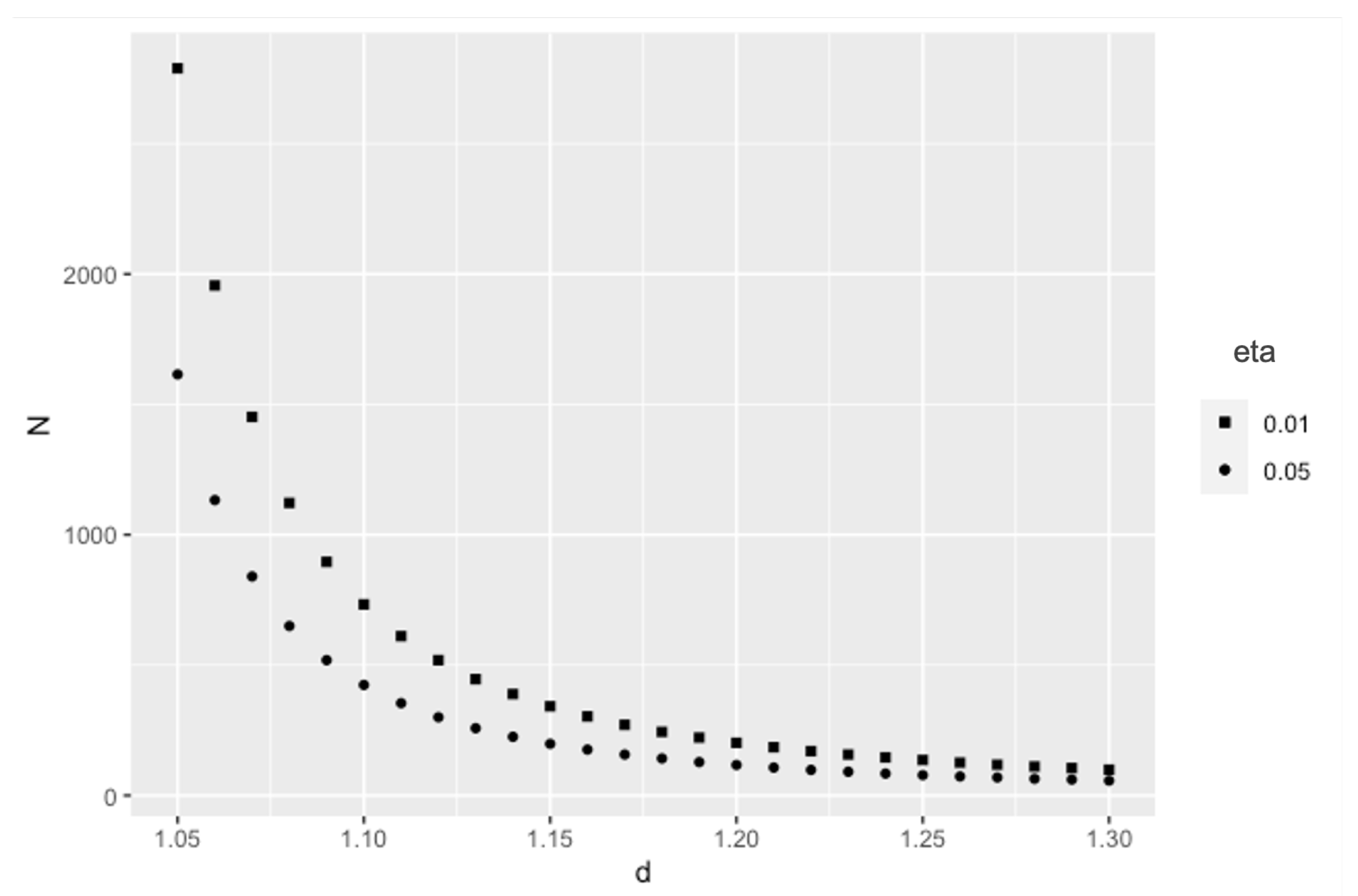
Further, Figure 3 shows the relationship between varying optimal sample sizes over a range of d values for fixed values of $\eta$. Clearly, as seen from the above table also, as d reduces, one would require more samples to still find the confidence interval at the $1-\eta$ level. This makes a lot of sense because a smaller d means a tighter confidence interval, and one needs more observations to achieve that tighter interval. Also, for the same d, a smaller $\eta$ means that a larger sample is required, due to a higher confidence level.

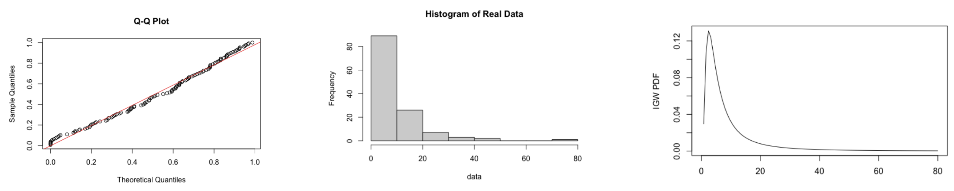
4. Real Data Applications

In this section, we apply the proposed methodologies to a couple of practical scenarios. The first set of data we consider is the remission time (in months) of 128 patients suffering from bladder cancer. This data set has been given wide attention. The original data were brought up by Ref. [28]. Ref. [29] discussed this data set using McDonald Lomax distribution. Ref. [30] used this data set on Marshall–Olkin generalized defective Gompertz distribution. Ref. [22] showed the adequacy of inverse generalized Weibull distribution in modeling this data through some goodness of fit measures such as AIC and BIC.

It is reasonable to assume that the remission times of bladder cancer patients follow an IGW distribution. Based on the given data for the 128 patients, as well as the information from [22], we further assume the distribution is IGW $(\alpha =61.38,\beta =0.51,\lambda =8.19)$. Figure 3 displays the Q-Q plot for the observed data versus the theoretical IGW distribution, given that $\alpha =61.38,\beta =0.51,\lambda =8.19$, which confirms that this data set would be suitable for the proposed methodologies. We have also included the histogram of the observed data, and the density curve, to provide further insight.

To start with, we randomize the original data set and pretend the patients’ data come in this randomized order.

Table 7. Randomly ordered remission data from 128 bladder cancer patients. The original data source is given [28].

3.36	9.74	7.09	7.59	1.4	4.23	8.66	25.74	6.97	3.02	2.83	19.13
3.82	12.07	3.48	1.76	32.15	25.82	2.62	2.64	5.71	5.41	10.66	4.51
8.26	3.7	2.02	17.36	14.77	0.5	7.32	3.25	7.66	7.63	5.32	7.28
7.87	6.25	1.26	23.63	5.32	5.09	21.73	79.05	2.54	8.37	26.31	5.17
11.25	13.29	3.57	3.52	7.62	2.87	2.69	2.09	10.34	15.96	18.1	6.94
1.35	1.05	4.4	4.26	17.12	12.02	36.66	0.4	2.26	2.69	0.9	8.65
20.28	5.85	7.39	43.01	0.2	12.03	11.98	7.93	8.53	6.93	2.46	14.24
5.41	9.02	9.22	5.49	17.14	2.23	14.76	46.12	3.36	13.8	5.06	6.76
4.87	9.47	4.5	0.51	11.79	4.33	5.34	1.19	22.69	3.31	10.75	13.11
11.64	7.26	3.88	2.02	4.18	4.34	34.26	5.62	1.46	0.08	0.81	10.06
2.07	4.98	16.62	14.83	6.54	3.64	12.63	2.75

is a copy of the randomized data records.

We then further set $\delta =0.08$. Now, as per (16), we implement the sequential sampling procedure. We start with the first two observations and then continue taking one observation at a time, according to Table 5. The sampling procedure is terminated at the 76th record. That is, in real-life situations, if we are collecting the data and waiting to get an estimation for $\alpha$, we would only require 76 observations. And there is no need to continue sampling, which would, for sure, waste time and money. Upon termination, the estimated $\alpha$ is $60.09$, which is a close estimation of $61.38$ that is assumed to be the population shape parameter. Again, the stopping rule (16) was created based on an upper estimation risk bound, and we set it to be $0.08$ in this case.

Now, using this real data set, we illustrate the procedures we discussed for constructing a fixed-accuracy confidence interval for $\alpha$.

Suppose a group of researchers has decided to create a $95\%$ confidence interval for $\alpha$ with $d=1.2$. According to (27), we search for the sample size that is needed under such requirements. The smallest sample size that is needed turns out to be 73. Figure 4 shows the relationship between the coverage probability and the required sample size, as per (27). It is clear that, as we increase the sample size N, the coverage probability goes up for fixed values of d and $\eta$. Thus, sample size 73 is the minimum number of observations that we need to achieve the targeted level, $95\%$.

Now, using the data that we set up from Table 5, we just take the first 73 observations and construct the confidence interval for $\alpha$. These observations give us a $95\%$ confidence interval as $(59.84.11,63.07)$. This interval covers the true value of $\alpha$, which is $61.38$, by only utilizing 73 observations.

We will now work with the second data set and try to put forward a similar approach to finding the fixed accuracy confidence interval for $\alpha$, as was conducted for the first one. This data set contains waiting times (in minutes) before access to customer service at 100 banks. The data set can be found to have been analyzed in [31], where the author fitted Lindley distribution to the data. However, the applicability of an IGW distribution can be seen in [22]. It is reasonable to assume that the waiting times follow an IGW distribution. Based on the given data, and the information given in [22], we further confirm the distribution as IGW $(\alpha =40.73,\beta =0.77,\lambda =8.55)$. As before, we first randomize the entire data set and pretend the data come from this randomized order.

Table 8. Randomly ordered waiting-time data from 100 banks. The original data source is given [31].

2.9	21.3	9.8	8.0	3.3	8.8	21.4	31.6	5.7	9.6
7.6	4.2	6.9	1.5	13.6	8.6	21.9	11.5	9.7	8.2
17.3	4.8	7.1	1.9	4.0	18.1	3.1	11.1	15.4	4.9
11.2	1.9	3.6	4.7	13.0	7.1	7.4	13.1	2.6	3.5
5.7	8.9	5.0	12.9	10.7	13.9	4.9	23.0	6.3	6.7
9.5	10.9	19.0	6.2	4.3	4.2	5.3	19.9	18.4	5.5
6.1	7.7	2.7	4.3	15.4	3.2	11.0	11.0	4.4	38.5
8.6	11.2	0.8	11.9	17.3	8.6	13.3	33.1	14.1	1.3
1.8	4.6	6.2	7.1	2.1	20.6	12.4	18.9	4.7	12.5
4.1	6.2	18.2	8.9	4.4	8.8	27.0	0.8	13.7	7.1

is a copy of the randomized data for reference.

Now suppose one needs to create a $95\%$ confidence interval for $\alpha$ with $d=1.2$. According to (27), we search for the sample size that is needed under such requirements. The smallest sample size that is needed turns out to be 58. Again, it can be shown that, as we increase the sample size, N, the coverage probability goes up, for fixed values of d and $\eta$. Thus, sample size 58 is the minimum number of observations that we need to achieve the targeted level, $95\%$.

Now, using the data that we set up from Table 6, we just take the first 58 observations and construct the confidence interval for $\alpha$. These observations give us a $95\%$ confidence interval as $(39.11,42.72)$. This interval covers the true value of $\alpha$, which is $40.73$, by only utilizing 58 observations.

5. Conclusions

In this paper, we developed two methodologies for statistical inference of the shape parameter of the inverse generalized Weibull distribution (IGW). IGW distribution involves three parameters, $\alpha$, $\beta$, and $\lambda$. The first methodology is created to build a bounded-risk point estimator of $\alpha$ when both $\beta$ and $\lambda$ are known. For this, we developed a purely sequential procedure to determine the optimal sample size, when the estimation risk is bounded by a pre-assigned value. The purely sequential rules enjoy a number of appealing properties, which were proved in theorems, as well as validated via simulation studies. The second methodology is for constructing a fixed-accuracy confidence interval for $\alpha$. For this, one is not required to have any knowledge of the other two parameters, $\beta$ and $\lambda$, in order to decide on the desired sample size. The sample size can be determined directly for any given confidence level $100(1-\eta )\%$ and pre-fixed accuracy parameter, d.

Simulations on many traditional distributions are very easy using the statistical software R. However, the simulation for the IGW distribution is not as straightforward. Using the rejection sampling technique, we designed a detailed procedure for simulating sample data from any given distribution, regardless of its complexity. This also enabled us to conduct simulation studies and illustrate the real-world application of the newly designed methodologies.

An important consideration is how to choose appropriate parameter values, such as the risk bound $\delta$ or the fixed-accuracy measure d. For bounded-risk point estimation, one needs to set up an upper bound ($\delta$) for the risk on estimating the parameter $\alpha$. There is no golden rule on deciding the value of $\delta$. Historical data may help if one can obtain any helpful historical data. Moreover, the cost of sampling and the time required to obtain sample data in different situations can also affect the decision. If one wants to have a general estimation of $\alpha$, they may fix $\delta$ at a higher value so that fewer observations are needed. If one requires higher accuracy, then $\delta$ may be set up to a much smaller number. Similarly, for fixed-accuracy confidence interval estimations, one needs to decide on the values of d and $\eta$ based on specific problems. Again, a tighter confidence interval means a smaller d and it requires more sample observations; a higher confidence level means a smaller $\eta$, and it requires a larger sample size.

Generalized Weibull distributions take many different forms with different numbers of parameters. Its flexibility allows its wide use in real-life problems. In the future, we will try to work on estimating all three parameters involved in this inverse generalized Weibull distribution with a minimal required sample since people may not have any prior knowledge of any of the parameters. For brevity, we want to bring up an idea using an iterative estimation approach to estimate all parameters. (1) Begin with a small pilot sample of observations from the population, say $n_0$. In this initial step, set $\alpha =1$ to simplify the estimation of $\beta$ and $\lambda$. Using this pilot sample, estimate $\beta$ and $\lambda$ through the MLE method. Let these initial estimates be denoted as ${\widehat{\beta }}_0$ and ${\widehat{\lambda }}_0$. (2) Using the initial estimates ${\widehat{\beta }}_0$ and ${\widehat{\lambda }}_0$, obtain the initial estimate for $\alpha$. Following the stopping rule we developed on bounded-risk point estimation, we will take one more observation at a time. As new observations are sequentially added, re-estimate $\alpha$ with the most recent values of $\beta$ and $\lambda$; then, update $\beta$ and $\lambda$ based on the new $\alpha$ estimate. This iterative procedure is repeated until the stopping criterion is met for $\alpha$. (3) Once the stopping criterion is met, the current estimates of $\alpha$, $\beta$, and $\lambda$ are taken as the final estimates. Similarly, for the fixed-accuracy confidence interval estimation, using the determined sample size, one can achieve MLE for $\beta$ and $\lambda$ first and then obtain the confidence interval for $\alpha$.