Analytical Valuation of Vulnerable Exchange Options with Stochastic Volatility in a Reduced-Form Model

Abstract

This paper investigates the valuation of vulnerable exchange options with two underlying assets that follow a two-factor volatility model. We employ a reduced-form model incorporating a Poisson process with stochastic intensity. The proposed reduced-form model depends on a stochastic intensity process that is guaranteed to remain positive and includes both systemic and idiosyncratic risks. Using measure change techniques and characteristic functions, we obtain an explicit pricing formula for vulnerable exchange options within the proposed framework. We also provide numerical examples demonstrating the sensitivity of option prices to significant parameters.

1. Introduction

The valuation of options that consider counterparty credit risk, termed ‘vulnerable options’, has received significant attention from numerous researchers. Vulnerable options are financial derivatives that incorporate the credit risk associated with the counterparty’s potential default. The adoption of a credit risk model is required to accurately evaluate vulnerable options. In general, two main approaches have been used for modeling credit risk: the structural model and the reduced-form model. The structural model, pioneered by Merton [1] and Black and Cox [2], links credit events to the firm’s value process. A credit event occurs when the firm’s value falls below its liabilities at maturity. In contrast, the reduced-form model, initially developed by Jarrow and Turnbull [3] and Jarrow and Yu [4], separates credit events from the firm’s value. Instead, a credit event is initiated by the first jump of a Poisson process with a predetermined intensity, independent of the firm’s value dynamics. This paper is in line with the development of the reduced-form model.

We employ a reduced-form model to explore the pricing of vulnerable options. Recent studies have focused on vulnerable options within reduced-form model frameworks. Fard [5] developed a pricing formula for vulnerable options under a generalized jump model, utilizing a reduced-form approach to describe counterparty credit risk. Pasricha and Goel [6] investigated a vulnerable power exchange option with two underlying assets within a reduced-form framework. They employed a doubly stochastic Poisson process to model counterparty credit events and incorporated correlations among the three assets in both continuous and jump components. Wang [7] considered basket warrants with default risk under a stochastic volatility model. In addition, Wang [8,9] studied the valuation of European options, Asian options, and fader options with default risk and stochastic volatility in a reduced-form model. More recently, under reduced-form models, Pan et al. [10] provided the pricing formula of European options with default risk in a market where the underlying stocks are not perfectly liquid, and Wang et al. [11] investigated the pricing problem of vulnerable basket options with stochastic liquidity risk. This paper also considers the vulnerable option under a stochastic volatility model. Specifically, vulnerable exchange options, which have two underlying assets, with stochastic volatility are investigated through a reduced-form model.

The aim of this paper is to provide an explicit solution for vulnerable exchange option pricing. In fact, there have been several studies on vulnerable exchange options. Pasricha and Goel [6] developed a vulnerable exchange option pricing model based on correlated dynamics in both the continuous and jump parts. In [12], vulnerable exchange options with early default risk were studied employing dimension reduction, Mellin transform, and the method of images. In addition, the valuation of vulnerable exchange options with the stochastic volatility was investigated in the structural model [13,14]. Unlike prior studies, we apply a reduced-form model in continuous time and two-factor stochastic volatility to demonstrate the credit risk model and the underlying assets, respectively. Furthermore, by dividing the risk into idiosyncratic and systematic components, we complete the reduced-form model. In the proposed model, we derive an explicit pricing formula for vulnerable exchange options.

The remainder of this paper is organized as follows. In Section 2, we introduce the model dynamics, and the pricing problem for vulnerable exchange options is formulated. In Section 3, we derive the explicit solution for option pricing in terms of a characteristic function using the measure change technique. In Section 4, we provide numerical examples to show various characteristics of options with respect to significant parameters. Finally, Section 5 offers concluding remarks.

2. Model

Let $(\mathsf{\Omega },\mathcal{F},Q)$ be a filtered probability space satisfying the usual conditions, where Q is a risk-neutral measure. We assume that the underlying assets $S_1\left(t\right)$ and $S_2\left(t\right)$, which are associated, respectively, with a two-factor stochastic volatility model as described in Christoffersen et al. [15], are governed by the following processes:

$$\begin{gathered} \frac{d{S}_1\left(t\right)}{S_1\left(t\right)}=rdt+{\beta }_1\sqrt{v_1\left(t\right)}d{W}_1\left(t\right)+\sqrt{v_2\left(t\right)}d{W}_2\left(t\right), \\ \frac{d{S}_2\left(t\right)}{S_2\left(t\right)}=rdt+{\beta }_2\sqrt{v_1\left(t\right)}d{W}_1\left(t\right)+\sqrt{v_3\left(t\right)}d{W}_3\left(t\right), \end{gathered}$$

(1)

where r is the interest rate, ${\beta }_i$$(i=1,2)$, which capture the sensitivities of underlying assets to systematic risk, are constants, $W_i\left(t\right)$$(i=1,2)$ are standard Brownian motions, and

$$\begin{array}{c}\hfill d{v}_i\left(t\right)=(a_i-b_i{v}_i\left(t\right))dt+{\gamma }_i\sqrt{v_i\left(t\right)}d{B}_i\left(t\right),(i=1,2,3)\end{array}$$

(2)

where $a_i,b_i,{\gamma }_i$$(i=1,2,3)$ are constants, and $B_i\left(t\right)$$(i=1,2,3)$ are the correlated standard Brownian motions satisfying $d{W}_1\left(t\right)d{B}_1\left(t\right)={\rho }_{1}dt,d{W}_2\left(t\right)d{B}_2\left(t\right)={\rho }_{2}dt,$ and $d{W}_3\left(t\right)d{B}_3\left(t\right)={\rho }_{3}dt$, and other Brownian motions are pairwise independent.

In what follows, we model the credit risk of an option issuer using a reduced form model. Following Wang [8], the intensity process is divided into two parts. The first part addresses the systematic risk, while the second part addresses the idiosyncratic risk of option issuers. In more detail, in the work of Wang [8], we can find that $v_1\left(t\right)$ means the variance of the market portfolio corresponding to systematic risk, $v_2\left(t\right)$ means the variance corresponding to idiosyncratic risk of the underlying asset $S_1\left(t\right)$, and $v_3\left(t\right)$ means the variance corresponding to idiosyncratic risk of the underlying asset $S_2\left(t\right)$, respectively. Therefore, we assume that the intensity process is driven by the following process:

$$\lambda \left(t\right)=\beta v_1\left(t\right)+v\left(t\right),$$

where $\beta$ is is a nonnegative constant that captures the correlation between the process $v_1\left(t\right)$ and the process $\lambda \left(t\right)$. In addition, $v\left(t\right)$, which describes the idiosyncratic risk, is given by

$$\begin{array}{c}\hfill dv\left(t\right)=(a-bv\left(t\right))dt+\gamma \sqrt{v\left(t\right)}dB\left(t\right),\end{array}$$

(3)

where $a,b,\gamma$ are constants and $B\left(t\right)$ is a standard Brownian motion that is independent of the other Brownian motions. Given the intensity process $\lambda \left(t\right)$, the default $\tau$ is defined as

$$\mathrm{P}\left(\tau >t\right)=\mathrm{E}\left[e^{-{\int }_0^t\lambda \left(s\right)ds}\right],$$

where $t\in [0,T]$ and T is the maturity of an option.

In the reduced form model, we investigate a vulnerable exchange option with maturity T. Basically, the price of the option is determined by whether default occurs or not before maturity. In other words, if $\tau >T$, there is no default before the maturity, and if $0<\tau \le T$, the price is determined by the recover rate w. Then, we can find that the pricing expression includes two parts. From the assumptions, the price of the vulnerable exchange option at time 0 under the risk neutral measure Q can be presented as

$$\begin{array}{ccc}\hfill C& =& e^{-rT}{\mathrm{E}}^Q\left[{(S_1\left(T\right)-S_2\left(T\right))}^{+}{\mathbf{1}}_{\{\tau >T\}}+w{(S_1\left(T\right)-S_2\left(T\right))}^{+}{\mathbf{1}}_{\{\tau \le T\}}\right]\hfill \\ & =& (1-w)e^{-rT}{\mathrm{E}}^Q\left[{(S_1\left(T\right)-S_2\left(T\right))}^{+}{\mathbf{1}}_{\{\tau >T\}}\right]+w{e}^{-rT}{\mathrm{E}}^Q\left[{(S_1\left(T\right)-S_2\left(T\right))}^{+}\right],\hfill \end{array}$$

(4)

where w is the recovery rate satisfying $0<w\le 1$, and ${\mathrm{E}}^Q\left[·\right]$ is the expectation under the risk neutral measure Q.

3. Valuation of Vulnerable Exchange Option

In this section, we provide an analytic pricing formula of a vulnerable exchange option in the proposed framework. To derive the pricing formula of the option in (4), we need to define the joint characteristic function $f(\varphi ,{\varphi }_2,{\varphi }_3)$ of $(\ln S_1\left(T\right),\ln S_1\left(T\right),{\int }_0^T\lambda \left(s\right)ds)$ under the measure Q. That is, the function $f(\varphi ,{\varphi }_2,{\varphi }_3)$ is defined as

$$\begin{array}{c}\hfill f({\varphi }_1,{\varphi }_2,{\varphi }_3)={\mathrm{E}}^Q\left[e^{{\varphi }_1\ln S_1\left(T\right)+{\varphi }_2\ln S_2\left(T\right)+{\varphi }_3{\int }_0^T\lambda \left(s\right)ds}\right],\end{array}$$

(5)

where ${\varphi }_i(i=1,2,3)$ are complex numbers. To provide the explicit solution of the function $f(\varphi ,{\varphi }_2,{\varphi }_3)$, we should introduce the following lemma. For more details, one can refer to Cox et al. [16].

Lemma 1. 

For any complex numbers $s_1$ and $s_2$, the joint characteristic function of $({\int }_t^{T}v\left(s\right)ds,v\left(T\right))$ is given by

$$\begin{array}{ccc}\hfill P(s_1,s_2;t,T,v)& =& \mathrm{E}\left[e^{s_1{\int }_t^{T}v\left(s\right)ds+s_{2}v\left(T\right)}|v\left(t\right)=v\right]\hfill \\ & =& e^{A(s_1,s_2;t,T)-B(s_1,s_2;t,T)v}\hfill \end{array}$$

(6)

where $v\left(t\right)$ is defined in (3), $0\le t\le T$ and

$$\begin{array}{c}A(s_1,s_2;t,T)=\frac{2a}{{\gamma }^2}\ln \left(\frac{2m\left(s_1\right)e^{(m\left(s_1\right)+b\left)\right(T-t)/2}}{(m\left(s_1\right)+b-{\gamma }^2{s}_2)(e^{m\left(s_1\right)(T-t)}-1)+2m\left(s_1\right)}\right),\hfill \\ m\left(s_1\right)=\sqrt{b^2-2{\gamma }^2{s}_1},\hfill \\ B(s_1,s_2;t,T)=\frac{2s_1(1-e^{m\left(s_1\right)(T-t)})-u_2\left(2m\left(s_1\right)+(m\left(s_1\right)-b)(e^{m\left(s_1\right)(T-t)}-1)\right)}{(m\left(s_1\right)+b-s_2{\gamma }^2)(e^{m\left(s_1\right)(T-t)}-1)+2m\left(s_1\right)}.\hfill \end{array}$$

Applying the result in Lemma 1, we can find the explicit solution of the function $f({\varphi }_1,{\varphi }_2,{\varphi }_3)$ in the following Theorem.

Theorem 1. 

Under the risk-neutral measure Q, the joint characteristic function $f({\varphi }_1,{\varphi }_2,{\varphi }_3)$ defined in (5) is given by

$$\begin{array}{c}f({\varphi }_1,{\varphi }_2,{\varphi }_3)=\exp \left[A_1+A_2+A_3+A_4-B_1{v}_1\left(0\right)-B_2{v}_2\left(0\right)-B_3{v}_3\left(0\right)-B_{4}v\left(0\right)+G\right]\hfill \end{array}$$

where

$$\begin{array}{c}{A}_1={\displaystyle \frac{2a_1}{{\gamma }_1^2}}\ln \left({\displaystyle \frac{2m_1{e}^{\frac{1}{2}(m_1+b_1)T}}{(m_1+b_1-{\gamma }_1^2{d}_1)(e^{m_{1}T}-1)+2m_1}}\right),\hfill \\ B_1={\displaystyle \frac{2c_1(1-e^{m_{1}T})-d_1(2m_1+(m_1-b_1)(e^{m_{1}T}-1))}{(m_1+b_1-d_1{\gamma }_1^2)(e^{m_{1}T}-1)+2m_1}},\hfill \\ A_2={\displaystyle \frac{2a_2}{{\gamma }_2^2}}\ln \left({\displaystyle \frac{2m_2{e}^{\frac{1}{2}(m_2+b_2)T}}{(m_2+b_2-{\gamma }_2^2{d}_2)(e^{m_{2}T}-1)+2m_2}}\right),\hfill \\ B_2={\displaystyle \frac{2c_2(1-e^{m_{2}T})-d_2(2m_2+(m_2-b_2)(e^{m_2}-1))}{(m_2+b_2-d_2{\gamma }_2^2)(e^{m_{2}T}-1)+2m_2}},\hfill \\ A_3={\displaystyle \frac{2a_3}{{\gamma }_3^2}}\ln \left({\displaystyle \frac{2m_3{e}^{\frac{1}{2}(m_3+b_3)T}}{(m_3+b_3-d_3{\gamma }_3^2)(e^{m_{3}T}-1)+2m_3}}\right),\hfill \\ B_3={\displaystyle \frac{2c_3(1-e^{m_{3}T})-d_3(2m_3+(m_3-b_3)(e^{m_{3}T}-1))}{(m_3+b_3-d_3{\gamma }_3^2)(e^{m_{3}T}-1)+2m_3}},\hfill \\ A_4={\displaystyle \frac{2a}{{\gamma }^2}}\ln \left({\displaystyle \frac{2m_4{e}^{\frac{1}{2}(m_4+b)T}}{(m_4+b)(e^{m_{4}T}-1)+2m_4}}\right),\hfill \\ B_4={\displaystyle \frac{2{\varphi }_3(1-e^{m_{4}T})}{(m_4+b)(e^{m_{4}T}-1)+2m_4}},\hfill \\ m_1=\sqrt{b_1^2-2{\gamma }_1^2{c}_1},m_2=\sqrt{b_2^2-2{\gamma }_2^2{c}_2},m_3=\sqrt{b_3^2-2{\gamma }_3^2{c}_3},m_4=\sqrt{b^2-2{\gamma }^2{\varphi }_3}\hfill \\ G={\varphi }_1\left(\ln S_1\left(0\right)+rT-{\displaystyle \frac{{\rho }_1{\beta }_1}{{\gamma }_1}}(v_1\left(0\right)+a_{1}T)-{\displaystyle \frac{{\rho }_2}{{\gamma }_2}}(v_2\left(0\right)+a_{2}T)\right),\hfill \\ +{\varphi }_2\left(\ln S_2\left(0\right)+rT-{\displaystyle \frac{{\rho }_1{\beta }_2}{{\gamma }_1}}(v_1\left(0\right)+a_{1}T)-{\displaystyle \frac{{\rho }_3}{{\gamma }_3}}(v_3\left(0\right)+a_{3}T)\right),\hfill \\ c_1=\left[{\displaystyle \frac{{\rho }_1{b}_1({\varphi }_1{\beta }_1+{\varphi }_2{\beta }_2)}{{\gamma }_1}}+{\displaystyle \frac{1}{2}}\left({({\varphi }_1{\beta }_1+{\varphi }_2{\beta }_2)}^2(1-{\rho }_1^2)-{\varphi }_1{\beta }_1^2-{\varphi }_2{\beta }_2^2+2{\varphi }_3\beta \right)\right],\hfill \\ d_1={\displaystyle \frac{{\rho }_1}{{\gamma }_1}}({\varphi }_1{\beta }_1+{\varphi }_2{\beta }_2),c_2={\displaystyle \frac{{\varphi }_1{\rho }_2{b}_2}{{\gamma }_2}}+{\displaystyle \frac{{\varphi }_1}{2}}({\varphi }_1(1-{\rho }_2^2)-1),d_2={\displaystyle \frac{{\varphi }_1{\rho }_2}{{\gamma }_2}},\hfill \\ c_3={\displaystyle \frac{{\varphi }_2{\rho }_3{b}_3}{{\gamma }_3}}+{\displaystyle \frac{{\varphi }_2}{2}}({\varphi }_2(1-{\rho }_3^2)-1),d_3={\displaystyle \frac{{\varphi }_2{\rho }_3}{{\gamma }_3}}.\hfill \end{array}$$

Proof. 

We consider the dynamics of underlying asset s $S_1\left(T\right)$ and $S_2\left(T\right)$ in (1). Then, $\ln S_1\left(T\right)$ and $\ln S_2\left(T\right)$ are presented as

$$\begin{array}{c}\ln S_1\left(T\right)=\ln S_1\left(0\right)+rT-\frac{1}{2}\left({\beta }_1^2{\int }_0^T{v}_1\left(u\right)du+{\int }_0^T{v}_2\left(u\right)du\right)\hfill \\ +{\beta }_1{\int }_0^T\sqrt{v_1\left(u\right)}d{W}_1\left(u\right)+{\int }_0^T\sqrt{v_2\left(u\right)}d{W}_2\left(u\right),\hfill \\ \ln S_2\left(T\right)=\ln S_2\left(0\right)+rT-\frac{1}{2}\left({\beta }_2^2{\int }_0^T{v}_1\left(u\right)du+{\int }_0^T{v}_3\left(u\right)du\right)\hfill \\ +{\beta }_2{\int }_0^T\sqrt{v_1\left(u\right)}d{W}_1\left(u\right)+{\int }_0^T\sqrt{v_3\left(u\right)}d{W}_3\left(u\right).\hfill \end{array}$$

(7)

Based on the above expression, we rewrite $\ln S_1\left(T\right)$ and $\ln S_2\left(T\right)$ as

$$\begin{array}{c}\ln S_1\left(T\right)=\ln S\left(0\right)+rT-{\displaystyle \frac{{\beta }_1{\rho }_1}{{\gamma }_1}}(v_1\left(0\right)-v_1\left(T\right)+a_{1}T)-{\displaystyle \frac{{\rho }_2}{{\gamma }_2}}(v_2\left(0\right)-v_2\left(T\right)+a_{2}T)\hfill \\ +\left({\displaystyle \frac{{\beta }_1{\rho }_1{b}_1}{{\gamma }_1}}-{\displaystyle \frac{{\beta }_1^2}{2}}\right){\int }_0^T{v}_1\left(u\right)du+\left({\displaystyle \frac{{\rho }_2{b}_2}{{\gamma }_2}}-{\displaystyle \frac{1}{2}}\right){\int }_0^T{v}_2\left(u\right)du\hfill \\ +\sqrt{1-{\rho }_2^2}{\int }_0^T\sqrt{v_2\left(u\right)}\widetilde{W_2}\left(u\right)+{\beta }_1\sqrt{1-{\rho }_1^2}{\int }_0^T\sqrt{v_1\left(u\right)}\widetilde{W_1}\left(u\right),\hfill \\ \ln S_2\left(T\right)=\ln S_2\left(0\right)+rT-{\displaystyle \frac{{\beta }_2{\rho }_1}{{\gamma }_1}}(v_1\left(0\right)-v_1\left(T\right)+a_{1}T)-{\displaystyle \frac{{\rho }_3}{{\gamma }_3}}(v_3\left(0\right)-v_3\left(T\right)+a_{3}T)\hfill \\ +\left({\displaystyle \frac{{\rho }_3{b}_3}{{\gamma }_3}}-{\displaystyle \frac{1}{2}}\right){\int }_0^T{v}_3\left(u\right)du+\left({\displaystyle \frac{{\beta }_2{\rho }_1{b}_1}{{\gamma }_1}}-{\displaystyle \frac{{\beta }_2^2}{2}}\right){\int }_0^T{v}_1\left(u\right)du\hfill \\ +\sqrt{1-{\rho }_3^2}{\int }_0^T\sqrt{v_3\left(u\right)}\widetilde{W_3}\left(u\right)+{\beta }_2\sqrt{1-{\rho }_1^2}{\int }_0^T\sqrt{v_1\left(u\right)}\widetilde{W_1}\left(u\right),\hfill \end{array}$$

(8)

where $\widetilde{W_1}\left(t\right)$ and $\widetilde{W_2}\left(t\right)$ are the standard Brownian motions, and are independent of other Brownian motions. These have the following forms:

$$W_1\left(t\right)={\rho }_1{B}_1\left(t\right)+\sqrt{1-{\rho }_1^2}\widetilde{W_1}\left(t\right),W_2\left(t\right)={\rho }_2{B}_2\left(t\right)+\sqrt{1-{\rho }_2^2}\widetilde{W_2}\left(t\right),$$

respectively. Adding (8) in (5), the function $f({\varphi }_1,{\varphi }_2,{\varphi }_3)$ is represented as

$$\begin{array}{c}f({\varphi }_1,{\varphi }_2,{\varphi }_3)={\mathrm{E}}^Q\left[e^{{\varphi }_1\ln S_1\left(T\right)+{\varphi }_2\ln S_2\left(T\right)+{\varphi }_3{\int }_0^T\lambda \left(s\right)ds}\right]\hfill \\ ={\mathrm{E}}^Q\left[\exp \left\{\left({\displaystyle \frac{{\rho }_1{b}_1({\varphi }_1{\beta }_1+{\varphi }_2{\beta }_2)}{{\gamma }_1}}-{\displaystyle \frac{1}{2}}({\varphi }_1{\beta }_1^2+{\varphi }_2{\beta }_2^2-2{\varphi }_3\beta )\right){\int }_0^T{v}_1\left(s\right)ds\right.\right.\hfill \\ \left.\left.+{\displaystyle \frac{{\rho }_1}{{\gamma }_1}}({\varphi }_1{\beta }_1+{\varphi }_2{\beta }_2)v_1\left(T\right)+({\varphi }_1{\beta }_1+{\varphi }_2{\beta }_2)\sqrt{1-{\rho }_1^2}{\int }_0^T\sqrt{v_1\left(s\right)}d\widetilde{W_1}\left(s\right)\right\}\right]\hfill \\ \times {\mathrm{E}}^Q\left[\exp \left\{{\displaystyle \frac{{\varphi }_1{\rho }_2}{{\gamma }_2}}{v}_2\left(T\right)+{\varphi }_1\left({\displaystyle \frac{{\rho }_2{b}_2}{{\gamma }_2}}-{\displaystyle \frac{1}{2}}\right){\int }_0^T{v}_2\left(s\right)ds+{\varphi }_1\sqrt{1-{\rho }_2^2}{\int }_0^T\sqrt{v_2\left(s\right)}\widetilde{W_2}\left(s\right)\right\}\right]\hfill \\ \times {\mathrm{E}}^Q\left[\exp \left\{{\displaystyle \frac{{\varphi }_2{\rho }_3}{{\gamma }_3}}{v}_3\left(T\right)+{\varphi }_2\left({\displaystyle \frac{{\rho }_3{b}_3}{{\gamma }_3}}-{\displaystyle \frac{1}{2}}\right){\int }_0^T{v}_3\left(s\right)ds+{\varphi }_2\sqrt{1-{\rho }_3^2}{\int }_0^T\sqrt{v_3\left(s\right)}\widetilde{W_3}\left(s\right)\right\}\right]\hfill \\ \times {\mathrm{E}}^Q\left[e^{{\varphi }_3{\int }_0^{T}v\left(s\right)ds}\right]\times e^G.\hfill \end{array}$$

(9)

We deal with the first expectation in (9). To obtain the explicit solution, we apply the law of iterated expectation. Then, we have that

$$\begin{array}{c}{\mathrm{E}}^Q\left[\exp \left\{\left({\displaystyle \frac{{\rho }_1{b}_1({\varphi }_1{\beta }_1+{\varphi }_2{\beta }_2)}{{\gamma }_1}}-{\displaystyle \frac{1}{2}}({\varphi }_1{\beta }_1^2+{\varphi }_2{\beta }_2^2-2{\varphi }_3\beta )\right){\int }_0^T{v}_1\left(s\right)ds\right.\right.\hfill \\ \left.\left.+{\displaystyle \frac{{\rho }_1}{{\gamma }_1}}({\varphi }_1{\beta }_1+{\varphi }_2{\beta }_2)v_1\left(T\right)+({\varphi }_1{\beta }_1+{\varphi }_2{\beta }_2)\sqrt{1-{\rho }_1^2}{\int }_0^T\sqrt{v_1\left(s\right)}d\widetilde{W_1}\left(s\right)\right\}\right]\hfill \\ ={\mathrm{E}}^Q\left[\exp \left\{\left({\displaystyle \frac{{\rho }_1{b}_1({\varphi }_1{\beta }_1+{\varphi }_2{\beta }_2)}{{\gamma }_1}}-{\displaystyle \frac{1}{2}}({\varphi }_1{\beta }_1^2+{\varphi }_2{\beta }_2^2-2{\varphi }_3\beta )\right){\int }_0^T{v}_1\left(s\right)ds\right.\right.\hfill \\ \left.+{\displaystyle \frac{{\rho }_1}{{\gamma }_1}}({\varphi }_1{\beta }_1+{\varphi }_2{\beta }_2)v_1\left(T\right)\right\}\times \left.{\mathrm{E}}^Q\left[\exp \left\{({\varphi }_1{\beta }_1+{\varphi }_2{\beta }_2)\sqrt{1-{\rho }_1^2}{\int }_0^T\sqrt{v_1\left(s\right)}d\widetilde{W_1}\left(s\right)\right\}|{\mathcal{F}}_T\right]\right]\hfill \end{array}$$

$$\begin{array}{c}={\mathrm{E}}^Q\left[\exp \left\{\left({\displaystyle \frac{{\rho }_1{b}_1({\varphi }_1{\beta }_1+{\varphi }_2{\beta }_2)}{{\gamma }_1}}-{\displaystyle \frac{1}{2}}({\varphi }_1{\beta }_1^2+{\varphi }_2{\beta }_2^2-2{\varphi }_3\beta )\right){\int }_0^T{v}_1\left(s\right)ds\right.\right.\hfill \\ \left.\left.+{\displaystyle \frac{{\rho }_1}{{\gamma }_1}}({\varphi }_1{\beta }_1+{\varphi }_2{\beta }_2)v_1\left(T\right)\right\}\exp \left\{{\displaystyle \frac{{({\varphi }_1{\beta }_1+{\varphi }_2{\beta }_2)}^2(1-{\rho }_1^2)}{2}}{\int }_0^T{v}_1\left(s\right)ds\right\}\right]\hfill \\ ={\mathrm{E}}^Q\left[\exp \left\{c_1{\int }_0^T{v}_1\left(s\right)ds+d_1{v}_1\left(T\right)\right\}\right].\hfill \end{array}$$

(10)

Other terms are also calculated similar to (10). Therefore, we obtain the following result:

$$\begin{array}{c}f({\varphi }_1,{\varphi }_2,{\varphi }_3)={\mathrm{E}}^Q\left[\exp \left\{c_1{\int }_0^T{v}_1\left(s\right)ds+d_1{v}_1\left(T\right)\right\}\right]\times {\mathrm{E}}^Q\left[\exp \left\{c_2{\int }_0^T{v}_2\left(s\right)ds+d_2{v}_2\left(T\right)\right\}\right]\hfill \\ \times {\mathrm{E}}^Q\left[\exp \left\{c_3{\int }_0^T{v}_3\left(s\right)ds+d_3{v}_3\left(T\right)\right\}\right]\times {\mathrm{E}}^Q\left[e^{{\varphi }_3{\int }_0^{T}v\left(s\right)ds}\right]\times e^G.\hfill \end{array}$$

(11)

By using Lemma 1 with each term in (11), the characteristic function $f({\varphi }_1,{\varphi }_2,{\varphi }_3)$ is completed. □

By using the characteristic function $f({\varphi }_1,{\varphi }_2,{\varphi }_3)$ and the measure change technique, we can derive a vulnerable European option under the proposed model. The pricing formula of vulnerable options in (4) is provided in the following Theorem.

Theorem 2. 

The price of a vulnerable exchange option under the proposed model at time 0 is given by

$$\begin{array}{c}\hfill C=(1-w)e^{-rT}(E_1-E_2)+w{e}^{-rT}(E_3-E_4),\end{array}$$

(12)

where

$$\begin{array}{c}{E}_1={\displaystyle \frac{1}{2}}f(1,0,-1)-{\displaystyle \frac{1}{\pi }}{\int }_0^{\infty }Re\left[{\displaystyle \frac{f(1-i\varphi ,i\varphi ,-1)}{i\varphi }}\right]d\varphi ,\hfill \\ E_2={\displaystyle \frac{1}{2}}f(0,1,-1)-{\displaystyle \frac{1}{\pi }}{\int }_0^{\infty }Re\left[{\displaystyle \frac{f(-i\varphi ,1+i\varphi ,-1)}{i\varphi }}\right]d\varphi ,\hfill \\ E_3={\displaystyle \frac{1}{2}}f(1,0,0)-{\displaystyle \frac{1}{\pi }}{\int }_0^{\infty }Re\left[{\displaystyle \frac{f(1-i\varphi ,i\varphi ,0)}{i\varphi }}\right]d\varphi ,\hfill \\ E_4={\displaystyle \frac{1}{2}}f(0,1,0)-{\displaystyle \frac{1}{\pi }}{\int }_0^{\infty }Re\left[{\displaystyle \frac{f(-i\varphi ,1+i\varphi ,0)}{i\varphi }}\right]d\varphi .\hfill \end{array}$$

Proof. 

Recall the price of vulnerable exchange option in (4). Then, the option price C can be decomposed as follows.

$$\begin{array}{ccc}\hfill C& =& (1-w)e^{-rT}{\mathrm{E}}^Q\left[{(S_1\left(T\right)-S_2\left(T\right))}^{+}{\mathbf{1}}_{\{\tau >T\}}\right]+w{e}^{-rT}{\mathrm{E}}^Q\left[{(S_1\left(T\right)-S_2\left(T\right))}^{+}\right]\hfill \\ & =& (1-w)e^{-rT}{\mathrm{E}}^Q\left[e^{-{\int }_0^T\lambda \left(s\right)ds}{(S_1\left(T\right)-S_2\left(T\right))}^{+}\right]+w{e}^{-rT}{\mathrm{E}}^Q\left[{(S_1\left(T\right)-S_2\left(T\right))}^{+}\right]\hfill \\ & :=& (1-w)e^{-rT}(E_1-E_2)+w{e}^{-rT}(E_3-E_4)\hfill \end{array}$$

(13)

where

$$\begin{array}{ccc}\hfill E_1& =& {\mathrm{E}}^Q\left[e^{\ln S_1\left(T\right)-{\int }_0^T\lambda \left(s\right)ds}·{\mathbf{1}}_{\{S_1\left(T\right)>S_2\left(T\right)\}}\right],\hfill \\ \hfill E_2& =& {\mathrm{E}}^Q\left[e^{\ln S_2\left(T\right)-{\int }_0^T\lambda \left(s\right)ds}·{\mathbf{1}}_{\{S_1\left(T\right)>S_2\left(T\right)\}}\right],\hfill \\ \hfill E_3& =& {\mathrm{E}}^Q\left[e^{\ln S_1\left(T\right)}·{\mathbf{1}}_{\{S_1\left(T\right)>S_2\left(T\right)\}}\right],\hfill \\ \hfill E_4& =& {\mathrm{E}}^Q\left[e^{\ln S_2\left(T\right)}·{\mathbf{1}}_{\{S_1\left(T\right)>S_2\left(T\right)\}}\right].\hfill \end{array}$$

We first consider the calculation of $E_1$. To obtain the explicit solution of $E_1$, we employ a new probability measure $Q_1$, which is equivalent to Q, defined by the Radon–Nikodým derivative

$${\displaystyle \frac{d{Q}_1}{dQ}}{|}_{{\mathcal{F}}_T}={\displaystyle \frac{e^{\ln S_1\left(T\right)-{\int }_0^T\lambda \left(s\right)ds}}{{\mathrm{E}}^Q\left[e^{\ln S_1\left(T\right)-{\int }_0^T\lambda \left(s\right)ds}\right]}}.$$

Then, the characteristic function of $(\ln S_2\left(T\right)-\ln S_1\left(T\right))$ under the measure $Q_1$ is given by

$$\begin{array}{ccc}\hfill f_1\left(i\varphi \right)={\mathrm{E}}^{Q_1}\left[e^{i\varphi (\ln S_2\left(T\right)-\ln S_1\left(T\right))}\right]& =& {\mathrm{E}}^Q\left[{\displaystyle \frac{e^{\ln S_1\left(T\right)-{\int }_0^T\lambda \left(u\right)du}}{{\mathrm{E}}^Q\left[e^{\ln S_1\left(T\right)-{\int }_0^T\lambda \left(u\right)du}\right]}}{e}^{i\varphi (\ln S_2\left(T\right)-\ln S_1\left(T\right))}\right]\hfill \\ & =& {\displaystyle \frac{f(1-i\varphi ,i\varphi ,-1)}{f(1,0,-1)}},\hfill \end{array}$$

(14)

By applying standard probability theory described in [17], we derive $E_1$ from the characteristic function $f_1\left(i\varphi \right)$.

$$\begin{array}{ccc}\hfill E_1& =& {\mathrm{E}}^Q\left[e^{\ln S_1\left(T\right)-{\int }_0^T\lambda \left(u\right)du}{\mathbf{1}}_{\{S_1\left(T\right)>S_2\left(T\right)\}}\right]\hfill \\ & =& {\mathrm{E}}^Q\left[e^{\ln S_1\left(T\right)-{\int }_0^T\lambda \left(u\right)du}\right]{\mathrm{E}}^Q\left[\frac{d{Q}_1}{dQ}{\mathbf{1}}_{\{S_1\left(T\right)>S_2\left(T\right)\}}\right]\hfill \\ & =& {\mathrm{E}}^Q\left[e^{\ln S_1\left(T\right)-{\int }_0^T\lambda \left(u\right)du}\right]{\mathrm{E}}^{Q_1}\left[{\mathbf{1}}_{\{\ln S_2\left(T\right)-\ln S_1\left(T\right)<0\}}\right]\hfill \\ & =& f(1,0,-1)\times \left(\frac{1}{2}-\frac{1}{\pi }{\int }_0^{\infty }Re\left[\frac{f_1\left(i\varphi \right)}{i\varphi }\right]d\varphi \right).\hfill \end{array}$$

(15)

Following an analogous approach, we can derive $E_2$. For $E_3$ in (13), we adopt a new probability measure $Q_3$ defined by

$${\displaystyle \frac{d{Q}_3}{dQ}}{|}_{{\mathcal{F}}_T}={\displaystyle \frac{e^{\ln S_1\left(T\right)}}{{\mathrm{E}}^Q\left[e^{\ln S_1\left(T\right)}\right]}}.$$

Under the measure $Q_1$, the characteristic function of $(\ln S_2\left(T\right)-\ln S_1\left(T\right))$ has the form of

$$f_3\left(i\varphi \right)={\mathrm{E}}^{Q_3}\left[e^{i\varphi (\ln S_2\left(T\right)-\ln S_1\left(T\right))}\right]=\frac{f(1-i\varphi ,i\varphi ,0)}{f(1,0,0)}.$$

Using the characteristic function $f_3\left(i\varphi \right)$, we obtain

$$\begin{array}{ccc}\hfill E_3& =& {\mathrm{E}}^Q\left[e^{\ln S_1\left(T\right)}{\mathbf{1}}_{\{S_1\left(T\right)>S_2\left(T\right)\}}\right]\hfill \\ & =& {\mathrm{E}}^Q\left[e^{\ln S_1\left(T\right)}\right]{\mathrm{E}}^Q\left[\frac{d{Q}_3}{dQ}{\mathbf{1}}_{\{S_1\left(T\right)>S_2\left(T\right)\}}\right]\hfill \\ & =& {\mathrm{E}}^Q\left[e^{\ln S_1\left(T\right)du}\right]{\mathrm{E}}^{Q_3}\left[{\mathbf{1}}_{\{\ln S_2\left(T\right)-\ln S_1\left(T\right)<0\}}\right]\hfill \\ & =& f(1,0,0)\times \left(\frac{1}{2}-\frac{1}{\pi }{\int }_0^{\infty }Re\left[\frac{f_3\left(i\varphi \right)}{i\varphi }\right]d\varphi \right).\hfill \end{array}$$

(16)

In a similar manner, $E_4$ is calculated and takes a form similar to $E_3$. This completes the proof of Theorem 2. □

In Theorem 2, we present the explicit solution of a vulnerable exchange option price under a two-factor stochastic volatility model. In the next section, through numerical experiments, we show how default risk impacts option prices.

4. Numerical Examples

This section provides several numerical examples to illustrate the effects of the option issuer’s credit risk on option prices, and to verify the accuracy of proposed formula. The numerical examples present the prices of exchange options, including the prices without credit risk for sensitivity analysis. Table 1 lists a base set of parameters for the base case experiments, based on Pasricha and Goel [6] and Wang [8].

Table 1. The baseline parameter values.

Parameter	Value	Parameter	Value
T	1	r	0.04
$S_1\left(0\right)$	100	${\beta }_1={\beta }_2$	0.2
$S_2\left(0\right)$	100	${\rho }_1$	−0.6
${\rho }_2$	−0.5	$v_1\left(0\right)$	0.02
${\rho }_3$	−0.3	$v_2\left(0\right)$	0.03
$a_1$	0.03	$v_3\left(0\right)$	0.06
$b_1$	1.1	${\gamma }_1$	0.3
$a_2$	0.02	${\gamma }_2$	0.2
$b_2$	2	${\gamma }_3$	0.2
$a_3$	0.02	$v\left(0\right)$	0.06
$b_3$	2	$\gamma$	0.01
a	0.02	$\beta$	1.25
b	2	w	0.4

Table 2 demonstrates computational examples for exchange options under the proposed model. Specifically, we compare option prices using the Monte Carlo simulation method and the derived pricing formula. Table 2 provides ‘Price’ values generated from our formula in Theorem 2 and ‘MC’ values generated from Monte Carlo simulations with 1000 time steps and 100,000 trials. In Table 2, ‘R-Err’ values represent the relative error between values obtained using our formula and values obtained using the Monte Carlo simulations, defined by

$$\mathrm{R}-\mathrm{Err}:=\frac{\left|\mathrm{Price}-\mathrm{MC}\right|}{\mathrm{Price}}\times 100(\%).$$

Table 2. Comparison of prices using Theorem 2 and Monte Carlo prices for different T and w.

T	w	Price	Monte Carlo (MC)	Std Error	R-Err (%)
1	0.4	8.2753	8.2892	0.0234	0.17
	0.7	14.4818	14.5103	0.0312	0.20
	1.0	20.6882	20.7156	0.0389	0.13
2	0.4	11.7238	11.7534	0.0326	0.25
	0.7	20.5167	20.5623	0.0425	0.22
	1.0	29.3095	29.3847	0.0523	0.26
3	0.4	14.3672	14.4123	0.0389	0.31
	0.7	25.1426	25.2134	0.0512	0.28
	1.0	35.9180	36.0256	0.0634	0.30

The results in Table 2 demonstrate that our analytic approach is accurate. Concretely, ‘R-Err’ values are less than 0.31% in all experiments.

Figure 1 presents the prices of vulnerable exchange options for three different recovery rate cases, including a no-default case, under the proposed stochastic volatility model. From Figure 1, we observe that option prices increase as the maturity T increases. This shows the fact that option prices are an increasing function of maturity. Additionally, we observe that option prices are higher when the recovery rate w has a high value because the expected value at maturity T increases as the recovery rate increases. Intuitively, it makes sense that the prices of options with credit risk decrease as w decreases.

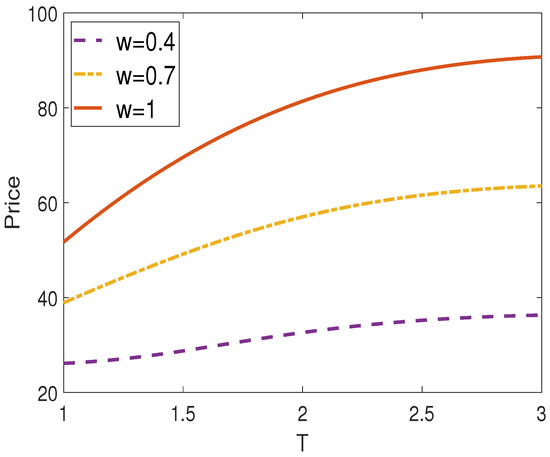
Figure 1. Vulnerable exchange option prices against maturity time T for different values w.

Figure 2 and Figure 3 illustrate the effects of the initial values of the two underlying assets. The results in Figure 2 indicate that option prices incorporating the issuer’s credit risk increase monotonically with the initial value of the first underlying asset $S_1\left(0\right)$. That is, option prices are proportional to $S_1\left(0\right)$. On the other hand, option prices are inversely proportional to the initial value of the second underlying asset $S_2\left(0\right)$. In fact, the value of $S_2\left(0\right)$ serves a similar role to the strike price of a standard European call option. Therefore, option prices decrease as $S_2\left(0\right)$ increases.

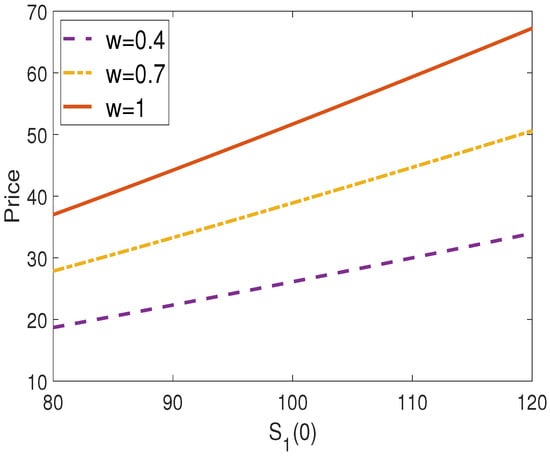
Figure 2. Vulnerable exchange option prices against initial price of underlying asset $S_1\left(t\right)$ for different values w.

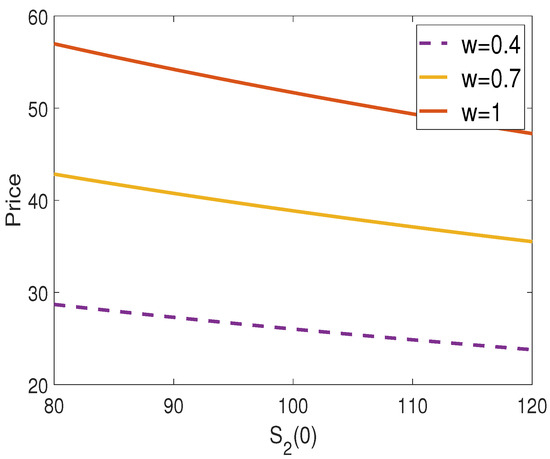
Figure 3. Vulnerable exchange option prices against initial price of underlying asset $S_2\left(t\right)$ for different values w.

From Figure 4, we observe differences in option prices when the first underlying asset has varying proportions of systematic risk ${\beta }_1$. It can be seen that option prices increase slightly with an increase in systematic risk ${\beta }_1$. Figure 5 presents the effects of different values of $\beta$ in the intensity process. The higher the value of the intensity process $\lambda \left(t\right)$, the higher the probability of a credit event. Therefore, higher values of $\beta$ result in lower option prices. However, if the recovery rate is equal to one, the value of $\beta$ has no effect.

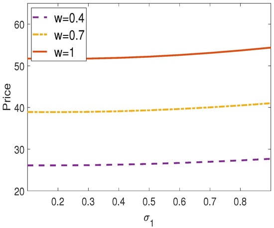
Figure 4. Vulnerable exchange option prices against ${\beta }_1$ for different values w.

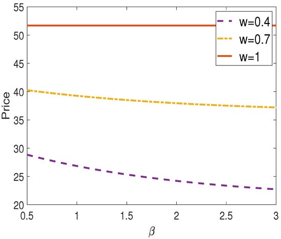
Figure 5. Vulnerable exchange option prices against $\beta$ for different values w.

5. Concluding Remarks

This paper investigates the valuation of vulnerable exchange options by incorporating a reduced-form model. In the proposed model, the processes of underlying assets are governed by a two-factor stochastic volatility model, while a mean-reverting square root process is used for the stochastic intensity process to ensure that it is positive at all times. Finally, in the proposed model, we provide the explicit solution for vulnerable exchange option pricing using the measure change technique, as well as several numerical examples to demonstrate how significant parameters impact option prices and to verify how accurate the derived formula.

References

- Merton, R.C. On the pricing of corporate debt: The risk structure of interest rates. J. Financ. 1974, 29, 449–470. [Google Scholar]
- Black, F.; Cox, J.C. Valuing corporate securities: Some effects of bond indenture provisions. J. Financ. 1976, 31, 351–367. [Google Scholar] [CrossRef]
- Jarrow, R.; Turnbull, S. Pricing options on financial securities subject to default risk. J. Financ. 1995, 50, 53–86. [Google Scholar] [CrossRef]
- Jarrow, R.A.; Yu, F. Counterparty risk and the pricing of defaultable securities. J. Financ. 2001, 56, 1765–1799. [Google Scholar] [CrossRef]
- Fard, F.A. Analytical pricing of vulnerable options under a generalized jump–diffusion model. Insur. Math. Econ. 2015, 60, 19–28. [Google Scholar] [CrossRef]
- Pasricha, P.; Goel, A. Pricing vulnerable power exchange options in an intensity based framework. J. Comput. Appl. Math. 2019, 355, 106–115. [Google Scholar] [CrossRef]
- Wang, X. Pricing European basket warrants with default risk under stochastic volatility models. Appl. Econ. Lett. 2022, 29, 253–260. [Google Scholar] [CrossRef]
- Wang, X. Analytical valuation of vulnerable European and Asian options in intensity-based models. J. Comput. Appl. Math. 2021, 393, 113412. [Google Scholar] [CrossRef]
- Wang, X. Pricing vulnerable fader options under stochastic volatility models. J. Ind. Manag. Optim. 2023, 19. [Google Scholar] [CrossRef]
- Pan, Y.; Tang, D.; Wang, X. Valuation of vulnerable European options with market liquidity risk. Probab. Eng. Informational Sci. 2024, 38, 65–81. [Google Scholar] [CrossRef]
- Wang, B.; Wang, X.; Zhao, M. Valuing Vulnerable Basket Options with Stochastic Liquidity Risk in Reduced-form Models. Comput. Econ. 2024, 1–17. [Google Scholar] [CrossRef]
- Kim, D.; Kim, G.; Yoon, J.H. Pricing of vulnerable exchange options with early counterparty credit risk. N. Am. J. Econ. Financ. 2022, 59, 101624. [Google Scholar] [CrossRef]
- Jeon, J.; Huh, J.; Kim, G. An analytical approach to the pricing of an exchange option with default risk under a stochastic volatility model. Adv. Contin. Discret. Model. 2023, 2023, 37. [Google Scholar] [CrossRef]
- Yue, S.; Ma, C.; Zhao, X.; Deng, C. Pricing power exchange options with default risk, stochastic volatility and stochastic interest rate. Commun.-Stat.-Theory Methods 2023, 52, 1431–1456. [Google Scholar] [CrossRef]
- Christoffersen, P.; Heston, S.; Jacobs, K. The shape and term structure of the index option smirk: Why multifactor stochastic volatility models work so well. Manag. Sci. 2009, 55, 1914–1932. [Google Scholar] [CrossRef]
- Cox, J.C.; Ingersoll, J.E., Jr.; Ross, S.A. A Theory of the Term Structure of Interest Rates. Econometrica 1985, 53, 385–407. [Google Scholar] [CrossRef]
- Shephard, N.G. From characteristic function to distribution function: A simple framework for the theory. Econom. Theory 1991, 7, 519–529. [Google Scholar] [CrossRef]
Disclaimer/Publisher’s Note: The statements, opinions and data contained in all publications are solely those of the individual author(s) and contributor(s) and not of MDPI and/or the editor(s). MDPI and/or the editor(s) disclaim responsibility for any injury to people or property resulting from any ideas, methods, instructions or products referred to in the content. |
© 2024 by the authors. Licensee MDPI, Basel, Switzerland. This article is an open access article distributed under the terms and conditions of the Creative Commons Attribution (CC BY) license (https://creativecommons.org/licenses/by/4.0/).