The Effect of Leachate Recycling on the Dynamics of Two Competing Bacteria with an Obligate One-Way Beneficial Relationship in a Chemostat

Abstract

In the present work, we study a simple mathematical model that describes the competition of two bacterial species with an obligate one-way beneficial relationship for a limited substrate in a bioreactor associated with leachate recirculation. The substrate is present into two forms, insoluble and soluble substrates, where the latter is consumed by the two competing bacteria, which have two general nonlinear growth rates. The reduction of the model to a 2D one facilitates the study of the nature of the equilibrium points. The dynamic system admits multiple steady states. We provide necessary and sufficient conditions on the added insoluble and soluble substrates and the dilution rate to guarantee the existence, uniqueness, and local and global stability of such steady states. It is deduced that the coexistence of both bacteria is possible, which contradicts the competitive exclusion principle. In the second step, we propose an optimal control on the leachate recirculation rate that reduces the organic matter inside the reactor. Finally, we provide some numerical examples that corroborate and reinforce the theoretical findings.

1. Introduction

A chemostat is a specific bioreactor used for the bacterial multiplication process for certain substrates in a controlled environment. In particular, the chemostat was used for the degradation of some organic matter in a liquid medium and to study the influence of such nutriment on bacterial growth. The competition between two bacteria types for a single essential resource has been considered in several theoretical studies. A classical theory result postulates that the two species cannot coexist. This result is named the competitive exclusion principle. The competitive exclusion principle was proved in several mathematical studies [1,2,3,4,5]. Several similar mathematical models were proposed and are analysed in [6,7,8,9,10,11,12,13], that aim to give an explanation of the coexistence of competing bacteria in real life through intra- and inter-specific relationships [14,15,16,17,18,19,20]. In [13,21], a viral infection was added to the competition which permits the persistence of both species.

The cooperation between different bacterial species has received great interest in recent decades since it has a major role in biodiversity [22,23]. In [24], the authors claimed that obligate intracellular bacteria can be found in all protozoa, plants, and animals, and that these specific relationships ensure the stable integration of the cell into a biological system, which is known as the endosymbiosis theory [25,26]. By using real experiments, it was deduced that in several cases, these relationships between two bacteria are obligatory and could be either in one or in both directions [27,28,29,30,31,32]. This would, of course, reflect the principle of competitive exclusion and keep the biodiversity in an ecosystem, which is also relevant from an engineering point of view. In fact, ensuring the presence of a microorganism inside an ecosystem provides several advantages. Such diversity plays a major role in several potential applications in agriculture and pollutant treatment.

In this paper, we consider an obligate one-way beneficial relationship between two species, where one species of which derives a benefit while the other suffers no harm and derives no advantage. More simply, we consider a relationship between two species in which one obtains benefits from the other without harming or benefiting it. The species that draws the benefit can be seen as a commensal, while the other can be seen as the host species [33]. Moreover, several studies have used the leachate recirculation within the waste of a waste storage center by creating favourable humidity conditions for the biodegradation of the organic matter contained in the waste [34,35]. Hence, it became possible to observe whether this technical choice allows for a reduction in the amounts of waste within this environment in the long term. Several tests were carried out in the laboratory to clarify the influence of physico-chemical factors and leachate recirculation on the characteristics of organic matter in household waste [36]. These studies demonstrate that the recirculation of leachates accelerates the production of biogas and the transfer of matter from the solid compartment to the liquid compartment [37]. Waste that has been treated with leachate recirculation shows advanced biodegradation of its organic matter compared to other waste [38]. In [39], the authors studied the problem of leachates in landfills, while [40] concerns a bioreactor in batch mode, which is the form most commonly used to model a landfill. Few mathematical works have modelled the leachate recirculation in a bioreactor [41,42,43]. In the present work, we extend the classical chemostat’s model [44] by considering a competition of two bacterial species that have an obligate one-way beneficial relationship when we recirculate the leachate inside the chemostat. The dynamics admits three steady states that we characterise in this work. Furthermore, we design an optimal control of the recirculation of leachate to optimise the organic matter inside the reactor.

The article is organised as follows: in Section 2, we present a four-dimensional dynamical system describing the competition of two bacterial species that have an obligate one-way beneficial relationship for an essential nutriment in a chemostat where the existence of the first biomass depends essentially on the presence of both the substrate and the second species, while the existence of the second species depends only on the presence of the substrate. We take into account the leachate recirculation in the reactor. In Section 3, some hypotheses on the bacterial growth rates are added, the positivity and boundedness of the solution are proved, and the definition of equilibrium points is provided. In Section 4, the four-dimensional dynamical system is reduced to planar dynamics. We discuss the existence and the stability of the equilibria of the reduced dynamics with respect to the operating parameters (substrates input concentrations and dilution rate) and the bacterial growth rates. Next, in Section 5, we discuss the global stability for the reduced dynamics and then for the main dynamics. In Section 6, we propose an optimal control strategy by minimising the organic matter inside the reactor and keeping an optimal recirculation rate for the leachate. In Section 7, we provide several numerical tests that validate the main theoretical results for both the direct and the optimal control problems. We finish the paper by providing a brief conclusion in Section 8.

2. Mathematical Model

The model proposed in this work is an extension of the classical chemostat model [44] by adding an obligate benefit relationship in one direction from the first species to the second one and by taking account of the leachate recirculation inside the reactor (see Figure 1) as it is applied in some references [39,40,41,43] with generalised growth functions. Let us denote by $S_1\left(t\right)$, $S_2\left(t\right)$, $X_1\left(t\right)$, and $X_2\left(t\right)$ the main variables of the dynamical system describing the concentrations of insoluble and soluble substrates, species 1 and species 2, present in the reactor at time t (see Figure 2).

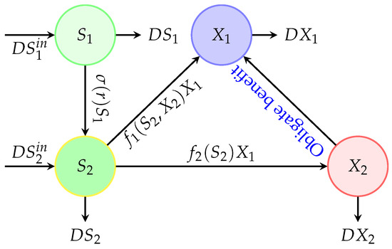
Figure 1. Interactions between two competing bacteria associated with an obligate one-way benefit and recirculation of the leachate [43].

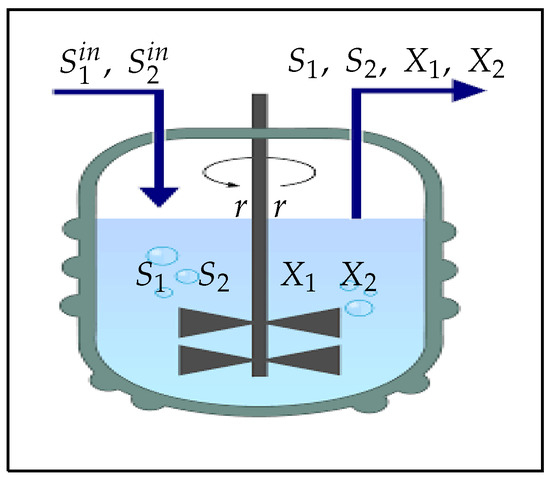
Figure 2. A classical bioreactor (Chemostat) associated with leachate recirculation [41].

Our model is given by the following four-dimensional dynamics.

$$\left\{\begin{array}{ccc}\dot{S_1}& =& D(S_1^{in}-S_1)-\sigma \left(r\right)S_1,\hfill \\ \dot{S_2}& =& D(S_2^{in}-S_2)+\sigma \left(r\right)S_1-f_1(S_2,X_2){\displaystyle \frac{X_1}{Y_1}}-f_2\left(S_2\right){\displaystyle \frac{X_2}{Y_2}},\hfill \\ {\dot{X}}_1& =& (f_1(S_2,X_2)-D)X_1,\hfill \\ {\dot{X}}_2& =& (f_2\left(S_2\right)-D)X_2,\hfill \end{array}\right.$$

(1)

where $S_1^{in}$ and $S_2^{in}$ denote the concentrations of added soluble and insoluble substrates to the reactor, respectively. $Y_1$ and $Y_2$ are the yield coefficients. D describes the rate of dilution of the reactor. The constant parameters $S_1^{in}$, $S_2^{in}$, D, $Y_1$, and $Y_2$ are positive. The growth functions $f_1:{\mathbb{R}}_{+}^2\to {\mathbb{R}}_{+}$ and $f_2:{\mathbb{R}}_{+}\to {\mathbb{R}}_{+}$ are of class $C^1$. The hydrolysis rate $\sigma :{\mathbb{R}}_{+}\to {\mathbb{R}}_{+}$ is a $C^1$ function on ${\mathbb{R}}_{+}$. More details on the variables and parameters are given in Table 1.

Table 1. Variables, functions and parameters of the dynamics (1).

Notification	Significance
$S_1$	Insoluble substrate
$S_2$	Soluble substrate
$X_1$	Species 1
$X_2$	Species 2
r	Leachate recirculation rate
$\sigma (·)$	Hydrolysis rate
$f_1(·,·)$	Growth function of bacteria 1.
$f_2(·)$	Growth function of bacteria 2.
$S_1^{in}$	Insoluble substrate input
$S_2^{in}$	Soluble substrate input
D	Dilution rate
$Y_1,Y_2$	Yield coefficients

A simple transformation of the dynamics (1) can be made through the new notations as follows: $s_1=S_1$, $s_1^{in}=S_1^{in}$, $s_2=S_2$, $s_2^{in}=S_2^{in}$, $x_1={\displaystyle \frac{X_1}{Y_1}}$, $x_2={\displaystyle \frac{X_2}{Y_2}}$, ${\mu }_1(s_2,x_2)=f_1(S_2,X_2)$, and ${\mu }_2\left(s_2\right)=f_2\left(S_2\right)$. We obtain a more simple system as follows:

$$\left\{\begin{array}{ccc}\dot{s_1}& =& D(s_1^{in}-s_1)-\sigma \left(r\right)s_1,\hfill \\ \dot{s_2}& =& D(s_2^{in}-s_2)+\sigma \left(r\right)s_1-{\mu }_1(s_2,x_2)x_1-{\mu }_2\left(s_2\right)x_2,\hfill \\ {\dot{x}}_1& =& ({\mu }_1(s_2,x_2)-D)x_1,\hfill \\ {\dot{x}}_2& =& ({\mu }_2\left(s_2\right)-D)x_2,\hfill \end{array}\right.$$

(2)

where $s_1^{in}>0$, $s_2^{in}>0$, $D>0$. The functions ${\mu }_1:{\mathbb{R}}_{+}^2\to {\mathbb{R}}_{+}$, ${\mu }_2:{\mathbb{R}}_{+}\to {\mathbb{R}}_{+}$, and $\sigma :{\mathbb{R}}_{+}\to {\mathbb{R}}_{+}$ are of class $C^1$ satisfying:

A1.

${\mu }_2\left(0\right)=0$, ${\mu }_2^{\prime }\left(s_2\right)>0$, $\forall s_2\in {\mathbb{R}}_{+}$.

A2.

${\mu }_1(s_2,0)={\mu }_1(0,x_2)=0$, $\forall s_2,x_2\in {\mathbb{R}}_{+}$.

A3.

${\displaystyle \frac{\partial {\mu }_1}{\partial s_2}}(s_2,x_2)>0$, $\forall (s_2,x_2)\in {\mathbb{R}}_{+}^2$.

A4.

${\displaystyle \frac{\partial {\mu }_2}{\partial x_2}}(s_2,x_2)>0$, $\forall (s_2,x_2)\in {\mathbb{R}}_{+}^2$.

A5.

$\sigma (·)$ is increasing such that $\sigma \left(0\right)=0$.

Assumption A1 expresses that no growth can be possible without the presence of the soluble substrate for bacteria 2, and that bacteria 2 growth increases with the soluble substrate concentration. Assumption A2 expresses that no growth can be possible without both soluble substrate and species 2 for species 1. Assumptions A3 and A4 express that species 1 growth increases with both soluble substrate and species 2. $X_2$ (species 2) favors the growth of $X_1$ (species 1), while $X_1$ (species 1) has no direct action on $X_2$ (species 2) apart from competition for substrate. Assumption A5 confirms that no production of soluble substrate can take place without leachate recirculation associated with the presence of the insoluble substrate that will be converted into a soluble one.

Remark 1. 

The function of Holling type II known also as Monod functions [45,46] can express growth rates that satisfy all previous assumptions: A1 to A4.

$${\mu }_1(s_2,x_2)={\displaystyle \frac{{\overline{\mu }}_1{s}_2{x}_2}{(1+p_1{s}_2)(1+q{x}_2)}}\mathit{and}{\mu }_2\left(s_2\right)={\displaystyle \frac{{\overline{\mu }}_2{s}_2}{(1+p_2{s}_2)}},$$

where the constants ${\overline{\mu }}_1$, ${\overline{\mu }}_2$, $p_1$, $p_2$, and q are positive.

3. Basic Properties

Lemma 1. 

If the function $\sigma :{\mathbb{R}}_{+}\to {\mathbb{R}}_{+}$ satisfies Assumption A5, then there exists a unique value $s_1^{\ast }\in (0,s_1^{in})$ satisfying

$$\sigma \left(r\right)s_1^{\ast }=D(s_1^{in}-s_1^{\ast }),$$

(3)

where $s_1^{\ast }={\displaystyle \frac{D{s}_1^{in}}{D+\sigma \left(r\right)}}$.

Proof. 

Consider the function $\tau \left(s_1\right)=D(s_1^{in}-s_1)-\sigma \left(r\right)s_1$; thus, ${\tau }^{\prime }\left(s_1\right)=-D-\sigma \left(r\right)<0$, $\tau \left(0\right)=D{s}_1^{in}>0$, and $\tau \left(s_1^{in}\right)=-\sigma \left(r\right)s_1^{in}<0$. Then, there exists a unique value $s_1^{\ast }\in (0,s_1^{in})$ that satisfies (3).    □

Consider the following assumption on the species 2 growth rate ${\mu }_2$.

A6.

${\mu }_2(s_1^{in}+s_2^{in}-s_1^{\ast })>D$.

Lemma 2. 

If ${\mu }_2:{\mathbb{R}}_{+}\to {\mathbb{R}}_{+}$ satisfies assumptions A1 and A6, then there exists a unique value $s_2^{\ast }\in (0,s_1^{in}+s_2^{in}-s_1^{\ast })$ that satisfies

$${\mu }_2\left(s_2^{\ast }\right)=D.$$

(4)

Proof. 

It is evident because ${\mu }_2$ is an increasing function that satisfies ${\mu }_2\left(0\right)=0$, ${\mu }_2(s_1^{in}+s_2^{in}-s_1^{\ast })>D$.    □

Consider the following assumption on the species 1 growth rate ${\mu }_1$.

A7.

${\mu }_1(s_2^{\ast },s_1^{in}+s_2^{in}-s_1^{\ast }-s_2^{\ast })>D$.

Lemma 3. 

Under assumptions A2, A4, and A7, then there exists a unique value $x_2^{\ast }$ such that $x_2^{\ast }\in \left(0,s_1^{in}+s_2^{in}-s_1^{\ast }-s_2^{\ast }\right)$ satisfying

$${\mu }_1(s_2^{\ast },x_2^{\ast })=D.$$

(5)

Proof. 

It is evident because ${\mu }_1(s_2^{\ast },s_1^{in}+s_2^{in}-s_1^{\ast }-s_2^{\ast })>D$, ${\mu }_1(s_2^{\ast },0)=0$ and $x_2\to {\mu }_1(s_2^{\ast },x_2)$ is an increasing function.    □

The solution of the dynamics (2) is defined on the non-negative cone [44] and satisfies the following Proposition.

Proposition 1. 

1. 

All solutions of the dynamics (2) are non-negative and bounded.

2. 

$\mathsf{\Omega }=\left\{(s_1,s_2,x_1,x_2)\in {\mathbb{R}}_{+}^4|s_1+s_2+x_1+x_2=s_1^{in}+s_2^{in}\right\}$ is a positively invariant set attracting all solutions of the dynamics (2).

Proof. 

• ${\mathbb{R}}_{+}^4$ is invariant since we have $s_1\left(t\right)=0\Rightarrow {\dot{s}}_1\left(t\right)=D{s}_1^{in}>0$, $s_2\left(t\right)=0\Rightarrow {\dot{s}}_2\left(t\right)=D{s}_2^{in}+\sigma \left(r\right)s_1>0$, $x_i\left(t\right)=0\Rightarrow {\dot{x}}_i\left(t\right)=0$ for $i=1,2$.
  Consider the variable $V\left(t\right)=s_1\left(t\right)+s_2\left(t\right)+x_1\left(t\right)+x_2\left(t\right)-s_1^{in}-s_2^{in}$. The sum of the four equations of system (2) gives us

  $$\dot{V}\left(t\right)=-DV\left(t\right).$$

  (6)
  Thus, $s_1\left(t\right)+s_2\left(t\right)+x_1\left(t\right)+x_2\left(t\right)=s_1^{in}+s_2^{in}+V\left(0\right)e^{-Dt}$ with $V\left(0\right)=s_1\left(0\right)+s_2\left(0\right)+x_1\left(0\right)+x_2\left(0\right)-s_1^{in}-s_2^{in}$. As all components of $V\left(t\right)$ are non-negative, thus, we obtain the boundedness of the solution.
• It is deduced from Equation (6).    □

Lemma 4. 

Let $(s_1,s_2,x_1,x_2)$ be a solution of the system (2). Consider

$${\rho }_1=s_1-s_1^{\ast } and {\rho }_2=s_1^{in}+s_2^{in}-s_1-s_2-x_1-x_2=s_1^{in}+s_2^{in}-s_1^{\ast }-{\rho }_1-s_2-x_1-x_2.$$

(7)

Then,

$$\begin{array}{lll}{\dot{\rho }}_1& =& -[D+\sigma \left(r\right)]{\rho }_1,\hfill \end{array}$$

(8)

$$\begin{array}{lll}{\dot{\rho }}_2& =& -D{\rho }_2,\hfill \end{array}$$

(9)

and

$$\left\{\begin{array}{ccc}{\dot{x}}_1& =& ({\mu }_1(s_1^{in}+s_2^{in}-s_1^{\ast }-{\rho }_1-{\rho }_2-x_1-x_2,x_2)-D)x_1,\hfill \\ {\dot{x}}_2& =& ({\mu }_2(s_1^{in}+s_2^{in}-s_1^{\ast }-{\rho }_1-{\rho }_2-x_1-x_2)-D)x_2.\hfill \end{array}\right.$$

(10)

Let us now study the nature of the equilibrium points of the system (2).

Theorem 1. 

Assume that the functions of system (2) verify Assumptions A1 to A7. Then, the system (2) has three equilibrium points given by

$$\begin{array}{l}\begin{array}{c}{E}^0=(s_1^{\ast },s_1^{in}+s_2^{in}-s_1^{\ast },0,0),E^2=(s_1^{\ast },s_2^{\ast },0,s_1^{in}+s_2^{in}-s_1^{\ast }-s_2^{\ast }) and E^{\ast }=(s_1^{\ast },s_2^{\ast },x_1^{\ast },x_2^{\ast }),\hfill \end{array}\end{array}$$

where $s_1^{\ast }$ is defined by Lemma 1, $s_2^{\ast }$ is defined by Lemma 2, $x_2^{\ast }$ is defined by Lemma 3, and $x_1^{\ast }=s_1^{in}+s_2^{in}-s_1^{\ast }-s_2^{\ast }-x_2^{\ast }$.

Proof. 

Assume that the functions of system (2) verify Assumptions A1 to A7. Let $E^e=(s_1^e,s_2^e,p^e,x_1^e,x_2^e)$ be a non-negative equilibrium point of system (2); then, we obtain

$$\left\{\begin{array}{ccc}\sigma \left(r\right)s_1^e\hfill & =\hfill & D(s_1^{in}-s_1^e),\hfill \\ {\mu }_1(s_2^e,x_2^e)x_1^e\hfill & =\hfill & D{x}_1^e,\hfill \\ {\mu }_2\left(s_2^e\right)x_2^e\hfill & =\hfill & D{x}_2^e,\hfill \\ s_1^e+s_2^e+x_1^e+x_2^e\hfill & =\hfill & s_1^{in}+s_2^{in}.\hfill \end{array}\right.$$

(11)

If $x_1^e=0$, then $s_1^e=s_1^{\ast }$, and either $x_2^e=0$ and then $E^e=E^0$ or $x_2^e\ne 0$ and then $s_2^e=s_2^{\ast }$ and $x_2^e=s_1^{in}+s_2^{in}-s_2^{\ast }$; therefore, we obtain $E^e=E^2$. The case $x_1\ne 0$ and $x_2=0$ is impossible, since ${\mu }_1(s_2^e,0)=0\ne D$. Still, there is the case when $x_1\ne 0$ and $x_2\ne 0$. Then, we obtain $\sigma \left(r\right)s_1^e=D(s_1^{in}-s_1^e)$, ${\mu }_1(s_2^e,x_2^e)={\mu }_2\left(s_2^e\right)=D$, and $s_1^e+s_2^e+x_1^e+x_2^e=s_1^{in}+s_2^{in}$. From Lemmas 1–3, we deduce that $s_1^e=s_1^{\ast }$, $s_2^e=s_2^{\ast }$ and $x_2^e=x_2^{\ast }$ and thus $x_1^{\ast }=s_1^{in}+s_2^{in}-s_1^{\ast }-s_2^{\ast }-x_2^{\ast }$. Therefore, we deduce the uniqueness of the positive equilibrium point, $E^e=E^{\ast }$.    □

4. Reduced System

In order to study the stability of model (2), we can restrict system (2) to the invariant attractor set $\Omega$ to obtain the following planar system.

$$\left\{\begin{array}{ccc}{\dot{x}}_1& =& {\psi }_1(x_1,x_2),\hfill \\ {\dot{x}}_2& =& {\psi }_2(x_1,x_2),\hfill \end{array}\right.$$

(12)

with

$$\left(\begin{array}{c}{\psi }_1(x_1,x_2)\\ {\psi }_2(x_1,x_2)\end{array}\right)=\left(\begin{array}{c}({\mu }_1(s_1^{in}+s_2^{in}-s_1^{\ast }-x_1-x_2,x_2)-D)x_1\\ ({\mu }_2(s_1^{in}+s_2^{in}-s_1^{\ast }-x_1-x_2)-D)x_2\end{array}\right),$$

and

$$\mathcal{S}=\left\{(x_1,x_2)\in {\left({\mathbb{R}}_{+}^{\ast }\right)}^2:0<x_1+x_2<s_1^{in}+s_2^{in}-s_1^{\ast }\right\},$$

(13)

as state space. Observe that the dynamics (2) and (10) are equivalent and that the dynamics (12) is deduced when considering the dynamics (10) such that ${\rho }_1=0$ and ${\rho }_2=0$.

According to Theorem 1, the planar dynamics (12) admits three equilibrium points given by $F^0=(0,0)$, $F^2=(0,s_1^{in}+s_2^{in}-s_1^{\ast }-s_2^{\ast })$ and $F^{\ast }=(x_1^{\ast },x_2^{\ast })$.

Lemma 5. 

Assume that Assumptions A1 to A7 are satisfied. Therefore, $F^0$ and $F^2$ are saddle points and $F^{\ast }$ is a locally exponentially stable equilibrium point for system (12).

Proof. 

The Jacobian matrix is given by

$$J(x_1,x_2)=\left[\begin{array}{ll}{\mu }_1-D-{\displaystyle \frac{\partial {\mu }_1}{\partial s_2}}{x}_1& -{\displaystyle \frac{\partial {\mu }_1}{\partial s_2}}{x}_1+{\displaystyle \frac{\partial {\mu }_1}{\partial x_2}}{x}_1\\ \hfill -{\mu }_2^{\prime }{x}_2\hfill & {\mu }_2-D-{\mu }_2^{\prime }{x}_2\end{array}\right],$$

such that ${\mu }_1$ is expressed at $(s_1^{in}+s_2^{in}-s_1^{\ast }-x_1-x_2,x_2)$ and ${\mu }_2$ is expressed at $(s_1^{in}+s_2^{in}-s_1^{\ast }-x_1-x_2)$. Let us study the matrices $J\left(F^0\right)$, $J\left(F^2\right)$ and $J\left(F^{\ast }\right)$. Since

$$J\left(F^0\right)=\left[\begin{array}{cc}-D& \hfill 0\hfill \\ 0& {\mu }_2(s_1^{in}+s_2^{in}-s_1^{\ast })-D\end{array}\right],$$

then the eigenvalues are $X_1=-D<0$ and $X_2={\mu }_2(s_1^{in}+s_2^{in}-s_1^{\ast })-D>0$ according to Assumption A6. Consequently, $F^0$ is a saddle point of (12). The matrix at $J\left(F^2\right)$ is given by

$$J\left(F^2\right)=\left[\begin{array}{ll}{\mu }_1(s_2^{\ast },s_2^{in}+s_1^{in}-s_1^{\ast }-s_2^{\ast })-D& \hfill 0\hfill \\ -{\mu }_2^{\prime }\left(s_2^{\ast }\right)(s_2^{in}+s_1^{in}-s_1^{\ast }-s_2^{\ast })& -{\mu }_2^{\prime }\left(s_2^{\ast }\right)(s_2^{in}+s_1^{in}-s_1^{\ast }-s_2^{\ast })\end{array}\right].$$

Their eigenvalues are $X_1={\mu }_1(s_2^{\ast },s_1^{in}+s_2^{in}-s_1^{\ast }-s_2^{\ast })-D>0$ by Assumption A7 and $X_2=-{\mu }_2^{\prime }\left(s_2^{\ast }\right)(s_1^{in}+s_2^{in}-s_1^{\ast }-s_2^{\ast })<0$. Consequently, $F^2$ is a saddle point of (12).

The matrix at $J\left(F^{\ast }\right)$ is given by

$$J\left(F^{\ast }\right)=\left[\begin{array}{ll}-{\displaystyle \frac{\partial {\mu }_1(s_2^{\ast },x_2^{\ast })}{\partial s_2}}{x}_1^{\ast }& -{\displaystyle \frac{\partial {\mu }_1(s_2^{\ast },x_2^{\ast })}{\partial s_2}}{x}_1^{\ast }+{\displaystyle \frac{\partial {\mu }_1(s_2^{\ast },x_2^{\ast })}{\partial x_2}}{x}_1^{\ast }\\ \hfill -{\mu }_2^{\prime }\left(s_2^{\ast }\right)x_2^{\ast }\hfill & \hfill -{\mu }_2^{\prime }\left(s_2^{\ast }\right)x_2^{\ast }\hfill \end{array}\right].$$

(14)

Note that

$$\mathrm{t}\mathrm{r}\left(J\left(F^{\ast }\right)\right)=-{\displaystyle \frac{\partial {\mu }_1(s_2^{\ast },x_2^{\ast })}{\partial s_2}}{x}_1^{\ast }-{\mu }_2^{\prime }\left(s_2^{\ast }\right)x_2^{\ast }<0,$$

and

$$\mathrm{d}\mathrm{e}\mathrm{t}\left(J\left(F^{\ast }\right)\right)={\mu }_2^{\prime }\left(s_2^{\ast }\right)x_2^{\ast }{\displaystyle \frac{\partial {\mu }_1(s_2^{\ast },x_2^{\ast })}{\partial x_2}}{x}_1^{\ast }>0.$$

Thus, $J\left(F^{\ast }\right)$ has two eigenvalues with negative real parts, and then the equilibrium point $F^{\ast }$ is locally exponentially stable.    □

Theorem 2. 

Assume that Assumptions A1 to A7 are verified. Therefore, $E^0$ and $E^2$ are saddle points; however, $E^{\ast }$ is a locally exponentially stable equilibrium point.

Proof. 

It is evident that the equilibrium points $E^0$, $E^2$ and $E^{\ast }$ have the same nature as the equilibrium points $F^0$, $F^2$ and $F^{\ast }$, respectively.    □

5. Global Analysis

We start by studying the global stability of the reduced system (12). Then, we deduce on the global stability of (2).

5.1. Global Stability of (12)

We start by proving that $\mathcal{S}$ and $\overline{\mathcal{S}}$ are positively invariant sets and that system (12) has no possible periodic orbits inside $\overline{\mathcal{S}}$.

Lemma 6. 

Assume that Assumptions A1–A7 hold. The sets $\mathcal{S}$ and $\overline{\mathcal{S}}$ are positively invariant sets. Furthermore, the model (12) admits no periodic solution inside $\overline{\mathcal{S}}$.

Proof. 

We can verify that $\mathcal{S}$ and $\overline{\mathcal{S}}$ are positively invariant, since we have

$${\dot{x}}_1+{\dot{x}}_2={\mu }_1(s_1^{in}+s_2^{in}-s_1^{\ast }-(x_1+x_2),x_2)x_1+{\mu }_2(s_1^{in}+s_2^{in}-s_1^{\ast }-(x_1+x_2))x_2-D(x_1+x_2).$$

Now, consider a solution of (12) inside $\mathcal{S}$, and we aim to exclude the possibility of a periodic solution inside $\mathcal{S}$.

Notice that axis $x_1=0$ and $x_2=0$ are invariant. By using the change of variables ${\zeta }_1=ln\left(x_1\right)$ and ${\zeta }_2=ln\left(x_2\right)$ for $x_1,x_2>0$. Thus, we obtain the new dynamics given hereafter:

$$\left\{\begin{array}{c}{\displaystyle {\dot{\zeta }}_1=g_1({\zeta }_1,{\zeta }_2):={\mu }_1(s_1^{in}+s_2^{in}-s_1^{\ast }-e^{{\zeta }_1}-e^{{\zeta }_2},e^{{\zeta }_2})-D,}\hfill \\ {\displaystyle {\dot{\zeta }}_2=g_2({\zeta }_1,{\zeta }_2):={\mu }_2(s_1^{in}+s_2^{in}-s_1^{\ast }-e^{{\zeta }_1}-e^{{\zeta }_2})-D.}\hfill \end{array}\right.$$

(15)

Note that for $e^{{\zeta }_1}+e^{{\zeta }_2}<s_1^{in}+s_2^{in}-s_1^{\ast }$, we have

$$\begin{array}{ccc}{\displaystyle \frac{\partial g_1}{\partial {\zeta }_1}}+{\displaystyle \frac{\partial g_2}{\partial {\zeta }_2}}\hfill & =\hfill & -{\displaystyle \frac{\partial {\mu }_1}{\partial s_2}}(s_1^{in}+s_2^{in}-s_1^{\ast }-e^{{\zeta }_1}-e^{{\zeta }_2},e^{{\zeta }_2})e^{{\zeta }_1}\hfill \\ \hfill & \hfill & -{\mu }_2^{\prime }(s_1^{in}+s_2^{in}-s_1^{\ast }-e^{{\zeta }_1}-e^{{\zeta }_2})e^{{\zeta }_2}<0.\hfill \end{array}$$

(16)

We consider the criterion of Dulac (see [47], Chapter 6) when applied to (15) for trajectories belonging to the simply connected region

$${\displaystyle \mathcal{D}=\left\{({\zeta }_1,{\zeta }_2)\in {\mathbb{R}}^2:e^{{\zeta }_1}+e^{{\zeta }_2}<s_1^{in}+s_2^{in}-s_1^{\ast }\right\}.}$$

Since ${\displaystyle \frac{\partial g_1}{\partial {\zeta }_1}}+{\displaystyle \frac{\partial g_2}{\partial {\zeta }_2}}$ does not change signs in $\mathcal{D}$, this criterion ensures that the system (15) has no periodic trajectory in $\mathcal{D}$. Then, the dynamics (12) has no periodic orbit in $\mathcal{S}$. It cannot have polycycles because there is only one equilibrium point in $\mathcal{S}$. Next, let us proceed by contradiction to prove that the system (12) has no periodic orbit inside $\overline{\mathcal{S}}$. Suppose that there exists in $\overline{\mathcal{S}}$ a periodic solution of (12) that we denote $(x_1\left(t\right),x_2\left(t\right))$. We deduce easily from the fact that $\mathcal{S}$ is positively invariant that necessarily either $x_1\left(t\right)=0$ for all $t\ge 0$ or $x_2\left(t\right)=0$ for all $t\ge 0$. If $x_1\left(t\right)=0$ for all $t\ge 0$; then, necessarily, for all $t\ge 0$, ${\dot{x}}_2\left(t\right)=[{\mu }_2(s_1^{in}+s_2^{in}-s_1^{\ast }-x_2\left(t\right))-D]x_2\left(t\right)$. Thanks to Assumptions A1 to A7, we deduce that necessarily, $x_2\left(t\right)$ converges either to 0 or to $s_1^{in}+s_2^{in}-s_1^{\ast }-s_2^{\ast }$ when the time tends to the infinity. If $x_2\left(t\right)=0$ for all $t\ge 0$, then necessarily, for all $t\ge 0$, ${\dot{x}}_1\left(t\right)=-D{x}_1\left(t\right)$ and $x_1\left(t\right)$ converges to zero when the time tends to the infinity. This concludes the proof.    □

We are ready to establish a crucial result for planar system (12).

Theorem 3. 

Suppose that Assumptions A1 to A7 are satisfied and consider system (12). Then, the point $F^{\ast }$ is a globally asymptotically stable equilibrium point of (12) on $\mathcal{S}$.

Proof. 

Consider a solution $(x_1\left(t\right),x_2\left(t\right))$ of (12) belonging to $\mathcal{S}$. The system (12) has no unbounded trajectory in $\mathcal{S}$ because $\overline{\mathcal{S}}$ is a positively invariant compact set. Therefore, $(x_1\left(t\right),x_2\left(t\right))$ is a bounded trajectory. Consequently, it admits a compact $\omega$-limit set, that we denote $\omega$, which is included in $\overline{\mathcal{S}}$. According to the Poincaré–Bendixon Theorem [47], $\omega$ either contains an equilibrium point or (12) admits a periodic solution in $\overline{\mathcal{S}}$. Since Lemma 6 ensures that there exist no periodic solutions of (12) in $\overline{\mathcal{S}}$, necessarily $\omega$ contains an equilibrium point of (12). The system (12) admits three equilibrium points $F^0$, $F^2$ and $F^{\ast }$. $F^0$ and $F_2$ are saddle points, and only $F^{\ast }$ is a stable node. If $F^{\ast }\in \omega$, then $F^{\ast }=\omega$ because $F^{\ast }$ is locally exponentially stable (see Lemma 5). Next, let us prove that $F^{\ast }\in \omega$ by proceeding by contradiction.

Let $x_1\left(0\right)>0,x_2\left(0\right)>0$. $\omega$ is an invariant compact set and $\omega \subset \overline{\mathcal{S}}$. Assume that $\omega$ contains a point M on the $x_1{x}_2$ axis:

• M cannot be $F_0$, because $F_0$ is an unstable node and cannot be a part of the $\omega$-limit set of $(x_1\left(0\right),x_2\left(0\right))$;
• If $M\in ]0,s_1^{in}+s_2^{in}-s_1^{\ast }-s_2^{\ast }[\times \left\{0\right\}$. $\omega$ contains $\gamma \left(M\right)=]0,s_1^{in}+s_2^{in}-s_1^{\ast }-s_2^{\ast }[\times \left\{0\right\}$. Since $\omega$ is compact, then it contains the adherence $[0,s_1^{in}+s_2^{in}-s_1^{\ast }-s_2^{\ast }]\times \left\{0\right\}$; thus, $\omega$ contains $F^0$, which is not possible;
• If $M\in \left\{0\right\}\times ]s_1^{in}+s_2^{in}-s_1^{\ast }-s_2^{\ast },s_1^{in}+s_2^{in}-s_1^{\ast }]$. As $\omega$ is invariant, then $\gamma \left(M\right)\subset \omega$, which is not possible since $\omega$ is bounded and $\gamma \left(M\right)=\left\{0\right\}\times ]s_1^{in}+s_2^{in}-s_1^{\ast }-s_2^{\ast },+\infty [$;
• If $M\in \left\{0\right\}\times ]0,s_1^{in}+s_2^{in}-s_1^{\ast }-s_2^{\ast }[$. $\omega$ contains $\gamma \left(M\right)=\left\{0\right\}\times ]0,s_1^{in}+s_2^{in}-s_1^{\ast }-s_2^{\ast }[$. Since $\omega$ is compact, then it contains the adherence $\left\{0\right\}\times [0,s_1^{in}+s_2^{in}-s_1^{\ast }-s_2^{\ast }]$ and then $\omega$ contains $F^0$, which is not possible;
• If $M=F^2$, then $\omega$ is not reduced to $F^2$. Using the theorem of Butler–McGehee, we deduce that $\omega$ contains a point P of $\left\{0\right\}\times (0,+\infty )$ other that $F_2$, which is not possible.

Thus, the $\omega$-limit set cannot contain any point from the $x_1{x}_2$ axis. This allows us to conclude that all the trajectories of the dynamics (12) in $\mathcal{S}$ converge asymptotically to $F^{\ast }$.    □

5.2. Global Analysis of the Main Dynamics (2)

In this section, we aim to prove the main results of this paper.

Theorem 4. 

Suppose that the dynamics (2) satisfies Assumptions A1 to A7. Therefore, the steady state $E^{\ast }$ is globally asymptotically stable.

Proof. 

Theorem 4 will be proved by using an approach applied in [16] since the dynamics of the system (12) admits only stable and unstable steady states, and there are neither periodic trajectories nor cyclic chains. By using the results of Theme [48], we deduce the asymptotic behaviors of the trajectories of the main dynamics (2) from the asymptotic behaviors of the trajectories of the reduced dynamics (12). Let $(s_1\left(t\right),s_2\left(t\right),x_1\left(t\right),x_2\left(t\right))$ be a solution of (2). Therefore, $(x_1\left(t\right),x_2\left(t\right))$ is a trajectory of the following non-autonomous system:

$$\begin{array}{l}\left\{\begin{array}{ccc}{\dot{x}}_1\hfill & =\hfill & ({\mu }_1(s_1^{in}+s_2^{in}-s_1^{\ast }-{\rho }_1-{\rho }_2-x_1-x_2,x_2)-D)x_1,\hfill \\ {\dot{x}}_2\hfill & =\hfill & ({\mu }_2(s_1^{in}+s_2^{in}-s_1^{\ast }-{\rho }_1-{\rho }_2-x_1-x_2)-D)x_2,\hfill \end{array}\right.\end{array}$$

(17)

where ${\rho }_1$ and ${\rho }_2$ are solutions of Equations (8) and (9), which converge asymptotically to zero. This dynamics (17) is a non-autonomous dynamics which converges to the autonomous dynamics (12). Note that the reduced system (12) admits only locally stable and unstable steady states, and there are no periodic trajectories nor cyclic chains. Therefore, by using the theory of Thieme [48], we conclude that the asymptotic behaviours of the trajectories of the main dynamics (17) from the asymptotic behaviours of the trajectories of the reduced dynamics (12). This allows us to conclude.    □

Remark 2. 

An alternative way to prove Theorem 4 is by considering the new coordinates

$${\rho }_1=s_1-s_1^{\ast }, and {\rho }_2=s_1^{in}+s_2^{in}-s_1-s_2-x_1-x_2=s_1^{in}+s_2^{in}-s_1^{\ast }-{\rho }_1-s_2-x_1-x_2,$$

which leads us to consider the system

$$\left\{\begin{array}{ccc}\dot{\omega }& =& A\omega ,\hfill \\ {\dot{x}}_1& =& ({\mu }_1(s_1^{in}+s_2^{in}-s_1^{\ast }-{\rho }_1-{\rho }_2-x_1-x_2,x_2)-D)x_1,\hfill \\ {\dot{x}}_2& =& ({\mu }_2(s_1^{in}+s_2^{in}-s_1^{\ast }-{\rho }_1-{\rho }_2-x_1-x_2)-D)x_2,\hfill \end{array}\right.$$

(18)

with ${\displaystyle \omega ={({\rho }_1,{\rho }_2)}^{\top }}$, $A=\left(\begin{array}{cc}-(D+\sigma (r\left)\right)& 0\\ 0& -D\end{array}\right)$. Therefore, since the dynamics (18) satisfies the assumptions given in [44] (Appendix F), we can conclude on the global asymptotic stability of the equilibrium point $E^{\ast }$.

For the rest of the paper, we assume that $\sigma \left(r\right)=\overline{\sigma }r$ with $\overline{\sigma }>0$ is a constant.

6. Optimal Control on Leachate Recirculation

Assume that the leachate is added to the reactor continuously with a rate r which is different to the dilution rate, D. The main goal of the optimal strategy is to reduce the organic matter $(s_1\left(t\right),s_2\left(t\right))$ inside the chemostat through an optimal rate for leachate recirculation. Therefore, we will assume that the rate $r\left(t\right)$ (recirculation costs) is variable on the time interval $[0,T]$ where $T>0$ is a constant. Assume that ${\mu }_1$ and ${\mu }_2$ are globally Lipschitz having Lipschitz constants $L_1$ and $L_2$, respectively, with  upper bounds ${\displaystyle {\mu }_1^{max}=\underset{s_2,x_2>0}{sup}{\mu }_1(s_2,x_2)}$ and ${\displaystyle {\mu }_2^{max}=\underset{s_2>0}{sup}{\mu }_2\left(s_2\right)}$, respectively. Therefore, the goal is to find the optimal control function $r=r\left(t\right)$ in the admissible set

$$P_{ad}=\{r\left(t\right):0\le r^{\min }\le r\left(t\right)\le r^{\max },0\le t\le T,r\left(t\right)\mathrm{is}\mathrm{Lebesgue}\mathrm{measurable}\}.$$

minimising the functional given hereafter:

$$J\left(r\right)={\displaystyle \frac{{\kappa }_1}{2}}{\int }_0^T{s}_1^2\left(t\right)dt+{\displaystyle \frac{{\kappa }_2}{2}}{\int }_0^T{s}_2^2\left(t\right)dt+{\displaystyle \frac{{\kappa }_3}{2}}{\int }_0^T{r}^2\left(t\right)dt.$$

For appropriate values of the constants ${\kappa }_1>0,{\kappa }_2>0$ and ${\kappa }_3>0$, we aim to minimise the quantity of the organic matter in its two forms and keeping minimal the control cost. By using the theory in [49], one can easily prove that both the optimal control and the state exist. For $\phi ={\left(s_1,s_2,x_1,x_2\right)}^t$, the model (2) can be written as follows

$$\begin{array}{l}\begin{array}{c}{\displaystyle \dot{\phi }=B\phi +H_1\left(\phi \right)=H_2\left(\phi \right)}\hfill \end{array}\end{array}$$

(19)

with $B=\left(\begin{array}{cccc}-D& 0& 0& 0\\ 0& -D& 0& 0\\ 0& 0& -D& 0\\ 0& 0& 0& -D\end{array}\right)$ and

$$H_1\left(\phi \right)=\left(\begin{array}{c}D{s}_1^{in}-\overline{\sigma }r{s}_1\\ D{s}_2^{in}+\overline{\sigma }r{s}_1-{\mu }_1(s_2,x_2)x_1-{\mu }_2\left(s_2\right)x_2\\ {\mu }_1(s_2,x_2)x_1\\ {\mu }_2\left(s_2\right)x_2\end{array}\right).$$

Theorem 5. 

The continuous function $H_2$ is uniformly Lipschitz.

Proof. 

One can see that the continuous function $H_1$ is uniformly Lipschitz once it satisfies

$$\begin{array}{c}\hfill \begin{array}{ccc}\hfill \parallel H_1\left({\phi }^{\prime }\right)-H_1\left(\phi \right){\parallel }_1& =\hfill & {\displaystyle |\overline{\sigma }r{s}_1^{\prime }-\overline{\sigma }r{s}_1|+|{\mu }_1(s_2^{\prime },x_2^{\prime })x_1^{\prime }-{\mu }_1(s_2,x_2)x_1|}\hfill \\ & & +|{\mu }_2\left(s_2^{\prime }\right)x_2^{\prime }-{\mu }_2\left(s_2\right)x_2|+|\overline{\sigma }r{s}_1^{\prime }-\overline{\sigma }r{s}_1\hfill \\ & & -({\mu }_1(s_2^{\prime },x_2^{\prime })x_1^{\prime }-{\mu }_1(s_2,x_2)x_1)-({\mu }_2\left(s_2^{\prime }\right)x_2^{\prime }-{\mu }_2\left(s_2\right)x_2)|\hfill \\ & \le \hfill & 2\overline{\sigma }r|s_1^{\prime }-s_1|+2|{\mu }_1(s_2^{\prime },x_2^{\prime })x_1^{\prime }-{\mu }_1(s_2,x_2)x_1|\hfill \\ & & +2|{\mu }_2\left(s_2^{\prime }\right)x_2^{\prime }-{\mu }_2\left(s_2\right)x_2|\hfill \\ & \le \hfill & {\displaystyle 2\overline{\sigma }{r}^{max}|s_1^{\prime }-s_1|+2{\mu }_1^{max}|x_1^{\prime }-x_1|}\hfill \\ & & +2(s_1^{in}+s_2^{in})L_1|(s_2^{\prime },x_2^{\prime })-(s_2,x_2)|\hfill \\ & & +2{\mu }_2^{max}|x_2^{\prime }-x_2|+2(s_1^{in}+s_2^{in})L_2|x_2^{\prime }-x_2|\hfill \\ & \le \hfill & {\displaystyle L\parallel {\phi }_1-{\phi }_2{\parallel }_1,}\hfill \end{array}\end{array}$$

where $L=\max (2\overline{\sigma }{r}^{max},2{\mu }_1^{max},2(s_1^{in}+s_2^{in})L_1,2{\mu }_2^{max},2(s_1^{in}+s_2^{in})L_2)$. The matrix B satisfies

$${\displaystyle \parallel B{\phi }_1-B{\phi }_2{\parallel }_1\le D\parallel {\phi }_1-{\phi }_2{\parallel }_1,}$$

thus,

$${\displaystyle \parallel H_2\left({\phi }_1\right)-H_2\left({\phi }_2\right){\parallel }_1\le \delta \parallel {\phi }_1-{\phi }_2{\parallel }_1,}$$

with $\delta =\max (L,D)$ and thus the continuous function, $H_2$ is uniformly Lipschitz.    □

Thus, the dynamics (19) has a unique solution. By using Pontryagin’s maximum principle [49,50,51], the control problem can be studied using the Hamiltonian function as follows:

$$\begin{array}{ccc}H\hfill & =\hfill & {\displaystyle \frac{{\kappa }_1}{2}}{s}_1^2+{\displaystyle \frac{{\kappa }_2}{2}}{s}_2^2+{\displaystyle \frac{{\kappa }_3}{2}}{r}^2+{\lambda }_1{\dot{s}}_1+{\lambda }_2{\dot{s}}_2+{\lambda }_3{\dot{x}}_1+{\lambda }_4{\dot{x}}_2\hfill \\ & =& {\displaystyle \frac{{\kappa }_1}{2}}{s}_1^2+{\displaystyle \frac{{\kappa }_2}{2}}{s}_2^2+{\displaystyle \frac{{\kappa }_3}{2}}{r}^2+{\lambda }_1(D(s_1^{in}-s_1)-\overline{\sigma }r{s}_1)+{\lambda }_2(D(s_2^{in}-s_2)+\overline{\sigma }r{s}_1\hfill \\ & & -{\mu }_1(s_2,x_2)x_1-{\mu }_2\left(s_2\right)x_2)+{\lambda }_3({\mu }_1(s_2,x_2)x_1-D{x}_1)+{\lambda }_4({\mu }_2\left(s_2\right)x_2-D{x}_2).\end{array}$$

(20)

The adjoint variables ${\lambda }_1,{\lambda }_2,{\lambda }_3$, and ${\lambda }_4$ are solutions of the following adjoint system

$$\begin{array}{l}\left\{\begin{array}{ccccc}{\dot{\lambda }}_1\hfill & =\hfill & -{\displaystyle \frac{\partial H}{\partial s_1}}\hfill & =\hfill & -{\kappa }_1{s}_1+{\lambda }_1(D+\overline{\sigma }r)-{\lambda }_2\overline{\sigma }r,\hfill \\ {\dot{\lambda }}_2\hfill & =\hfill & -{\displaystyle \frac{\partial H}{\partial s_2}}\hfill & =\hfill & -{\kappa }_2{s}_2+{\lambda }_2(D+{\displaystyle \frac{\partial {\mu }_1(s_2,x_2)}{\partial s_2}}{x}_1+{\mu }_2^{\prime }\left(s_2\right)x_2)\hfill \\ & & & & -{\lambda }_3{\displaystyle \frac{\partial {\mu }_1(s_2,x_2)}{\partial s_2}}{x}_1-{\lambda }_4{\mu }_2^{\prime }\left(s_2\right)x_2,\hfill \\ {\dot{\lambda }}_3\hfill & =\hfill & -{\displaystyle \frac{\partial H}{\partial x_1}}\hfill & =\hfill & ({\lambda }_2-{\lambda }_3){\mu }_1(s_2,x_2)+D{\lambda }_3,\hfill \\ {\dot{\lambda }}_4\hfill & =\hfill & -{\displaystyle \frac{\partial H}{\partial x_2}}\hfill & =\hfill & ({\lambda }_2-{\lambda }_3){\displaystyle \frac{\partial {\mu }_1(s_2,x_2)}{\partial x_2}}{x}_1+({\lambda }_2-{\lambda }_4){\mu }_2\left(s_2\right)+D{\lambda }_4,\hfill \end{array}\right.\end{array}$$

(21)

satisfying ${\lambda }_1\left(T\right)=0$, ${\lambda }_2\left(T\right)=0$, ${\lambda }_3\left(T\right)=0$, and ${\lambda }_4\left(T\right)=0$.

The derivatives of the Hamiltonian are given by

$${\displaystyle \frac{\partial H}{\partial r}}={\kappa }_{3}r-{\lambda }_1\overline{\sigma }{s}_1+\overline{\sigma }{\lambda }_2{s}_1={\kappa }_{3}r+\overline{\sigma }({\lambda }_2-{\lambda }_1)s_1.$$

Therefore, ${\displaystyle \frac{\partial H}{\partial r}}=0$ has a unique solution given by

$$r^{\ast }\left(t\right)={\displaystyle \frac{\overline{\sigma }}{{\kappa }_3}}({\lambda }_1-{\lambda }_2)s_1,$$

provided that ${\kappa }_3\ne 0$ and $0<r^{\min }\le {\displaystyle \frac{\overline{\sigma }}{{\kappa }_3}}({\lambda }_1-{\lambda }_2)s_1\le r^{\max }$. To summarise, the control characterisation is:

$$\{\begin{array}{c}\mathrm{i}\mathrm{f} {\displaystyle \frac{\partial H}{\partial r}}<0 \mathrm{a}\mathrm{t} t,\mathrm{t}\mathrm{h}\mathrm{e}\mathrm{n} r\left(t\right)=r^{\max },\hfill \\ \mathrm{i}\mathrm{f} {\displaystyle \frac{\partial H}{\partial r}}>0 \mathrm{a}\mathrm{t} t,\mathrm{t}\mathrm{h}\mathrm{e}\mathrm{n} r\left(t\right)=r^{\min },\hfill \\ \mathrm{i}\mathrm{f} {\displaystyle \frac{\partial H}{\partial r}}=0 \mathrm{a}\mathrm{t} t,\mathrm{t}\mathrm{h}\mathrm{e}\mathrm{n} r\left(t\right)=r^{*}(t)={\displaystyle \frac{\overline{\sigma }}{{\kappa }_3}}({\lambda }_1-{\lambda }_2)s_1.\hfill \end{array}$$

7. Numerical Examples

We confirm the obtained results by some numerical examples by taking Holling’s functions type II [45,46] (also known as Monod functions) to describe the growth functions and the hydrolysis function.

$${\mu }_1(s_2,x_2)={\displaystyle \frac{{\overline{\mu }}_1{s}_2{x}_2}{(1+p_1{s}_2)(1+q{x}_2)}},{\mu }_2\left(s_2\right)={\displaystyle \frac{{\overline{\mu }}_2{s}_2}{(1+p_2{s}_2)}},\mathrm{and}\sigma \left(r\right)=\overline{\sigma }r,$$

where the constants ${\overline{\mu }}_1$, ${\overline{\mu }}_2$, $p_1$, $p_2$, q, and $\overline{\sigma }$ are positive. The used functions ${\mu }_1$, ${\mu }_2$, and $\sigma$ satisfied Assumptions A1 to A7. The values of the parameters are given in Table 2. The numerical method applied to solve the model is the Runge–Kutta–Fehlberg method (RKF45) under MATLAB R2024a software (ode45).

Table 2. The used parameters values for the numerical simulations. Since we have no biological data, the parameter values are chosen arbitrarily.

Parameter	${\overline{\mathit{\mu }}}_1$	${\overline{\mathit{\mu }}}_2$	$\overline{\mathit{\sigma }}$	${\mathit{p}}_1$	${\mathit{p}}_2$	q	${\mathit{s}}_1^{\mathit{in}}$	${\mathit{s}}_2^{\mathit{in}}$
Value	25	35	$0.1$	8	$4.75$	$0.01$	2	6

7.1. Numerical Examples for System (2)

We provide several numerical examples for system (2) where the leachate recirculation rate is fixed; $r=2$. We start by three examples satisfying Assumptions A1 to A7 where the dilution rate $D=5.9$, $D=6.8$, and $D=6.9$, which ensure the global stability of the unique positive equilibrium point $E^{\ast }$ as it is proved in Theorem 4. The persistence of competing bacteria can be seen in Figure 3, Figure 4 and Figure 5 (left). By varying the initial conditions, the solutions converge to the positive point (Figure 3, Figure 4 and Figure 5, right).

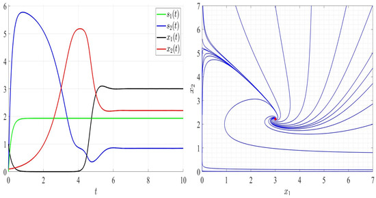
Figure 3. Comportment of system (2); the comportment of the components (left) and the $x_1-x_2$ comportment (right) for $D=5.9$. The red dot (right) is the equilibrium point in the plane ($x_1,x_2$).

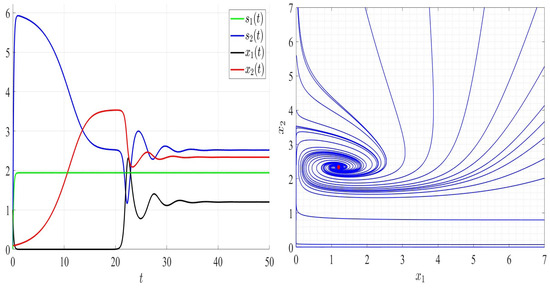
Figure 4. Comportment of system (2); the comportment of the components (left) and the $x_1-x_2$ comportment (right) for $D=6.8$. The red dot (right) is the equilibrium point in the plane ($x_1,x_2$).

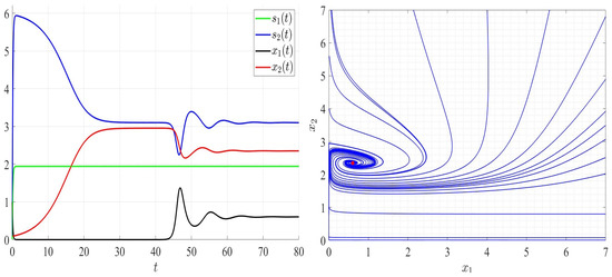
Figure 5. Comportment of system (2); the comportment of the components (left) and the $x_1-x_2$ comportment (right) for $D=6.9$. The red dot (right) is the equilibrium point in the plane ($x_1,x_2$).

In Figure 6, we chose $D=7$ satisfying Assumptions A1 to A6 but not Assumption A7. As can be seen, species 2 persists; however, species 1 goes to extinction and the global stability of the steady state $E^2$ (Figure 6, right). In Figure 7, $D=8$ and thus Assumptions A1 and A5 are not verified. Both competing bacteria go to extinction and then the trivial steady state $E^0$ is globally asymptotically stable. All solutions filling the positive cone converge to the point $(0,0)$ (Figure 7, right). By comparing Figure 3, Figure 4, Figure 5, Figure 6 and Figure 7, one can see that by increasing the dilution rate (D) values, the equilibrium point $E^{\ast }$ approaches slowly the steady state $E^2$ for a range of values of D; then, the steady state $E^2$ approaches the trivial steady state $E^0$ corresponding to the extinction of both bacteria.

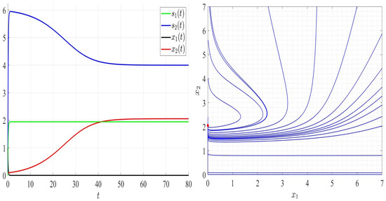
Figure 6. Comportment of system (2); the comportment of the components (left) and the $x_1-x_2$ comportment (right) for $D=7$. The red dot (right) is the equilibrium point in the plane ($x_1,x_2$).

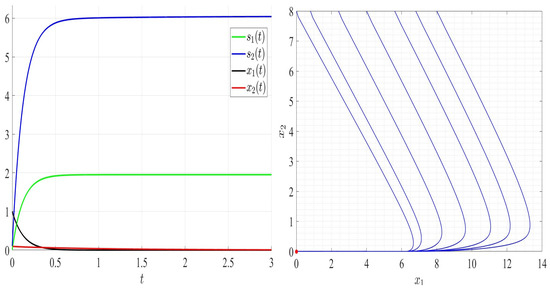
Figure 7. Comportment of system (2); the comportment of the components (left) and the $x_1-x_2$ comportment (right) for $D=8$. The red dot (right) is the equilibrium point in the plane ($x_1,x_2$).

7.2. Numerical Examples for the Control Problem

In the following examples, we assume that the control, r, is a time-varying function, $r\left(t\right)$, with bounds given by $r^{\min }=0.01$ and $r^{\max }=5$ and initial value $r\left(0\right)=0.05$. We consider an initial state value $x_0=(12,16,0.01,0.01)$ with final time $T=10$. The used numerical scheme for the control problem is given in Appendix A.

As it is seen in Figure 8, Figure 9 and Figure 10, the optimal solution is very smooth. The values of the control decrease if we increase the ${\kappa }_3$ values; however, they increase if we increase the values of ${\kappa }_1$ and ${\kappa }_2$. Note that the final values of the organic matter and the biomass are the same when changing the values of ${\kappa }_1$, ${\kappa }_2$, and ${\kappa }_3$. The optimal strategy allows to decrease the organic matter and optimise the control values (costs).

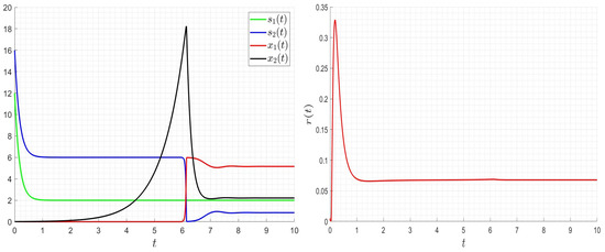
Figure 8. Influence of the optimal strategy on the dynamics for ${\kappa }_1=1$, ${\kappa }_2=1$, ${\kappa }_3=1$, $D=5.9$.

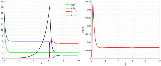
Figure 9. Influence of the optimal strategy on the dynamics for ${\kappa }_1=1$, ${\kappa }_2=1$, ${\kappa }_3=10$, $D=5.9$.

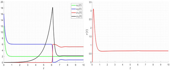
Figure 10. Influence of the optimal strategy on the dynamics for ${\kappa }_1=10$, ${\kappa }_2=10$, ${\kappa }_3=1$, $D=5.9$.

8. Conclusions

We studied a simple four-dimensional mathematical model describing an obligate one-way beneficial relationship from one species to the other one under perfect mixing conditions in the presence of the leachate recirculation. We considered a two-component nutriment whose soluble component is degraded by both competing species and the insoluble nutriment is exposed to a solubilisation process. We reduced the model to a planar one, we study the local and global stability, and then we applied Thieme’s results [48] to deduce the persistence of both competing bacteria. This result contradicts the competitive exclusion principle. Furthermore, we proposed an optimal control on the leachate recirculation with the aim to reduce the organic matter inside the chemostat with optimal operation costs. Finally, we provided several numerical tests confirming the obtained results.

The effect of leachate recycling can be considered in several bioreactor configurations, in particular the membrane bioreactor process for a wastewater treatment. Another possible extension of this study that can be considered in the future is to investigate the impact of the periodic dilution rate on increasing bacteria production, which leads to reducing the organic matter (both insoluble and soluble nutriments).

References

- Hsu, S.B.; Hubbell, S.; Waltman, P. A mathematical theory for single-nutrient competition in continuous cultures of micro-organisms. SIAM J. Appl. Math. 1977, 32, 366–383. [Google Scholar] [CrossRef]
- Butler, G.J.; Wolkowicz, G.S.K. A mathematical model of the chemostat with a general class of functions describing nutrient uptake. SIAM J. Appl. Math. 1985, 45, 138–151. [Google Scholar] [CrossRef]
- Wolkowicz, G.S.K.; Lu, Z. Global dynamics of a mathematical model of competition in the chemostat: General response functions and differential death rates. SIAM J. Appl. Math. 1992, 52, 222–233. [Google Scholar] [CrossRef]
- Smith, H.L.; Waltman, P. Competition for a single limiting resource in continuous culture: The variable-yield model. SIAM J. Appl. Math. 1994, 54, 1113–1131. [Google Scholar] [CrossRef]
- Smith, H.L.; Thieme, H.R. Chemostats and epidemics: Competition for nutrients/ hosts. Math. Biosci. Eng. 2013, 10, 1635–1650. [Google Scholar] [CrossRef]
- Korytowski, D.; Smith, H. Permanence and Stability of a Kill the Winner Model in Marine Ecology. Bull. Math. Biol. 2017, 79, 995–1004. [Google Scholar] [CrossRef]
- Browne, C.; Smith, H. Dynamics of virus and immune response in multi-epitope network. J. Math. Biol. 2018, 77, 1833–1870. [Google Scholar] [CrossRef]
- Wade, M.; Harmand, J.; Benyahia, B.; Bouchez, T.; Chaillou, S.; Cloez, B.; Godon, J.J.; Boudjemaa, B.M.; Rapaport, A.; Sari, T.; et al. Perspectives in mathematical modelling for microbial ecology. Ecol. Model. 2016, 321, 64–74. [Google Scholar] [CrossRef]
- Vandermeer, J.; Pascual, M. Competitive coexistence through intermediate polyphagy. Ecol. Complex. 2006, 3, 37–43. [Google Scholar] [CrossRef]
- Shyamsunder; Purohit, S. A novel study of the impact of vaccination on pneumonia via fractional approach. Partial Differ. Equ. Appl. Math. 2024, 10, 100698. [Google Scholar] [CrossRef]
- Shyamsunder; Purohit, S.D.; Suthar, D.L. A novel investigation of the influence of vaccination on pneumonia disease. Int. J. Biomath. 2024, online ready., 2450080. [Google Scholar] [CrossRef]
- Shyamsunder. Comparative Implementation of Fractional Blood Alcohol Model by Numerical Approach. Crit. Rev. Biomed. Eng. 2025, 53, 11–19. [Google Scholar] [CrossRef]
- Albargi, A.H.; El Hajji, M. Bacterial Competition in the Presence of a Virus in a Chemostat. Mathematics 2023, 11, 3530. [Google Scholar] [CrossRef]
- Sari, T. Commensalism and syntrophy in the chemostat: A unifying graphical approach. AIMS Math. 2024, 9, 18625–18669. [Google Scholar] [CrossRef]
- Hsu, S.B.; Waltman, P. Analysis of a model of two competitors in a chemostat with an external inhibitor. SIAM J. Appl. Math. 1991, 52, 528–540. [Google Scholar] [CrossRef]
- El Hajji, M. How can inter-specific interferences explain coexistence or confirm the competitive exclusion principle in a chemostat. Int. J. Biomath. 2018, 11, 1850111. [Google Scholar] [CrossRef]
- Grognard, F.; Mazenc, F.; Rapaport, A. Polytopic Lyapunov functions for the stability analysis of persistence of competing species. In Proceedings of the 44th IEEE Conference on Decision and Control, Seville, Spain, 15 December 2005. [Google Scholar] [CrossRef]
- Lobry, C.; Mazenc, F.; Rapaport, A. Persistence in ecological models of competition for a single resource. C.R. Acad. Sci. Paris Ser. I 2004, 340, 199–240. [Google Scholar] [CrossRef]
- Lobry, C.; Harmand, J. A new hypothesis to explain the coexistence of n species in the presence of a single resource. C. R. Biol. 2006, 329, 40–46. [Google Scholar] [CrossRef]
- Mazenc, F.; Lobry, C.; Rapaport, A. Persistence in Ratio-Dependent Models of Consumer-Resource Dynamics. In Proceedings of the Sixth Mississippi State—UAB Conference on Differential Equations & Computational Simulations, Strakville, MI, USA, 13–15 May 2005. [Google Scholar]
- Alsolami, A.A.; El Hajji, M. Mathematical Analysis of a Bacterial Competition in a Continuous Reactor in the Presence of a Virus. Mathematics 2023, 11, 883. [Google Scholar] [CrossRef]
- Bergstrom, C.T.; Bronstein, J.L.; Bshary, R.; Connor, R.C.; Daly, M.; Frank, S.A.; Gintis, H.; Keller, L.; Leimar, O.; Noe, R.; et al. Interspecific Mutualism: Puzzles and Predictions. In Genetic and Cultural Evolution of Cooperation; Hammerstein, P., Ed.; MIT Press: Cambridge, MA, USA, 2003; pp. 241–256. [Google Scholar]
- Boucher, D.H. The Biology of Mutualism: Ecology and Evolution; Oxford University Press: New York, NY, USA, 1985. [Google Scholar]
- Zientz, E.; Dandekar, T.; Gross, R. Metabolic Interdependence of Obligate Intracellular Bacteria and Their Insect Hosts. Microbiol. Mol. Biol. Rev. 2004, 68, 745–770. [Google Scholar] [CrossRef]
- Margulis, L. Origin of Eukaryotic Cells; Yale University Press: New Haven, CT, USA, 1970. [Google Scholar]
- Mereschkowsky, C. Uber Natur and Ursprung der Chromatophoren im Pflanzenreiche. Biol. Zentralbl. 1905, 25, 593–604. [Google Scholar]
- Cook, J.M.; Rasplus, J.Y. Mutualists with attitude: Coevolving fig wasps and figs. Trends Ecol. Evol. 2003, 18, 241–248. [Google Scholar] [CrossRef]
- Corsaro, D.; Venditti, D.; Padula, M.; Valassina, M. Intracellular life. Crit. Rev. Microbiol. 1999, 25, 39–79. [Google Scholar] [CrossRef]
- Hata, H.; Kato, M. A novel obligate cultivation mutualism between damselfish and Polysiphonia algae. Biol. Lett. 2006, 2, 593–596. [Google Scholar] [CrossRef]
- Pellmyr, O.; Leebens-Mack, J. Forty million years of mutualism: Evidence for Eocene origin of the yucca-yucca moth association. Proc. Natl. Acad. Sci. USA 1999, 96, 9178–9183. [Google Scholar] [CrossRef]
- Rowan, R.; Knowlton, N.; Baker, A.; Jara, J. Landscape ecology of algal symbiont communities explains variation in episodes of coral bleaching. Nature 1997, 338, 265–269. [Google Scholar] [CrossRef]
- Wernegreen, J.J. Genome evolution in bacterial endosymbionts of insects. Nat. Rev. Genet. 2002, 3, 850–861. [Google Scholar] [CrossRef]
- Wilson, E.O. Social Symbiosis. In Sociobiology: The New Synthesis, 25th Anniversary ed.; Harvard University Press: Cambridge, MA, USA, 1975; p. 354. [Google Scholar] [CrossRef]
- Giannis, A.; Makripodis, G.; Simantiraki, F.; Somara, M.; Gidarakos, E. Monitoring operational and leachate characteristics of an aerobic simulated landfill bioreactor. Waste Manag. 2008, 28, 1346–1354. [Google Scholar] [CrossRef]
- Benbelkacem, H.; Bayard, R.; Abdelhay, A.; Zhang, Y.; Gourdon, R. Effect of leachate injection modes on municipal solid waste degradation in anaerobic bioreactor. Bioresour. Technol. 2010, 101, 5206–5212. [Google Scholar] [CrossRef]
- Bilgili, M.S.; Demir, A.; Özkaya, B. Influence of leachate recirculation on aerobic and anaerobic decomposition of solid wastes. J. Hazard. Mater. 2007, 143, 177–183. [Google Scholar] [CrossRef]
- Hussein, O.A.; Ibrahim, J.A.A. Leachates Recirculation Impact on the Stabilization of the Solid Wastes—A Review. J. Ecolog. Eng. 2023, 24, 172–183. [Google Scholar] [CrossRef]
- Francois, V.; Feuillade, G.; Matejka, G.; Lagier, T.; Skhiri, N. Leachate recirculation effects on waste degradation: Study on columns. Waste Manag. 2007, 27, 1259–1272. [Google Scholar] [CrossRef] [PubMed]
- Bisi, M.; Groppi, M.; Martaló, G.; Travaglini, R. Optimal control of leachate recirculation for anaerobic processes in landfills. Discret. Contin. Dyn. Syst.-B 2021, 26, 2957–2976. [Google Scholar] [CrossRef]
- Laraj, O.; El Khattabi, N.; Rapaport, A. Mathematical model of anaerobic digestion with leachate recirculation. In Proceedings of the CARI 2022, Sophia Antipolis, France, 4–7 October 2022. [Google Scholar]
- El Hajji, M. Mathematical modeling for anaerobic digestion under the influence of leachate recirculation. AIMS Math. 2023, 8, 30287–30312. [Google Scholar] [CrossRef]
- El Hajji, M.; Al-Subhi, A.Y.; Alharbi, M.H. Mathematical investigation for two-bacteria competition in presence of a pathogen with leachate recirculation. Int. J. Anal. Appl. 2024, 22, 45. [Google Scholar] [CrossRef]
- El Hajji, M. Influence of the presence of a pathogen and leachate recirculation on a bacterial competition. Int. J. Biomath. 2024, online ready, 2450029. [Google Scholar] [CrossRef]
- Smith, H.L.; Waltman, P. Cambridge Studies in Mathematical Biology. In The Theory of the Chemostat. Dynamics of Microbial Competition; Cambridge University Press: Cambridge, UK, 1995; Volume 13. [Google Scholar] [CrossRef]
- Monod, J. Croissance des populations bactériennes en fonction de la concentration de l’aliment hydrocarboné. C. R. Acad. Sci. 1941, 212, 771–773. [Google Scholar]
- Lobry, J.R.; Flandrois, J.P.; Carret, G.; Pave, A. Monod’s bacterial growth revisited. Bull. Math. Biol. 1992, 54, 117–122. [Google Scholar] [CrossRef]
- Hsu, S.B. Ordinary differential equations with applications. Ser. Appl. Math. 2005, 16, 256. [Google Scholar] [CrossRef]
- Thieme, H.R. Convergence results and a Poincaré-Bendixson trichotomy for asymptotically autonomous differential equations. J. Math. Biol. 1992, 30, 755–763. [Google Scholar] [CrossRef]
- Fleming, W.; Rishel, R. Deterministic and Stochastic Optimal Control; Springer: New York, NY, USA, 1975. [Google Scholar] [CrossRef]
- Lenhart, S.; Workman, J.T. Optimal Control Applied to Biological Models; Chapman and Hall: London, UK, 2007. [Google Scholar] [CrossRef]
- Pontryagin, L.S.; Boltyanskii, V.G.; Gamkrelidze, R.V.; Mishchenko, E.F.; Trirogoff, K.N.; Neustadt, L.W. The Mathematical Theory of Optimal Processes; CRC Press: Boca Raton, FL, USA, 2000. [Google Scholar] [CrossRef]
Disclaimer/Publisher’s Note: The statements, opinions and data contained in all publications are solely those of the individual author(s) and contributor(s) and not of MDPI and/or the editor(s). MDPI and/or the editor(s) disclaim responsibility for any injury to people or property resulting from any ideas, methods, instructions or products referred to in the content. |
© 2024 by the authors. Licensee MDPI, Basel, Switzerland. This article is an open access article distributed under the terms and conditions of the Creative Commons Attribution (CC BY) license (https://creativecommons.org/licenses/by/4.0/).