Article

Synergistic Impact of Active Case Detection and Early Hospitalization for Controlling the Spread of Yellow Fever Outbreak in Nigeria: An Epidemiological Modeling and Optimal Control Analysis

by
Nawaf L. Alsowait
1,
Mohammed M. Al-Shomrani
2,*,
Ismail Abdulrashid
3 and
Salihu S. Musa
4,5,6,7,*
1
Department of Mathematics, College of Science, Northern Border University, Arar 91431, Saudi Arabia
2
Department of Mathematics, Faculty of Science, King Abdulaziz University, Jeddah 21589, Saudi Arabia
3
School of Finance and Operations Management, The University of Tulsa, Tulsa, OK 74104, USA
4
Department of Genomics and Computational Biology, University of Massachusetts Chan Medical School, Worcester, MA 01605, USA
5
Department of Mathematics, Aliko Dangote University of Science and Technology, Wudil 713101, Kano, Nigeria
6
Department of Mathematics, University of Maryland, College Park, MD 20742, USA
7
Institute for Health Computing, University of Maryland, North Bethesda, MD 20852, USA
*
Authors to whom correspondence should be addressed.
Mathematics 2024, 12(23), 3817; https://doi.org/10.3390/math12233817
Submission received: 13 August 2024 / Revised: 4 November 2024 / Accepted: 14 November 2024 / Published: 2 December 2024
(This article belongs to the Special Issue Mathematical Analysis of Infectious Disease)

Abstract

:
Capturing the factors influencing yellow fever (YF) outbreaks is essential for effective public health interventions, especially in regions like Nigeria, where the disease poses significant health risks. This study explores the synergistic effects of active case detection (ACD) and early hospitalization on controlling YF transmission dynamics. We develop a dynamic model that integrates vaccination, active case detection, and hospitalization to enhance our understanding of disease spread and inform prevention strategies. Our methodology encompasses mechanistic dynamic modeling, optimal control analysis, parameter estimation, model fitting, and sensitivity analyses to study YF transmission dynamics, ensuring the robustness of control measures. We employ advanced mathematical techniques, including next-generation matrix methods, to accurately compute the reproduction number and assess outbreak transmissibility. Rigorous qualitative analysis of the model reveals two equilibria: disease-free and endemic, demonstrating global asymptotic stability and its impact on overall YF transmission dynamics, significantly affecting control and prevention mechanisms. Furthermore, through sensitivity analysis, we identify crucial parameters of the model that require urgent attention for more effective YF control. Moreover, our results highlight the critical roles of ACD and early hospitalization in reducing YF transmission. These insights provide a foundation for informed decision making and resource allocation in epidemic control efforts, ultimately contributing to the enhancement of public health strategies aimed at mitigating the impact of YF outbreaks.

1. Introduction

Yellow fever (YF) is a viral disease transmitted primarily by mosquitoes, specifically the Aedes aegypti species in urban areas and Haemagogus and Sabethes species in jungle regions [1,2,3,4]. This disease poses a significant threat to public health and socioeconomic stability, particularly in tropical and subtropical regions such as Africa, Central America, and South America (WHO, November 2019). While YF has been largely controlled through extensive vaccination campaigns in some endemic nations [1,4], it continues to be a concern due to its potential to cause large outbreaks.
Nigeria, being a country at risk for YF outbreaks, is a key focus under the 2017-launched Eliminate Yellow Fever Epidemics (EYE) strategy by the World Health Organization (WHO). This strategy aims to assist 40 high-risk countries, primarily in Africa and the Americas, in detecting, preventing, and responding to YF case scenarios with the goal of protecting more than 1 billion individuals at risk of YF infection [5].
Vaccination remains the most effective method for preventing and controlling YF transmission [1,4,6,7]. A single dose of the YF vaccine confers lifelong immunity and protection against the disease, with a high efficacy rate within ten days and reaching over 99% effectiveness within thirty days [4,5]. However, challenges exist in achieving sufficient vaccination coverage. In Nigeria, the national immunization coverage for YF in 2020 was only 54%, below the herd immunity threshold of 80% required to prevent outbreaks [5]. Besides vaccination, early hospitalization with adequate supportive care improves survival rates for YF patients as there are currently no specific antiviral drugs for the disease [1,5]. Targeted vector control measures, particularly in urban areas where Aedes aegypti mosquitoes are prevalent, are also crucial for preventing YF spread [5].
Mathematical modeling and analysis have been instrumental in understanding the dynamics of YF transmission. Various studies have utilized those kinds of models to analyze the impact of vaccination, transmission dynamics, and intervention strategies for YF outbreaks [8,9,10,11,12,13,14,15,16,17,18,19]. For instance, Zhao et al. (2018) analyzed the impact of vaccination on a large-scale YF outbreak in Angola, emphasizing the importance of timely vaccination in preventing new cases and deaths [4]. Kung’aro et al. (2015) developed a model to investigate YF transmission dynamics in human and primate populations, highlighting the role of continuous vaccination due to waning immunity [2]. Monath and Vasconcelos (2014) studied clinical and epidemiological aspects of YF, emphasizing the importance of early vaccination in combating epidemics [3]. Despite vaccination efforts, YF outbreaks persist, necessitating robust modeling frameworks to assess transmission dynamics and optimize control strategies. Mathematical models play a pivotal role in disease prevention and control, integrating factors such as vaccination coverage, vector control, human behavior, and awareness programs to estimate outbreak burdens and inform policy decisions [4,20,21,22]. Existing YF models often lack comprehensiveness or interpretability, posing challenges for healthcare decision makers [4,5]. This study addresses these gaps by developing an explainable epidemic model tailored for assessing YF transmission dynamics in Nigeria. Our model integrates vaccination, quarantine, treatment, and active case detection (ACD) into a unified framework, enabling a holistic evaluation of intervention strategies and their impacts on disease spread [4,5]. We employ rigorous mathematical analysis [8], optimal control theory [23], parameter estimation [17], and sensitivity analyses [9] to ensure robustness and reliability.
Our study advances YF epidemiology by providing a comprehensive tool tailored to Nigerian contexts, building upon and extending previous research [2,3,4]. By integrating diverse control strategies and applying rigorous analytical techniques, we elucidate YF transmission dynamics and identify critical parameters like the basic reproduction number ( R 0 ) [17]. This approach not only fills gaps in the current literature but also offers practical insights for optimizing YF control strategies in endemic regions [23,24]. Our main objectives include developing a detailed dynamic model to simulate YF spread under various scenarios, using optimal control theory to identify effective interventions, and validating our model with real-world data [24]. Sensitivity analyses will further enhance our understanding of parameter influences on disease dynamics. Ultimately, this study contributes essential knowledge for informed decision making in YF epidemic control efforts, ensuring effective public health responses. The subsequent sections of this manuscript following this introductory section will detail the methodology, mathematical analysis, model fitting, and discussion of results, providing comprehensive insights for informed decision making in epidemic control efforts.

2. Methods

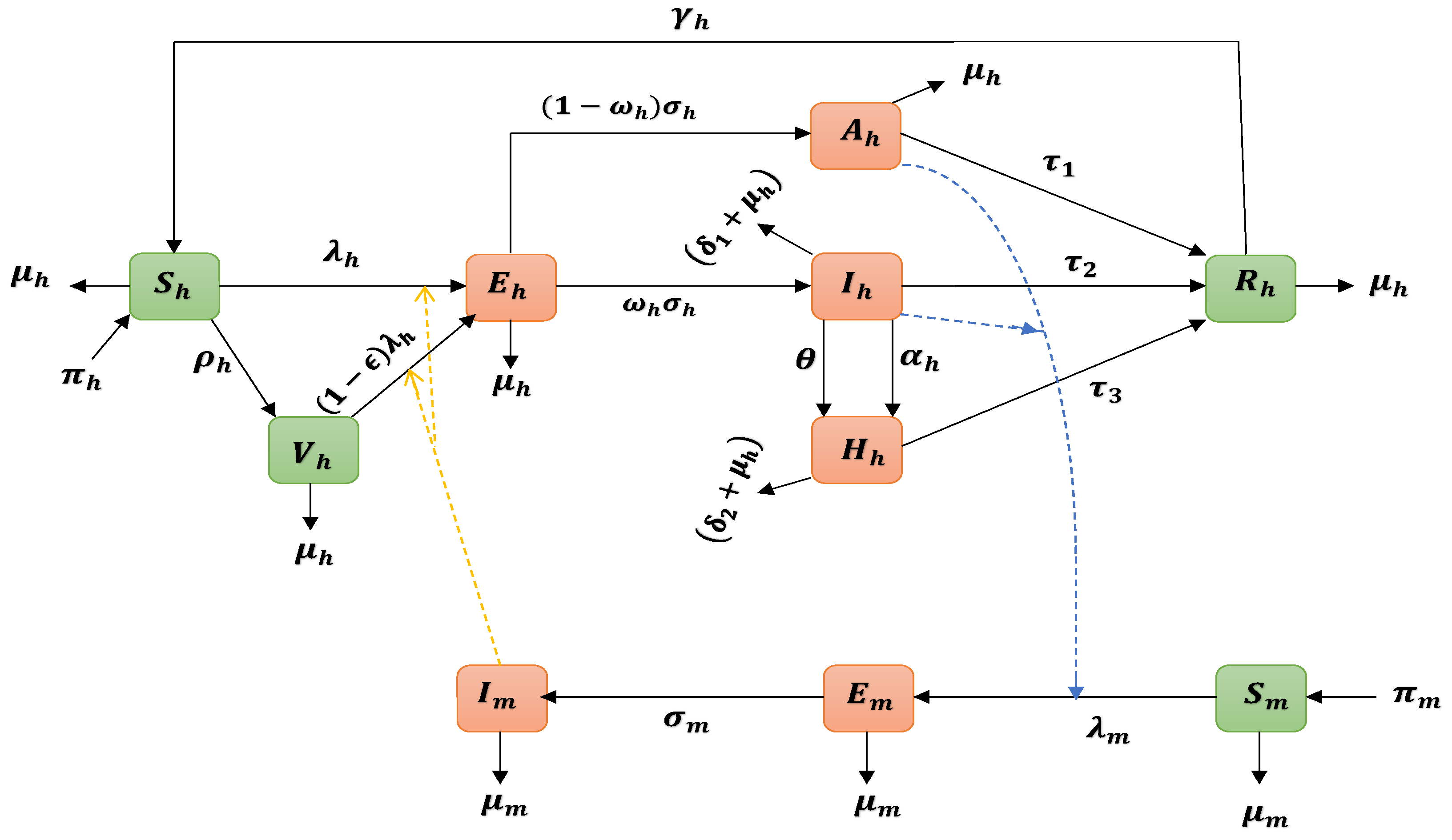
2.1. Yellow Fever Epidemic Model

This study employs a Susceptible–Exposed–Infectious–Recovered (SEIR)-based model, a standard framework for evaluating the epidemiological impact of interventions like isolation and active case detection on YF transmission at a community level. The objective is to develop an explainable epidemic model that provides insights into the dynamics of YF transmission. To construct this model, we utilize time-series epidemiological data on YF cases from the Nigeria Center for Disease Control (NCDC) surveillance report [25]. The population is categorized into seven subgroups based on their status: susceptible ( S h ( t ) ), vaccinated ( V h ( t ) ), exposed ( E h ( t ) ), asymptomatically infected ( A h ( t ) ), symptomatically mild infected ( I m ( t ) ), symptomatically severe infected ( I s ( t ) ), and isolated or hospitalized infected ( H m ( t ) ), along with those who have recovered or been removed from the infectious pool ( R h ( t ) ). This segmentation allows us to capture the complex interactions and dynamics of YF transmission within the population over time. The SEIR model framework incorporates parameters that govern the transitions between these population subgroups, such as the transmission rate, incubation period, recovery rate, and effectiveness of interventions like isolation and active case detection. These parameters are estimated or derived based on epidemiological data and literature insights, ensuring the model’s accuracy and relevance to real-world scenarios. By simulating the dynamics of YF transmission within this structured framework, we aim to assess the effectiveness of various control measures and intervention strategies in curbing the spread of YF. The model’s transparency and explainability make it a valuable tool for informing public health policies and guiding decision-making processes to combat YF outbreaks effectively.
N h ( t ) = S h ( t ) + V h ( t ) + E h ( t ) + A h ( t ) + I m ( t ) + I s ( t ) + R h ( t ) .
There are three subgroups within the overall population of mosquitoes at time t, denoted by the symbol N m ( t ) : susceptible ( S m ( t ) ), exposed ( E m ( t ) , and infectious ( I m ( t ) ). Hence,
N m ( t ) = S m ( t ) + E m ( t ) + I m ( t ) .
The YF model (Figure 1) and the variables (Table 1) with model parameters (Table 2) satisfy the following non-linear systems of ordinary differential equations, given by,
d S h dt = π h + γ h R h λ h S h ( ρ h + μ h ) S h , d V h dt = ρ h S h ( 1 ϵ ) λ h V h μ h V h d E h dt = λ h [ S h + ( 1 ϵ ) V h ] ( σ h + μ h ) E h , d A h dt = ( 1 ω h ) σ h E h ( τ 1 + μ h ) A h , d I h dt = ω h σ h E h ( θ + α h ) I h ( δ 1 + τ 2 + μ h ) I h , d H h dt = ( θ + α h ) I h ( δ 2 + τ 3 + μ h ) H h , d R h dt = τ 1 A h + τ 2 I h + τ 3 H h ( γ h + μ h ) R h , d S m dt = π m λ m S m μ m S m , d E m dt = λ m S m ( σ m + μ m ) E m , d I m dt = σ m E m μ m I m .
Here, the forces of infections of humans and mosquitoes are, respectively, given by,
λ h = b β m h I m N h and λ m = b β h m ( ψ A h + I h ) N h ,
where N h = S h + V h + E h + A h + I h + H h + R h and N m = S m + E m + I m , respectively, represent the total population of humans and mosquitoes.
Figure 1. Schematic representation of the Yellow Fever Virus (YFV) transmission model. The population is delineated into seven distinct compartments based on their infection status: susceptible ( S h ( t ) ), vaccinated ( V h ( t ) ), exposed ( E h ( t ) ), asymptomatically infected ( A h ( t ) ), symptomatically mild infected ( I m ( t ) ), symptomatically severe infected ( I s ( t ) ), and isolated or hospitalized infected ( H m ( t ) ). Additionally, individuals who have recovered or been removed from the infectious pool are denoted as R h ( t ) . This compartmentalization enables a comprehensive analysis of the complex interactions and dynamics of YFV transmission within the population over time. The green nodes represent the uninfected classes, while the orange nodes indicate the infected classes, thereby illustrating the various pathways and outcomes associated with the infection.
Mathematics 12 03817 g001
Table 1. Definition of the model’s state variables.
VariableDescription
N h Total human population
S h Susceptible humans who are at risk of contracting the YFV
V h Population of vaccinated susceptible humans against YFV infection
E h Population of humans exposed to YFV
A h Population of asymptomatically infected humans with YFV
I h Population of symptomatically infected humans with YFV
H h Population of hospitalized/isolated humans
R h Population of recovered humans
N m Total mosquito population
S m Population of susceptible mosquitoes
E m Population of mosquitoes exposed to YFV
I m Population of YFV-infected mosquitoes
Table 2. Description of parameters of model (1).
ParameterInterpretation/Description
π h Recruitment rate of humans
π m Recruitment rate of mosquitoes
μ h Natural death rate of humans
β m h Transmission probability from infectious mosquitoes to susceptible humans
bMosquito biting rate
ψ Modification parameter for the decrease in infectiousness of A h
ρ h Vaccination rate
ϵ Vaccine efficacy
ω h Fraction of humans exposed to YFV
σ h Rate of exposed humans becoming infected humans
α h Hospitalization rate
θ Rate of active case detection
δ l ( l = 1 , 2 ) YFV-induced death rate
τ k ( k = 1 , 2 , 3 ) Recovery rate of infected humans
γ h Rate of immunity loss
π m Recruitment rate of mosquitoes
μ m Mosquito natural death rate
β h m Probability of transmission from infected humans to susceptible mosquitos
σ m Rate of exposed mosquitoes becoming infected mosquitoes
mAverage mosquito to human ratio
In our model, denoted as (1), we assume all state parameters to be strictly positive, reflecting the real-world scenario of disease dynamics. Specifically, the parameter ordering τ 3 < τ 2 < τ 1 signifies that the recovery rate is higher in the asymptomatic stage compared to the symptomatically infected and hospitalized phases. This assumption aligns with the understanding that the disease is less severe in the asymptomatic stage, leading to a faster recovery [4]. We simplify our model by grouping all symptomatically hospitalized individuals, including those in mild, severe, and toxic stages, into a single compartment denoted as H h . The toxic phase, characterized by the absence of viremia (presence of YFV in blood), indicates a non-infectious state [4]. However, this phase has a higher case fatality rate (CFR) due to systemic organ infections, such as the kidneys and liver, often resulting in death within 7–10 days [26]. According to [4,26], the symptomatically infected stage exhibits higher transmissibility compared to the asymptomatic stage, denoted by the parameter 0 < ψ < 1 in our model. This parameter captures the relative decrease in transmissibility of infected individuals, reflecting the dynamics of YF transmission within the population. In (1), several key parameters govern the interactions and dynamics of YF transmission. The recruitment rates of humans ( π h ) and mosquitoes ( π m ), along with the YF infection rates ( λ h and λ m ) from infectious mosquitoes to susceptible humans and vice versa, are crucial factors. The parameter b represents the mosquito’s biting rate per unit time. Additionally, β i ( i = m h , h m ) signifies the probability of YF infection per mosquito bite, with ψ capturing the modification in transmissibility due to infection. The vaccination parameter ρ accounts for the ratio of susceptible humans receiving vaccination, assuming a single dose provides lifelong immunity [26]. Vaccinated individuals can still acquire infection at a reduced rate ( 1 ϵ ) λ h , where ϵ denotes vaccine efficacy, which can be up to 100% [26]. Other parameters such as σ h (rate of symptom development), ω (fraction moving to symptomatic stage), τ k (recovery rates), δ l (YF-induced death rates), γ h (loss of immunity post-recovery), α h (hospitalization rate), and t h e t a (ACD rate) play crucial roles in modeling disease progression and intervention effectiveness. For mosquitoes, we consider a simple Susceptible–Exposed–Infected model, with parameters π m (mosquito recruitment), λ m (YF infection rate), and μ m (mosquito natural death rate). We assume that hospitalized/isolated individuals do not transmit YFV due to their controlled environment and medical attention, emphasizing their non-infectious status.

2.2. Model’s Preliminary Qualitative Properties

By taking into account the two equations below for the rate of change of the total human N h ( t ) and mosquito N m ( t ) populations over time, we will first analyze the fundamental dynamic features of the model (1); thus
N h ( t ) = d N h dt = π h μ h N h δ 1 I h δ 2 H h π h μ h N h ,
and
N m ( t ) = d N m dt = π m μ m N m ,
where prime (′) in the above equations denotes the derivative with respect to time, t.
Furthermore, considering the region,
Ω = ( S h , V h , E h , A h , I h , H h , R h , S m , E m , I m ) R + 10 : N h π h μ h , N m π m μ m .
Upon solving Equations (3) and (4) for the variables N h and N m , it can be demonstrated that all solutions originating within the region Ω will remain within Ω for all time t with t 0 . This property establishes Ω as a positively invariant region, indicating that it is sufficient to analyze solutions confined to Ω to understand the system’s behavior. The mathematical rigor supporting the existence, uniqueness, and continuity of solutions within this region is detailed in [27], providing a solid foundation for our analysis.

3. Theoretical Analysis

3.1. Disease-Free Equilibrium and Basic Reproduction Number

The basic reproduction number, denoted as R 0 , holds paramount significance in epidemiological modeling as it quantifies the potential spread of an infectious disease within a susceptible population. Specifically, R 0 signifies the average number of secondary cases generated by a single infected individual introduced into an entirely susceptible community throughout their infectious period. In our analysis, the computation of R 0 is conducted utilizing the next-generation matrix technique, as described in works by Diekmann and Heesterbeek [28,29]. This technique has been widely adopted in previous epidemiological research studies, showcasing its reliability and applicability in assessing disease transmission dynamics. Notable contributions utilizing the next-generation matrix technique include studies by Chowell et al. [30], Yang and Gao [31], and Musa et al. [32], underscoring its importance and acceptance within the scientific community. To compute R 0 for YFV transmission, we first determine the model’s steady-state disease-free equilibrium (DFE), which in this case is provided by
Ω 0 = S h 0 , V h 0 , E h 0 , A h 0 , I h 0 , H h 0 , R h 0 , S m 0 , E m 0 , I m 0 = π h ρ h + μ h , π h ρ h ( ρ h + μ h ) μ h , 0 , 0 , 0 , 0 , 0 , π m μ m , 0 , 0 .
For the model (1), the linear stability of the DFE is determined following the next-generation matrix framework [29]. Let the matrices F 1 and F 2 representing the fraction of the new infection terms and the remaining transfer terms, respectively, be given by
F 1 = 0 0 0 0 0 A 1 0 0 0 0 0 0 0 0 0 0 0 0 0 0 0 0 0 0 0 A 2 A 3 0 0 0 0 0 0 0 0 0 , and F 2 = q 1 0 0 0 0 0 q 0 σ h q 2 0 0 0 0 ω h σ h 0 q 3 + q 4 0 0 0 0 0 q 3 q 5 0 0 0 0 0 0 q 6 0 0 0 0 0 σ m μ m .
Direct calculation yields
F 2 1 = q 1 1 0 0 0 0 0 q 0 σ h q 1 q 2 q 2 1 0 0 0 0 ω h σ h q 1 q 3 + q 4 0 q 3 + q 4 1 0 0 0 q 3 ω h σ h q 1 q 3 + q 4 q 5 0 q 3 q 3 + q 4 q 5 q 5 1 0 0 0 0 0 0 q 6 1 0 0 0 0 0 σ m q 6 μ m μ m 1 ,
and
F 1 · F 2 1 = 0 0 0 0 A 1 σ m q 6 μ m A 1 μ m 0 0 0 0 0 0 0 0 0 0 0 0 0 0 0 0 0 0 A 2 q 0 σ h q 1 q 2 + A 3 ω h σ h q 1 q 3 + q 4 A 2 q 2 A 3 q 3 + q 4 0 0 0 0 0 0 0 0 0 .
where A 1 = V h 0 q 7 + S h 0 b μ h β mh π h , A 2 = μ h b β hm S m 0 ψ π h , and A 3 = μ h b β hm S m 0 π h . With ρ representing the spectral radius of the next-generation matrix, q 0 = 1 ω h , q 1 = σ h + μ h , q 2 = τ 1 + μ h , q 3 = θ + α h , q 4 = δ 1 + τ 2 + μ h , q 5 = δ 2 + τ 3 + μ h , q 6 = σ m + μ m , q 7 = 1 ϵ , q 8 = γ h + μ h , and q 9 = ρ h + μ h , and substituting Equations (5)–(7) into R 0 = ρ ( F 1 F 2 1 ) , we obtain R 0 as follows
R 0 = ρ ( F 1 F 2 1 ) = R 0 h · R 0 m ,
where
R 0 h = b β m h μ h π h · q 7 ρ h + μ h q 9 · σ h q 1 q 0 ψ q 2 + ω h ( q 3 + q 4 ) , and R 0 m = b β h m σ m S m 0 q 6 μ m .
so that
R 0 = π h q 1 q 2 q 6 q 9 q 3 + q 4 π m β hm β mh μ h σ h σ m q 3 + q 4 q 0 ψ + ω h q 2 q 7 ρ h + μ h b π h q 1 q 2 q 6 q 9 q 3 + q 4 μ m ,
R 0 Interpretation
The epidemiological interpretation of the basic reproduction number, R 0 , given in Equation (8), is as follows:
i.
The term b β h m σ m S m 0 q 6 μ m represents the rate at which new mosquitoes become infected due to contact with an infected human host during the host’s period of exposure to the YFV. Here, b is the rate at which mosquitoes bite humans, β h m is the probability of YFV transmission from humans to mosquitoes per contact, σ m is the rate at which mosquitoes become infectious after acquiring the virus, S m 0 is the initial population of susceptible mosquitoes, q 6 is a model parameter related to the mosquito population dynamics, and μ m is the natural death rate of mosquitoes.
ii.
The expression b β m h μ h π h represents the rate of new human hosts becoming infected due to contact with a diseased mosquito during the mosquito’s expected infectious period. Here, b is the biting rate of mosquitoes, β m h is the probability of YFV transmission from mosquitoes to humans per contact, μ h is the natural death rate of humans, and π h is the recruitment rate of humans into the susceptible population.
iii.
The term σ h q 1 signifies the average duration of the infectious stage for humans, where σ h is the rate at which infected individuals develop clinical symptoms of YF, and q 1 is a model parameter related to the duration of the infectious period.
iv.
The expression q 7 ρ h + μ h q 9 represents the probability of vaccinated humans transitioning to the exposed class, with ρ h being the vaccination ratio of susceptible humans, q 7 related to vaccination dynamics, μ h the natural death rate of humans, and q 9 a model parameter associated with transitions between compartments.
v.
The term q 0 ψ q 2 indicates the likelihood that an individual, after exposure to YFV, survives the asymptomatic infectious stage before moving into the recovery class. Here, q 0 and q 2 are model parameters related to the progression of the disease and recovery.
vi.
The expression ω h q 3 + q 4 calculates the probability that an individual exposed to YFV survives the symptomatic infectious stage and transitions into the recovery class, facilitated by ACD. ω h represents the fraction of individuals progressing to recovery, while q 3 and q 4 are model parameters associated with disease progression and recovery facilitated by interventions.
To analyze the local stability of the DFE of the model (1), we adopted the method proposed by Vanden and Watmough [29] and obtained the following result:
Theorem 1. 
The DFE of the model (1) is locally asymptotically stable (LAS) whenever R 0 < 1 and unstable if R 0 > 1 .
The epidemiological implication derived from the result preceding Theorem 1 is profound. It indicates that a minor introduction of YF infection is unlikely to trigger a significant outbreak if the basic reproduction number ( R 0 ) is less than one ( R 0 < 1 ). This observation underscores the critical threshold R 0 = 1 , beyond which the potential for sustained transmission increases significantly. It is important to recognize that achieving R 0 < 1 is a crucial condition for mitigating YF according to epidemiological models, such as the one represented by Equation (1). However, this condition is sufficient but not necessary for YF control and eradication. Van den Driessche [29] emphasizes this point, indicating that while reducing R 0 below one is a step towards disease control, complete eradication requires sustained efforts to maintain R 0 levels below one over time. Furthermore, the persistence or eradication of YF hinges on the careful management of susceptible human recruitment and the implementation of effective control measures. Neglecting appropriate control strategies can exacerbate the spread of the disease, even if R 0 initially falls below one, highlighting the importance of continuous vigilance and intervention strategies in disease management.

3.2. Endemic Equilibrium

In this subsection, we aimed to investigate the existence of the model equilibrium points in dependence on the incidence functions. The endemic equilibrium (EE) points of the model (1) defined by
Ω * = ( S h * , V h * , E h * , A h * , I h * , H h * , R h * , S m * , E m * , I m * ) ,
in terms of the forces of infection, λ h * and λ m * , are computed below
S h * = τ 2 γ h ω h σ h E h + q 8 π h q 3 + q 4 q 2 + q 0 τ 1 γ h σ h E h q 3 + q 4 q 5 + E h γ h ω h q 2 q 3 σ h τ 3 q 8 q 2 q 5 q 3 + q 4 λ h + q 9 , V h * = 1 q 7 λ h + μ h ρ h λ h + q 9 σ h E h q 5 q 3 + q 4 τ 1 q 0 + q 2 q 5 τ 2 ω h + q 2 τ 3 q 3 ω h γ h q 8 q 2 q 5 q 3 + q 4 + π h + π h , A h * = q 0 σ h E h q 2 , I h * = ω h σ h E h q 3 + q 4 , H h * = q 3 ω h σ h E h q 5 q 3 + q 4 , R h * = σ h E h q 5 q 3 + q 4 τ 1 q 0 + q 2 q 5 τ 2 ω h + q 2 τ 3 q 3 ω h q 8 q 2 q 5 q 3 + q 4 , S m * = π m λ m + μ m , E m * = π m λ m q 6 ( λ m + μ m ) , and I m * = σ m π m λ m q 6 μ m ( λ m + μ m ) .
Substituting the above EE points (9) into Equation (2), we have
a 4 λ h 4 + a 3 λ h 3 + a 2 λ h 2 + a 1 λ h + a 0 = 0 .
For coefficients of the above polynomial (10), see Appendix A.
Following [23,33], we employed Descartes’ rule of sign changes on Equation (7) and list 32 various possibilities for the positive real roots of the polynomial (10) in Appendix B, Table A1, below.

3.3. Stability Analysis of the Endemic Equilibrium

In this study, we validate the global stability of the Endemic Equilibrium (EE) using Lyapunov function theory and LaSalle’s invariance principle [34,35]. These techniques have been extensively applied in prior research to analyze and confirm the global asymptotic stability of equilibrium points in epidemiological models [31,36]. By defining conditions under which trajectories of a dynamical system converge to a stable set—even when the system is not globally asymptotically stable—LaSalle’s invariance principle enhances Lyapunov’s theory. When examining complicated systems with non-linear dynamics, like epidemiological models, this principle is especially helpful. We ensure a rigorous investigation of the stability of the EE by using these mathematical methods in conjunction with established procedures in epidemiological modeling. We contribute to the robustness and dependability of our findings about the global stability of the EE in the context of YF transmission dynamics by utilizing Lyapunov function theory and LaSalle’s invariance principle.
Following previous works [31,36], we established the following result.
Theorem 2. 
The EE, E * , is globally asymptotically stable (GAS) in Ω * whenever R 0 > 1 and the following conditions are satisfied:
( 1 λ h λ h * ) ( 1 A h λ h * A h * λ h ) 0 , ( 1 λ h λ h * ) ( 1 I h λ h * I h * λ h ) 0 , ( 1 λ m λ m * ) ( 1 I m λ m * I m * λ m ) 0 , a n d ( I h I h * + ln H h H h * ) ( ln I h I h * + A h A h * ) .
The proof for the aforementioned Theorem 2 is provided in Appendix C.

3.4. Optimal Control Analysis

In this section, we introduce two control functions, denoted as u 1 ( t ) for active case detection and u 2 ( t ) for hospitalization, into our model. The objective is to minimize the number of asymptotically infected individuals with YF, reduce the population requiring hospitalization or isolation, and optimize the cost associated with these control measures. Our focus is on identifying the optimal values of u 1 ( t ) and u 2 ( t ) that achieve these goals efficiently and effectively within the epidemiological context of YF transmission dynamics.
The control system is therefore provided by
d S h dt = π h + γ h R h λ h S h ( ρ h + μ h ) S h , d V h dt = ρ h S h ( 1 ϵ ) λ h V h μ h V h d E h dt = λ h [ S h + ( 1 ϵ ) V h ] ( σ h + μ h ) E h , d A h dt = ( 1 ω h ) σ h E h ( τ 1 + μ h ) A h , d I h dt = ω h σ h E h ( u 1 ( t ) + u 2 ( t ) ) I h ( δ 1 + τ 2 + μ h ) I h , d H h dt = ( u 1 ( t ) + u 2 ( t ) ) I h ( δ 2 + τ 3 + μ h ) H h , d R h dt = τ 1 A h + τ 2 I h + τ 3 H h ( γ h + μ h ) R h , d S m dt = π m λ m S m μ m S m , d E m dt = λ m S m ( σ m + μ m ) E m , d I m dt = σ m E m μ m I m .
where S h 0 = S h 0 ,   V h 0 = V h 0 ,   E h 0 = E h 0 ,   A h 0 = A h 0 ,   I h 0 = I h 0 ,   H h 0 = H h 0 ,   R 0 = R 0 , S m 0 = S m 0 ,   E m 0 = E m 0 ,   I m 0 = I m 0 . In light of this, the objective function needed to minimize our control problem is formulated as follows:
J ( u 1 , u 2 ) = 0 t f a 1 I h + a 2 H h + 1 2 w 1 u 1 2 + 1 2 w 2 u 2 2 d t ,
with w 1 and w 2 representing the weight factors. Thus, u 1 , u 2 U ( U = { ( u 1 , u 2 ) : u 1 , u 2 ) are piece-wise continuous and 0 u 1 , u 2 1 } is the set of permissible controls. Finding the ideal level of control functions is the critical objective to converge all crucial variables and minimize the objective function. Consequently, we find u 1 , u 2 , such that J ( u 1 * , u 2 * ) = min ( u 1 , u 2 ) U J ( u 1 , u 2 ) , represents the set of control functions, and the coefficients of the state variables a 1 , a 2 and w 1 , w 2 are assumed to be non-negative. Since the cost condition is non-linear, we presume that the cost expression is a quadratic function given by ( 1 2 w i u i 2 ) .

3.4.1. Existence of Optimal Control

Pontraygin’s Maximum Principle technique [37,38] can be used to determine whether there are effective controls for disease outbreaks. The existence of the YFV model’s solution in this study was demonstrated in section two by showing the existence of the model’s boundedness. For more mathematical details, see Theorem 6 of [37].

3.4.2. Hamiltonian and Optimality System

Following examination of the existence of the best controls for the YFV infection, we employed Pontryagin’s Maximum Principle to identify the control functions’ expressions [37,38]. We use the Hamiltonian (H) expression’s general definition, given below.
H = L + λ 1 d S h dt + λ 2 d V h dt + λ 3 d E h dt + λ 4 d A h dt + λ 5 d I h dt + λ 6 d H h dt + λ 7 d R h dt + λ 8 d S m dt + λ 9 d E m dt + λ 10 d I m dt
where L is the Lagrangian defined in the objective function. Hence, the Hamiltonian is now given by
H = a 1 I h + a 2 H h + 1 2 w 1 u 1 2 + 1 2 w 2 u 2 2 + λ 1 π h + γ h R h λ h S h ( ρ h + μ h ) S h + λ 2 ρ h S h ( 1 ϵ ) λ h V h μ h V h + λ 3 λ h [ S h + ( 1 ϵ ) V h ] ( σ h + μ h ) E h + λ 4 ( 1 ω h ) σ h E h ( τ 1 + μ h ) A h + λ 5 ω h σ h E h ( u 1 ( t ) + u 2 ( t ) ) I h ( δ 1 + τ 2 + μ h ) I h + λ 6 ( u 1 ( t ) + u 2 ( t ) ) I h ( δ 2 + τ 3 + μ h ) H h + λ 7 τ 1 A h + τ 2 I h + τ 3 H h ( γ h + μ h ) R h + λ 8 π m λ m S m μ m S m + λ 9 λ m S m ( σ m + μ m ) E m + λ 10 σ m E m μ m I m .
where λ 1 ,   λ 2 ,   λ 3 ,   λ 4 ,   λ 5 ,   λ 6 ,   λ 7 , λ 8 , λ 9 , and λ 10 are called the adjoint variables to be obtained. Therefore, the following theorem is considered.
Theorem 3. 
Given an optimal control set of u 1 * and u 2 * together with the corresponding solution, ( S h * , V h * , E h * , A h * , I h * , H h * , R h * , S m * , E m * , I m * ) , which minimizes J ( u 1 * , u 2 * ) over U, then there exist adjoint variables λ 1 , λ 2 , λ 3 , λ 4 , λ 5 , λ 6 , λ 7 , λ 8 , λ 9 , and λ 10 , such that λ i t = H i and the transversality conditions λ i ( t f ) = 0 , where i = S H , V h , E h , A h , I h , H h , R h , S m , E m , and I m .
  • The optimality conditions is given as H t = 0 , j = 1 , 2 .
  • Furthermore, the control u 1 * , u 2 * is given as
u 1 * = min max ( λ 5 * λ 6 * ) I h * w 1 , 0 , 1 u 2 * = min max ( λ 5 * λ 6 * ) I h * w 2 , 0 , 1 .
For the proof of the above Theorem 3, see Appendix D. Based on the results of the above Theorem 3, which imply that after obtaining the terms for the control functions u 1 * and u 2 * , as well as the adjoint equations with their transversality conditions, we suggest the optimal control terms for minimizing the spread of YFV transmission.

4. Numerical Results

4.1. Fitting of Biological Parameters

Following previous studies [32,39,40,41,42], we fitted/validated our model for YF epidemic dynamics and identifying the appropriate values for their parameters is a crucial task. In epidemiology, infectious diseases are commonly modeled using non-linear equations with continuous parameters that need to be estimated using various methods described in the literature. Demographic data and prior illness behavior can occasionally inform the determination of biological parameters associated with the outbreak. However, relying solely on conjectures or information from pre-existing research without adequate verification might lead to inaccuracies and unreliable models.
To obtain precise biological parameters for epidemic modeling, it is crucial to gather genuine and dependable data on the infected population over a duration of time, which may range from days to years. Our data for the YF epidemic were obtained from the Nigeria Center for Disease Control (NCDC) [24]. The reliability of parameter fitting and model validation can be influenced by uncertainties and error boundaries in the data. Therefore, it is imperative to thoroughly assess and verify both the model and the data to ensure the precision and efficacy of the representation of epidemic dynamics. Various methods exist in the literature for estimating required parameters in epidemic models, with the least-squares method being a commonly employed approach. This method involves minimizing the residuals between actual data points y ¯ j and predicted values from the model’s simulations for symptomatically infected individuals. The residual is calculated using the formula:
Residual = 1 N j = 0 N y ¯ j y j y ¯ j ,
where N represents the total number of real data values. In this study, we utilized the ParametricNDSolve and NonlinearModelFit routines in Wolfram Mathematica 12.1 to achieve this calibration. We defined specific ranges for each parameter based on the previous literature and biological plausibility, ensuring that the calibration reflects realistic epidemiological scenarios. The fitted values for key biological parameters, along with statistical measures such as standard error, t-statistic, p-value, and 95% confidence interval, are presented in Table 3.
Moreover, comparisons between actual and predicted cases of symptomatically infected individuals were conducted, with standard errors and confidence intervals estimated for each predicted value. The results, detailed in Table A2 and Table A3, provide descriptive summary statistics such as minimum, maximum, median, mean, quartiles, and standard deviation. The basic reproductive number (Equation (8)) was computed to be approximately 2.6759 using the biological parameters from Table 3 and Table 4. Figure 2, Figure 3, Figure 4 and Figure 5 visually illustrate the model’s performance in fitting real data, demonstrating acceptable margins of error and cumulative effects from the statistical analyses.

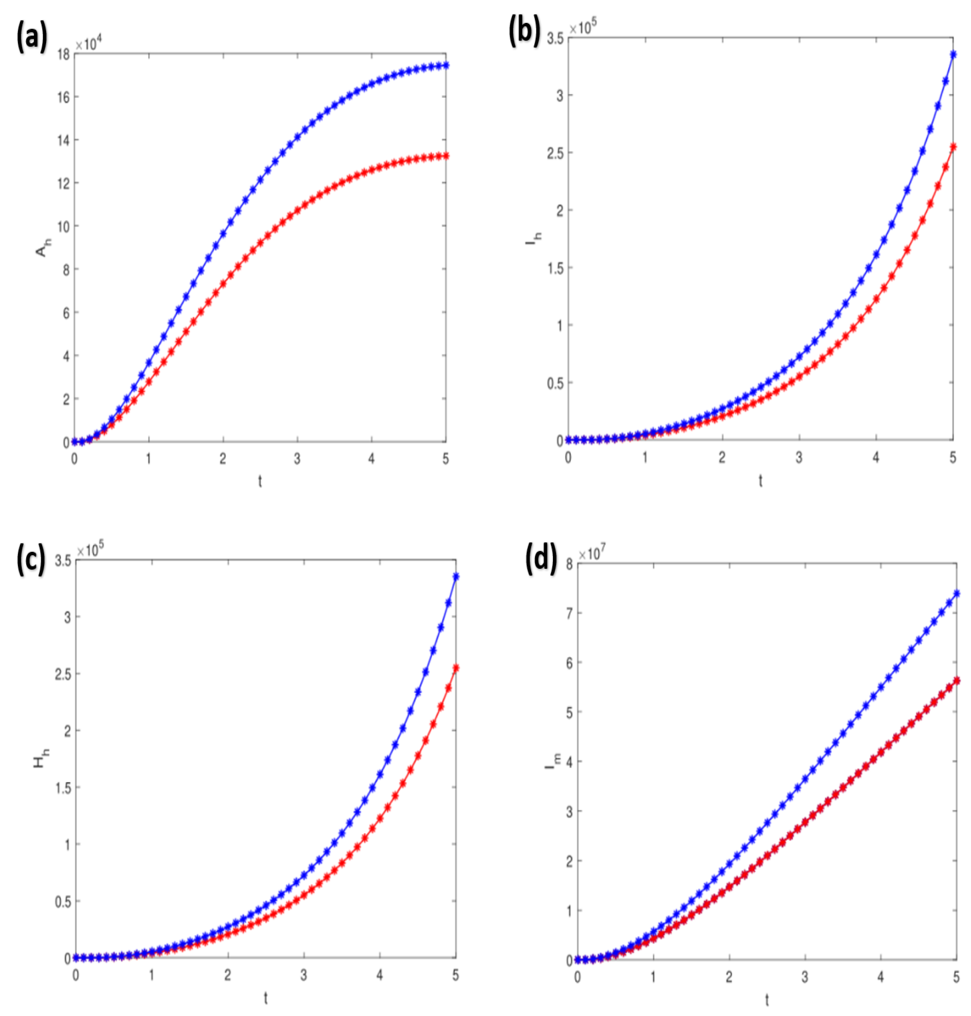
4.2. Numerical Simulations of the Dynamic Model

This section presents numerical simulations of the proposed YF model, utilizing the best-fit parameters derived earlier. The simulations were conducted using the classical Euler numerical method, a well-established technique widely applied in computational epidemiology research [46,47].
Figure 6a–j illustrates the dynamic behavior of individual compartments within the model’s state variables, based on the parameter values provided in Table 3 and Table 4. The results demonstrate the temporal evolution of each compartment as the outbreak progresses, providing insights into the epidemic’s progression.
Additionally, simulations were performed to analyze the dynamic behavior of various infected compartments under different values of key parameters, including σ h , θ , α h , and σ m . These parameters critically influence the transmission dynamics and the efficacy of control strategies within the model. The results, depicted in Figure 7a–d, highlight the sensitivity of the model outcomes to these parameters, offering valuable insights for designing effective intervention strategies.

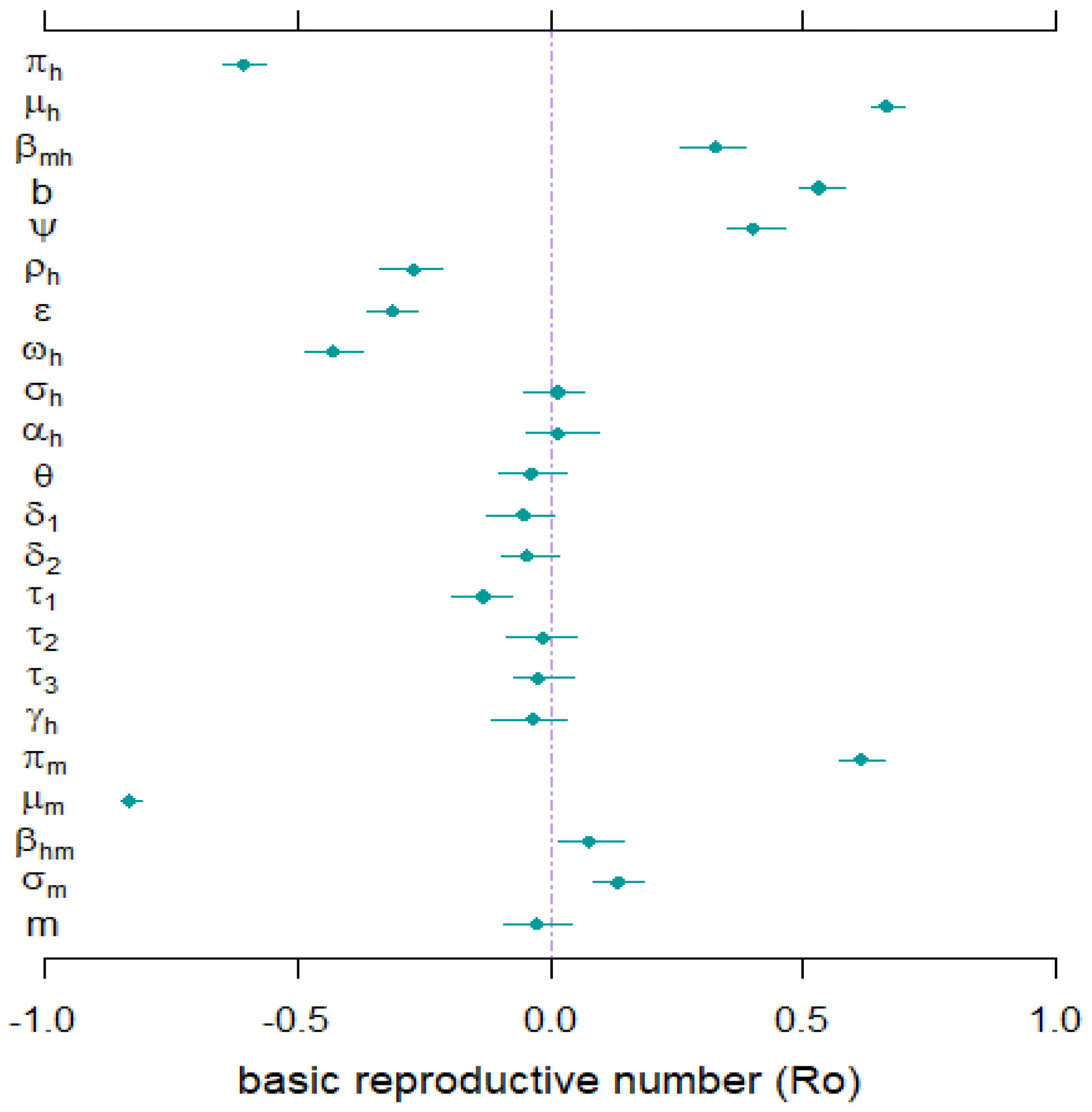
4.3. Sensitivity Analysis

In line with established methodologies [48,49,50], we conducted a sensitivity analysis using the Partial Ranked Correlation Coefficient (PRCC) approach. This analysis aimed to identify the most influential biological parameters within our model, specifically focusing on their impact on the Basic Reproduction Number ( R 0 ) and the Infection Attack Rate (IAR) as key indicators of disease spread dynamics, as outlined in Equation (1). The results of the sensitivity analysis, presented in Figure 8, highlighted the significant role of parameters such as μ m , π h , μ h , and π m in shaping the transmission dynamics of YF in Nigeria and potentially in similar epidemiological contexts.

5. Discussion and Conclusions

Mosquito-borne diseases (MBDs) are one of the major causes of mortality worldwide. MBDs are infections that are caused by the bite of an infected vector mosquito. MBDs can cause viruses such as chikungunya, dengue, malaria, YF, and Zika. Aedes or Haemagogus mosquitoes spread the YF virus, an arbovirus that belongs to the genus Flavivirus. Different mosquito species inhabit diverse habitats; some reproduce in home environments, some in the forest (jungle), and others in both (semi-domestic). YF, a life-threatening virus, is endemic in tropical and subtropical parts of Africa, Central America, and South America [1,2,3,4]. Controlling YF transmission, especially in poor resource settings where environmental hygiene/sanitation is not maintained properly, is challenging, although necessary. As mosquitoes usually breed in a dirty environment (in domestic or jungle areas), there is a need to maintain environmental hygiene at all times. This involves the relevant authorities providing adequate equipment to support ecological hygiene within the domestic habitats.
Mathematical modeling has historically been one of the most effective tools for combating disease transmission [18,51,52,53]. To aid in mitigating the transmission of YF outbreaks in endemic nations, we developed an explainable epidemiological model that incorporates active case detection and early hospitalization to prevent the spread of YF outbreaks. Theoretical analysis revealed that the model (1) has unique DGE, which is locally asymptotically stable when R 0 < 1 and unstable when R 0 > 1 . The epidemiological implication of the result above is that a small influx of YF infection will not cause a severe outbreak when R 0 < 1 . It is imperative to know that, for the model (1), the requirement for making R 0 < 1 is only adequate but not mandatory for YF containment. Therefore, control of a YF outbreak can be achieved with time when the R 0 can be drawn to a value < 1 and would strive when R 0 > 1 [29]. This is because allowing the recruitment of susceptible humans without carefully considering suitable control measures can make it even easier for the disease to spread more rapidly in a community, thereby causing severe epidemics. Furthermore, through sensitivity analysis results (see Section 4.3), we found that the parameters μ m and π h have a negative effect on R 0 , while the parameters μ h and π m have positive impacts on R 0 . These main factors should be highlighted for YF mitigation in Nigeria and elsewhere. The result also suggests that mosquito bites should be prevented, such as through environmental sanitation. Further analysis of the model (1) showed the existence of EE, a point in a community where the disease spreads and persists. The GAS of the EE has been investigated and it was found that the EE is GAS in Ω whenever R 0 > 1 under certain conditions (see Theorem 2), and unstable otherwise.
In an effort to restrict YF transmission in Nigeria and abroad, we also studied the effect of active case detection and early hospitalization techniques using optimal control theory. Thus, we incorporated two time-dependent control variables indicating ACD and early hospitalization into the model (1). We discovered that the overall number of asymptotically infected individuals and the population of hospitalized/isolated YF-infected humans can be reduced in the community by implementing time-dependent controls. Figure A1 and Figure A2 depict optimal control scenarios of the model with and without control, respectively. Our results align with the results obtained in [4,18,23], suggesting that the ACD strategy could be a promising tool for combating vector-borne disease in a community.
In our revised description of the optimal control analysis, described in Section 3.4, we underline the fundamental biological objectives of our research. The use of optimal control theory in YF transmission dynamics not only provides valuable insights into efficient intervention tactics but also fits within the larger framework of bioprocessing optimization. Our model shows how carefully manipulating parameters like vaccination and treatment rates can improve public health outcomes and reduce the effect of YF outbreaks. We have also contextualized our findings within the current literature on bioprocessing optimization, citing a broader variety of publications that demonstrate the importance of optimum control systems in the management of infectious diseases. This broader context highlights the importance of our research and its potential contributions to both theoretical and practical elements of disease control [51,52,53].
Epidemic models rely heavily on parameter fitting since it allows for the calibration of critical parameters based on real-world data, leading to more precise forecasts and better decisions. Essential parameters for understanding the dynamics of an epidemic can be estimated by fitting the model to observable data, including transmission rates, recovery rates, and beginning circumstances. Effective control tactics and public health interventions for infectious disease outbreaks can be greatly aided by the insights gained from properly fitting the model’s parameters. System 1 is calibrated well (see Figure 2) using monthly data of YF cases obtained from the Nigeria Centre for Disease Control and Prevention for January to December 2021 [24]. This is to ensure the validity of the outputs of the epidemic model with respect to reasonable biological parameters and to understand the YF epidemic trends in Nigeria.
Additionally, we simulated the model (1) to further investigate the general epidemiological behavior of each class, considering several critical model parameters. According to the outcomes of our simulation results, a few crucial parameters substantially affect the infectivity and transmissibility of the YF infection. These biological quantities can also help provide insight into the best ways to decrease YF transmission, such as by lowering the risks associated with the susceptible population and the number of infected people and halting the spread of infection among those who have already contracted the disease. In order to achieve this, the compartments’ dynamic features have been represented in Figure 6a–j. The influence of the parameter σ h on the class A h is shown in Figure 7a for different values, whereas Figure 7b shows the effect of the parameter θ on the class I h . Figure 7c shows how the parameter α h affects the class H h , whereas Figure 7d shows how the parameter σ affects the class I m . The numerical method employed in this study offers several advantages, including accuracy and efficiency in solving the differential equations governing YF transmission dynamics. Its suitability for handling the specific structure of our model enables robust simulations of the disease’s behavior [54,55,56]. However, we acknowledge certain limitations, such as its sensitivity to step size and potential challenges in accurately capturing non-linear dynamics, which may influence the model’s predictive capabilities.
In future studies, we intend to extend System (1) to incorporate seasonality, thereby uncovering additional dynamic features of YF transmission influenced by weather and climate conditions. This enhancement will enable us to better understand the effects of seasonal variations on vector populations, particularly mosquitoes, when sufficient seasonal data become available. By integrating these factors into our model, we aim to provide deeper insights into the epidemiology of YF and improve the effectiveness of control strategies. In conclusion, our study contributes significantly to understanding YF epidemiology and control strategies. Future research should focus on exploring the impact of seasonal variations, climate change, and vaccination strategies on YF dynamics. While our model captures essential aspects of YF transmission, it has limitations, such as simplifications in transmission dynamics and assumptions about population behaviors. Addressing these limitations and refining the model with more nuanced data and insights can further enhance its predictive power and relevance in guiding public health interventions [24]. Our study significantly enhances the understanding of YF transmission dynamics and the effectiveness of control measures. By elucidating the interplay between various factors influencing the spread of the disease, we provide valuable insights that can inform public health strategies aimed at mitigating the impact of YF outbreaks. Furthermore, our findings contribute to the current state of research in the field, emphasizing the implications for future research directions and public health initiatives. This integration of our model’s insights into existing strategies is crucial for developing effective responses to YF outbreaks.

Author Contributions

Conceptualization, N.L.A., M.M.A.-S., I.A. and S.S.M.; methodology, N.L.A., M.M.A.-S., I.A. and S.S.M.; software, S.S.M. validation, N.L.A., M.M.A.-S., I.A. and S.S.M.; formal analysis, N.L.A., M.M.A.-S., I.A. and S.S.M.; investigation, N.L.A., M.M.A.-S., I.A. and S.S.M.; resources, S.S.M.; data curation, S.S.M.; writing—original draft preparation, N.L.A., M.M.A.-S., I.A. and S.S.M.; writing—review and editing, N.L.A., M.M.A.-S., I.A. and S.S.M.; visualization, S.S.M.; supervision, M.M.A.-S. and S.S.M.; project administration, M.M.A.-S. and S.S.M.; funding acquisition, N.L.A. and M.M.A.-S. All authors have read and agreed to the published version of the manuscript.

Funding

This research was funded by the Deanship of Scientific Research (DSR) at Northern Border University, Arar, KSA “through the project number” NBU-FPEJ-2024-2089-02.

Data Availability Statement

All data were obtained from public domain (Nigeria Centre for Disease Control and Prevention via https://www.ncdc.gov.ng/) (accessed on 6 September 2022).

Acknowledgments

The authors extend their appreciation to the handling editor and unanimous reviwers for theie helpful comments. The authors extend their appreciation to the Deanship of Scientific Research (DSR) at Northern Border University, Arar, KSA, for funding this research work “through the project number” NBU-FPEJ-2024-2089-02.

Conflicts of Interest

The authors declare no conflict of interest.

Appendix A. Coefficient of the Polynomial (7)

The coefficients of the polynomial equation given in (10) are simplified as follows
a 4 = ( ( ( ω h ( q 8 + τ 2 ) q 2 + q 0 ( q 4 + q 3 ) ( q 8 + τ 1 ) ) σ h + q 8 q 2 ( q 4 + q 3 ) ) q 5 + ω h σ h q 2 q 3 ( q 8 + τ 3 ) ) q 7 2 q 6 μ m π h ( ( ( ( ( b β hm + μ m ) q 8 + μ m τ 2 ) ω h q 2 + ( ( b ψ β hm + μ m ) q 8 + μ m τ 1 ) q 0 ( q 4 + q 3 ) ) σ h + q 8 μ m q 2 ( q 4 + q 3 ) ) q 5 + μ m ω h σ h q 2 q 3 ( q 8 + τ 3 ) ) ,
a 3 = ( ( ( ω h ( q 8 + τ 2 ) q 2 + q 0 ( q 4 + q 3 ) ( q 8 + τ 1 ) ) ( q 7 ρ h + μ h ) σ h + ( ( ρ h + q 1 ) q 7 + μ h ) q 2 q 8 ( q 4 + q 3 ) ) q 5 + ω h σ h q 2 q 3 ( q 8 + τ 3 ) ( q 7 ρ h + μ h ) ) q 6 μ m π h q 7 ( ( ( ( ( b β hm μ m ) q 8 + μ m τ 2 ) ω h q 2 + ( ( b ψ β hm + μ m ) q 8 + μ m τ 1 ) q 0 ( q 4 + q 3 ) ) σ h + q 8 μ m q 2 ( q 4 + q 3 ) ) q 5 + μ m ω h σ h q 2 q 3 ( q 8 + τ 3 ) ) + ( ( ( ω h ( q 8 + τ 2 ) q 2 + q 0 ( q 4 + q 3 ) ( q 8 + τ 1 ) ) σ h + q 8 q 2 ( q 4 + q 3 ) ) q 5 + ω h σ h q 2 q 3 ( q 8 + τ 3 ) ) q 7 q 6 μ m π h ( ( ( ( ( b β hm + μ m ) q 8 + μ m τ 2 ) ω h q 2 + ( ( b ψ β hm + μ m ) q 8 + μ m τ 1 ) q 0 ( q 4 + q 3 ) ) ( q 7 ρ h + μ h ) σ h + ( ( ρ h + q 1 ) q 7 + μ h ) q 2 q 8 μ m ( q 4 + q 3 ) ) q 5 + μ m ω h σ h q 2 q 3 ( q 8 + τ 3 ) ( q 7 ρ h + μ h ) ) β hm q 8 π m σ h ( ω h q 2 + ψ q 0 ( q 4 + q 3 ) ) β mh ( ( γ h τ 2 ω h q 2 + τ 1 q 0 ( q 4 + q 3 ) ) σ h + q 8 q 1 q 2 ( q 4 + q 3 ) ) q 5 τ 3 γ h ω h σ h q 2 q 3 ) q 7 2 σ m q 5 b 2 ,
a 2 = q 8 q 1 q 2 q 5 ( q 4 + q 3 ) ( μ h + ρ h ) q 6 μ m π h q 7 ( ( ( ( ( b β hm + μ m ) q 8 + μ m τ 2 ) ω h q 2 + ( ( b ψ β hm + μ m ) q 8 + μ m τ 1 ) q 0 ( q 4 + q 3 ) ) σ h + q 8 μ m q 2 ( q 4 + q 3 ) ) q 5 + μ m ω h σ h q 2 q 3 ( q 8 + τ 3 ) ) + ( ( ( ω h ( q 8 + τ 2 ) q 2 + q 0 ( q 4 + q 3 ) ( q 8 + τ 1 ) ) ( q 7 ρ h + μ h ) σ h + ( ( ρ h + q 1 ) q 7 + μ h ) q 2 q 8 ( q 4 + q 3 ) ) q 5 + ω h σ h q 2 q 3 ( q 8 + τ 3 ) ( q 7 ρ h + μ h ) ) q 6 μ m π h ( ( ( ( ( b β hm + μ m ) q 8 + μ m τ 2 ) ω h q 2 + ( ( b ψ β hm + μ m ) q 8 + μ m τ 1 ) q 0 ( q 4 + q 3 ) ) ( q 7 ρ h + μ h ) σ h + ( ( ρ h + q 1 ) q 7 + μ h ) q 2 q 8 μ m ( q 4 + q 3 ) ) q 5 + μ m ω h σ h q 2 q 3 ( q 8 + τ 3 ) ( q 7 ρ h + μ h ) ) + ( ( ( ω h ( q 8 + τ 2 ) q 2 + q 0 ( q 4 + q 3 ) ( q 8 + τ 1 ) ) σ h + q 8 q 2 ( q 4 + q 3 ) ) q 5 + ω h σ h q 2 q 3 ( q 8 + τ 3 ) ) q 7 q 6 μ m 2 π h q 8 q 1 q 2 q 5 ( q 4 + q 3 ) ( μ h + ρ h ) + 2 q 7 σ m σ h β hm π m q 5 ( ω h q 2 + ψ q 0 ( q 4 + q 3 ) ) q 8 b 2 ( ( q 7 ρ h + μ h ) ( q 2 ( q 3 τ 3 + q 5 τ 2 ) ω h + q 0 q 5 τ 1 ( q 4 + q 3 ) ) γ h σ h 1 / 2 q 1 q 2 q 5 q 8 ( q 7 q 9 + q 7 ρ h + 2 μ h ) ( q 4 + q 3 ) ) β mh ,
a 1 = q 8 q 1 q 2 q 5 ( q 4 + q 3 ) ( μ h + ρ h ) q 6 μ m π h ( ( ( ( ( b β hm + μ m ) q 8 + μ m τ 2 ) ω h q 2 + ( ( b ψ β hm + μ m ) q 8 + μ m τ 1 ) q 0 ( q 4 + q 3 ) ) ( q 7 ρ h + μ h ) σ h + ( ( ρ h + q 1 ) q 7 + μ h ) q 2 q 8 μ m ( q 4 + q 3 ) ) q 5 + μ m ω h σ h q 2 q 3 ( q 8 + τ 3 ) ( q 7 ρ h + μ h ) ) + ( ( ( ω h ( q 8 + τ 2 ) q 2 + q 0 ( q 4 + q 3 ) ( q 8 + τ 1 ) ) ( q 7 ρ h + μ h ) σ h + ( ( ρ h + q 1 ) q 7 + μ h ) q 2 q 8 ( q 4 + q 3 ) ) q 5 + ω h σ h q 2 q 3 ( q 8 + τ 3 ) ( q 7 ρ h + μ h ) ) q 6 μ m 2 π h q 8 q 1 q 2 q 5 ( q 4 + q 3 ) ( μ h + ρ h ) ( β hm q 8 2 π m σ h ( ω h q 2 + ψ q 0 ( q 4 + q 3 ) ) β mh q 9 μ h q 1 q 2 q 5 ( q 4 + q 3 ) q 7 + β hm q 8 π m σ h ( ω h q 2 + ψ q 0 ( q 4 + q 3 ) ) β mh ( ( γ h ( τ 2 ω h q 2 + τ 1 q 0 ( q 4 + q 3 ) ) ( q 7 ρ h + μ h ) σ h + q 8 q 1 q 2 ( q 4 + q 3 ) ( q 7 q 9 + μ h ) ) q 5 τ 3 γ h ω h σ h q 2 q 3 ( q 7 ρ h + μ h ) ) ( q 7 ρ h + μ h ) ) σ m q 5 b 2 ,
a 0 = β hm π m σ h ( ω h q 2 + ψ q 0 ( q 4 + q 3 ) ) β mh q 9 μ h ( q 7 ρ h + μ h ) σ m b 2 q 1 q 2 ( q 4 + q 3 ) ( μ h + ρ h ) 2 q 6 μ m 2 π h = ( 1 R 0 2 ) .

Appendix B. Summary Tables of the Number of Possible Positive Real Roots of Equation (7)

The Descartes’ rule of sign changes was employed on Equation (7) to obtain 32 various possibilities for the positive real roots of the polynomial (10) given in Table A1 below [23,33].
Table A1. Number of possible positive real roots of Equation (7).
Case C 4 C 3 C 2 C 1 C 0 R 0 No. of Sign ChangesPossible + Real Roots
1+++++ R 0 < 1 00
2++++ R 0 > 1 11
3+ R 0 > 1 11
4++ R 0 > 1 11
5+++ R 0 > 1 11
6++ R 0 < 1 20, 2
7+++ R 0 < 1 20, 2
8+++ R 0 < 1 20, 2
9++++ R 0 < 1 20, 2
10++++ R 0 < 1 20, 2
11++++ R 0 < 1 20, 2
12++ R 0 > 1 31, 3
13++ R 0 > 1 31, 3
14+++ R 0 > 1 31, 3
15+++ R 0 > 1 31, 3
16+++ R 0 < 1 40, 2, 4
17 R 0 > 1 00
18++++ R 0 < 1 11
19+ R 0 < 1 11
20++ R 0 < 1 11
21++ R 0 < 1 11
22+++ R 0 < 1 11
23+++ R 0 > 1 20, 2
24+ R 0 > 1 20, 2
25+ R 0 > 1 20, 2
26+ R 0 > 1 20, 2
27++ R 0 > 1 20, 2
28++ R 0 > 1 20, 2
29++ R 0 < 1 31, 3
29+++ R 0 < 1 31, 3
31+++ R 0 < 1 31, 3
32++ R 0 > 1 40, 2, 4

Appendix C. The Proof of Theorem 2

Proof. 
Define a Lyapunov function as follows
L ( t ) = n 1 ( S h S h * S h * ln S h S h * ) + n 2 ( V h V h * V h * ln V h V h * ) + n 3 ( E h E h * E h * ln E h E h * ) + n 4 ( A h A h * A h * ln A h A h * ) + n 5 ( I h I h * I h * ln I h I h * ) + n 6 ( H h H h * H h * ln H h H h * ) + n 7 ( S m S m * S m * ln S m S m * ) + n 8 ( E m E m * E m * ln E m E m * ) + n 9 ( I m I m * I m * ln I m I m * ) ,
where n 1 = n 2 = n 3 = 1 , n 4 = λ h * S H * q 0 σ h E h * , n 5 = q 7 λ h * V h * ( θ ) , n 6 = 1 q 3 I h * , n 7 = n 8 = 1 , and n 9 = λ m * S m * σ m E m * .
Thus, the Lyapunov derivative computed along solutions of the system (1) is given by
L ˙ ( t ) = n 1 ( 1 S h * S h ) S h ˙ + n 2 ( 1 V h * V h ) V h ˙ n 3 ( 1 E h * E h ) E h ˙ + + n 4 ( 1 A h * A h ) A h ˙ + n 5 ( 1 I h * I h ) I h ˙ + n 6 ( 1 H h * H h ) H h ˙ + n 7 ( 1 S m * S m ) S m ˙ + n 8 ( 1 E m * E m ) E m ˙ + n 9 ( 1 I m * I m ) I m ˙ .
Hence, simplifying each term of (A2), we have
n 1 1 S h * S h S h ˙ = n 1 1 S h * S h π h + γ h R h λ h S h q 9 S h = n 1 1 S h * S h λ h * S h * + q 9 S h * λ h S h q 9 S h = n 1 λ h * S h * 1 S h * S h 1 λ h S h λ h * S h * + n 1 q 9 1 S h * S h ( S h * S h ) n 1 λ h * S h * 1 S h * S h 1 λ h S h * λ h * S h * n 1 q 9 ( S h S h * ) 2 S h n 1 λ h * S h * 1 λ h S h λ h * S h * S h * S h + λ h λ h * ,
Similarly,
n 2 1 V h * V h V h ˙ n 2 q 7 λ h * V h * 1 λ h V h λ h * V h * V h * V h + λ h λ h * .
Moreover,
n 3 1 E * E h λ h S h + q 7 λ h V h ( λ h * S h * + q 7 λ h * V h * ) E h E h * = n 3 1 E * E h ( λ h S h λ h * S h * E h E h * ) + ( q 7 λ h V h q 7 λ h * V h * E h E h * ) = n 3 λ h * S h * 1 E * E h λ h S h λ h * S h * E h E h * + n 3 q 7 λ h * V h * 1 E * E h λ h V h λ h * V h * E h E h * = n 3 λ h * S h * λ h S h λ h * S h * E h E h * λ h S h E h * λ h * S h * E h + 1 + n 3 q 7 λ h * V h * λ h V h λ h * V h * E h E h * λ h V h E h * λ h * V h * E h + 1 ,
Similarly,
n 4 1 A h * A h A h ˙ = n 4 q 0 σ h E h * E h E h * A h A h * A h * E h A h E h * + 1 ,
n 5 1 I h * I h I h ˙ = n 5 ω h σ h E h * E h E h * I h I h * I h * E h I h E h * + 1 ,
and
n 6 1 H h * H h H h ˙ = n 6 q 3 I h * I h I h * H h H h * H h * I h H h I h * + 1 .
Moreover,
n 7 1 S m * S m S m ˙ n 7 λ m * S m * 1 λ m S m λ m * S m * S m * S m + λ m λ m * ,
and
n 8 1 E m * E m E m ˙ = n 8 λ m * S m * λ m S m λ m * S m * E m E m * E m * λ m S m E m λ m * S m * + 1 .
Additionally,
n 9 1 I m * I m I m ˙ = n 9 σ m E m * E m E m * I m I m * I m * E m I m E m * + 1 .
Thus, the Lyapunov derivative is now given by
L ˙ ( t ) n 1 λ h * S h * [ 1 λ h S h λ h * S h * S h * S h + λ h λ h * ] + n 2 q 7 λ h * V h * [ 1 λ h V h λ h * V h * V h * V h + λ h λ h * ] + n 3 λ h * S h * [ λ h S h λ h * S h * E h E h * E h * λ h S h E h λ h * S h * + 1 ] + n 3 q 7 λ h * V h * [ λ h V h λ h * S h * E h E h * E h * λ h V h E h λ h * V h * + 1 ] + n 4 q 0 σ h E h * [ E h E h * A h A h * A h * E h A h E h * + 1 ] + n 5 ω h σ h E h * [ E h E h * I h I h * I h * E h I h E h * + 1 ] + n 6 q 3 I h * [ I h I h * H h H h * H h * I h H h I h * + 1 ] + n 7 λ m * S m * [ 1 λ m S m λ m * S m * S m * S m + λ m λ m * ] + n 8 λ m * S m * [ λ m S m λ m * S m * E m E m * E m * λ m S m E m λ m * S m * + 1 ] + n 9 σ m E m * [ E m E m * I m I m * I m * E m I m E m * + 1 ] .
According to previous studies [31,36], suppose a function be defined by v ( x ) = 1 x + ln x . If x > 0 , then v ( x ) 0 , and if x = 1 , we have v ( x ) = 0 . Thus, x 1 ln ( x ) for any x > 0 . Thus, after substituting n i ( i = 1 9 ) and simplifying each term in Equation (A12), we have
L ˙ ( t ) λ h * S h * 2 S h * S h E h E h * λ h S h E h * λ h * S h * E h + λ h λ h * + q 7 λ h * V h * 2 V h * V h E h E h * λ h V h E * λ h * V h * E h + λ h λ h * + λ h * S h * E h E h * l n E h E h * + l n A h A * A h A h * + q 7 λ h * V h * E h E h * l n E h E h * + l n I h I h * I h I h * + I h I h * l n I h I h * + l n H h H h * H h H h * + λ m * S m * 2 S m * S m E m E m * λ m S m E m * λ m * S m * E h + λ m λ m * + λ m * S m * E m E m * l n E m E m * + l n I m I m * I m I m * .
where
λ h * S h * [ 2 S h * S h E h E h * λ h S h E h * λ h * S h * E h + λ h λ h * ] = λ h * S h * ( 1 λ h λ h * ) ( 1 A h λ h * A h * λ h ) + 3 S h * S h λ h S h E h * λ h * S h * E h A h λ * A h * λ h E h E h * + A h A h * λ h * S h * ( S h * S h 1 ) ( λ h S h E h * λ h * S h * E h 1 ) ( A h λ h * A h * λ h 1 ) E h E h * + A h A h * λ h * S h * ln ( S h * S h λ h S h E h * λ * S h * E h A h λ h * A h * λ h ) E h E h * + A h A h * = λ h * S h * [ A h A h * ln ( A h A h * ) + ln ( E h E h * ) E h E h * ] .
Similarly,
q 7 λ h * V h * [ 2 V h * V h E h E h * λ h V h E h * λ h * V h * E h + λ h λ h * ] q 7 λ h * V h * [ I h I h * ln ( I h I h * ) + ln ( E h E h * ) E h E h * ] ,
and
λ m * S m * [ 2 S m * S m E m E m * λ m S m E m * λ m * S m * E m + λ m λ m * ] λ m * S m * [ I m I m * ln ( I m I m * ) + ln ( E m E m * ) E m E m * ] .
Therefore, combining the above computations together with condition (11) ensures that d L dt 0 . Furthermore, the strict inequality d L dt = 0 holds only for S h = S h * , V h = V h * , E h = E h * , A h = A h * , I h = I h * , H h = H h * , R h = R h * , S m = S m * E m = E m * , and I m = I m * . Thus, the endemic equilibrium state E * is the only positive invariant set to the system (1) contained entirely in ( S h , V h , E h , A h , I h , H h , R h , S m , E m , I m ) Ω : S h = S h * , V h = V h * , E h = E h * , A h = A h * , I h = I h * , H h = H h * , R h = R h * , S m = S m * , E m = E m * , I m = I m * . Thus, according to LaSalle’s invariance principle [57], every solution to the equations in (A2) with initial conditions in Ω converge to a stable endemic equilibrium point, E * , as t . Hence, the positive endemic equilibrium is GAS. □

Appendix D. Proof of Theorem 3

Proof. 
Considering the existence of the control functions, we employed Pontryagin’s Maximum Principle [37,38] to find the adjoint variables and the expressions of the control functions. Given that:
H = a 1 i h + a 2 H h + w 1 u 1 2 2 + w 2 u 2 2 2 + λ 1 π h + γ h R h b β mh I m S h N h * ρ h + μ h S h + λ 2 ρ h S h 1 ϵ b β mh I m V h N h * μ h V h + λ 3 b β mh I m S h + 1 ϵ V h N h * σ h + μ h E h + λ 4 1 ω h σ h E h τ 1 + μ h A h + λ 5 ω h σ h E h u 1 + u 2 i h δ 1 + τ 2 + μ h i h + λ 6 u 1 + u 2 i h δ 2 + τ 3 + μ h H h + λ 7 τ 1 A h + τ 2 i h + τ 3 H h γ h + μ h R h + λ 8 S m b β hm ψ A h + I h N h * μ m S m + π m + λ 9 S m b β hm ψ A h + I h N h * σ m + μ m E m + λ 10 E m σ m i m μ m
so that d λ i dt = H i , and the transversality conditions λ i ( t f ) = 0 , where i = S h , V h I m , thus, the adjoint system is given as follows:
d λ 1 dt = H S h , λ 1 ( t f ) = 0 , d λ 2 dt = H V h , λ 2 ( t f ) = 0 , d λ 3 dt = H E h , λ 3 ( t f ) = 0 , d λ 4 dt = H A h , λ 4 ( t f ) = 0 , d λ 5 dt = H I h , λ 5 ( t f ) = 0 , d λ 6 dt = H H h , λ 6 ( t f ) = 0 , d λ 7 dt = H R h , λ 7 ( t f ) = 0 , d λ 8 dt = H S m , λ 8 ( t f ) = 0 , d λ 9 dt = H E m , λ 9 ( t f ) = 0 , d λ 10 dt = H I m , λ 10 ( t f ) = 0 .
Therefore, the adjoint system given above is evaluated at the optimal control’s corresponding state variables, resulting in the stated adjoint system in the theorem, and is thus given by:
d λ 1 dt = λ 1 b β m h I m * N h * + b β m h I m * S h * N h * 2 ρ h μ h + λ 2 ρ h + 1 ϵ b β m h I m * V h * N h * 2 + λ 3 b β m h I m * N h * b β m h I m * S h * + 1 ϵ V h * N h * 2 + λ 8 S m * b β m h ψ A h * + I h * N h * 2 λ 9 S m * b β m h ψ A h * + I h * N h * 2 , d λ 2 dt = λ 1 b β m h I m * S h * N h * 2 + λ 2 1 ϵ b β m h I m * N h * + 1 ϵ b β m h I m * V h * N h * 2 μ h + λ 3 1 ϵ b β m h I m * N h * b β m h I m * S h * + 1 ϵ V h * N h * 2 + λ 8 S m * b β m h ψ A h + I h N h * 2 λ 9 S m * b β m h ψ A h * + I h * N h * 2 , d λ 3 dt = λ 1 b β m h I m * S h * N h * 2 + λ 2 1 ϵ b β m h I m * V h * N h * 2 + λ 3 b β m h I m * S h + 1 ϵ V h * N h * 2 σ h μ h + λ 4 1 ω h σ h + λ 5 ω h σ h + λ 8 S m * b β m h ψ A h * + I h * N h * 2 λ 9 S m * b β m h ψ A h * + I h * N h * 2 ,
d λ 4 dt = λ 1 b β m h I m * S h * N h * 2 + λ 2 1 ϵ b β m h I m * V h * N h * 2 λ 3 b β m h I m * S h * + 1 ϵ V h * N h * 2 + λ 4 τ 1 μ h + λ 7 τ 1 + λ 8 S m * b β m h ψ N h * + S m * b β m h ψ A h * + I h N h * 2 + λ 9 S m * b β m h ψ N h * S m * b β m h ψ A h * + I h * N h * 2 , d λ 5 dt = a 1 + λ 1 b β m h I m S h * N h * 2 + λ 2 1 ϵ b β m h I m * V h * N h * 2 λ 3 b β m h I m * S h * + 1 ϵ V h * N h * 2 + λ 5 u 1 u 2 δ 1 τ 2 μ h + λ 6 u 1 + u 2 + λ 7 τ 2 + λ 8 S m * b β m h N h * + S m * b β m h ψ A h * + I h * N h * 2 + λ 9 S m * b β m h N h * S m * b β m h ψ A h * + I h * N h * 2 , d λ 6 dt = a 2 + λ 1 b β m h I m * S h * N h * 2 + λ 2 1 ϵ b β m h I m * V h * N h * 2 λ 3 b β m h I m * S h * + 1 ϵ V h * N h * 2 + λ 6 δ 2 τ 3 μ h + λ 7 τ 3 + λ 8 S m * b β m h ψ A h * + I h * N h * 2 λ 9 S m * b β m h ψ A h + I h * N h * 2 , d λ 7 dt = λ 1 γ h + b β m h I m * S h * N h * 2 + λ 2 1 ϵ b β m h I m * V h * N h * 2 λ 3 b β m h I m * S h * + 1 ϵ V h * N h * 2 + λ 7 γ h μ h + λ 8 S m * b β m h ψ A h * + I h * N h * 2 λ 9 S m * b β m h ψ A h * + I h * N h * 2 , d λ 8 dt = λ 8 b β m h ψ A h * + I h * N h * μ m + λ 9 b β m h ψ A h * + I h * N h * , d λ 9 dt = λ 9 σ m μ m + λ 10 σ m , d λ 10 dt = λ 1 b β m h S h * N h * λ 2 1 ϵ b β m h V h * N h * + λ 3 b β m h S h * + 1 ϵ V h * N h * λ 10 μ m .
Differentiating the Hamiltonian function with regard to control variables in the interior of the control set and solving for controls ( u 1 * , u 2 * ) yields optimality requirements as follows: Given the representations of the control functions H u i = 0 at u i = u i * for i = 1 , 2 , . 10 , and following the standard optimality arguments, we have
u 1 * = min max ( λ 5 * λ 6 * ) I h * w 1 , 0 , 1 u 2 * = min max ( λ 5 * λ 6 * ) I h * w 2 , 0 , 1 .
Hence, having determined the representations of the control functions u 1 * , u 2 * and the adjoint equations with their transversality conditions, we ensured the existence of the optimal levels needed to minimize the spread of YF infection.

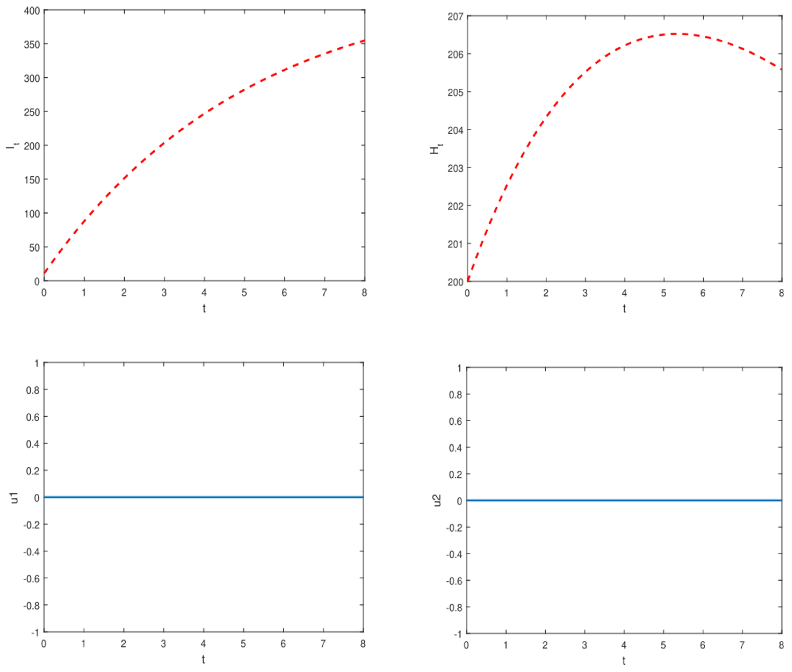
Appendix E. Numerical Illustration of the Optimal Control Problems

This subsection presents the numerical results of employing optimal control methods for managing YF transmission dynamics in Nigeria. We utilized two control functions, u 1 ( t ) representing active case detection and u 2 ( t ) representing early hospitalization, to optimize YF control and prevention strategies. The comparison between scenarios with control ( u 1 ( t ) 0 and u 2 ( t ) 0 ) and without control ( u 1 ( t ) = 0 and u 2 ( t ) = 0 ) revealed significant differences in the state variables. Detailed results are depicted in Figure A1 and Figure A2, while Table 4 provides the parameter values utilized in the optimal control simulations.
Figure A1. Simulations of the model illustrate the dynamics of symptomatically infected individuals ( I h ) and hospitalized infected individuals ( H h ) in the absence of control measures.
Mathematics 12 03817 g0a1
Figure A2. Simulations of the model depicting the dynamics of symptomatically infected individuals ( I h ) and hospitalized infected individuals ( H h ) when optimal control measures are implemented.
Mathematics 12 03817 g0a2

Appendix F. Summary Tables for Parameter Estimates

Appendix F.1. Estimates of Comparison Between Number of Actual Symptomatically Infected Individuals and Predicted Ones

Table A2. Comparison between number of real symptomatically infected individuals and predicted ones with associated standard errors and the confidence intervals.
Real CasesPredictedStandard ErrorConfidence Interval
19.19.6.74915{3.43642, 34.5636}
23.33.71076.92959{17.7311, 49.6904}
51.46.41937.82933{28.3648, 64.4737}
51.55.2787.09286{38.9219, 71.6342}
54.61.56727.38555{44.5361, 78.5983}
61.66.05998.95316{45.4139, 86.706}
70.69.2967.95725{50.9465, 87.6454}
70.71.65187.96207{53.2912, 90.0124}
74.73.38978.38355{54.0572, 92.7223}
82.74.69248.30785{55.5345, 93.8503}
82.75.68677.5411{58.2969, 93.0765}
82.76.46078.12709{57.7196, 95.2018}

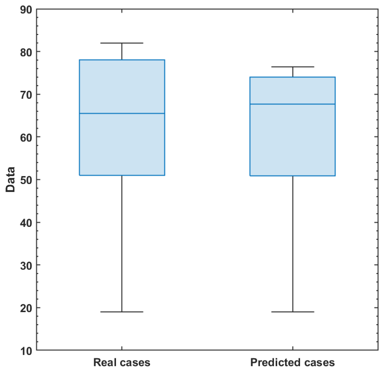
Appendix F.2. Summary Results for Actual and Predicted Data

Table A3. Summary statistics for the real data, and the predicted data obtained under simulations of the model (1) for the symptomatically infected individuals I h .
DataMin.1st Qu.MedianMean3rd Qu.Max.SD
Real cases1.90 × 10 1 5.10 × 10 1 6.55 × 10 1 5.99 × 10 1 7.80 × 10 1 8.20 × 10 1 2.15 × 10 1
Predicted1.90 × 10 1 5.08 × 10 1 6.77 × 10 1 6.03 × 10 1 7.40 × 10 1 7.65 × 10 1 1.85 × 10 1

References

  1. World Health Organization. Yellow Fever. WHO Fact Sheets. 2019. Available online: https://www.who.int/news-room/fact-sheets/detail/yellow-fever (accessed on 11 November 2019).
  2. Kung’Aro, M.; Luboobi, L.S.; Shahada, F. Modelling and stability analysis of SVEIRS yellow fever two-host model. Gulf J. Math. 2015, 3, 106–129. [Google Scholar] [CrossRef]
  3. Monath, T.P.; Vasconcelos, P.F.C. Yellow fever. J. Clinical Virol. 2015, 64, 160–173. [Google Scholar] [CrossRef]
  4. Zhao, S.; Stone, L.; Gao, D.; He, D. Modelling the large-scale yellow fever outbreak in Luanda, Angola, and the impact of vaccination. PLoS Negl. Trop. Dis. 2018, 12, e0006158. [Google Scholar] [CrossRef]
  5. World Health Organization. Yellow Fever-Nigeria. WHO Reports. Available online: https://www.who.int/emergencies/disease-outbreak-news/item/2020-DON299 (accessed on 11 November 2019).
  6. Duijzer, L.E.; van Jaasveld, W.; Dekker, R. Literature review: The vaccine supply chain. Eur. J. Oper. Res. 2018, 268, 174–192. [Google Scholar] [CrossRef]
  7. Robbins, M.J.; Lunday, B.J. A bilevel formulation of the pediatric vaccine pricing problem. Eur. J. Oper. Res. 2016, 248, 634–645. [Google Scholar] [CrossRef]
  8. Kraemer, M.U.; Faria, N.R.; Reiner, J.R.; Golding, N.; Nikolay, B.; Stasse, S.; Johansson, M.A.; Salje, H.; Faye, O.; Wint, G.W.; et al. Spread of yellow fever virus outbreak in Angola and the Democratic Republic of the Congo 2015–16: A modelling study. Lancet Infect. Dis. 2017, 17, 330–338. [Google Scholar] [CrossRef]
  9. Abdulrashid, I.; Tomas, C.; Xiaoying, H. Effects of delays in mathematical models of cancer chemotherapy. Pure Appl. Funct. Anal. 2022, 7, 1103–1126. [Google Scholar]
  10. Abdulrashid, I.; Han, X. A mathematical model of chemotherapy with variable infusion. Commun. Pure Appl. Anal. 2020, 19, 1875–1890. [Google Scholar] [CrossRef]
  11. Abdulrashid, I.; Alsammani, A.M.; Han, X. Stability analysis of a chemotherapy model with delays. Disc. Cont. Dyn. Syst.-B 2019, 24, 989–1005. [Google Scholar] [CrossRef]
  12. Abdulrashid, I.; Ghazzai, H.; Han, X.; Massoud, Y. Optimal Control Treatment Analysis for the Predator-Prey Chemotherapy Model. In Proceedings of the 2019 31st International Conference on Microelectronics (ICM), Cairo, Egypt, 15–18 December 2019; pp. 296–299. [Google Scholar]
  13. Al-Shomrani, M.M.; Musa, S.S.; Yusuf, A. Unfolding the transmission dynamics of monkeypox virus: An epidemiological modelling analysis. Mathematics 2023, 11, 1121. [Google Scholar] [CrossRef]
  14. Gu, Y.; Khan, M.; Zarin, R.; Khan, A.; Yusuf, A.; Humphries, U.W. Mathematical analysis of a new nonlinear dengue epidemic model via deterministic and fractional approach. Alexandria Eng. J. 2023, 67, 1–21. [Google Scholar] [CrossRef]
  15. Zarin, R.; Khan, M.; Khan, A.; Yusuf, A. Deterministic and fractional analysis of a newly developed dengue epidemic model. Waves Random Complex Media 2023, 1–34. [Google Scholar] [CrossRef]
  16. Adel, M.; Khader, M.M.; Ahmad, H.; Assiri, T.A. Approximate analytical solutions for the blood ethanol concentration system and predator-prey equations by using variational iteration method. AIMS Math. 2023, 8, 19083–19096. [Google Scholar] [CrossRef]
  17. Shearer, F.M.; Longbottom, J.; Browne, A.J.; Pigott, D.M.; Brady, O.J.; Kraemer, M.U.; Marinho, F.; Yactayo, S.; de Araújo, V.E.; da Nóbrega, A.A.; et al. Existing and potential infection risk zones of yellow fever worldwide: A modelling analysis. Lancet Glob. Health 2018, 6, e270–e278. [Google Scholar] [CrossRef]
  18. Teklu, S.W.; Rao, K.P. HIV/AIDS–Pneumonia Codynamics Model Analysis with Vaccination and Treatment. Comput. Math. Methods Med. 2022, 2022, 3105734. [Google Scholar] [CrossRef]
  19. Alshehri, A.; El Hajji, M. Mathematical study for Zika virus transmission with general incidence rate. AIMS Math. 2022, 7, 7117–7142. [Google Scholar] [CrossRef]
  20. Fraser, K.; Hamlet, A.; Jean, K.; Ramos, D.G.; Romano, A.; Horton, J.; Cibrelus, L.; Ferguson, N.; Gaythorpe, K.A. Assessing yellow fever outbreak potential and implications for vaccine strategy. medRxiv 2023. [Google Scholar] [CrossRef]
  21. Kung’aro, M. Mathematical Modelling of Intra and Inter Dynamics and Control of Yellow Fever in Primate and Human Populations. Ph.D. Thesis, The Nelson Mandela African Institution of Science and Technology, Arusha, Tanzania, 2016. [Google Scholar] [CrossRef]
  22. Caasi, J.A.; Joseph, B.M.; Kodiyamplakkal, H.J.; Manibusan, J.R.; Camacho Aquino, L.J.; Oh, H.; Rychtář, J.; Taylor, D. A game-theoretic model of voluntary yellow fever vaccination to prevent urban outbreaks. Games 2022, 13, 55. [Google Scholar] [CrossRef]
  23. Ghosh, I.; Tiwari, P.K.; Chattopadhyay, J. Effect of active case finding on dengue control: Implications from a mathematical model. J. Theoret. Biol. 2019, 464, 50–62. [Google Scholar] [CrossRef]
  24. Nigeria Centre for Disease Control and Prevention. Yellow Fever. Available online: https://www.ncdc.gov.ng/ncdc.gov.ng/diseases/sitreps/?cat=10&name=An%20update%20of%20Yellow%20Fever%20outbreak%20in%20Nigeria (accessed on 4 August 2022).
  25. Nigeria Centre for Disease Control. Disease Situation Report: An Update of Lassa Fever Outbreak in Nigeria. 2018. Available online: https://www.ncdc.gov.ng/ncdc.gov.ng/diseases/sitreps (accessed on 6 March 2022).
  26. World Health Organization. Yellow Fever. 2021. Available online: https://www.who.int/news-room/fact-sheets/detail/yellow-fever (accessed on 2 December 2021).
  27. Hussaini, N.; Lubuma, J.M.; Barley, K.; Gumel, A.B. Mathematical analysis of a model for AVL-HIV co-endemicity. Math. Biosci. 2016, 271, 80–95. [Google Scholar] [CrossRef]
  28. Diekmann, O.; Heesterbeek, J.; Metz, J. On the definition and the computation of the basic reproduction ratio R0 in models for infectious diseases in heterogeneous populations. J. Math. Biol. 1990, 28, 365–382. [Google Scholar] [CrossRef] [PubMed]
  29. van den Driessche, P.; Watmough, J. Reproduction numbers and sub-threshold endemic equilibria for compartmental models of disease transmission. Math. Biosci. 2002, 180, 29–48. [Google Scholar] [CrossRef] [PubMed]
  30. Chowell, G.; Viboud, C.; Simonsen, L.; Moghadas, S.M. Characterizing the reproduction number of epidemics with early subexponential growth dynamics. J. R. Soc. Interface 2016, 13, 0659. [Google Scholar] [CrossRef]
  31. Yang, C.; Wang, X.; Gao, D.; Wang, J. Impact of awareness programs on cholera dynamics: Two modeling approaches. Bull. Math. Biol. 2017, 79, 2109–2131. [Google Scholar] [CrossRef]
  32. Musa, S.S.; Zhao, S.; Hussaini, N.; Habib, A.G.; He, D. Mathematical modeling and analysis of meningococcal meningitis transmission dynamics. Int. J. Biomath. 2020, 13, 2050006. [Google Scholar] [CrossRef]
  33. Wang, X. A simple proof of Descartes’s rule of signs. Am. Math. Mon. 2004, 111, 525. [Google Scholar] [CrossRef]
  34. Molnar, S.; Szidarovsky, F. Some notes on the time-variant Lyapunov theory. Eur. J. Oper. Res. 1996, 89, 668–670. [Google Scholar] [CrossRef]
  35. Tadic, V. Stochastic gradient algorithm with random truncations. Eur. J. Oper. Res. 1997, 101, 261–284. [Google Scholar] [CrossRef]
  36. Sun, G.Q.; Xie, J.H.; Huang, S.H.; Jin, Z.; Li, M.T.; Liu, L. Transmission dynamics of cholera: Mathematical modeling and control strategies. Commun. Non. Sci. Numer. Simulat. 2017, 45, 235–244. [Google Scholar] [CrossRef]
  37. Farouk, T.S.; Evren, H. An optimal control approach for the interaction of immune checkpoints, immune system, and BCG in the treatment of superficial bladder cancer. Eur. Phys. J. Plus 2018, 133, 241. [Google Scholar]
  38. Kopp, R.E. Pontryagin maximum principle. In Mathematics in Science and Engineering; Elsevier: Amsterdam, The Netherlands, 1962; Volume 5, pp. 255–279. [Google Scholar]
  39. Garba, S.M.; Lubuma, J.M.; Tsanou, B. Modeling the transmission dynamics of the COVID-19 Pandemic in South Africa. Math. Biosci. 2020, 328, 108441. [Google Scholar] [CrossRef] [PubMed]
  40. Hussaini, N.; Okuneye, K.; Gumel, A.B. Mathematical analysis of a model for zoonotic visceral leishmaniasis. Infect. Dis. Model. 2017, 2, 455–474. [Google Scholar] [CrossRef] [PubMed]
  41. Musa, S.S.; Zhao, S.; Hussaini, N.; Usaini, S.; He, D. Dynamics analysis of typhoid fever with public health education programs and final epidemic size relation. Results Appl. Math. 2021, 10, 100153. [Google Scholar] [CrossRef]
  42. He, D.; Zhao, S.; Lin, Q.; Musa, S.S.; Stone, L. New estimates of the Zika virus epidemic attack rate in Northeastern Brazil from 2015 to 2016: A modelling analysis based on Guillain-Barré Syndrome (GBS) surveillance data. PLoS Negl. Trop. Dis. 2020, 14, e0007502. [Google Scholar] [CrossRef]
  43. Roop-O, P.; Chinviriya, W.; Chinviriyasit, S. The effect of incidence function in backward bifurcation for malaria model with temporary immunity. Math. Biosci. 2015, 265, 47–64. [Google Scholar] [CrossRef]
  44. Musa, S.S.; Zhao, S.; Chan, H.S.; Jin, Z.; He, D. A mathematical model to study the 2014–2015 large-scale dengue epidemics in Kaohsiung and Tainan cities in Taiwan, China. Math. Biosci. Eng. 2019, 16, 3841–3863. [Google Scholar] [CrossRef] [PubMed]
  45. Garba, S.M.; Gumel, A.B.; Bukar, M.R.A. Backward bifurcations in dengue transmission dynamics. Math. Biosci. 2008, 215, 11–25. [Google Scholar] [CrossRef] [PubMed]
  46. Musa, S.S.; Baba, I.A.; Yusuf, A.; Sulaiman, T.A.; Aliyu, A.I.; Zhao, S.; He, D. Transmission dynamics of SARS-CoV-2: A modeling analysis with high- and moderate-risk populations. Results Phys. 2021, 26, 104290. [Google Scholar] [CrossRef] [PubMed]
  47. Baba, I.A.; Yusuf, A.; Nisar, K.S.; Abdel-Atye, A.H.; Nofal, T.A. Mathematical model to assess the imposition of lockdown during COVID-19 pandemic. Results Phys. 2021, 20, 103716. [Google Scholar] [CrossRef]
  48. Lu, X.; Borgonovo, E. Global sensitivity analysis in epidemiological modeling. Eur. J. Oper. Res. 2023, 304, 9–24. [Google Scholar] [CrossRef]
  49. Gao, D.; Lou, Y.; He, D.; Porco, T.C.; Kuang, Y.; Chowell, G.; Ruan, S. Prevention and control of Zika as a mosquito-borne and sexually transmitted disease: A mathematical modeling analysis. Sci. Rep. 2016, 6, 28070. [Google Scholar] [CrossRef] [PubMed]
  50. Musa, S.S.; Zhao, S.; Gao, D.; Lin, Q.; Chowell, G.; He, D. Mechanistic modelling of the large-scale Lassa fever epidemics in Nigeria from 2016 to 2019. J. Theoret. Biol. 2020, 493, 110209. [Google Scholar] [CrossRef] [PubMed]
  51. Handari, B.D.; Aldila, D.; Dewi, B.O.; Rosuliyana, H.; Khosnaw, S. Analysis of yellow fever prevention strategy from the perspective of mathematical model and cost-effectiveness analysis. Math. Biosci. Eng. 2022, 19, 1786–1824. [Google Scholar] [CrossRef] [PubMed]
  52. Gaythorpe, K.A.; Jean, K.; Cibrelus, L.; Garske, T. Quantifying model evidence for yellow fever transmission routes in Africa. PLoS Comput. Biol. 2019, 15, e1007355. [Google Scholar] [CrossRef] [PubMed]
  53. Laiton-Donato, K.; Quintero-Cortés, P.; Franco-Salazar, J.P.; Peláez-Carvajal, D.; Navas, M.C.; Junglen, S.; Parra-Henao, G.; Usme-Ciro, J.A. Usefulness of an in vitro-transcribed RNA control for the detection and quantification of Yellow fever virus through real-time reverse transcription-polymerase chain reaction. Infect. Dis. Now 2023, 53, 104654. [Google Scholar] [CrossRef]
  54. Bonin, C.R.; dos Santos, R.W.; Fernandes, G.C.; Lobosco, M. Computational modeling of the immune response to yellow fever. J. Comput. Appl. Math. 2016, 295, 127–138. [Google Scholar] [CrossRef]
  55. Jiang, N.; Chu, W.; Li, Y. Modeling, Inference, and Prediction in Mobility-Based Compartmental Models for Epidemiology. arXiv 2024, arXiv:2406.12002. [Google Scholar]
  56. Menkir, T.F.; Jbaily, A.; Verguet, S. Incorporating equity in infectious disease modeling: Case study of a distributional impact framework for measles transmission. Vaccine 2021, 39, 2894–2900. [Google Scholar] [CrossRef]
  57. LaSalle, J.P. The Stability of Dynamical Systems; Regional Conference Series in Applied Mathematics; Society for Industrial and Applied Mathematics: Philadelphia, PA, USA, 1976. [Google Scholar]
Figure 2. Curve fitting of real cases of symptomatically infected individuals based on the model (1). The blue dotted curve represents the observed data, while the solid red curve depicts the results of the model fitting. All state variables and parameter values utilized in the fitting process are provided in Table 3 and Table 4, enabling a comprehensive comparison between the model predictions and actual observed cases.
Mathematics 12 03817 g002
Figure 3. Box and Whisker plot comparing real data with predicted values from the model (1). This chart visually summarizes the distribution of both observed and modeled data, highlighting central tendencies and variability, thereby facilitating an assessment of the model’s predictive accuracy against empirical observations. In the figure, the bars 1st, 3rd, 5th, 7th, 9th, and 11th represent the predictions, while the 2nd, 4th, 6th, 8th, 10th, and 12th bars correspond to the observed cases.
Mathematics 12 03817 g003
Figure 4. Residuals from the curve fitting of the model (1). This figure illustrates the differences between the observed data points and the corresponding model predictions, providing insights into the model’s accuracy and highlighting areas where the model may not adequately capture the underlying dynamics of the data.
Mathematics 12 03817 g004
Figure 5. Comparison of real and predicted symptomatically infected individuals displayed through a Box and Whisker chart. This visualization highlights the distribution of observed data in relation to the model predictions, allowing for an assessment of the model’s performance and its ability to accurately capture the variability in the infected population.
Mathematics 12 03817 g005
Figure 6. Simulations illustrating the dynamic behavior of individual compartments within the model’s state variables, utilizing parameter values from Table 3 and Table 4. The variable t represents time, providing insight into the temporal progression of the model’s dynamics. Labels (aj) represents the model compartments, respectively.
Mathematics 12 03817 g006
Figure 7. Simulations of the model demonstrating the effects of varying parameter values: (a) for σ h , (b) for θ , (c) for α h , and (d) for σ m . All other parameter values are specified in Table 3 and Table 4, providing a comprehensive overview of the model’s sensitivity to these parameters. The blue indicates actual simulations, while the red indicates about 10% decrease in respective parameters.
Mathematics 12 03817 g007
Figure 8. The sensitivity analysis results were obtained using Partial Ranked Correlation Coefficients (PRCCs) with R 0 as the response function. Dots depict PRCC estimates, and bars denote 95% confidence intervals (CIs). Refer to Table 3 and Table 4 for comprehensive details on the values and ranges of the model’s biological parameters.
Mathematics 12 03817 g008
Table 3. Values of fitted biological parameters, including some important statistical measures obtained via least-squares non-linear curve fitting technique.
EstimateStandard Errort-Statisticp-ValueConfidence Interval
β m h 0.6307160.174866 × 10 1 3.606866.91309 × 10 3 {2.27475 × 10 1 , 1.03396}
β h m 0.8036534.88085 × 10 2 16.46541.86704 × 10 7 {6.911 × 10 1 , 9.16205 × 10 1 }
α h 2.037824.06303 × 10 1 5.015511.03264 × 10 3 {1.10088, 2.97476}
θ 2.873292.77785 × 10 1 10.34366.59241 × 10 6 {2.23271, 3.51386}
Table 4. Range of values for the model’s parameters.
Fixed ParametersBaseline ValueUnitSource
π h 4000 ( 1000 5000 ) persons  month 1 assumed
μ h 0.1 ( 0.00003 0.15 ) month 1 assumed
b 0.4 ( 0.3 1.0 ) month 1 [4]
ψ 0.9 ( 0.1 0.95 ) month 1 [4]
ρ h 0.8 ( 0 0.843 ) month 1 [4]
ϵ 0.90 ( 0.7 1.0 ) dimensionlessestimated by [26]
ω h 0.15 ( 0 1 ) month 1 [4]
σ h 0.25 ( 1 / 3 1 / 2 ) month 1 [4]
δ 1 0.36 ( 0.024 0.61 ) month 1 assumed
δ 2 0.4 ( 0.01 0.75 ) month 1 assumed
τ 1 0.25 ( 1 / 3 1 / 2 ) month 1 [4]
τ 2 0.25 ( 1 / 3 1 / 2 ) month 1 [4]
τ 3 0.25 ( 1 / 3 1 / 2 ) month 1 [4]
γ h 0.0146 ( 0 1 ) month 1 estimated by [43]
π m 5000 [ 1000 , 6000 ] month 1 estimated by [44,45]
μ m 0.01 ( 1 / 4 1 / 1000 ) month 1 [4]
σ m 0.7 ( 1 / 8 9 / 10 ) month 1 [4]
m 10 [ 1 , 20 ] dimensionless[44]
Disclaimer/Publisher’s Note: The statements, opinions and data contained in all publications are solely those of the individual author(s) and contributor(s) and not of MDPI and/or the editor(s). MDPI and/or the editor(s) disclaim responsibility for any injury to people or property resulting from any ideas, methods, instructions or products referred to in the content.

