Abstract
Metaheuristics have become popular tools for solving complex optimization problems; however, the overwhelming number of tools and the fact that many are based on metaphors rather than mathematical foundations make it difficult to choose and apply them to real engineering problems. This paper addresses this challenge by automatically designing optimization algorithms using hyper-heuristics as a master tool. Hyper-heuristics produce customized metaheuristics by combining simple heuristics, guiding a population of initially random individuals to a solution that satisfies the design criteria. As a case study, the obtained metaheuristic tunes an Adaptive Sliding Mode Controller to improve the dynamic response of a DC-DC Buck–Boost converter under various operating conditions (such as overshoot and settling time), including nonlinear disturbances. Specifically, our hyper-heuristic obtained a tailored metaheuristic composed of Genetic Crossover- and Swarm Dynamics-type operators. The goal is to build the metaheuristic solver that best fits the problem and thus find the control parameters that satisfy a predefined performance. The numerical results reveal the reliability and potential of the proposed methodology in finding suitable solutions for power converter control design. The system overshoot was reduced from 87.78% to 0.98%, and the settling time was reduced from 31.90 ms to 0.4508 ms. Furthermore, statistical analyses support our conclusions by comparing the custom metaheuristic with recognized methods such as MadDE, L-SHADE, and emerging metaheuristics. The results highlight the generated optimizer’s competitiveness, evidencing the potential of Automated Algorithm Design to develop high-performance solutions without manual intervention.
Keywords:
control systems design; power electronics; optimization methods; heuristic-based tuning; automated algorithm design MSC:
90-08
1. Introduction
Optimization methods are fundamental for addressing complex problems across various domains [1]. These problems often involve immense search spaces, nonlinearities, and high dimensionality, which make them particularly challenging to solve [2]. While traditional gradient-based methods are sometimes effective, they frequently struggle with nonlinearity and discontinuities, underscoring the need for alternative strategies [3,4].
Metaheuristics (MHs) have emerged as indispensable tools for tackling these challenges due to their flexibility and problem-independent nature [5]. They offer a robust and versatile approach to navigating complex optimization landscapes where conventional methods fall short [3,4]. However, the growing variety of MHs and their sensitivity to parameter settings present significant challenges when it comes to selecting and configuring the most suitable algorithm for a given problem [6,7,8]. To address these issues, Automated Algorithm Design (AAD) approaches, such as hyper-heuristics (HHs), have emerged as promising solutions. HHs systematically generate tailored MHs by combining simple heuristics (SHs) into modular components, such as initializers, search operators, and finalizers [9]. This modular framework simplifies algorithm customization and ensures adaptability across diverse domains without requiring domain-specific knowledge [10]. By facilitating the algorithm design process, HHs provide a systematic and efficient method for addressing various optimization challenges.
One notable application area for optimization techniques is the design of DC-DC voltage converters, which are critical in power electrical systems, in which they are used to regulate input voltage and ensure appropriate current or voltage levels for connected loads [11]. These converters rely on controllers to adjust their dynamic response, optimizing performance metrics such as minimal overshoot, fast settling time, and zero steady-state error. Proportional–Integral–Derivative (PID) controllers are widely used for their simplicity and effectiveness in linear systems [12,13]. Nonetheless, they often struggle with nonlinear or time-varying dynamics, leading to inadequate robustness and slow adaptation to changing conditions. Advanced control strategies like Adaptive Sliding Mode Controllers (ASMCs) have been developed to overcome these limitations [14]. ASMCs provide superior robustness against system perturbations and uncertainties while ensuring finite-time convergence [15]. Despite their advantages, implementing ASMCs involves tuning critical parameters (, , and ), which govern the adaptive rate, precision of adaptation, and sliding surface convergence, respectively [16]. This parameter tuning process is a highly nonlinear and complex optimization challenge, which requires robust methodologies to ensure the controller satisfies stability and robustness criteria under varying operating conditions.
This paper evaluates the application of an HH-based AAD framework for fine-tuning ASMCs in DC-DC Buck–Boost converters. The proposed framework automatically generates tailored MHs by combining SHs into modular components, leveraging the flexibility of HHs to design optimizers suited to specific engineering applications [9]. Building on the Simulated Annealing-based HH (SAHH) framework introduced for continuous optimization problems [10,17], this study extends its application to address complex power engineering problems. The results demonstrate that the SAHH framework can effectively generate low-cost, high-performance MHs for fine-tuning ASMCs, optimizing the dynamic response of DC-DC Buck–Boost converters.
The contributions of this study are summarized as follows:
- We experimentally demonstrate that the AAD-based approach enables the automated design of a custom MH capable of achieving competitive performance in engineering applications, specifically for tuning adaptive sliding mode controllers to optimize the dynamic behavior of DC-DC Buck–Boost converters.
- We validate the competitiveness of the tailored MH by comparing its performance with traditional algorithms and emerging MHs.
- We show that the ASMC tuned by the custom MH maintains robust performance across diverse scenarios, effectively handling dynamic inputs, such as combined step and ramp signals, and mitigating the impact of nonlinear disturbances.
2. Theoretical Foundations
In this section, we present key concepts for understanding the Automated Algorithm Design of Metaheuristics, DC-DC Buck–Boost converter, and adaptive control.
2.1. Automated Algorithm Design
AAD is a branch of computer science that seeks to create algorithms using automated procedures that do not require human intervention. Using techniques such as artificial intelligence or machine learning, AAD can automatically set parameters, assemble parts of algorithms, or combine existing methods to solve specific problems [10,18,19,20].
The literature contains different AAD proposals whose main objective is to eliminate the bias introduced by the algorithm designer. Although experts can tune or create algorithms with excellent performance [21,22], these processes are usually based on trial-and- error testing [23]. In this sense, it is common for an algorithm to fail to achieve the best possible performance because the multiple available alternatives have yet to be exhaustively explored. Two main strategy categories exist for the design of MHs: model-free strategies and model-based strategies [24]. Model-free strategies find the desired algorithms through trial and error. Some techniques employed in this category include local search, evolutionary search, and reinforcement learning strategies.
Conversely, model-based strategies, such as distribution estimation and Bayesian optimization, use stochastic or statistical models to guide the algorithm design. These strategies are well known for their adaptability, providing reassurance about flexibility when handling diverse problem domains. We use an AAD-based approach to solve the Metaheuristic Composition Optimization Problem (MCOP) [25]. The approach adopts a model-free strategy, employing a high-level algorithm (HH) to solve the MCOP, which is defined as follows:
therefore, the objective is to explore the heuristic space to identify the optimal sequence of simple heuristics that will conform to the optimal metaheuristic (MH*), guaranteeing the maximum performance in the process of confirming the MH. This MH* solver interacts with the low-level problem , obtaining the solution or design vector within the feasible solution space .
This work introduces two levels of abstraction: high- and low-level. At the high level, the objective is to identify the best heuristic sequence within the heuristic space . This sequence constitutes the tailored MH (MH*) that achieves the highest performance during the design phase. At the low level, the focus shifts to a continuous minimization problem, which, in this study, is specifically applied to the tuning of an adaptive controller.
2.2. High-Level Domain: Heuristics
A heuristic strategy involves generating or modifying one or more candidate solutions to address a specific problem. However, the distinction between heuristics and metaheuristics often needs to be clarified in the literature, which can lead to problems for those inexperienced in the field of HHs. For clarity, heuristics can be classified into three main types based on their interaction with the problem:
- Simple Heuristics (SHs).
- Metaheuristics (MHs).
- Hyper-heuristics (HHs).
2.2.1. Simple Heuristics
SHs can be defined as the fundamental component that allows interaction with the problem domain, candidate solutions, and, in some cases, both [9,26]. Because of their direct interaction with the problem domain, SHs are low-level heuristics and are classified depending on that interaction, as follows:
- Constructive: These heuristics generate one or more initial solutions without prior information about the problem. The best-known representative heuristic of this group is the initializer (), i.e., the first block that interacts with the feasible search space and provides the first solution candidates. Mathematically, a SH constructive () can be defined as follows:since S can be represented in diverse ways depending on the level of abstraction.
- Perturbative: A heuristic perturbator () modifies one or more solution candidates by leveraging information from both the solving procedure and the problem domain. Formally, it can be expressed asMoreover, this type of SH often requires additional information, such as the current best global position, the best current position in a subpopulation, and the best historically visited position.
- Selective: A heuristic Selector () is responsible for selecting and updating a current solution from a candidate solution . Their main function is to accept or reject a candidate solution using a selection criterion, such asS is given depending on the level of abstraction at which this heuristic operates. One can also use S instead of for the next generation, since the selection’s result will take the S place. Other authors would prefer or for heuristics that are directly applied to the problem domain.
Another essential type of SH is Search Operators (SOs), which correspond to two SHs composed of an followed by an . Formally, an SO can be defined as
Moreover, thanks to these SOs, multiple commonly used approaches can be described. For example, Particle Swarm Optimization utilizes a Swarm Dynamic perturbation followed by direct selection, and Simulated Annealing implements a Local Random Walk perturbation followed by the Metropolis selection.
2.2.2. Metaheuristics
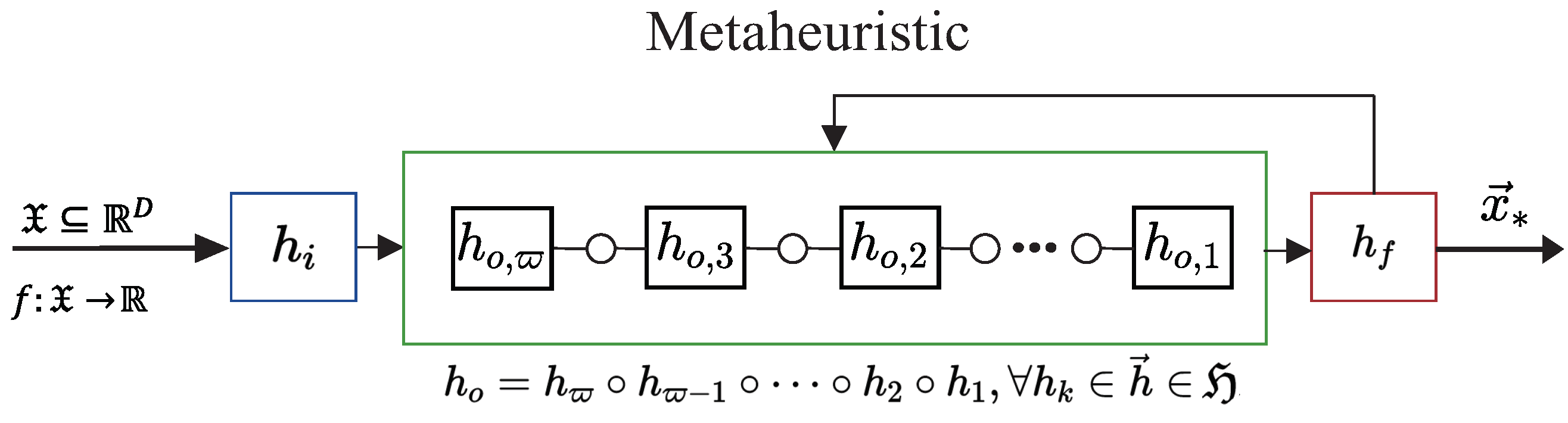
Metaheuristics (MHs) are stochastic strategies designed to control SHs. They are considered mid-level heuristics because they interact with the problem domain by controlling an iterative process that combines SHs blocks [5]. Many MHs’ mathematical foundations are associated with metaphors related to nature or physical behavior. Examples of classical MHs include Particle Swarm Optimization (PSO), Genetic Algorithm (GA), Simulated Annealing (SA), Ant Colony Optimization (ACO), and Differential Evolution (DE). However, it should be noted that some scientific community members have used metaphors to describe some of the MHs as “novel” but lacking mathematical support, while others are simply versions of established classical MHs [27,28]. In this work, the MHs are studied as functional blocks, as shown in Figure 1, based on their mathematical foundations and lack of associated metaphors. Thus, an MH has three main components: an initializer , at least one search operator , and a finalizer [9]. Following these main components, an MH can be formally defined as
where can be one or many SOs, i.e., , .

Figure 1.
Metaheuristic model represented through simple heuristics. It comprises an initializer (), one or many search operators () under the composition operation (∘), and a finalizer ().
2.2.3. Hyper-Heuristics
HHs are high-level methods that do not interact directly with the problem domain. Instead, they focus on navigating a heuristic space to find a suitable combination of SHs to obtain good solutions to a given problem [29]. The chief difference between MHs and HHs is that MHs follow a specific procedure to render a solution. Meanwhile, HHs are mechanisms that autonomously reorganize to determine the optimal arrangement of operators for addressing a specific problem [26]. Therefore, HHs are formally defined as
where Q is a metric that measures the candidate’s performance and is the candidate sequence of SHs within . There is no single formula for defining Q, as it depends on the specific objectives of the designer. For our problem, due to the stochastic nature of heuristic sequences, Q can be computed practically by combining statistics from several independent runs of in the same problem . Thus, this technique searches for the optimal heuristic configuration that best approaches the solution of with the maximal performance.
2.3. Low-Level Domain: Buck–Boost Converter Driven by Adaptive Sliding Mode Controllers
Buck–Boost converters are power electronic devices that regulate voltage levels in direct current (DC) systems. They can operate in two modes: one involves increasing the output voltage (Boost) while the other involves reducing it (Buck). This particularity makes them indispensable elements in integrating renewable energies [11] and battery energy storage [30]. In addition, Buck–Boost converters are convenient when the input voltage may fluctuate, ensuring a stable output voltage for the correct operation of the connected load.
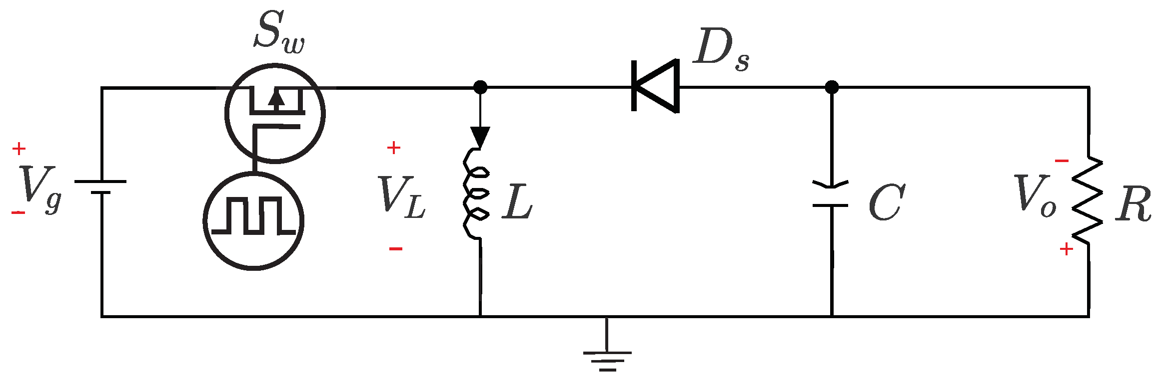
Figure 2 depicts the circuit diagram of a Buck–Boost converter. The converter is composed of an uncontrolled switching diode (), a controlled switch (), a capacitor (C [F]), an inductor (L [H]), and a resistor (R []) as load. The input voltage ( ) is supplied to the converter and can be stepped up or down depending on the switching state of . The output voltage ( ) is regulated to maintain a stable value, which can be set at levels above or below the source voltage and is often of reversed polarity.

Figure 2.
Basic circuit diagram of a DC-DC Buck–Boost converter.
The operation principle of this converter is summarized with two possible states driven by Pulse Width Modulation (PWM):
- State 1: and , when .
- State 2: and , when .
Where n is the switching cycle index, T represents the switching period, and is the PWM duty cycle. Therefore, properly adjusting the switch operating point allows us to obtain an output voltage level within the desired limits while ensuring continuous switching between states 1 and 2. The set of coupled differential equations presented in (8) describes the dynamic behavior of the Buck–Boost converter.
where [V] is the capacitor voltage, [A] represents the inductor current, and the converter output is [V]. It is essential to note that before the Laplace transform was applied, the model was scaled and nondimensionalized to simplify the analysis.
since [] and s represents the complex frequency variable. All systems and signals in the s-domain use the hat notation, e.g., . While the linearization process simplifies the analysis and enables the derivation of the transfer function shown in (9), it inherently excludes certain nonlinear and dynamic behaviors of the Buck–Boost converter. Notably, the linear model does not capture real-time switching effects and high-frequency transient dynamics intrinsic to DC-DC converters. Additionally, the model does not account for external disturbances or noise that may arise in practical implementations, such as electrical noise or input voltage fluctuations. Despite these limitations, the linearized model provides a sufficiently accurate representation to analyze the system’s dynamic response and evaluate the performance of the proposed control scheme.
Table 1 displays the component parameters considered to conduct numerical simulations for this case study.

Table 1.
Configuration of component values in the DC-DC Buck–Boost converter circuit.
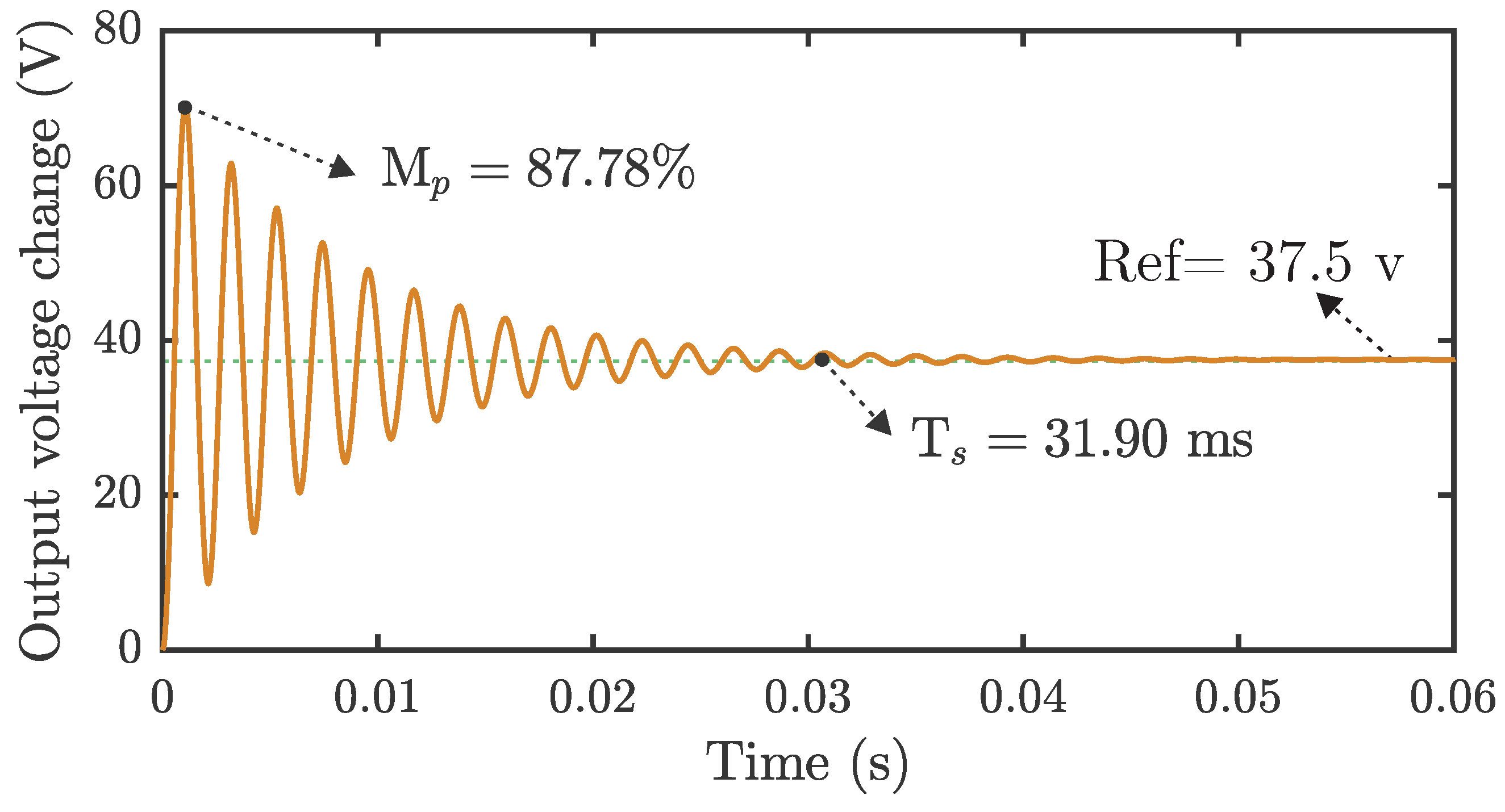
Figure 3 presents the open-loop response of the Buck–Boost converter face to a pulse input using a of . The transient response oscillates with an unacceptable overshoot (Mp = ) and a long settling time (Ts = ms). In particular, this overshoot should be corrected for most applications because it may harm electrical components and Printed Circuit Board (PCB) track insulation and reset unprotected event-driver microcontrollers.

Figure 3.
Open-loop response of the Buck–Boost converter for a pulse-shape input. The main signal features, including the overshoot (Mp), which represents how much of the reference voltage (Ref) has been exceeded, and the settling time (Ts), which indicates the amount of time required for the system to be stable, are presented.
Figure 3 also suggests that the Buck–Boost converter requires a control system to drive the response to the voltage user-defined reference. However, the control designer faces several uncertainties, such as inaccurate estimation of model parameters, nonlinearities, and external perturbations involving induced noise and currents that may destabilize the system and make this task challenging. Therefore, we decided to implement an SMC, which is robust against perturbations and disturbs, ensuring convergence in a finite time.
Nevertheless, the ASMC presents the chattering effect as the main drawback, producing uncertain behaviors in which high-frequency oscillations on the control signal may affect the proper actuators’ functioning and unbounded control gain.
It is also important to note that the mathematical model assumes ideal circuit components and neglects the effects of parasitics, such as inductor resistance or capacitor leakage, which can affect the converter’s efficiency and stability. These simplifications, while necessary to maintain the focus on the controller’s design and tuning, mean that some real-world behaviors may not be fully captured.
Hence, this study proposes using an ASMC to dynamically adapt the time-varying control gain to reject such perturbations or uncertainties.
Figure 4 shows the proposed control system applied to a Buck–Boost DC-DC converter using an ASMC.

Figure 4.
DC-DC Buck–Boost converter driven by an Adaptive Sliding Mode Controller.
The optimal controller requires the design of an accurate and reliable tuning framework. The process begins by defining the error signal (e) and its derivative over time (), as shown below,
where is the output voltage (the main state variable), and is the voltage signal reference. Notice that these two voltages are normalized to be dimensionless. Next, a sliding surface must be defined, and a manifold must be configured to dictate the system’s desired behavior. The sliding surface function () is commonly expressed according to the control objective, such as tracking e. Then, a sliding surface is defined as follows:
where is a positive design constant that defines the slope of the tracking error and affects how quickly the system can converge to the reference. It is worth mentioning that the sliding mode objective is to ensure that the sliding surface and its derivative tend smoothly to zero in a finite time, i.e., and . This action guarantees that the desired behavior will be achieved in the presence of perturbations and parametric variations. Finally, the adaptive sliding mode controller u is expressed as
where k is the adaptive gain [16], whose dynamic is given by
since and are positive parameters, the user adjusts the system’s adaptive rate and precision. Generally, the adaptive gain k is used to scale the signal in (12) adaptively. The value of k can be varied in real time to respond to changes in system conditions or to compensate for disturbances and nonlinearities. This adaptability helps maintain the desired system dynamic response and ensures that the output follows the reference accurately.
Therefore, the control tuning process involves determining the optimal values for , , and that meet the desired control response specifications. Such parameters directly influence the generation of the control signal to modify the system dynamics, thus eliciting target behavior. In the optimization context, the control design vector corresponds to . These parameters must be estimated to meet the requirements or control features shown in Table 2.
Table 2.
Desired control features for the dynamic response of the DC-DC Buck–Boost converter coupled with an Adaptive Sliding Mode Controller.
The optimization problem can be written mathematically as
since
From (15), corresponds to the optimal design vector comprising the parameters that tune the ASMC, and , , and are the regularization parameters, with values of 0.3, 1.0, and 0.7, respectively. To handle the simple constraints for the feasible region given by the limits of , the default procedure incorporated in the framework is used, which consists of detecting if a candidate solution goes outside in order to return it to the closest boundary.
Moreover, [V] is the control action signal, Mp [%] is the overshoot, Ess [V] is the steady-state error, and Ts [s] is the settling time. These features are extracted from the output voltage (cf. Figure 5), i.e., an output signal is obtained from each proposed controller. The control features from this signal are extracted and introduced into the objective function. Note that a ‘d’ is appended to each symbol’s subscript for the desired parameter. In particular, since is often set to zero, a very small value [V] is included to prevent division by zero. Lastly, the objective function utilizes a penalty function to deal with control actions greater than desired.

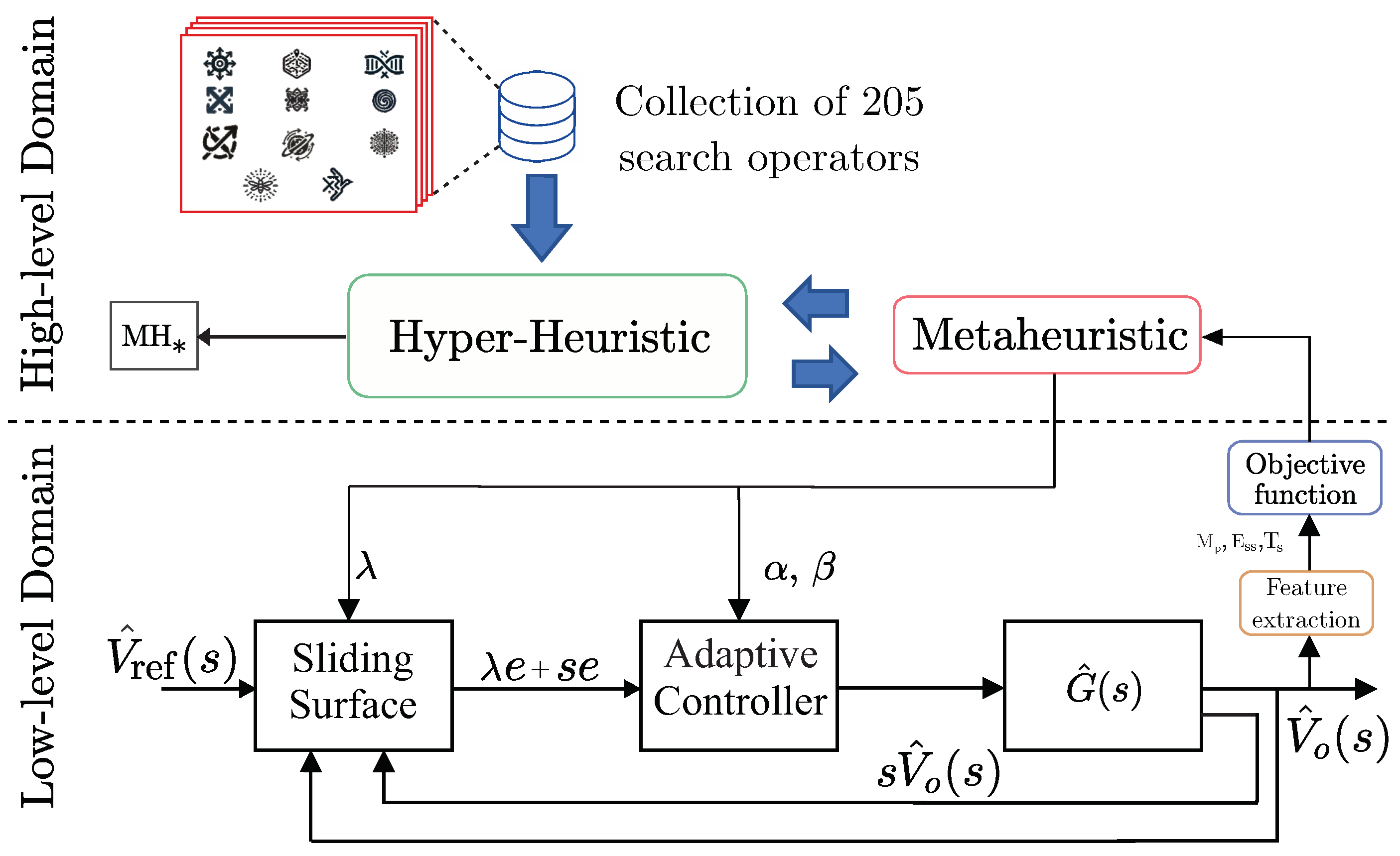
Figure 5.
Overview of the proposed framework. A hyper-heuristic approach is employed in the high-level domain to automatically obtain tailored metaheuristics using a collection of 205 search operators. In the low-level domain, an Adaptive Sliding Mode Controller is tuned, optimizing the performance of a DC-DC Buck–Boost converter.
To summarize the low-level problem domain, the objective is to force the state of the DC-DC Buck–Boost converter to track references, satisfying a settling time (Ts) with a maximum overshoot (Mp) using an optimal ASMC (). Even though the design space is limited to three variables (), the problem’s intrinsic complexity and strong nonlinearities make it challenging. Additionally, evaluating the objective function requires that time-consuming simulations be run with the candidate controller parameters and measuring the resulting system characteristics.
3. Description of the Approach
The problem addressed in this study corresponds to the Metaheuristic Composition Optimization Problem (MCOP) in (1), which is used to find the most suitable MH algorithm to tune an ASMC applied in DC-DC Buck–Boost converter systems. The low-level problem for this controller is defined in (15). Therefore, we propose automatically generating a customized MH using an HH approach that can modify the system dynamic response driven by an optimally tuned ASMC.
Algorithm 1 describes the procedure associated with the proposed methodology. The first block initializes the different parameters required for execution, including the Initial Temperature and the Cooling Rate . These parameters were selected from previous research, where the framework achieved an excellent performance for benchmark functions [10]. Next, the candidate heuristic sequence is modified and evaluated on the low-level problem in the main loop, followed by the Metropolis selection criterion. Everything is repeated until the temperature variable in SA reaches a minimum value or the procedure stalls. In this implementation, SA explores the heuristic space by randomly selecting actions from a set of actions (i.e., add, delete, and perturb) and thus finds a candidate neighbor.
| Algorithm 1 Automated Design of metaheuristics based on Simulated Annealing | |
| |
| 1: | ▹ Define the action set |
| 2: | ▹ Initialize with uniform randomly selected heuristics |
| 3: , and | ▹ Initialize other variables |
| 4: | ▹ Evaluate the performance |
| 5: while and do | |
| 6: | ▹ Randomly choose an action considering |
| 7: | ▹ Apply the action to find the candidate neighbor |
| 8: EvalPerformance | |
| 9: | ▹ Increase the stagnation counter |
| 10: if then | ▹ Metropolis selection |
| 11: and | ▹ Update the current solution |
| 12: | ▹ Reset the stagnation counter |
| 13: | ▹ Decrease the temperature |
| 14: return | ▹ Return the best metaheuristic |
| 15: function EvalPerformance() | |
| 16: | ▹ Initialize the set of solutions |
| 17: for to do | ▹ Perform repetitions required in (19) |
| 18: EvalMH | ▹ Use to solve |
| 19: | ▹ Save the current solution |
| 20: return | ▹ Return the performance using (19) |
| 21: function EvalMH() | |
| 22: | ▹ Initialize iteration counter |
| 23: | ▹ Initialize population |
| 24: | ▹ Obtain fitness values |
| 25: since | ▹ Current best |
| 26: while do | ▹ Apply the finalizer |
| 27: | ▹ Increase iteration counter |
| 28: for to do | ▹ Apply the search operators |
| 29: | ▹ Read perturbator and selector |
| 30: | ▹ Apply the oth perturbator |
| 31: | ▹ Apply the oth selector |
| 32: return | ▹ Return the best candidate solution |
The algorithmic complexity of the employed methodology is primarily influenced by the low-level simulation of the dynamic system, with an estimated cost of , where represents the number of simulation steps and denotes the time per step. So, the computational cost of the optimization process arises from the search operators, with a complexity of , where N is the population size, D is the problem’s dimensionality, and is the cost associated with the perturbation operation. Consequently, the total complexity of a complete MH run, composed of search operators and iterations, is summarized as follows:
This formulation is valid for MHs comprising a sequence of SOs, like PSO with or GA with . Now, extending this analysis to the HH methodology controlled by SA increases the complexity due to the heuristic domain search process. The algorithmic complexity of the HH framework is expressed as
where is the maximum number of steps in the SA process, is the number of repetitions required to evaluate the performance of a candidate MH, is the maximum number of iterations in the MH process, and is the maximum number of SOs employed within the HH framework. It is crucial to clarify that in (18) represents the computational cost of designing an MH, which is analogous to the training process in ML paradigms or the challenging-to-quantify effort of manually crafting algorithms using either solid theoretical foundations or nature-inspired heuristics. Once an MH has been automatically designed using the HH framework, the computational burden of applying the resulting method is reduced to in (17), as the SOs have already been identified and combined. This distinction highlights the efficiency of the automated process, where the design phase () is a one-time effort, while subsequent implementations incur only the cost of executing the custom MH ().
Figure 5 illustrates the interaction of the HH (or high-level solver) with the ASMC tuning for DC-DC Buck–Boost converter systems (or low-level problem). Although the low-level problem is three-dimensional, it is difficult to solve. Evaluating the objective function involves simulating a dynamic system with a nonlinear controller for an electrical system subject to varying operating conditions and disturbances.
Moreover, the performance of a search operator’s sequence , forming the metaheuristic () is given by
with
where med is the median and iqr represents the interquartile range statistics applied to the fitness function after implementing the MH on repetitions; thus, . Each candidate MH is evaluated 20 times (), and all fitness values are recorded to measure the performance of the MH using the metric defined in (19).
This efficient approach was previously validated using classical benchmark functions [10]. However, this study proposes adapting this framework to address real engineering problems.
4. Experimental Setup
The numerical results were coded using Python v3.9 running on Windows 10-64 bit, installed on an ASUS TUF Gaming F17 WorkStation, configured with AMD Ryzen™ 7 Processor 5700G-8 CPU Cores and 16GB RAM. The core of this project is the HH framework, known as CUSTOMHyS v1.1.6, which was used as an MH generator. This framework is freely available at https://pypi.org/project/customhys/, and it was last accessed on 31 July 2024. All data used in this work are freely available at https://github.com/Danielfz14/Mathematics_2024 (accessed on 31 July 2024).
All experiments used a collection of 205 SOs which were obtained by considering different parameters and values [10]. Table 3 contains the SOs used to build the heuristic space. It consists of 205 perturbator-derived SOs pulled from ten classic MHs in the literature, incorporating several parameter and hyperparameter variations. It also includes four selector options: Direct, Greedy, Metropolis, and Probabilistic.
Table 3.
Search operators that comprise the heuristic space with their perturbators, selectors, and hyper-parameters variants.
The low-level problem in this study mainly comprises a three-dimensional design vector , with , , and , for the ASMC. For HH implementation, each candidate MH employed a population size of 20 individuals and was limited to 30 iterations. These parameters were selected to balance exploration and exploitation while maintaining a manageable computational cost. Given the complexity of the low-level problem, tuning an ASMC for a DC-DC Buck–Boost converter using a larger population or more iterations would have significantly increased the computational burden. It is important to note that these choices were not arbitrary but were designed to align with the overall experimental framework. Furthermore, a maximum number of 10 HH steps (iterations of SA as an HH) were sufficient to generate the solver. Each SO contributing to the candidate MH represents a query to the objective function. This implies that if the MH’s cardinality is two, two evaluations of the objective function are performed in each iteration. Based on this characteristic, the number of agents and iterations were defined, ensuring an efficient use of the available computational budget. Thus, the HH aims to find a combination of operators that, within this budget, achieves a competitive performance. Several experiments were conducted to test the robustness of the achieved MH. In these experiments, two widely recognized MHs were evaluated to address the same problem, and their results were compared with those obtained by the custom MH. The selected MHs were PSO and GA. The choice of these techniques is justified, given that the custom MH integrates operators derived from both MHs. For this analysis, the GA and PSO implementations were used with the operators provided by the CUSTOMHyS framework.
The configuration specified in [9] provided the MHs operators: for PSO, was used, while for GA, were chosen. The next stage consisted of comparing the performance of our methodology with several recognized MHs, such as Multiple Adaptation Differential Evolution (MadDE) [21] and Success-History Adaptive Differential Evolution with Linear Population Size Reduction (L-SHADE) [22], which have proven to be efficient in complex optimization problems. Additionally, emerging and increasingly popular MHs were included, such as the Marine Predators Algorithm (MPA) [31] and Giant Trevally Optimizer (GTO) [32]. For these comparisons, the algorithm configuration provided by the MEALPY framework (freely available at https://pypi.org/project/mealpy/, and it was last accessed on 15 November 2024) was used to facilitate the performance evaluation in optimization problems [33]. Each method allocated a maximum of 1200 objective function evaluations to ensure a fair comparison across all implemented algorithms. Finally, we performed confirmation tests of the tuned controller using different input signals feeding the controlled DC-DC Buck–Boost converter system.
5. Experimental Results
This section presents the experimental analysis that was conducted to evaluate the proposed methodology. It is divided into three parts: Section 5.1 describes the design process of the tailored MH; Section 5.2 evaluates the performance of this MH against other methods; and Section 5.3 examines the performance of the ASMC tuned by the tailored MH in dynamic scenarios.
5.1. Hyper-Heuristic Process
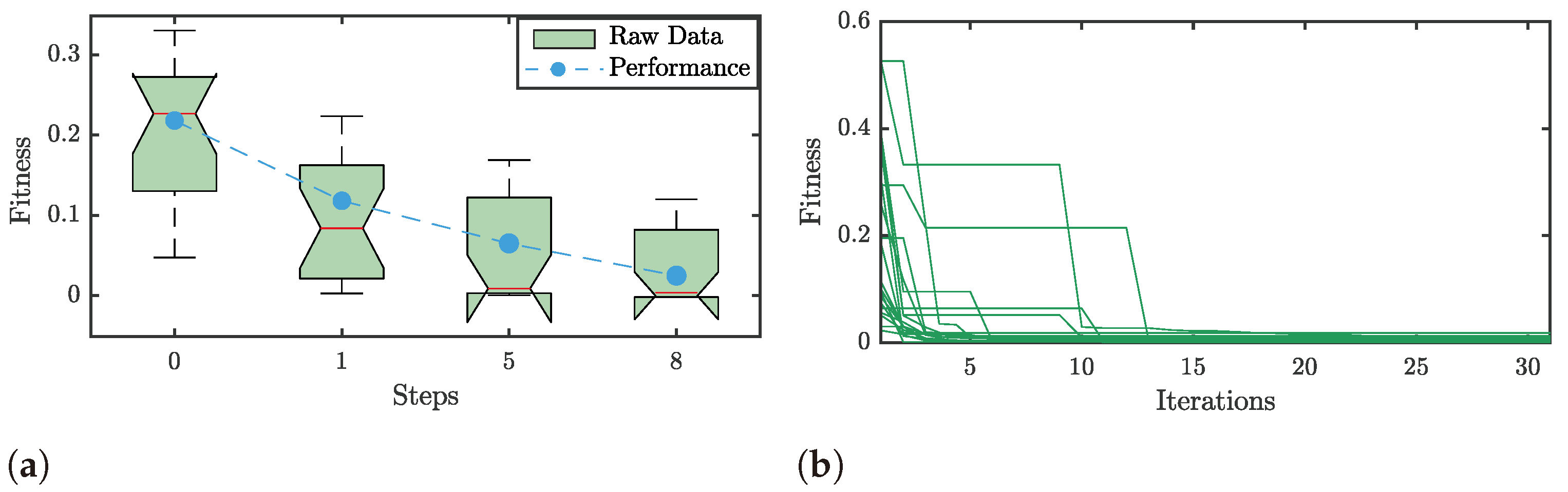
The first stage consisted of implementing the AAD-based approach and finding the solver best suited to the low-level problem, i.e., tuning an ASMC in a DC-DC Buck–Boost converter system. The HH process was then started, as shown in Figure 6a. The tendency to improve the Q performance increased as the HH steps increased (see the blue markers). Each Boxplot represents the fitness values achieved by the candidate MH after repeating the optimization process 20 times. In step 8, the HH used a combination of SOs (MH8) to perform better than the previous candidate combinations. The MH8 behavior is observed in Figure 6b, where the fitness value over multiple replicates converges rapidly and obtains values close to zero. Specifically, obtained a Q value of .

Figure 6.
(a) The tendency of the performance metric Q along the hyper-heuristic process (High-level problem), where the dashed line represents the performance evolution. (b) The behavior of the custom MH in step 8 () generated to solve the low-level problem.
Although the results are promising, the HH process was run for only ten steps, so the performance could be improved upon by allowing a more extensive scan. Detailing the composition of operators obtained by , this tailored MH presents two SOs, as shown below:
The order of these operators is crucial, i.e., . The exploration or exploitation of tailored MH depends on the order of each operator. The first search operator, , corresponds to an Inertial Swarm Dynamic perturbator using a Levy probability distribution function (pdf) to sample the random variables, which is succeeded by a direct selection. The second one, , stands for a Genetic Crossover with a blending mechanism, a tournament pairing scheme of two individuals () with a probability () of 100%, and a mating pool factor () of 0.4, followed by a Probabilistic selector with . Table 4 details the parameters of each search operator.
Table 4.
The hyper-parameters of each search operator are used to compose the tailored metaheuristic.
In this first stage, a tailored MH using an AAD-based approach was obtained, constituted by two SOs, and the first operator was based on swarm dynamics followed by a genetic crossover. Importantly, unlike a conventional hybrid algorithm combining PSO and GA, this tailored MH strategically mixes the PSO primary operator with the GA crossover operator, creating a unique combination that is tailored to the solution of the low-level problem.
To provide us with a deeper understanding of the generated MH*, a detailed procedure is presented in Algorithm 2. Recall that this procedure uses the parameter values presented in Table 4, and these additional features mentioned in Step 2 refer to those extra parameters or attributes needed for each individual in the population to implement a given search operator. For example, a velocity is used to compute a new position in PSO, a ranking list or archive is used to perform a genetic crossover, and an acceleration is used to move an individual through a gravitational force.
| Algorithm 2 Tailored Metaheuristic | |
| |
| 1: Initial iteration | |
| 2: Initialize the population positions | |
| 3: Initialize additional features for each individual in the population | |
| 4: Evaluate the population | |
| 5: Find since , | |
| 6: while False do | |
| 7: | |
| 8: for SearchOperator do | |
| 9: SearchOperator | |
| 10: Update , and the additional population features | |
| 11: return | |
| 12: procedure (X) | |
| 13: get hyper-parameters: , pdf, swarm_approach; and additional features: and | |
| 14: Evaluate | |
| 15: for do | ▹ Swarm Dynamic perturbation |
| 16: RandomSampler | |
| 17: | |
| 18: | |
| 19: | ▹ Direct Selection |
| 20: return X | |
| 21: procedure (X) | |
| 21: get hyper-parameters: , , crossover_mechanism, pairing_scheme, | |
| 22: Rank and | |
| 24: CrossoverMask | |
| 25: for do | ▹ Genetic Crossover perturbation |
| 26: Pairting | |
| 27: | |
| 28: for do | ▹ Probabilistic selection |
| 29: | ▹ |
| 30: return X | |
5.2. Tailored Metaheuristic Evaluation
Once the MH* was obtained, its performance was evaluated to determine the control features presented in Table 2. Its performance was verified by comparing it with results obtained by classical MHs from the literature, such as PSO and GA. The experiment consisted of adjusting the ASMC parameters in 20 independent replicates.
Table 5 shows the average and standard deviation of the parameters obtained for the ASMC (, , and ) and the fitness values obtained for each MH. The results indicate that MH* achieved the lowest average fitness value compared to the other methods, obtaining , followed by PSO with and GA with .
Table 5.
Average and standard deviation of design parameters and fitness values for Adaptive Sliding Mode Controllers, as optimized by MH*, PSO, and GA.
In fact, MH* achieved a fitness value that was approximately 27.57 times lower than that of PSO and 267.83 times lower than that of GA.
PSO stands out for its ability to deliver relatively good solutions, achieving a lower average fitness value () than GA and showing a minor standard deviation (), indicating better consistency in the solutions obtained. Nonetheless, our adapted MH, which includes a PSO and a GA part, outperforms the other methods in terms of robustness and fitness value.
The better performance of MH* compared to algorithms such as PSO and GA can be attributed to its composite structure, which effectively combines exploration and exploitation strategies. As shown in Table 5, MH* integrates a Swarm Dynamic Perturbation operator inspired by PSO, employing an inertial approach with a Levy distribution to enhance exploration and avoid premature convergence. Additionally, the Genetic Crossover operator facilitates exploitation by refining promising regions of the search space, while the Probabilistic Selection Mechanism dynamically balances exploration and exploitation by diversifying the search process. In contrast, PSO alone needs more refinement to be provided by the crossover operator, and GA alone suffers from limited exploration dynamics; as such, each of them is prone to suboptimal solutions in complex search spaces. By leveraging the complementary strengths of these components, MH* achieves a robust and adaptive search process, leading to improved performance across various scenarios.
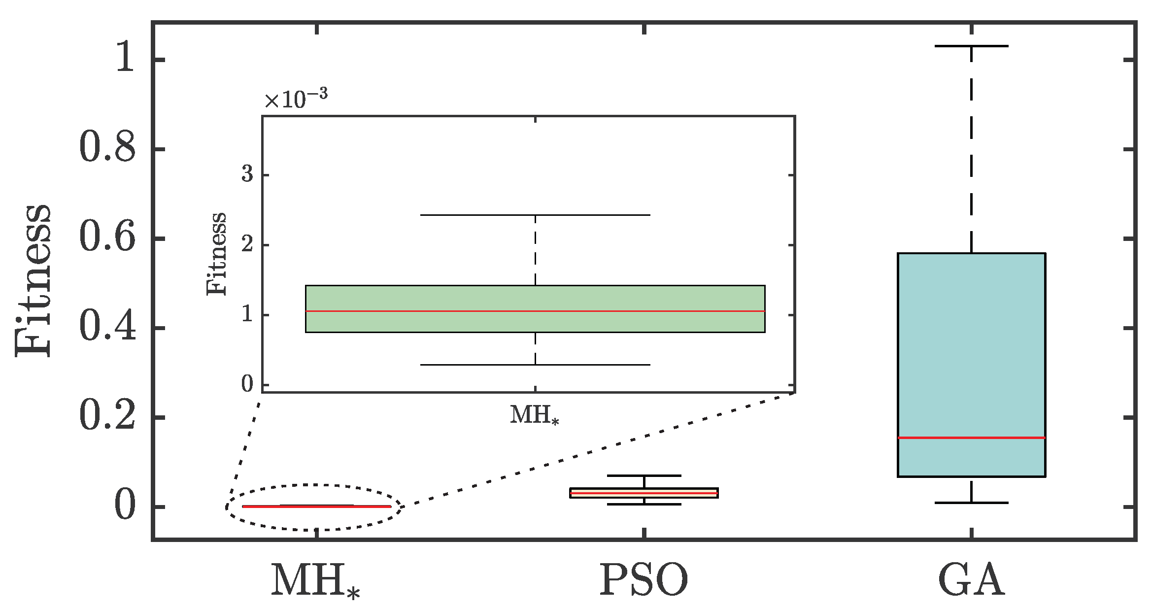
Figure 7 presents a boxplot illustrating the distribution of fitness values across the different MH methods. MH* achieved the best performance, showing minimal fitness data dispersion and high repeatability, as indicated by its narrow interquartile range (IQR) of . In contrast, the classical MHs (PSO and GA) displayed wider IQRs of and , respectively. This highlights MH*’s excellent stability and consistency compared to the other methods. PSO exhibited less dispersion than GA, making it a viable choice for scenarios requiring less stringent accuracy.

Figure 7.
Fitness values correspond to 20 controller designs achieved by the tailored (MH*) and two classical (PSO and GA) metaheuristics.
By analyzing the solutions obtained with the implemented MHs, distinct trends for the design parameters , , and were detected. Firstly, the parameter tends to take small values, especially in the case of MH*, reaching a value of . This reduction aligns well with the requirements of the optimization problem, as lower values of help minimize oscillations and smooth the control action, effectively addressing the penalty imposed on excessive control effort (15). Alternatively, the parameter showed an increasing trend, particularly in PSO, where it reached an average value of . This increase reflects a strategy aimed at aggressively reducing the steady-state error; however, it also leads to higher energy consumption by the controller, which may not be ideal in scenarios where energy efficiency is critical. Lastly, we observed relatively stable values for across all methods, with MH* slightly increasing () and the minor standard deviation among the tested algorithms. This appropriate adjustment of allows for rapid error correction while avoiding excessive control effort, balancing rapid response and system robustness.
Avoiding constant saturation states and excessive power consumption is essential in practical applications. In this context, precise adjustment of the controller parameters is required, allowing the adaptive gain to be dynamically adjusted according to the converter’s needs. The sensitivity of the controller parameters in maintaining proper converter response is worth noting. Although a detailed sensitivity analysis is beyond the scope of this work, MHs represent a vital tool in this context, as they facilitate the exploration of configurations that would be unattainable through traditional methods such as trial and error. Any modification in controller parameters or gains can directly impact the operating characteristics of the converter, affecting critical metrics such as overshoot (Mp), settling time (Ts), and steady-state error (Ess).
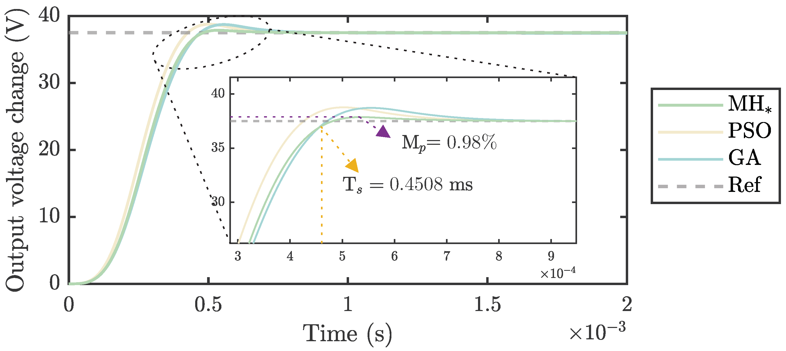
Figure 8 provides a clear example of this behavior. The tailored MH* achieved the best performance with an overshoot () and a fast settling time ( ms), as highlighted in the inset. The MH*, PSO, and GA controller parameters were set to the average values of 20 independent runs. In contrast, PSO and GA exhibited higher overshoot and longer settling times, aligning with the fitness values increase observed in Table 5.

Figure 8.
Step response of the DC-DC Buck–Boost converter in a closed-loop configuration with an Adaptive Sliding Mode Controller (ASMC) tuned using MH*, PSO, and GA. The ASMC parameters were set to the average values in Table 5, obtained from 20 independent runs.
Figure 8 shows how the MH*-tuned controller meets the requirements requested in Table 2. The overshoot reduction from to stands out among the improvements. Also, the controlled system achieves a stabilization time of 0.4508 ms. Finally, the steady-state error for the Heaviside-type input was reduced to zero.
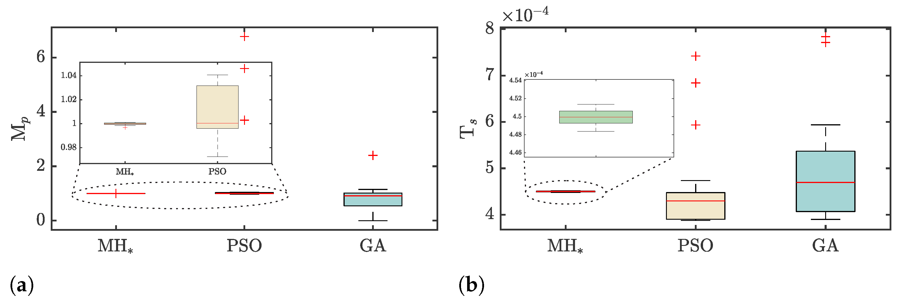
The controller’s performance can be better understood by conducting a detailed analysis of the overshoot behavior across all replicates, as illustrated in Figure 9a. It is pertinent to mention that the tailored MH demonstrates high repeatability, obtaining an average overshoot of 0.9997%. In contrast, PSO shows an overshoot of 1.655%, while GA exhibits a considerably higher overshoot, reaching 0.8102%. M* achieved an overshoot with a median of 0.9998% and a low dispersion (IQR %), demonstrating its high robustness and accuracy. On the other hand, PSO’s performance was also remarkable, reaching a median value close to 1%, although it presented a higher variability, which was reflected in an IQR of 0.035%. This behavior is expected, given that PSO contains one of the critical components of the custom metaheuristic MH*. Finally, GA presented the poorest performance, with a median of 0.91% and considerable dispersion (IQR %).

Figure 9.
(a) Overshoot ( [%]) and (b) Settling Time (Ts [s]) values for the Adaptive Sliding Mode Controller tuned by the tailored (MH*) and two classical (PSO and GA) metaheuristics, corresponding to 20 controller designs.
A similar trend for the settling time is observed, as shown in Figure 9b. The tailored MH* met the design objective, achieving a median settling time of ms with minimal variability (IQR = ms). Although PSO achieved a slightly shorter median settling time ( ms), it deviated from the target specified in the objective function. It exhibited significantly higher variability with an IQR of ms. In contrast, GA presented the longest settling time, with a median of ms and the highest dispersion (IQR = ms).
In addition to the initial tests, further experiments were conducted using robust algorithms renowned for their excellent performance in various optimization competitions, such as MadDE, L-SHADE, and emerging swarm-type MHs, including MPA and GTO. These algorithms were selected based on their strong exploration capabilities, as demonstrated by the consistent performance of similar approaches like PSO. Plus, it is worth mentioning that all four algorithms (L-SHADE, MadDE, MPA, and GTO) are population-based MHs built upon foundational methods like Differential Evolution (DE). Each algorithm adapts its core mechanisms to enhance performance and balance exploration and exploitation. L-SHADE and MadDE employ archives and historical information within complex, hybridized structures of search operators grounded in theoretical principles. In contrast, MPA and GTO derive their mechanisms from diverse phenomena, such as predation and optics, relying heavily on nature-inspired metaphors to frame their approaches.
Table 6 summarizes the outcomes of the experiment mentioned above, where MH*, MadDE, and L-SHADE demonstrate highly competitive performances. The strong results of MadDE and L-SHADE are expected, as experts in the optimization field meticulously crafted these algorithms and have consistently proven their efficiency in tackling various problems. On the other hand, it is remarkable that MH* achieved comparable performance without manual intervention, as it was automatically generated through an AAD-based approach. It is worth noticing that L-SHADE and MadDE utilize more than two search operators and rely on data-driven mechanisms to adjust their hyperparameters [21,22] dynamically. While these features enhance their optimization potential, they also incur significantly higher computational costs than MH*.
Table 6.
Fitness metrics for each MH, including best fitness, median fitness, Standard Deviation (STD), interquartile range (IQR), and p-value from statistical comparisons with MH*.
In particular, MH* achieved the best fitness value of , with a median of and an IQR of , indicating low variability and robust performance. L-SHADE rendered a competitive fitness value of and a median of but with higher variability reflected in an IQR of . Similarly, MadDE achieved a minimal fitness of and a median of , though with greater scatter, as evidenced by a standard deviation of . In contrast, MPA and GTO demonstrated inferior performance across multiple replicates, although they obtained good results in specific scenarios. Both algorithms exhibited more significant variability in their outcomes, with IQRs of for MPA and for GTO. Moreover, a nonparametric statistical test, specifically the one-sided Wilcoxon signed-rank test, was conducted to verify the reliability of the results presented in Table 6 for MH* and the other metaheuristics. The null (H0) and alternative (H1) hypotheses were defined as follows:
H0.
Heuristic-based tuner A performs as well as or worse than heuristic-based tuner B.
H1.
Heuristic-based tuner A outperforms heuristic-based tuner B.
The p-values obtained from the Wilcoxon signed-rank test for comparisons between MH* and the other metaheuristics (MadDE, L-SHADE, MPA, and GTO) were all below the significance threshold of : for MadDE, for L-SHADE, for MPA, and for GTO. These results allow us to reject H0 and accept H1, confirming that MH* outperforms the tested algorithms.
Beyond statistical significance, evaluating the practical implications of these findings is paramount. MH* demonstrates competitive performance and exceptional consistency, as evidenced by its lower IQR and standard deviation compared to the other methods. This consistency is particularly critical in industrial applications, where variability can jeopardize process stability and product quality. Therefore, considering the inherent complexity of these optimization problems, particularly with regard to identifying regions of convergence that meet specific control requirements, MH*’s robust performance and reliability accentuate its potential for addressing real-world engineering challenges.
5.3. Performance of ASMC Tuned by a Tailored Metaheuristic
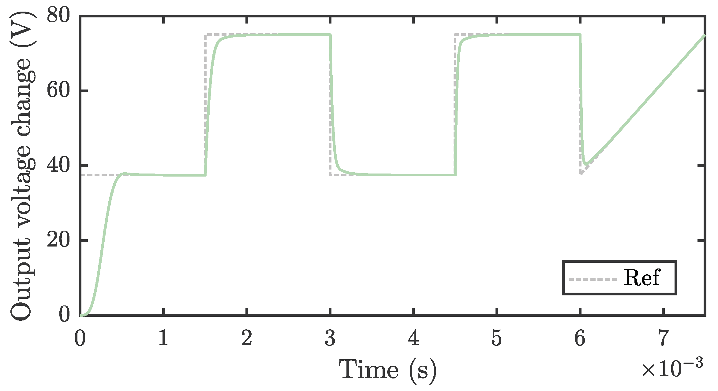
The last stage involved evaluating the tuned controller’s performance; the mean values obtained for , , and found in the previous tests were selected for this test. Figure 10 sketches the transient response of the output voltage in a DC-DC Buck–Boost converter when the input voltage exhibits step and ramp behaviors. The green trace represents the converter’s output voltage signal, while the gray curve signifies the target reference voltage. The converter’s output voltage responds effectively to abrupt changes in input voltage, emulating these transients without overshoot and long settling times. During ramped inputs, the output voltage rises steadily, with minimal latency, reflecting the precise tuning of the ASMC. The balance between accuracy and a speedy response is essential in applications that require voltage regulation in the face of load fluctuations or input variables.

Figure 10.
The output voltage of the Buck–Boost DC-DC converter, controlled by an ASMC tuned with MH*, is shown for different input voltage profiles, including step and ramp functions.
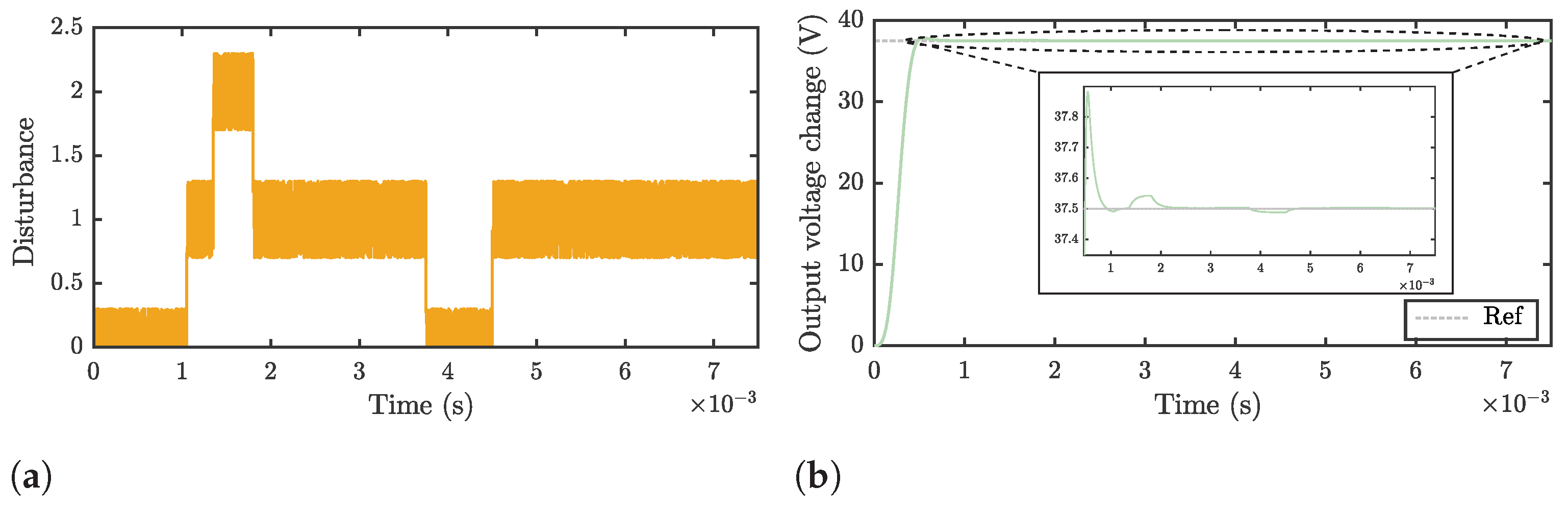
The disturbance test is another crucial examination that can be used to verify the robustness and proper functionality of the optimally adjusted ASMC. To this end, a disturbance scenario was simulated wherein the DC-DC Buck–Boost converter was subjected to a nonlinear load profile. This scenario diverges from the ideal conditions and is symbolic of real-world industrial operations where the system’s misalignment of several active components is prevalent. For instance, in an industrial setting, the converter may suddenly face a nonlinear load profile caused by the activation of a high-power industrial motor within a production line. Such motors, equipped with variable-speed drives, generate significant electrical noise and impose fluctuating power demands on the system. These fluctuations often manifest as rapid changes in current consumption, leading to pronounced voltage dips and surges, which can compromise system stability and the performance of sensitive equipment. Figure 11a illustrates the aforementioned nonlinear load profile deployed as the perturbation signal. The profile is characterized by abrupt and significant load alterations, embodied by various peaks, posing a considerable challenge to any control system. Due to its nonlinear characteristics, this disturbance tends to reverberate throughout the system, potentially precipitating severe complications without a competent controller.

Figure 11.
(a) Disturbance signal representing a nonlinear load profile connected to the controlled system. (b) Response to nonlinear perturbations achieved by the DC-DC Buck–Boost converter controlled by the Adaptive Sliding Mode Controller tuned with the tailored metaheuristic (MH*).
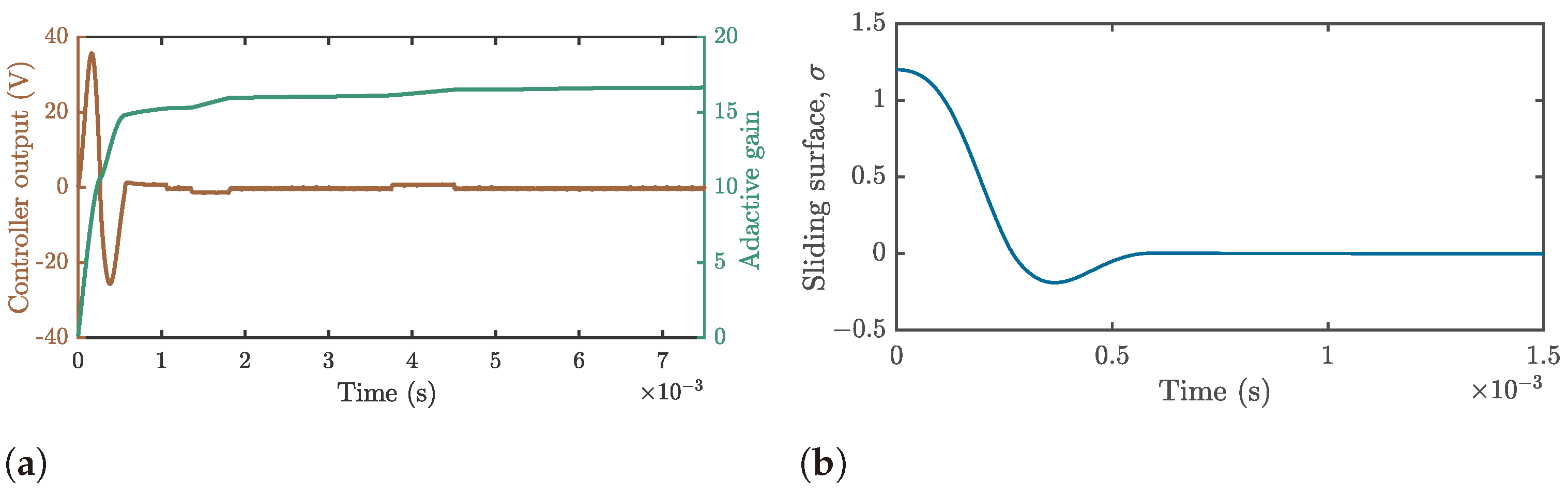
Nonetheless, the adaptive control mechanism ensures that the Buck–Boost converter’s response remains within acceptable parameters for various applications, as depicted in Figure 11b. It indicates that in conjunction with the ASMC, the converter can sustain an output voltage within close vicinity of the target voltage, notwithstanding load perturbations. While minor fluctuations in the output voltage are observable upon disturbance, they are promptly rectified. The zoomed-in view in Figure 11b offers further insight into the converter’s performance under disturbances, confirming that the voltage is consistently regulated to ensure that it remains close to the reference value. Lastly, to achieve the system response shown in Figure 11b, it was necessary to generate a control action signal to mitigate the disturbances entering the system. If unobserved, this control action can reach very high values at the simulation level, which is forbidden in practical scenarios. Figure 12a shows the controller’s response and adaptive gain in an ASMC in the presence of nonlinear disturbances. The control action signal (brown traces) initially shows a rapid increase, seeking to minimize the error and achieve the reference value, then stabilizes with only minor fluctuations.

Figure 12.
Analysis of the Adaptive Sliding Mode Controller performance under nonlinear perturbations: (a) Control action signal and adaptive gain variation and (b) behavior of the sliding surface function.
On the other hand, the adaptive gain delivers small increases (green traces) generated by the disturbance, and later becomes stable. The control action is maintained within the operating limits, and the gain is adjusted, ensuring system equilibrium without exceeding the energy parameters defined in the optimization problem formulation. This result indicates that this control signal can be implemented in a real scenario. Plus, it is essential to highlight that such a response was rendered from the generated slip surface presented in Figure 12b. The behavior of this sliding surface function was as expected because it converges to zero in finite time without being affected by the nonlinear perturbations introduced to the system. This behavior substantiates the efficacy of our controller’s calibration.
6. Conclusions
In this study, we developed and analyzed an Automated Algorithm Design (AAD) methodology with a practical emphasis on solving real-world optimization challenges. The focus was on tuning an Adaptive Sliding Mode Controller (ASMC) for a DC-DC Buck–Boost converter, which is a vital element in numerous electrical systems. To tackle this optimization problem, we automatically generated a tailored population-based metaheuristic (MH*) using Simulated Annealing Hyper-Heuristic (SAHH) as a high-level strategy.
The resulting MH* configuration integrates an inertial particle swarm operator from PSO, a Levy distribution used to sample random values, and a genetic crossover operator from GA, followed by a probabilistic selection mechanism. This composite structure allows MH* to leverage the strengths of both exploration and exploitation phases, providing a balanced search capability that is tailored to the tuning requirements of ASMC. Our results revealed that the ASMC tuned by the tailored MH*, generated using an AAD approach, achieved a highly satisfactory performance. The average controller parameter values obtained from 20 independent runs were , , and . This configuration significantly improved the system’s dynamic response, reducing overshoot from 887.78% to an average of 0.98%, i.e., an approximately 90-fold improvement. Similarly, the settling time was reduced from 31.90 ms to an average of 0.4508 ms, corresponding to a 71-fold reduction. Comparative tests were also conducted to evaluate the tailored MH* against classical MHs such as PSO and GA and advanced methods like MadDE, L-SHADE, and emerging MHs such as MPA and GTO. The results indicate that the AAD-designed MH* delivered competitive outcomes, achieving comparable or superior performance in various scenarios. This claim is evident from the Standard Deviation (STD) and interquartile Range (IQR) values shown in Table 6. For example, MH* achieved an IQR of and an STD of , reflecting consistent solutions with low dispersion, outperforming MPA (IQR = , STD = ) and GTO (IQR = , STD = ). Plus, statistical tests corroborated the competitiveness of MH*. The p-values obtained in the Wilcoxon signed-rank test for comparisons with other algorithms were all below , confirming the statistically significant superiority of MH* across the tested scenarios.
Moreover, this ASMC exhibited rapid and effective disturbance rejection, ensuring agility and efficacy in responding to unexpected variations. Its adaptability and resilience to nonlinear external perturbations highlight its stability and robustness, even under varying operational conditions. Its ability to quickly mitigate disturbances while maintaining stability emphasizes the reliability of this approach when applied to complex processes. The results confirm the effectiveness and versatility of the proposed methodology, demonstrating its potential to deliver tailored solutions for real-world engineering problems. This approach empowers professionals with limited optimization expertise to design efficient MHs that address specific challenges effectively. Furthermore, using these tuned controllers, or an embedded version of MH*, could indirectly reduce hardware operating costs and decrease heat dissipation, enhancing overall system efficiency and longevity. We foresee multiple avenues for future research building on the proposed methodology. One promising direction is to broaden the scope of this approach by applying it to a broader range of real-world engineering problems, thereby evaluating the performance of automatically generated MHs in scenarios closely aligned with their original design objectives.
Additionally, recent advancements in Machine Learning (ML) methods, particularly reinforcement learning and neural network-based optimization, have shown promise in control system applications. These methods could complement the AAD framework by providing dynamic, real-time adaptability with regard to the selection and tuning of heuristic operators. Incorporating ML into future iterations of AAD could enable more intelligent, data-driven decision-making processes, enhancing its performance in highly nonlinear and time-varying control systems. Another compelling path involves developing a more sophisticated high-level solver with enhanced capabilities for exploring the heuristic space. These features could include the ability to detect patterns and correlations between operators, optimizing their selection for specific applications. Progressing along these lines holds the potential to make significant contributions to the AAD field, fostering innovation and practical advancements in engineering optimization.
Author Contributions
Data curation, J.M.C.-D. and H.C.; Formal analysis, J.G.A.-C.; Investigation, D.F.Z.-G., J.M.C.-D., H.C. and J.G.A.-C.; Methodology, D.F.Z.-G.; Software, D.F.Z.-G.; Validation, J.M.C.-D., H.C. and J.G.A.-C.; Writing—original draft, D.F.Z.-G.; Writing—review and editing, J.M.C.-D., H.C. and J.G.A.-C. All authors have read and agreed to the published version of the manuscript.
Funding
This work was supported by the Research Group in Advanced Artificial Intelligence at Tecnológico de Monterrey, grant NUA A00836756; the Mexican Council of Humanities, Sciences, and Technologies (CONAHCyT) under scholarship 1046000 and the University of Guanajuato CIIC (Convocatoria Institucional de Investigación Científica, UG) project 243/2024.
Institutional Review Board Statement
Not required for this study.
Informed Consent Statement
No Formal written consent was required for this study.
Data Availability Statement
Data available under a formal demand.
Conflicts of Interest
The authors declare no conflicts of interest.
Abbreviations
| Acronyms | |
| AAD | Automated Algorithm Design |
| ASMC | Adaptive Sliding Mode Controller |
| DC-DC | Direct Current to Direct Current |
| DE | Differential Evolution |
| GA | Genetic Algorithm |
| GTO | Giant Trevally Optimizer |
| HH | Hyper-Heuristic |
| IQR | Interquartile range of the fitness values |
| L-SHADE | Success-History Adaptive Differential Evolution with Linear Population Size Reduction |
| MadDE | Multiple Adaptation Differential Evolution |
| MCOP | Metaheuristic Composition Optimization Problem |
| MH | Metaheuristic |
| ML | Machine Learning |
| MPA | Marine Predators Algorithm |
| PCB | Printed Circuit Board |
| PSO | Particle Swarm Optimization |
| PWM | Pulse Width Modulation |
| SA | Simulated Annealing |
| SAHH | Simulated Annealing Hyper-Heuristic |
| SH | Simple Heuristic |
| SMC | Sliding Mode Controller |
| SO | Search Operator |
| STD | Standard deviation of the fitness values |
| Mathematical Operators and Functions | |
| Time derivative operator | |
| iqr | Interquartile range operator |
| Laplace transform operator | |
| med | Median operator |
| Probability distribution function | |
| ∘ | Composition operator |
| Metaheuristic and Optimization Symbols | |
| Low-level minimization problem representation | |
| A | Action set of simple heuristics for combinatorial problem domains |
| Add | Heuristic that inserts a new element into the current sequence |
| D | Dimensionality or number of decision variables |
| Cooling rate | |
| F | Set of fitness values obtained after evaluating each solution in |
| Objective function to minimize | |
| Heuristic sequence of search operators | |
| Constructive heuristic | |
| Feasible heuristic space | |
| Finalization heuristic or finalizer | |
| Initialization heuristic or initializer | |
| Search operator composed of a perturbator and selector, | |
| Optimal candidate heuristic sequence within | |
| Perturbation heuristic or perturbator | |
| Selection heuristic or selector | |
| Heuristic space with operators | |
| MHk | Metaheuristic based on the heuristic sequence |
| N | Population size |
| Stagnation threshold | |
| Number of repetitions for performance evaluation | |
| Maximum cardinality of the action set | |
| Per | Heuristic that perturbs an element in the current sequence |
| Q | Performance function to maximize |
| D-dimensional real-valued domain | |
| S | Arbitrary element within |
| Feasible arbitrary domain | |
| Arbitrary domain of an optimization problem | |
| Initial temperature | |
| Temperature variable | |
| Minimum temperature | |
| Maximum number of iterations | |
| Cardinality or number of search operators | |
| Position within | |
| Feasible domain of the low-level optimization problem | |
| Set of solutions obtained after independent repetitions of implementing a given MH | |
| Optimal solution within | |
| Control System and Application-Specific Symbols | |
| Control action signal | |
| Desired control action signal | |
| Dimensionless parameter to adjust the adaptive dynamic | |
| Dimensionless parameter to adjust the adaptive dynamic | |
| Capacitor | |
| Duty cycle | |
| Diode | |
| e | Dimensionless error signal or difference between output and reference voltages |
| Very small value to prevent division by zero | |
| Desired steady-state error | |
| Steady-state error | |
| Switching frequency | |
| Dimensionless transfer function of the system | |
| G | Dimensionless impulse function of the system |
| Inductor current | |
| k | Adaptive gain |
| Inductor | |
| Dimensionless constant of the sliding surface | |
| Desired peak overshoot | |
| Peak overshoot | |
| P | Penalty function related to the control action signal |
| Resistor | |
| s | Dimensionless complex frequency variable |
| Sliding surface function | |
| Switch | |
| T | Switching period |
| Desired settling time | |
| Settling time | |
| u | Adaptive sliding mode controller |
| Optimal adaptive sliding mode controller | |
| Capacitor voltage | |
| Input or source voltage | |
| Output voltage | |
| Dimensionless reference voltage | |
| Reference voltage | |
| Regularization parameter in the tuning problem, | |
References
- Joseph, S.B.; Dada, E.G.; Abidemi, A.; Oyewola, D.O.; Khammas, B.M. Metaheuristic algorithms for PID controller parameters tuning: Review, approaches and open problems. Heliyon 2022, 8, e09399. [Google Scholar] [CrossRef] [PubMed]
- Altbawi, S.M.A.; Mokhtar, A.S.B.; Jumani, T.A.; Khan, I.; Hamadneh, N.N.; Khan, A. Optimal design of Fractional order PID controller based Automatic voltage regulator system using gradient-based optimization algorithm. J. King Saud Univ.-Eng. Sci. 2021, 34, 1–13. [Google Scholar] [CrossRef]
- Zhao, S.; Zhang, T.; Ma, S.; Chen, M. Dandelion Optimizer: A nature-inspired metaheuristic algorithm for engineering applications. Eng. Appl. Artif. Intell. 2022, 114, 105075. [Google Scholar] [CrossRef]
- Fathi, M.; Khezri, R.; Yazdani, A.; Mahmoudi, A. Comparative study of metaheuristic algorithms for optimal sizing of standalone microgrids in a remote area community. Neural Comput. Appl. 2022, 34, 5181–5199. [Google Scholar] [CrossRef]
- Hussain, K.; Mohd Salleh, M.N.; Cheng, S.; Shi, Y. Metaheuristic research: A comprehensive survey. Artif. Intell. Rev. 2019, 52, 2191–2233. [Google Scholar] [CrossRef]
- Pereira, I.; Madureira, A.; Costa e Silva, E.; Abraham, A. A hybrid metaheuristics parameter tuning approach for scheduling through racing and case-based reasoning. Appl. Sci. 2021, 11, 3325. [Google Scholar] [CrossRef]
- Isiet, M.; Gadala, M. Sensitivity analysis of control parameters in particle swarm optimization. J. Comput. Sci. 2020, 41, 101086. [Google Scholar] [CrossRef]
- Vlad, A.I.; Romanyukha, A.A.; Sannikova, T.E. Parameter Tuning of Agent-Based Models: Metaheuristic Algorithms. Mathematics 2024, 12, 2208. [Google Scholar] [CrossRef]
- Cruz-Duarte, J.M.; Ortiz-Bayliss, J.C.; Amaya, I.; Shi, Y.; Terashima-Marín, H.; Pillay, N. Towards a Generalised Metaheuristic Model for Continuous Optimisation Problems. Mathematics 2020, 8, 2046. [Google Scholar] [CrossRef]
- Cruz-Duarte, J.M.; Amaya, I.; Ortiz-Bayliss, J.C.; Conant-Pablos, S.E.; Terashima-Marín, H.; Shi, Y. Hyper-Heuristics to customise metaheuristics for continuous optimisation. Swarm Evol. Comput. 2021, 66, 100935. [Google Scholar] [CrossRef]
- Hasanpour, S.; Baghramian, A.; Mojallali, H. Analysis and Modeling of a New Coupled-Inductor Buck–Boost DC–DC Converter for Renewable Energy Applications. IEEE Trans. Power Electron. 2020, 35, 8088–8101. [Google Scholar] [CrossRef]
- Sariyildiz, E.; Yu, H.; Ohnishi, K. A practical tuning method for the robust PID controller with velocity feed-back. Machines 2015, 3, 208–222. [Google Scholar] [CrossRef]
- Chen, Y.S.; Hung, Y.H.; Lee, M.Y.J.; Chang, J.R.; Lin, C.K.; Wang, T.W. Advanced Study: Improving the Quality of Cooling Water Towers’ Conductivity Using a Fuzzy PID Control Model. Mathematics 2024, 12, 3296. [Google Scholar] [CrossRef]
- Huang, Y.J.; Kuo, T.C.; Chang, S.H. Adaptive sliding-mode control for nonlinearsystems with uncertain parameters. IEEE Trans. Syst. Man Cybern. Part B (Cybern.) 2008, 38, 534–539. [Google Scholar] [CrossRef] [PubMed]
- Rabiee, H.; Ataei, M.; Ekramian, M. Continuous nonsingular terminal sliding mode control based on adaptive sliding mode disturbance observer for uncertain nonlinear systems. Automatica 2019, 109, 108515. [Google Scholar] [CrossRef]
- Alvaro-Mendoza, E.; Gonzalez-Garcia, A.; Castañeda, H.; De León-Morales, J. Novel adaptive law for super-twisting controller: USV tracking control under disturbances. ISA Trans. 2023, 139, 561–573. [Google Scholar] [CrossRef]
- Hussain, K.; Salleh, M.N.M.; Cheng, S.; Naseem, R. Common benchmark functions for metaheuristic evaluation: A review. JOIV Int. J. Inform. Vis. 2017, 1, 218–223. [Google Scholar] [CrossRef]
- Hassan, A.; Pillay, N. Hybrid metaheuristics: An automated approach. Expert Syst. Appl. 2019, 130, 132–144. [Google Scholar] [CrossRef]
- López-Ibáñez, M.; Dubois-Lacoste, J.; Cáceres, L.P.; Birattari, M.; Stützle, T. The irace package: Iterated racing for automatic algorithm configuration. Oper. Res. Perspect. 2016, 3, 43–58. [Google Scholar] [CrossRef]
- Hutter, F.; Hoos, H.H.; Leyton-Brown, K.; Stützle, T. ParamILS: An automatic algorithm configuration framework. J. Artif. Intell. Res. 2009, 36, 267–306. [Google Scholar] [CrossRef]
- Biswas, S.; Saha, D.; De, S.; Cobb, A.D.; Das, S.; Jalaian, B.A. Improving differential evolution through Bayesian hyperparameter optimization. In Proceedings of the 2021 IEEE Congress on Evolutionary Computation (CEC), Krakow, Poland, 28 June–1 July 2021; pp. 832–840. [Google Scholar]
- Tanabe, R.; Fukunaga, A.S. Improving the search performance of SHADE using linear population size reduction. In Proceedings of the 2014 IEEE Congress on Evolutionary Computation (CEC), Beijing, China, 6–11 July 2014; pp. 1658–1665. [Google Scholar]
- Alfaro-Fernández, P.; Ruiz, R.; Pagnozzi, F.; Stützle, T. Automatic algorithm design for hybrid flowshop scheduling problems. Eur. J. Oper. Res. 2020, 282, 835–845. [Google Scholar] [CrossRef]
- Zhao, Q.; Duan, Q.; Yan, B.; Cheng, S.; Shi, Y. Automated design of metaheuristic algorithms: A survey. arXiv 2023, arXiv:2303.06532. [Google Scholar]
- Cruz-Duarte, J.M.; Ortiz-Bayliss, J.C.; Amaya, I.; Pillay, N. Global Optimisation through Hyper-Heuristics: Unfolding Population-Based Metaheuristics. Appl. Sci. 2021, 11, 5620. [Google Scholar] [CrossRef]
- Pillay, N.; Qu, R. Hyper-Heuristics: Theory and Applications; Springer: Cham, Switzerland, 2018. [Google Scholar]
- de Armas, J.; Lalla-Ruiz, E.; Tilahun, S.L.; Voß, S. Similarity in metaheuristics: A gentle step towards a comparison methodology. Nat. Comput. 2022, 21, 265–287. [Google Scholar] [CrossRef]
- Tzanetos, A.; Dounias, G. Nature inspired optimization algorithms or simply variations of metaheuristics? Artif. Intell. Rev. 2021, 54, 1841–1862. [Google Scholar] [CrossRef]
- Burke, E.K.; Hyde, M.R.; Kendall, G.; Ochoa, G.; Özcan, E.; Woodward, J.R. A Classification of Hyper-Heuristic Approaches: Revisited. In Handbook of Metaheuristics; Gendreau, M., Potvin, J.Y., Eds.; International Series in Operations Research & Management Science; Springer International Publishing: Cham, Switzerland, 2019; pp. 453–477. [Google Scholar] [CrossRef]
- Lee, H.S.; Yun, J.J. High-efficiency bidirectional buck–boost converter for photovoltaic and energy storage systems in a smart grid. IEEE Trans. Power Electron. 2018, 34, 4316–4328. [Google Scholar] [CrossRef]
- Faramarzi, A.; Heidarinejad, M.; Mirjalili, S.; Gandomi, A.H. Marine Predators Algorithm: A nature-inspired metaheuristic. Expert Syst. Appl. 2020, 152, 113377. [Google Scholar] [CrossRef]
- Sadeeq, H.T.; Abdulazeez, A.M. Giant trevally optimizer (GTO): A novel metaheuristic algorithm for global optimization and challenging engineering problems. IEEE Access 2022, 10, 121615–121640. [Google Scholar] [CrossRef]
- Van Thieu, N.; Mirjalili, S. MEALPY: An open-source library for latest meta-heuristic algorithms in Python. J. Syst. Archit. 2023, 139, 102871. [Google Scholar] [CrossRef]

Disclaimer/Publisher’s Note: The statements, opinions and data contained in all publications are solely those of the individual author(s) and contributor(s) and not of MDPI and/or the editor(s). MDPI and/or the editor(s) disclaim responsibility for any injury to people or property resulting from any ideas, methods, instructions or products referred to in the content. |
© 2024 by the authors. Licensee MDPI, Basel, Switzerland. This article is an open access article distributed under the terms and conditions of the Creative Commons Attribution (CC BY) license (https://creativecommons.org/licenses/by/4.0/).