Abstract
Continuous glucose monitoring data have strong time variability as well as complex non-stationarity and nonlinearity. The existing blood glucose concentration prediction models often overlook the impacts of residual components after multi-scale decomposition on prediction accuracy. To enhance the prediction accuracy, a new short-term glucose prediction model that integrates the double decomposition technique, nonlinear marine predator algorithm (NMPA) and deep extreme learning machine (DELM) is proposed. First of all, the initial blood glucose data are decomposed by variational mode decomposition (VMD) to reduce its complexity and non-stationarity. To make full use of the decomposed residual component, the time-varying filter empirical mode decomposition (TVF-EMD) is utilized to decompose the component, and further realize complete decomposition. Then, the NMPA algorithm is utilized to optimize the weight parameters of the DELM network to avoid any fluctuations in prediction performance, and all the decomposed subsequences are predicted separately. Finally, the output results of each model are superimposed to acquire the predicted value of blood sugar concentration. Using actual collected blood glucose concentration data for predictive analysis, the results of three patients show the following: (i) The double decomposition strategy effectively reduces the complexity and volatility of the original sequence and the residual component. Making full use of the important information implied by the residual component has the best decomposition effect; (ii) The NMPA algorithm optimizes DELM network parameters, which can effectively enhance the predictive capabilities of the network and acquire more precise predictive results; (iii) The model proposed in this paper can achieve a high prediction accuracy of 45 min in advance, and the root mean square error values are 5.2095, 4.241 and 6.3246, respectively. Compared with the other eleven models, it has the best prediction accuracy.
Keywords:
blood glucose concentration; double decomposition; nonlinear marine predator algorithm; deep extreme learning machine; prediction MSC:
68Q07; 68T07
1. Introduction
With the continuous improvement in people’s quality of life, the incidence of diabetes has shown an increasing trend. Chronic diabetes can lead to a variety of complications and can be life-threatening in severe cases [1]. Therefore, the accurate prediction and effective management of fluctuations in blood sugar levels are essential for diabetes treatment [2]. An excellent blood glucose prediction algorithm not only reduces the incidence of hyperglycemia and hypoglycemia, but also combines with insulin pumps to regulate insulin dosage [3]. By finding the optimal pumping time, the algorithm can achieve the precise control of blood sugar in diabetic patients.
The continuous blood glucose monitoring system (CGMS) is a novel blood sugar monitoring method widely used in clinical practice [4], as shown in Figure 1. CGMS is a technology that uses glucose sensors to detect glucose levels in subcutaneous interstitial fluid. This technology can reflect the changes and fluctuations in human blood sugar in a more comprehensive and detailed way [5]. Researchers discovered that utilizing data obtained by CGMS to predict blood sugar levels over time could significantly reduce the probability of having high or low blood sugar [6]. Therefore, the forecasting of blood sugar levels is currently a hot topic within the domain of diabetes therapy.
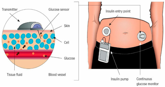
Figure 1.
CGMS collection process diagram.
At present, the research methods of blood sugar forecasting can be separated into two categories: one approach relies on physiological mechanisms [7], and the other utilizes a data-driven approach [8,9,10]. On account of the complexity of the physiological mechanism, there are numerous factors affecting blood sugar levels, which makes it difficult to build a precise blood sugar prediction model. Meanwhile, the study also discovers that the physiological blood sugar forecasting model is not only complicated, but also brings some time delay [11]. Common blood glucose prediction methods are data-driven and do not need to consider the regulatory mechanism of the human body. Only the historical blood sugar concentration data measured by patients can be utilized to build a model to predict future blood sugar changes [12,13]. At present, the prediction technology based on the CGMS measurement data mainly includes the autoregressive model [14], extreme learning machine (ELM) [15], support vector machine [16], recurrent neural network (RNN) [17] and long short-term memory network (LSTM) [18]. Deep learning has a strong nonlinear fitting ability and is widely applied in the forecasting of blood sugar concentration [19,20,21,22]. When dealing with large amounts of complex data, it can achieve better results than traditional machine learning technologies. It can be utilized to capture the nonlinear properties of blood glucose concentration series and make predictions using these properties to more accurately predict outcomes. LSTM is a popular deep neural network within the domain of time series forecasting. By introducing the memory unit and gating mechanism, LSTM can address the issues of gradient vanishing and gradient exploding in the long sequence data of the RNN network [23]. Notwithstanding the fact that LSTM performs well in blood glucose prediction, it possesses numerous hyperparameters that require adjustment, which greatly increases the complexity and training difficulty of the network. Especially when dealing with large amounts of data, the training time and computing costs rise significantly. DELM combines the advantages of deep learning and ELM to simplify the network structure to a large extent [24]. The method of random initialization is adopted during training, which greatly reduces the number of hyperparameters to be tuned and improves the efficiency of training [25]. Moreover, the training process of DELM is relatively simple and does not require repeated iteration and optimization, so the training time is short. Nonetheless, the predictive performance of DELM is susceptible to alterations in weight parameters [26,27]. At present, a large number of heuristic optimization algorithms are used to acquire the optimal combination of weight parameters. NMPA is a novel heuristic optimization algorithm introduced by Ali in 2022 [28] on the basis of the MPA algorithm. It draws inspiration from the theory of the marine survival of the fittest, and has the advantages of high efficiency, robustness, and strong global search ability. In this paper, the NMPA method is applied to optimize the weight parameters of the DELM network. At the same time, the signal decomposition technology is introduced into the model, which can efficiently diminish the nonlinearity and non-stationarity of blood sugar concentration series [29]. Common signal decomposition techniques include wavelet transform (WT) [30], empirical mode decomposition (EMD) [31] and variational mode decomposition (VMD) [32,33]. The WT method needs to select the appropriate function and the appropriate quantity of decomposition layers in advance, which shows a serious lack of adaptability. The EMD method is adaptive and free of subjective interference, but it is prone to end effect and mode aliasing. The VMD method has stronger anti-noise ability, effectively solves the end effect and mode aliasing phenomenon and can decompose the modal components more accurately [34]. However, the VMD method produces a residual component after the decomposition of the blood glucose concentration sequence. The residual component carries rich information of the original blood glucose concentration sequence. Existing methods often discard the residual component, resulting in the incomplete decomposition of the original blood glucose data, which affects the prediction ability of the whole model. In this paper, the TVF-EMD method is used to decompose the residual component, thereby extracting the information in the original blood glucose series more completely.
In this article, a new combined model for predicting blood glucose concentration is proposed, which combines the double decomposition strategy, NMPA algorithm and DELM network. Firstly, VMD method is employed to decompose the collected blood sugar concentration sequence, and a set of relatively stable subsequences are obtained. At the same time, the TVF-EMD algorithm is employed to decompose the residual component after VMD decomposition again, fully extracting the information encompassed within the component, and realizing the complete decomposition of the original blood glucose concentration sequence. Secondly, the NMPA-DELM model is constructed to predict all the subsequences after decomposition. Finally, all subsequence predicted values are added to derive the ultimate prediction result of blood glucose data. The contribution and innovation of this paper are manifested as follows:
- (a)
- In the forecasting of short-term blood glucose concentration data, the double decomposition method is adopted to decompose the original blood glucose sequence and the generated residual component, effectively reducing the non-stationarity and non-linearity of the sequence. The overall prediction accuracy of the model with full consideration of residual component is higher.
- (b)
- The DELM network is utilized for predicting blood glucose data, which significantly improves the ability to acquire the characteristics of blood glucose concentration in depth. Furthermore, the training procedure of DELM is relatively uncomplicated, and the random initialization method accelerates the training speed, so as to achieve the high-precision prediction effect in a short time.
- (c)
- The NMPA algorithm adopts new parameters to adjust the predator’s moving step size in the process of optimization, which can maintain a high exploration ability. In the second stage, a control parameter is introduced to balance the development and exploration aspects of the algorithm, and further enhance the global and local search capabilities. Compared with the MPA algorithm, the probability of realizing that the global optimal value is greatly improved.
- (d)
- The NMPA algorithm is employed to optimize the weight parameters of DELM network and establish the optimal parameter combination model, which is helpful to avoid large fluctuations in the forecasting outcomes, improve the predictive performance of the model and make it more stable and effective.
The remainder of this article is arranged as follows. Section 2 presents the theoretical background of the VMD method, TVF-EMD method, NMPA algorithm and DELM network. In Section 3, the double decomposition and NMPA-DELM method are introduced, and the detailed steps for implementing the proposed model are also included. In Section 4, the experimental data are introduced, and the model’s predictive effect is discussed in depth compared with the prediction results of other models. At the same time, according to the evaluation index, the corresponding prediction error is analyzed, and the key factors to enhance the forecasting precision of the model are found out. Section 5 contains the summaries of the conclusions and the follow-up research tasks.
2. Decomposition and Prediction Algorithm Theory
2.1. VMD Algorithm
The VMD is a technique for decomposing signals that decomposes a known complex input signal into preset modal components with distinct center frequencies and limited bandwidth. The method determines the central frequency and bandwidth of each component by iteratively searching for the optimal solution of the variational problem. In this way, the frequency domain of the signal can be divided adaptively and each component can be separated effectively.
The aim of VMD is to minimize the total estimated bandwidths of the decomposed components, and transform it into a constrained variational problem. The corresponding center frequency is extracted, employing the alternate multiplier method. The variational problem needs to satisfy the following constraints:
where and denote, respectively, the modal component and the corresponding center frequency. is the convolution operation. is the input signal. represents the Dirac function.
To address the above optimization issue, the Lagrange operator and quadratic penalty factor are utilized to convert the constrained problem into an unconstrained problem, and the augmented Lagrange expression is obtained:
Then, the alternating direction method of multipliers (ADMM) is employed to tackle the above problem, and each component and its center frequency are constantly updated. Finally, the saddle point of the unconstrained problem is obtained, which is the optimal solution of the original problem. Each component can be estimated from the solution in the frequency domain, and the solution formula is as follows:
where , and represent the Fourier transform of , and .
can be regarded as the Wiener filtering of modal components. Within the algorithm, the center frequency is reassessed according to the center of gravity of the power spectrum of each component, and is updated by Equation (4):
2.2. TVF-EMD Algorithm
The TVF-EMD method, introduced by Li et al. in 2017 [35], is a very effective signal decomposition method that adaptively determines the quantity of decomposition layers through a convergence criterion. A time-varying filter is introduced on the basis of traditional EMD to improve the performance of its decomposition. The TVF-EMD method not only effectively avoids the problems of mode mixing and excessive modes, but also significantly improves the frequency separation performance and stability at low sampling rates. The solving steps of the TVF-EMD algorithm are outlined below:
- (1)
- Compute the local cutoff frequency.
Firstly, the instantaneous amplitude and the instantaneous frequency of the input signal are calculated according to the Hilbert transform, and then the maximum and minimum values of the local instantaneous amplitude are determined. The extreme value points of the instantaneous amplitude are interpolated, and the sequences and are obtained, respectively. Calculate the instantaneous mean and the instantaneous envelope :
At the same time, using the local extremum of the instantaneous frequency through the interpolation process, and are obtained and the instantaneous frequency components and are calculated:
Finally, the local cutoff frequency is calculated.
- (2)
- Signal reconstruction.
Rearrange to address the effect of the intermittent component and reconstruct it according to the adjusted cutoff frequency to obtain a new signal :
Based on the extreme point of as the node of the time-varying filter, the input signal is approximated by B-spline interpolation, and the outcome is obtained.
- (3)
- Solve the cut-off criterion
Given the bandwidth threshold , if condition is satisfied, the signal is locally narrowband and can be considered a component signal. If it is not satisfied, then make and repeat the above steps.
where represents the instantaneous frequency of each component of the weighted average; represents the Loughlin instantaneous bandwidth of the component signal.
2.3. Deep Extreme Learning Machine
The ELM is a single-layer neural network that randomly generates the weight and threshold of the hidden layer during the training process. The output weight can be calculated only through the generalized inverse matrix theory, and the unique optimal solution can be obtained. Therefore, it has a fast training speed and better generalization performance. However, when the data contain large noise or excessively high dimensions, it is difficult to realize the in-depth mining of the inherent information.
As a typical unsupervised learning algorithm, the autoencoder can copy the input information to the output data through training, so that the input and output of the network are the same. The idea of the autoencoder is integrated into ELM to construct the extreme learning machine-autoencoder (ELM-AE). ELM-AE is specially designed for processing high-dimensional complex data and feature learning, thereby achieving more efficient feature information extraction. When the number of nodes of the input and the hidden layer of ELM-AE are equal, equal-dimensional representation is achieved, and the output weight is solved as follows:
where denotes the hidden layer output matrix; denotes the output matrix of the output layer.
When the quantity of nodes in the input layer is greater than the quantity of nodes in the hidden layer, the compressed representation is realized, and vice versa for a sparse representation. For compressed and sparse representations, the output weight solution is expressed as:
where denotes the unit matrix; denotes the regularization coefficient; and denotes the input matrix.
DELM is a deep learning network stacked by multiple ELM-AEs [36]. Compared with traditional ELMs, DELM can more comprehensively portray the mapping relationship between data, which not only enhances the model nonlinear fitting ability, but also improves the prediction effect. The reconstruction error is minimized through hierarchical unsupervised training, so that the inputs and outputs are as close as possible during model training. Moreover, unlike common deep learning algorithms, DELM has no reverse fine-tuning process, which greatly reduces the training time. The structure of the DELM is depicted in Figure 2.
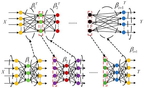
Figure 2.
DELM structure diagram.
During the training of DELM, the original input data serve as the desired output for the first ELM-AE, thereby obtaining the output weight matrix. Then, it is used as the input matrix of the second ELM-AE, and the output of the previous layer is used as the input of the next layer. This process is carried out layer by layer until the output weight matrix of the last layer is obtained, completing the entire training process.
2.4. Marine Predator Algorithm
MPA is a novel meta-heuristic optimization algorithm [37]. The algorithm draws inspiration from the theory of marine survival of the fittest and simulates the evolutionary rendition of predators and prey in the ocean. The predator achieves the optimization goal by choosing the best foraging strategy between Lévy flight or Brownian motion.
The optimization process is initiated by randomly initializing the positions of prey within the search area. The initialization process can be described as follows using a random number generator to generate initial solutions that are dispersed as evenly as feasible within the designated search area:
where and represent the lower and upper bounds of the designated search area, and represents randomly generated number in the range of .
According to the different speed ratios of prey and predators, the MPA optimization process divides the whole life cycle into three stages, namely the high-speed ratio, the equal-velocity ratio and the low-velocity ratio stage. Let and represent the current and maximum iterations, respectively.
The high-speed ratio phase occurs in the early stages of the iteration process, where the prey surpasses the predator in speed. The prey obeys Brownian motion for exploration, while the predator’s best strategy is to stay put. During this phase, the mathematical model of the population is:
where represents the moving step length; is a Brownian motion random vector with a normal distribution; is the term-by-term multiplication operator; represents an elite matrix of top predators; is the prey matrix; is a constant of 0.5; and is a uniform random number vector between 0 and 1.
The equal-speed ratio phase occurs in the middle stages of the iteration , when the prey and predator have the same speed. Meanwhile, the population is evenly divided into two parts. The former, as prey, is responsible for exploitation based on the Lévy flight strategy. The latter, as predator, is responsible for exploration based on Brownian motion and the gradual transition from exploration to exploitation. The mathematical model for the first half of the population is:
where denotes a vector that is randomly generated according to the Lévy distribution.
The mathematical model for the latter half of the population is:
where serves as an adjustable factor that controls the predator’s movement stride length.
The bottom-speed ratio phase occurs later in the iteration, when the predator surpasses the prey in speed. The predator utilizes a development strategy that mimics Lévy flight. Its mathematical model is as follows:
Research into the real-life factors that affect the foraging patterns of marine predators has found that vortex formation and fish aggregation device (FAD) effects can alter prey behavior. After updating the prey position in each iteration, MPA uses the position updating strategy based on vortex formation and FADs to further process the prey position in order to effectively avoid the result falling into the local optimal solution. Setting longer jumps in the optimization search process overcomes the premature convergence problem and thus escapes local extremes. The mathematical model is:
where is a binary vector containing only 0 and 1; is the random number between ; is a constant with a value of 0.2, indicating the probability of being affected by the FADs effect; and are randomly selected individuals.
3. Construction of the Model Using Double Decomposition and Deep Extreme Learning Machine Optimized by Nonlinear Marine Predator Algorithm
3.1. Double Decomposition Strategy
In order to dig out the variation rule of blood glucose concentration more deeply, the double decomposition strategy is applied to the prediction of blood glucose concentration, and effective signal processing technology is utilized to enhance the accuracy of the blood glucose concentration prediction results. Firstly, the VMD method is employed to decompose the original blood sugar concentration sequence to simplify the non-stationarity and complexity of individual sequences and acquire the primary characteristics of the blood glucose concentration for the follow-up of effective forecasting. The selection of the number of decomposition layers K in the process of VMD decomposition is directly related to the decomposition effect of VMD. The optimal number of decomposition layers is determined as 6 by the method of minimum envelope entropy. Building on the VMD decomposition of the original blood glucose concentration data, the residual component’s rich information is fully utilized by applying TVF-EMD for further decomposition. This approach enables a more comprehensive decomposition of the blood glucose data and enhances the model’s predictive performance.
The quantity of decomposition layers of the VMD method is 6, and the results are shown in Figure 3a. IMF1~IMF6 is the component generated after the decomposition of the entire primitive blood sugar concentration sequence, and residual is the residual component generated during treatment. It can be found that this component still contains part of the important information of the original blood sugar sequence data. On the basis of the decomposition of the original blood sugar concentration sequence data by VMD, the rich information of the residual part is fully considered and TVF-EMD is applied to decompose it again. The outcomes are presented in Figure 3b. IMF1~IMF9 are the components generated after processing the residual part. This allows the original blood glucose series to be completely decomposed, thereby improving in the anticipated effect of this model.
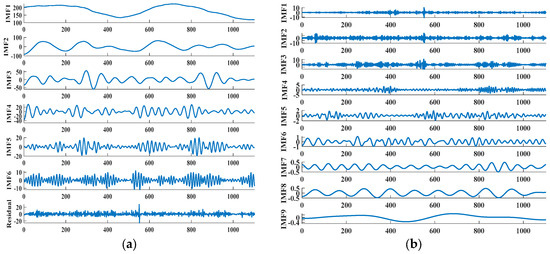
Figure 3.
Decomposition results of original blood glucose sequence and residual component: (a) VMD; and (b) TVF-EMD.
As a tool for measuring signal complexity, permutation entropy can be applied to validate the efficacy of the double decomposition strategy. The main characteristics of permutation entropy include simple calculation, strong anti-noise and anti-interference ability. Compared with traditional complexity measurement methods, such as the Lyapunov index, permutation entropy has better real-time and robustness. The specific principle of its solution is as follows:
For the phase space reconstruction of one-dimensional time series , we can obtain:
where is the embedding dimension and is the delay time.
The matrix consists of rows, each representing a reconstruction component, totaling components. Each reconstructed component is then reorganized in ascending order, determining the column index of each element’s position within the vector, thereby generating a series of symbol sequences.
where and . There are types of symbol sequences mapped in the -dimensional phase space.
The probability of occurrence for each symbol sequence can be determined by dividing the count of its occurrences by the total count of occurrences for the distinct symbol sequence, that is, . Then, the permutation entropy can be expressed in the following manner:
The value of maximum permutation entropy is , which is normalized to obtain:
where is the normalized permutation entropy. As the entropy decreases, the sequence becomes simpler and more regular. Conversely, as entropy increases, the time series exhibits greater complexity and randomness.
The principle is applied to calculate the component entropy after the decomposition of the VMD method, and the specific outcomes are presented in Figure 4a. It can be seen from the figure that the permutation entropy of the original blood glucose sequence is much higher than that of other IMF components. The entropy of the original sequence is about twice as high as the minimum entropy of all components. The results show that the complexity and non-stationarity of the original glucose concentration sequence can be effectively reduced by the decomposition of the VMD method. The residual component generated after the VMD method is decomposed by TVF-EMD, and the result is presented in Figure 4b. As depicted in the figure, the permutation entropy of the residual component is relatively large. This indicates that the residual component is highly complex and has obvious non-stationarity. After the residual component is decomposed by TVF-EMD, the permutation entropy values of the nine components obtained show an obvious decreasing trend. Moreover, the permutation entropy values of most components decrease significantly. This indicates that the TVF-EMD method significantly reduces the complexity and non-stationarity of this residual component.
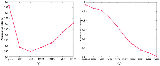
Figure 4.
The permutation entropy of components after different decomposition treatments: (a) VMD; and (b) TVF-EMD.
3.2. NMPA-DELM Method
3.2.1. Nonlinear Marine Predator Algorithm
MPA is an optimization algorithm that simulates the behavior of predators and prey in marine ecosystems. When solving complex optimization problems, it has some shortcomings, such as low precision, sluggish convergence rate and susceptible to falling into local extreme values in the later stage. Based on this, the NMPA method incorporates a novel adaptive parameter to control the predator’s moving step length. The adjustment of this parameter is intended to further improve the balance between exploration and development. By improving the global search ability in the whole optimization process, the NMPA algorithm can achieve the goal of finding the global optimal. The expression of the new adaptive parameter is presented as such:
At the same time, the NMPA algorithm also adopts the strategy of adaptively changing the inertia weight dependent on the quantity of iterations. For the early iteration, the larger inertia weight improves the global search ability. The algorithm requires local fine search in the subsequent iteration process, so the low inertia weight can strengthen the local search ability and accelerate the convergence speed. The expression of the nonlinear adaptive inertia weight is as follows:
In the process of algorithm optimization, the position update method of the high-speed ratio stage population remains unchanged. The position update of the population in the equal-speed ratio stage not only incorporates nonlinear adaptive inertia weight , but also adopts a new adaptive parameter . The mathematical model of the first half of the population will update the original Formulas (17) and (18) to:
The mathematical model of the latter half of the population is also updated with a new adaptive parameter , and the original Formulas (19) and (20) is updated to:
In addition, new adaptive parameter is also updated in the bottom-speed ratio stage, and the original Formulas (22) and (23) is updated to:
Finally, for the influence of environmental factors such as eddy current or FADs effect, new adaptive parameters are also updated. After each iteration, the original position update strategy is still maintained to further process the prey position. The original Formula (24) is updated to:
3.2.2. Construction of NMPA-DELM
In ELM-AE, the weights of the input layer are randomly initialized and remain unchanged during the training process, which is very easy to cause the performance of DELM network to fluctuate and the prediction accuracy to decline. By using the NMPA algorithm to optimize the weight parameters of DELM, the prediction accuracy and stability can be effectively improved. The process of NMPA-DELM model is displayed in Figure 5. The specific steps are outlined as follows:
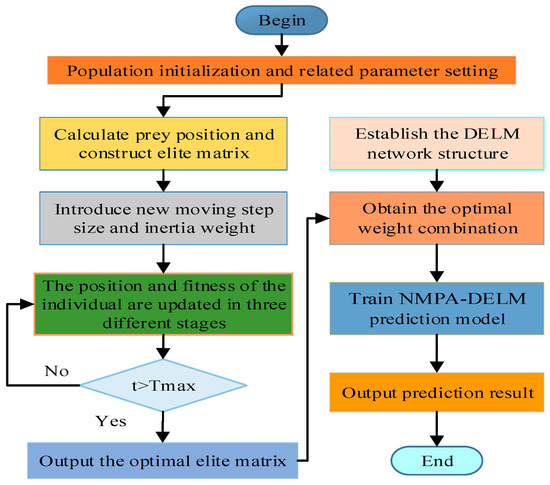
Figure 5.
Flowchart of NMPA-DELM model.
- (1)
- Set the parameters of NMPA, encompassing the population number , maximum number of iterations , variable dimension and search scope .
- (2)
- Population initialization: The ownership values are combined as the position of each prey, and the position of the individual prey population is initialized by Formula (14).
- (3)
- The mean square error between the real value and the predicted value is used as the fitness function to calculate and rank the fitness value of the prey individual. Through this process, the individual with the best fitness is found out and the elite matrix is constructed.
- (4)
- The prey position is updated in the high-speed ratio stage, equal-speed ratio stage and low-speed ratio stage, memory storage and elite update are realized and new adaptive moving step parameters and inertia weights are calculated. For vortex or FAD effects, the prey is updated using Equation (34).
- (5)
- Determine whether the maximum number of iterations has been reached. If yes, the iteration ends and the best elite matrix is entered into the DELM as a combination of weights. Otherwise, skip to step 3.
3.3. Prediction of Blood Glucose Concentration Based on Double Decomposition and NMPA-DELM
The flowchart of the blood sugar concentration forecasting model using the double decomposition and nonlinear marine predation algorithm for optimizing the DELM model is depicted in Figure 6, with the following steps:
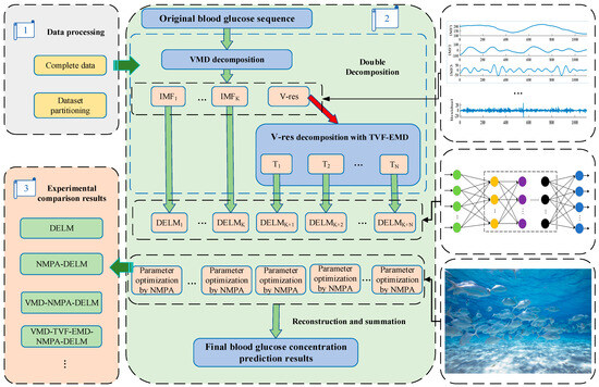
Figure 6.
Structure diagram of VMD-TVF-EMD-NMPA-DELM model.
- (1)
- Decompose the original blood sugar concentration data using the VMD method to acquire a series of smoother modal components.
- (2)
- The residual component after VMD processing is calculated and the component is decomposed using the TVF-EMD method. In this way, the complexity of the fluctuation of the residual component is reduced and the double decomposition results are obtained.
- (3)
- The NMPA algorithm is employed to optimize the weight parameters of the DELM network and find the most effective parameter combination, so as to avoid the volatility of the network prediction performance.
- (4)
- Input all the components into the NMPA-DELM network for training separately to obtain the predicted values of each subsequence.
- (5)
- Merge the forecasting outcomes of all sub-sequences to obtain the ultimate predicted sequence of blood sugar concentration.
4. Experimental Simulation Analysis
4.1. Sources and Configurations for Blood Glucose Concentration Data
The data used in this paper come from a publicly accessible study (https://public.jaeb.org/direcnet/stdy/ (accessed on 5 December 2023)). This is the continuous blood glucose measurement value collected by CGMS on the Diabetes Research in Children Network (DirecNet), in which the patients are children with type 1 diabetes. In this article, blood glucose concentration data from three patients (NO. 12, NO. 71 and NO. 84) were randomly selected from this study. The data are sampled at 5 min intervals, and the length of the series is over 1000. Figure 7 shows the raw blood glucose data for patients NO. 12, NO. 71 and NO. 84, respectively, and it is clear that the blood glucose concentration values are a strongly time-varying time series, with a great deal of nonlinearity and non-stationarity. The blood glucose data are divided, with the proportion of the training set being 70% and the proportion of the test set being 30%. The length of the window for input data is 10, which is the blood glucose values collected by the patient for the past 50 min. The forecast horizon is set to 45 min. The prediction error is reduced by averaging the results of multiple experiments. All the prediction experiments involved are implemented in MatlabR2021A.
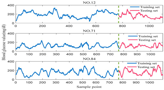
Figure 7.
Raw blood glucose concentration data from different patients.
4.2. Model Performance Evaluation Index
To assess the predictive capability of VMD-TVF-EMD-NMPA-DELM model more comprehensively, this paper adopts Clarke Error Grid Analysis (CEGA) [38] and three commonly used error evaluation indexes. These are mean absolute percentage error (MAPE), mean absolute error (MAE) and root mean square error (RMSE) [39,40]. When the error index value is low, it means that the deviation between the forecasted value and observed value is small, and the prediction performance of the corresponding model is better. All indicators are calculated as follows:
where denotes the quantity of test samples; and and are the forecasted and observed values at the corresponding time, respectively.
CEGA evaluates the precision of the forecasting method by analyzing the probability of the blood glucose estimate falling in five regions A, B, C, D and E. The more points falling in region A, the better the prediction performance of this method. For the error evaluation index, when its value is low, it means that the discrepancy between the predicted and observed values is small, and the prediction performance of this corresponding model is better.
4.3. Ablation Study
In order to verify the effectiveness of the VMD-TVF-EMD-NMPA-DELM prediction model proposed in this paper, ablation studies were conducted on each module of the model. The VMD-TVF-EMD-NMPA-DELM prediction model was used to predict blood glucose concentration in diabetic patients. The four models were used to predict blood glucose 45 min in advance. The error performance of the four prediction models 45 min in advance for different patients was analyzed. The MAE, RMSE and MAPE performance indicators of different prediction methods are shown in Table 1.

Table 1.
Prediction error indicators of each model 45 min in advance.
From the results in Table 1, it can be observed that, for different patients, the values of the three indicators in the NMPA-DELM model are all lower than those in the DELM prediction model. The MAE, RMSE and MAPE of the NMPA-DELM model are reduced by 4.6685, 3.3774 and 3.9792% at most, respectively. This indicates that optimizing the key parameters of the DELM model using the NMPA algorithm can obtain more accurate prediction results. Compared with the prediction results of the NMPA-DELM model, the VMD-NMPA-DELM model has better MAE, RMSE and MAPE values. After introducing VMD decomposition, the MAE, RMSE and MAPE of the model are reduced by 17.0365, 23.9079 and 10.4135% at most, respectively. This indicates that decomposing before prediction can effectively reduce the non-stationarity and nonlinearity of the original blood glucose. Compared to direct prediction results, its prediction accuracy is higher. Comparing the results of the VMD-TVF-EMD-NMPA-DELM model and VMD-NMPA-DELM model, the former has higher prediction accuracy. The MAE, RMSE and MAPE of the VMD-TVF-EMD-NMPA-DELM model are reduced by 1.3251, 1.4641 and 0.8647% at most, respectively. This indicates that fully utilizing the important information of residual components and effectively reducing their complexity and volatility can further improve the predictive performance of the model. By comparing the data in Table 1, it can be seen that the VMD-TVF-EMD-NMPA-DELM model in this paper has the smallest MAE, RMSE and MAPE, indicating that the proposed model has the best predictive performance. The proposed VMD-TVF-EMD-NMPA-DELM model has the best predictive performance, with all three performance indicators lower than the other three prediction models.
The error indicators bar chart and CEGA diagram of the blood glucose prediction results of each model for different patients are shown in Figure 8. At the same time, the blood glucose prediction results and error curves of each model for different patients 45 min in advance are plotted, as shown in Figure 9.
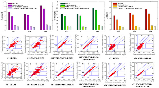
Figure 8.
The error indicators bar chart and CEGA diagram of each model.
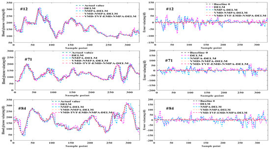
Figure 9.
Prediction results and error curves of each model.
As can be seen from Figure 8 and Figure 9, the predicted values and actual values of the VMD-TVF-EMD-NMPA-DELM model proposed in this paper are very close for different patients. At the same time, the prediction error and performance indicators of this model are significantly smaller than the other three models. In addition, the proportion of the predicted values of the VMD-TVF-EMD-NMPA-DELM model falling in area A in the CEGA diagram is also the highest. The results show that the VMD-TVF-EMD-NMPA-DELM model has the best prediction performance.
4.4. Comparison Between NMPA Algorithm and Other Optimization Algorithms
Using the NMPA algorithm to optimize the weight parameters of the DELM model can significantly improve the prediction accuracy and overall performance of the model. In order to further verify the advantages of the NMPA algorithm, the optimization results of this algorithm are compared with the genetic algorithm (GA), particle swarm optimization algorithm (PSO), sparrow search algorithm (SSA) and MPA algorithm, respectively. The GA-DELM, PSO-DELM, SSA-DELM, MPA-DELM and NMPA-DELM models are used to predict the blood glucose concentration 45 min in advance for different patients. The results of the three performance indicators of all models are shown in Table 2.
Table 2.
Performance index results of prediction errors of each model.
From Table 2, it can be seen that, compared with the results of the other four models, the NMPA-DELM model has the smallest MAE, RMSE and MAPE values. This indicates that the predictive performance of the NMPA-DELM model is superior to the other four models. Among these algorithms, the NMPA algorithm has a higher optimization ability and obtains the optimal parameter combination for the DELM network. Among these five models, the GA-DELM model has the worst prediction accuracy. Compared with the prediction results of the GA-DELM model, the MAE, RMSE and MAPE of NMPA-DELM model are reduced by 3.1791, 1.733 and 2.5263% at most, respectively. Compared with other optimization algorithms, the optimized model of NMPA algorithm shows lower error values, indicating its significant advantage in improving the prediction accuracy.
The MAE, RMSE and MAPE indicator bar chart and CEGA diagrams of the prediction results of the five models are plotted, as shown in Figure 10. The blood glucose prediction results and error curves graphs of different models for different patients 45 min in advance are also included, and the changes are shown in Figure 11.
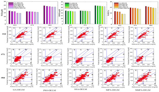
Figure 10.
The MAE, RMSE and MAPE bar chart and CEGA diagrams of the prediction results.
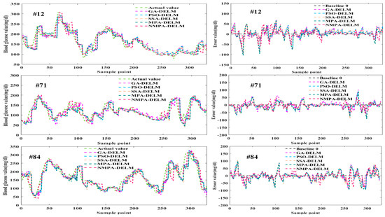
Figure 11.
Prediction results and error curves graphs of different patients.
As can be seen from Figure 10 and Figure 11, compared with other models, the predicted values of the NMPA-DELM model are closer to the actual values and have a smaller prediction error. In addition, the predicted values of area A in the CEGA diagram are the most in the NMPA-DELM model. The results show that compared with GA, PSO, SSA and MPA algorithms, the NMPA algorithm has the best optimization performance. It can improve the prediction performance and accuracy of the DELM model to the greatest extent, and has certain feasibility in blood glucose prediction.
4.5. Comparison Between VMD-TVF-EMD-NMPA-DELM Model Versus Other Hybrid Models
We compare the VMD-TVF-EMD-NMPA-DELM prediction model proposed in this paper with other hybrid prediction models to further verify its prediction performance. The VMD-TVF-EMD-NMPA-ELM, POA-TVF-EMD-CNN-LSTM-EC, CEEMDAN-SE-EC-BiLSTM, VMD-TVF-EMD-NMPA-LSTM and VMD-TVF-EMD-NMPA-DELM models are used to predict blood glucose concentrations 45 min in advance for different patients. For easier display, the first four models are referred to as model 1, model 2, model 3 and model 4. The performance indicators of each model are shown in Table 3.
Table 3.
Performance indicator results of all five models for all patients.
As can be seen from Table 3, the MAE, RMSE and MAPE values of the VMD-TVF-EMD-NMPA-DELM model are lower than those of the other four hybrid models. This shows that the prediction performance of the VMD-TVF-EMD-NMPA-DELM model is better than that of the other four hybrid models. Among the five models, the prediction accuracy of the VMD-TVF-EMD-NMPA-ELM model is the worst. Compared with the prediction results of the VMD-TVF-EMD-NMPA-ELM model, the MAE, RMSE and MAPE of the VMD-TVF-EMD-NMPA-ELM model are reduced by 0.9586, 1.0078 and 0.5882% at most, respectively. The results show that the VMD-TVF-EMD-NMPA-DELM model proposed in this paper shows obvious advantages in prediction accuracy and performance, and has a higher prediction ability than the other four hybrid models.
The results of all model performance indicators are drawn, and the CEGA diagram of each model is also included, as shown in Figure 12. Then, the blood glucose prediction results and error curve of each model 45 min in advance for different patients were drawn, as shown in Figure 13.
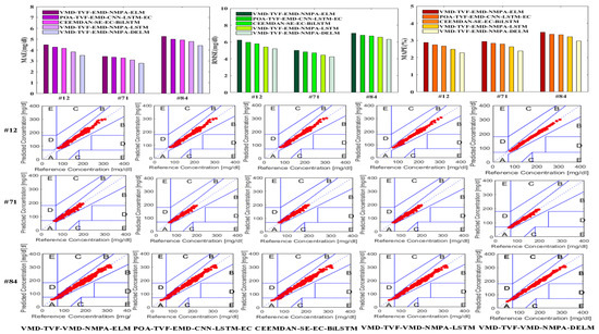
Figure 12.
Error performance index results and CEGA chart for each patient.
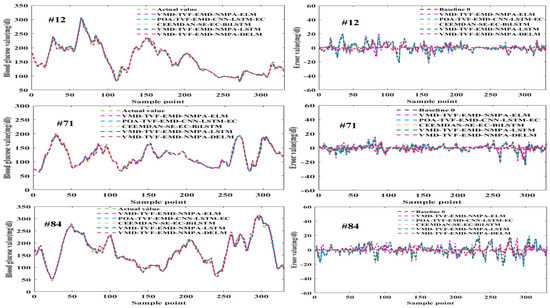
Figure 13.
Prediction results and error curves of five models.
From Figure 12 and Figure 13, it can be seen that the predicted values of the VMD-TVF-EMD-NMPA-DELM model proposed in this paper are highly consistent with the actual values, and that its prediction error and performance indicators are superior to those of the other four hybrid models. Meanwhile, in the CEGA graph, all predicted values of the VMD-TVF-EMD-NMPA-DELM model fall into region A, further demonstrating its superior predictive performance.
4.6. Statistical Robustness Analysis and Diebold–Mariano Test
In order to effectively improve the statistical robustness of the research results, 10 diabetes patients are added here for blood glucose prediction. Comparing and analyzing the error performance of 12 prediction models for predicting blood glucose concentration levels 45 min in advance for these patients, the performance indicators of MAE, RMSE and MAPE of different prediction methods are shown in Table 4.
Table 4.
Performance indicators of MAE, RMSE and MAPE for different methods.
From Table 4, it can be seen that, when predicted 45 min in advance, the MAE, RMSE and MAPE values of the NMPA-DELM prediction model are better than those of the DELM prediction model. The prediction results indicate that the NMPA-DELM model has better predictive ability than the DELM model. And, the predictive ability of this model is also superior to GA-DELM, PSO-DELM, SSA-DELM and MPA-DELM models, which fully demonstrates the advantages of NMPA algorithm in DELM network parameter optimization. By comparing the prediction results of NMPA-DELM and VMD-NMPA-DELM, it can be found that the VMD decomposition effectively improves the prediction accuracy of the model.
Comparing the prediction results of VMD-NMPA-DELM and VMD-TVF-EMD-NMPA-DELM, it can be seen that the predictive ability of the VMD-NMPA-DELM model has been further improved after TVF-EMD decomposition processing. Compared with the VMD-NMPA-DELM model, when predicted 45 min in advance, the MAE, RMSE and MAPE of the VMD-TVF-EMD-NMPA-DELM model decreased by 0.7157, 0.8944 and 0.4526%, respectively. Comparing the prediction results of the last five mixed models in Table 4, it can be found that the three performance indicators of the VMD-TVF-EMD-NMPA-DELM model proposed in this paper are still the best. This fully demonstrates the advantages of VMD-TVF-EMD-NMPA-DELM in predicting blood glucose concentration. By comparing the data in Table 4, it can be seen that the VMD-TVF-EMD-NMPA-DELM model has the smallest MAE, RMSE and MAPE among all models, indicating that the model proposed in this paper has the best predictive performance.
To further validate the superiority of the VMD-TVF-EMD-NMPA-DELM model proposed in this paper, the predictive performance of different models was evaluated through the Diebold Mariano (DM) test. The DM test is a statistical method used to compare the performance of two prediction models. Its main purpose is to determine whether there is a significant difference in the predictive ability of the two models by analyzing the prediction error. The results of the DM test are shown in Table 5.
Table 5.
The results of DM test.
The DM test statistics in Table 5 are all greater than 1.96, and the p-values are far less than 0.05. The results show that the VMD-TVF-EMD-NMPA-DELM model proposed in this article is significantly better than other comparison models in accuracy.
4.7. Real-Time Analysis
The experimental system environment is Windows 11, with a 2.50 GHz i5 processor and a memory capacity of 16.0 GB. The experimental software is the MATLAB 2021a version. The entire process is divided into two stages: training and execution. We calculate the time spent in these two stages. The running times of the different models are analyzed and discussed accordingly from the point of view of time complexity. The specific time consumption of each model is shown in Table 6 below.
Table 6.
Real-time results of different methods.
From the comparative analysis in Table 6, it can be seen that the various methods consume a certain amount of time in constructing the network, and the time required for training varies due to the differences in the network structure. According to Table 6, it can be found that the DELM model takes the shortest time when the network is in the training stage. The VMD-TVF-EMD-NMPA-LSTM method takes the longest time, about 358 s. The VMD-TVF-EMD-NMPA-DELM method proposed in this article takes no more than 102 s. When the network is in the execution stage, the VMD-TVF-EMD-NMPA-DELM method proposed in this paper only takes about 1.1 s. Compared with models without decomposition methods, the VMD-TVF-EMD-NMPA-DELM model has a longer computation time. This is understandable because the model has a stronger predictive ability. Compared to other hybrid models, the VMD-TVF-EMD-NMPA-DELM method proposed in this paper takes relatively less time. From this, it can be concluded that, in practical applications, except for the training phase at the beginning of program startup which requires approximately 102 s of waiting time, blood glucose concentration prediction results can be quickly provided during other time periods. Therefore, to a certain extent, the VMD-TVF-EMD-NMPA-DELM method proposed in this paper is sufficient to meet the real-time requirements.
5. Conclusions
Modern and effective techniques are used to improve the accuracy of blood glucose prediction in patients in order to achieve accurate control of blood glucose concentrations. This approach has important implications for reducing the risk of diabetes-related complications. It not only helps to improve the health of patients, but also reduces the psychological and living burden of their families. To attain high precision in blood glucose forecasting outcomes, a glucose forecasting model is introduced, leveraging the double decomposition strategy and NMPA algorithm-optimized DELM. First of all, in order to fully decrease the non-stationarity and nonlinearity of the original blood glucose data, the VMD method is employed to dismantle the initial blood glucose series and extract the residual component after treatment. Subsequently, the TVF-EMD method is applied to further decompose this component, ensuring thorough decomposition. Then, individual DELM models are constructed for each subsequence, leveraging the NMPA algorithm to adjust the weight parameters to further enhance the prediction performance of the network. Ultimately, the ultimate blood glucose forecasting is derived by overlaying the predicted outcomes of each subsequence. The model undergoes validation using distinct blood glucose data and the results are compared with those of eleven models. The key findings are summarized as follows: (1) The non-stationarity and complexity of the initial blood glucose data can be effectively reduced by the decomposition of VMD. The residual component generated after VMD processing contains the key information of the original blood glucose sequence. However, the variation of residual components is relatively complex. By using the TVF-EMD method to decompose the residual component, a more complete and effective decomposition effect can be achieved; (2) DELM has powerful nonlinear fitting capabilities, performs well in processing complex blood glucose concentration data, and can achieve better forecasting outcomes. By applying the NMPA method to refine the DELM weight parameters, the prediction accuracy can be effectively improved; (3) Compared with the results obtained from other eleven models, the model introduced in this study exhibits superior accuracy and applicability in predicting blood glucose; (4) The model introduced in this research not only effectively improves the forecasting accuracy, but also extends the overall prediction time. While achieving blood glucose prediction 45 min in advance, it can still accurately capture the patient’s blood sugar fluctuation trend.
The important direction of follow-up research is how to effectively reduce the time required for decomposing blood glucose data. Furthermore, future work can take into account different factors that affect the change of blood glucose fluctuations on the basis of this approach. Other effective signal decomposition techniques and optimization algorithms of DELM network parameters must be researched and developed.
Author Contributions
Conceptualization, Y.S.; writing—original draft, Y.S.; software, Y.S.; visualization, D.L.; data curation, D.L.; supervision, W.W.; writing—review and editing, W.W. and X.D.; project administration, X.D. All authors have read and agreed to the published version of the manuscript.
Funding
This work was supported by “the 14th Five Year Plan” Hubei Provincial advantaged characteristic disciplines (groups) project of Wuhan University of Science and Technology (2023C0204).
Data Availability Statement
The data that support the findings of this study are available from the corresponding author upon reasonable request.
Conflicts of Interest
The authors declare no conflicts of interest.
References
- Arora, S.; Kumar, S.; Kumar, P. Multivariate models of blood glucose prediction in type1 diabetes: A survey of the state-of-the-art. Curr. Pharm. Biotechnol. 2023, 24, 532–552. [Google Scholar] [PubMed]
- Wang, Y.; Wang, T. Application of improved LightGBM model in blood glucose prediction. Appl. Sci. 2020, 10, 3227. [Google Scholar] [CrossRef]
- Prendin, F.; Pavan, J.; Cappon, G.; Del Favero, S.; Sparacino, G.; Facchinetti, A. The importance of interpreting machine learning models for blood glucose prediction in diabetes: An analysis using SHAP. Sci. Rep. 2023, 13, 16865. [Google Scholar] [CrossRef] [PubMed]
- Zhu, T.; Wang, W.; Yu, M. A novel blood glucose time series prediction framework based on a novel signal decomposition method. Chaos Solitons Fractals 2022, 164, 112673. [Google Scholar] [CrossRef]
- Lu, H.Y.; Ding, X.; Hirst, J.E.; Yang, Y.; Yang, J.; Mackillop, L.; Clifton, D.A. Digital health and machine learning technologies for blood glucose monitoring and management of gestational diabetes. IEEE Rev. Biomed. Eng. 2023, 17, 98–117. [Google Scholar] [CrossRef]
- Xie, J.; Wang, Q. Benchmarking machine learning algorithms on blood glucose prediction for type I diabetes in comparison with classical time-series models. IEEE Trans. Biomed. Eng. 2020, 67, 3101–3124. [Google Scholar] [CrossRef]
- Sevil, M.; Rashid, M.; Hajizadeh, I.; Park, M.; Quinn, L.; Cinar, A. Physical activity and psychological stress detection and assessment of their effects on glucose concentration predictions in diabetes management. IEEE Trans. Biomed. Eng. 2021, 68, 2251–2260. [Google Scholar] [CrossRef]
- Rabby, M.F.; Tu, Y.; Hossen, M.I.; Lee, I.; Maida, A.S.; Hei, X. Stacked LSTM based deep recurrent neural network with kalman smoothing for blood glucose prediction. BMC Med. Inform. Decis. Mak. 2021, 21, 101. [Google Scholar] [CrossRef]
- Alfian, G.; Syafrudin, M.; Anshari, M.; Benes, F.; Atmaji, F.T.D.; Fahrurrozi, I.; Hidayatullah, A.F.; Rhee, J. Blood glucose prediction model for type 1 diabetes based on artificial neural network with time-domain features. Biocybern. Biomed. Eng. 2020, 40, 1586–1599. [Google Scholar] [CrossRef]
- Li, N.; Tuo, J.; Wang, Y.; Wang, M. Prediction of blood glucose concentration for type 1 diabetes based on echo state networks embedded with incremental learning. Neurocomputing 2020, 378, 248–259. [Google Scholar] [CrossRef]
- Iacono, F.; Magni, L.; Toffanin, C. Personalized LSTM-based alarm systems for hypoglycemia and hyperglycemia prevention. Biomed. Signal Process. Control 2023, 86, 105167. [Google Scholar] [CrossRef]
- Jaloli, M.; Cescon, M. Long-term prediction of blood glucose levels in type 1 diabetes using a CNN-LSTM-based deep neural network. J. Diabetes Sci. Technol. 2023, 17, 1590–1601. [Google Scholar] [CrossRef] [PubMed]
- Dudukcu, H.V.; Taskiran, M.; Yildirim, T. Blood glucose prediction with deep neural networks using weighted decision level fusion. Biocybern. Biomed. Eng. 2021, 41, 1208–1223. [Google Scholar] [CrossRef]
- Saravanan, R.; Mahmud, F. Blood Glucose Prediction Based on ARIMA Time-Series Machine Learning Model. Evol. Electr. Electron. Eng. 2023, 4, 457–463. [Google Scholar]
- Ding, S.; Zhao, H.; Zhang, Y.; Xu, X.; Nie, R. Extreme learning machine: Algorithm, theory and applications. Artif. Intell. Rev. 2015, 44, 103–115. [Google Scholar] [CrossRef]
- Daniels, J.; Herrero, P.; Georgiou, P. A multitask learning approach to personalized blood glucose prediction. IEEE J. Biomed. Health Inform. 2021, 26, 436–445. [Google Scholar] [CrossRef]
- Martinsson, J.; Schliep, A.; Eliasson, B.; Mogren, O. Blood glucose prediction with variance estimation using recurrent neural networks. J. Healthc. Inform. Res. 2020, 4, 1–18. [Google Scholar] [CrossRef]
- Wang, W.; Tong, M.; Yu, M. Blood glucose prediction with VMD and LSTM optimized by improved particle swarm optimization. IEEE Access 2020, 8, 217908–217916. [Google Scholar] [CrossRef]
- Yang, T.; Yu, X.; Ma, N.; Wu, R.; Li, H. An autonomous channel deep learning framework for blood glucose prediction. Appl. Soft Comput. 2022, 120, 108636. [Google Scholar] [CrossRef]
- Zhu, T.; Li, K.; Chen, J.; Herrero, P.; Georgiou, P. Dilated recurrent neural networks for glucose forecasting in type 1 diabetes. J. Healthc. Inform. Res. 2020, 4, 308–324. [Google Scholar] [CrossRef]
- Yang, G.; Liu, S.; Li, Y.; He, L. Short-term prediction method of blood glucose based on temporal multi-head attention mechanism for diabetic patients. Biomed. Signal Process. Control 2023, 82, 104552. [Google Scholar] [CrossRef]
- Kumari, G.L.A.; Padmaja, P.; Suma, J.G. A novel method for prediction of diabetes mellitus using deep convolutional neural network and long short-term memory. Indones. J. Electr. Eng. Comput. Sci. 2022, 26, 404–413. [Google Scholar] [CrossRef]
- Long, X.; Wang, J.; Gong, S.; Li, G.; Ju, H. Reference evapotranspiration estimation using long short-term memory network and wavelet-coupled long short-term memory network. Irrig. Drain. 2022, 71, 855–881. [Google Scholar] [CrossRef]
- Meng, A.; Zhu, Z.; Deng, W.; Ou, Z.; Lin, S.; Wang, C.; Xu, X.; Wang, X.; Yin, H.; Luo, J. A novel wind power prediction approach using multivariate variational mode decomposition and multi-objective crisscross optimization based deep extreme learning machine. Energy 2022, 260, 124957. [Google Scholar] [CrossRef]
- Siddiqui, S.Y.; Khan, M.A.; Abbas, S.; Khan, F. Smart occupancy detection for road traffic parking using deep extreme learning machine. J. King Saud Univ. Comput. Inf. Sci. 2022, 34, 727–733. [Google Scholar]
- Xiong, J.; Liang, W.; Liang, X.; Yao, J. Intelligent quantification of natural gas pipeline defects using improved sparrow search algorithm and deep extreme learning machine. Chem. Eng. Res. Des. 2022, 183, 567–579. [Google Scholar] [CrossRef]
- Song, C.; Yao, L. Application of artificial intelligence based on synchrosqueezed wavelet transform and improved deep extreme learning machine in water quality prediction. Environ. Sci. Pollut. Res. 2022, 29, 38066–38082. [Google Scholar] [CrossRef]
- Sadiq, A.S.; Dehkordi, A.A.; Mirjalili, S.; Pham, Q.V. Nonlinear marine predator algorithm: A cost-effective optimizer for fair power allocation in NOMA-VLC-B5G networks. Expert Syst. Appl. 2022, 203, 117395. [Google Scholar] [CrossRef]
- Garai, S.; Paul, R.K.; Yeasin, M.; Paul, A.K. CEEMDAN-Based Hybrid Machine Learning Models for Time Series Forecasting Using MARS Algorithm and PSO-Optimization. Neural Process. Lett. 2024, 56, 92. [Google Scholar] [CrossRef]
- Jian, X.; Xia, Y.; Sun, L. An indirect method for bridge mode shapes identification based on wavelet analysis. Struct. Control Health Monit. 2020, 27, e2630. [Google Scholar] [CrossRef]
- Zhang, Y.; Li, C.; Jiang, Y.; Sun, L.; Zhao, R.; Yan, K.; Wang, W. Accurate prediction of water quality in urban drainage network with integrated EMD-LSTM model. J. Clean. Prod. 2022, 354, 131724. [Google Scholar] [CrossRef]
- Zuo, G.; Luo, J.; Wang, N.; Lian, Y.; He, X. Decomposition ensemble model based on variational mode decomposition and long short-term memory for streamflow forecasting. J. Hydrol. 2020, 585, 124776. [Google Scholar] [CrossRef]
- Gu, J.; Peng, Y.; Lu, H.; Chang, X.; Cao, S.; Chen, G.; Cao, B. An optimized variational mode decomposition method and its application in vibration signal analysis of bearings. Struct. Health Monit. 2022, 21, 2386–2407. [Google Scholar] [CrossRef]
- Gan, M.; Pan, H.; Chen, Y.; Pan, S. Application of the Variational Mode Decomposition (VMD) method to river tides. Estuar. Coast. Shelf Sci. 2021, 261, 107570. [Google Scholar] [CrossRef]
- Li, H.; Li, Z.; Mo, W. A time varying filter approach for empirical mode decomposition. Signal Process. 2017, 138, 146–158. [Google Scholar] [CrossRef]
- Rehman, A.; Athar, A.; Khan, M.A.; Abbas, S.; Fatima, A.; Saeed, A. Modelling, simulation, and optimization of diabetes type II prediction using deep extreme learning machine. J. Ambient Intell. Smart Environ. 2020, 12, 125–138. [Google Scholar] [CrossRef]
- Faramarzi, A.; Heidarinejad, M.; Mirjalili, S.; Gandomi, A.H. Marine Predators Algorithm: A nature-inspired metaheuristic. Expert Syst. Appl. 2020, 152, 113377. [Google Scholar] [CrossRef]
- Wang, W.; Shen, Y.; Chen, G. Blood glucose concentration prediction based on VMD-KELM-AdaBoost. Med. Biol. Eng. Comput. 2021, 59, 2219–2235. [Google Scholar]
- Ding, L.; Bai, Y.; Liu, M.D.; Fan, M.H.; Yang, J. Predicting short wind speed with a hybrid model based on a piecewise error correction method and Elman neural network. Energy 2022, 244, 122630. [Google Scholar] [CrossRef]
- Noorollahi, Y.; Jokar, M.A.; Kalhor, A. Using artificial neural networks for temporal and spatial wind speed forecasting in Iran. Energy Convers. Manag. 2016, 115, 17–25. [Google Scholar] [CrossRef]
Disclaimer/Publisher’s Note: The statements, opinions and data contained in all publications are solely those of the individual author(s) and contributor(s) and not of MDPI and/or the editor(s). MDPI and/or the editor(s) disclaim responsibility for any injury to people or property resulting from any ideas, methods, instructions or products referred to in the content. |
© 2024 by the authors. Licensee MDPI, Basel, Switzerland. This article is an open access article distributed under the terms and conditions of the Creative Commons Attribution (CC BY) license (https://creativecommons.org/licenses/by/4.0/).