New Abundant Analytical Solitons to the Fractional Mathematical Physics Model via Three Distinct Schemes

Abstract

New types of truncated M-fractional wave solitons to the simplified Modified Camassa–Holm model, a mathematical physics model, are obtained. This model is used to explain the unidirectional propagation of shallow water waves. The required solutions are obtained by utilizing the simplest equation, the Sardar subequation, and the generalized Kudryashov schemes. The obtained results consist of the dark, singular, periodic, dark-bright, and many other analytical solitons. Dynamical behaviors of some obtained solutions are represented by two-dimensional (2D), three-dimensional (3D), and Contour graphs. An effect of fractional derivative is shown graphically. The results are newer than the existing results of the governing equation. Obtained solutions have much importance in the various areas of applied science as well as engineering. We concluded that the utilized methods are helpful and applicable for other partial fractional equations in applied science and engineering.

1. Introduction

Soliton theory, which originated in the sixties and seventies of the past century, has played a crucial rule in many areas, including plasmas and optical fibers. It has much importance in applied mathematics with various applications in optical fibers, ferromagnetic dynamics, optics, etc. The applications of this theory extend its influence across a wide spectrum of natural sciences, such as telecommunication, engineering, etc. In modern days, phenomena that occur in nature are represented as fractional nonlinear partial differential Equations (FNLPDEs) [1,2].

Obtaining exact solutions to NLPDEs is achieved via various techniques, which encompass methods such as the modified direct algebraic technique [3], the modified Khater scheme [4], the Kudryashov technique [5], novel $(G^{\prime }/G)$-expansion technique [6], extended FAN subequation technique [7,8] and extended mapping scheme [9], the ${\partial }^{-}$-dressing technique [10], Riemann–Hilbert approach [11], the ${\partial }^{-}$-generalized Deift–Zhou nonlinear steepest descent method [12], extended $(G^{\prime }/G)$-expansion technique [13], extended Sinh-Gordon expansion technique [14], modified extended tanh function method [15], Hirota method [16], and generalized Eigenfunction technique [17].

In this research, we consider three simple yet useful methods: the modified simplest equation technique, the Sardar subequation technique, and the generalized Kudryashov technique. Different kinds of models are solved by using these techniques. Modified simplest equation techniques are employed to derive exact solitons of coupled Higgs equation, with Maccari’s model in [18], different solitary wave solitons of Gardner model in [19], and optical soliton solutions of the Radha–Lakshmanan equation in [20]. The Sardar subequation technique has been utilized to obtain the many kinds of wave solitons for the Sawada–Kotera (SK) equation [21], optical solitons for the Fokas–Lenells equation were achieved in [22], and some new kinds of exact soliton solutions for the nonlinear Akbota equation were obtained in [23]. Similarly, the generalized Kudryashov scheme has been instrumental in finding various types of wave solutions, including the bell, dark, kink, and others for the Fokas–Lenelles equation [24], exact solitons for the KdV-Burger model [25], and some general solutions for the Kolmogorov–Petrovskii–Piskunov Equation [26], among other applications.

Our primary mathematical physics model is the nonlinear simplified Modified Camassa–Holm model (SMCHM). Various techniques have been employed to derive different types of exact solitons for this model. The generalized $(G^{\prime }/G)$-expansion technique was used to derive specific types of traveling wave solitons in [27], while the Exp-function technique yielded solitary wave solitons in [28]. Moreover, other forms of exact solutions were obtained by utilizing the Riccati–Bernoulli sub-ODE scheme in [29], while some new kinds of soliton solutions, including the smooth kink, flat kink, and singular periodic kink, were gained by using the extended Kudryashov technique in [30], and different soliton solutions, including the bell-shaped, anti-bell shaped, compacton, and singular bell-shaped solitons, were obtained by applying the $(G^{\prime }/G,1/G)$-expansion method in [31], among many others.

The purpose of this research is to explore novel types of exact wave solitons to the (1+1)-D simplified Modified Camassa–Holm model by using three distinct techniques: the modified simplest equation, the Sardar subequation, and the generalized Kudryashov technique.

This paper is organized into several sections. Section 2 gives an explanation of the equation and its mathematical treatment. In Section 3, we give the details of the modified simplest equation scheme and its use in obtaining wave solitons. Section 4 focuses on the Sardar subequation scheme and its implementation to derive new wave solitons. Section 5 delves into the generalized Kudryashov scheme and its implementation in obtaining wave solutions. In Section 6, we showcase some of the derived results by two-dimensional, three-dimensional, and contour plots. Finally, we present our conclusions in Section 7.

2. The Concerning Equation and Its Mathematical Treatment

The simplified modified Camassa–Holm (SMCH) equation is a nonlinear model that is important for understanding and classifying wave phenomena in ocean engineering and science. The equation is used to model the propagation of shallow water waves that are characterized by nonlinearities and weak dispersion. The simplified MCH, a developed Korteweg–de Vries equation, is an integrable nonlinear dispersive water wave equation with potential applications in diverse fields, such as shallow water waves, liquid drop patterning, water surface waves in channels, tsunamis in coastal regions, oceans, etc. Assume a nonlinear truncated M-fractional simplified modified Camassa–Holm model, which belong to the class of significant equations known as modified $\beta$-equations, as described by Wazwaz [32]:

$$D_{M,t}^{\alpha ,\gamma }g-D_{M,t}^{\alpha ,\gamma }(D_{M,2x}^{2\alpha ,\gamma }g)+(\beta +1)g^2{D}_{M,2x}^{2\alpha ,\gamma }g-\beta D_{M,x}^{\alpha ,\gamma }g{D}_{M,2x}^{2\alpha ,\gamma }g-D_{M,3x}^{3\alpha ,\gamma }g=0.\beta >0.$$

(1)

where $g=g(x,t)$ shows a wave-profile where $\Omega$ and $\theta$ are nonzero parameters. Substituting $\beta =2$ into Equation (1) implies:

$$D_{M,t}^{\alpha ,\gamma }g-D_{M,t}^{\alpha ,\gamma }(D_{M,2x}^{2\alpha ,\gamma }g)+3g^2{D}_{M,2x}^{2\alpha ,\gamma }g-2D_{M,x}^{\alpha ,\gamma }g{D}_{M,2x}^{2\alpha ,\gamma }g-D_{M,3x}^{3\alpha ,\gamma }g=0.$$

(2)

Equation (2) is called the modified Camassa–Holm model. A more simplified form of Equation (2) is shown by [33]:

$$D_{M,t}^{\alpha ,\gamma }g+2\Omega D_{M,x}^{\alpha ,\gamma }g-D_{M,t}^{\alpha ,\gamma }(D_{M,2x}^{2\alpha ,\gamma }g)+\theta g^2{D}_{M,x}^{\alpha ,\gamma }g=0.\Omega \in \Re \beta >0$$

(3)

where

$$D_{M,t}^{\alpha ,{\rm Y}}g(t)=\underset{\tau \to 0}{lim}{\displaystyle \frac{g(t{E}_{{\rm Y}}(\tau t^{1-\alpha }))-g(t)}{\tau }},\alpha \in (0,1],{\rm Y}>0,$$

(4)

in which $E_{{\rm Y}}(.)$ indicates a truncated Mittag–Leffler (ML) profile [34,35].

Consider the following wave transformation:

$$g(x,t)=G(\xi ),\xi ={\displaystyle \frac{1}{\alpha }}\Gamma ({\rm Y}+1)(\mu x^{\alpha }+\delta t^{\alpha }),$$

(5)

Here, $\mu$, and $\delta$ are the constants. Putting Equation (5) in Equation (3), we attain

$$(\delta +2\Omega \mu )G-\delta {\mu }^2{G}^{\prime \prime }+{\displaystyle \frac{\theta \mu }{3}}{G}^3=0.$$

(6)

3. Modified Simplest Equation Technique

Here, there is a basic concept of this scheme given as follows:

• Step 1: Suppose a nonlinear partial differential equation:

  $$Y(g,g^2,g^2{g}_x,g_{xx},g_{xt},\dots )=0,$$

  (7)

  where $g=g(x,t)$ denotes a real wave-profile. Suppose the given relation:

  $$g(x,t)=G(\Theta ),\Theta =x+\lambda t.$$

  (8)
  Inserting Equation (8) in Equation (7), a nonlinear ordinary differential equation is obtained

  $$Z(G,G^2{G}^{\prime },G^{″},...)=0.$$

  (9)
• Step 2: Consider Equation (9) has solution given as:

  $$G(\Theta )=\sum _{s=1}^m{b}_s{\varphi }^s(\Theta ),$$

  (10)

  where $b_s(s=1,2,3,...,m)$ represent the undetermined. A novel profile $\varphi (\Theta )$ satisfies the ODE:

  $${\varphi }^{\prime }(\Theta )={\varphi }^2(\Theta )+\mho ,$$

  (11)

  where ℧ indicates a constant. Notice that Equation (11) has the distinct results based on ℧:
  If $\mho <0$, then:

  $$\varphi (\Theta )=-\sqrt{-\mho }tanh(\sqrt{-\mho }\Theta ),$$

  (12)

  $$\varphi (\Theta )=-\sqrt{-\mho }coth(\sqrt{-\mho }\Theta ),$$

  (13)

  $$\varphi (\Theta )=\sqrt{-\mho }(-tanh(2\sqrt{-\mho }\Theta )\pm isech(2\sqrt{-\mho }\Theta )),$$

  (14)

  $$\varphi (\Theta )=\sqrt{-\mho }(-coth(2\sqrt{-\mho }\Theta )\pm csch(2\sqrt{-\mho }\Theta )),$$

  (15)

  $$\varphi (\Theta )=-{\displaystyle \frac{\sqrt{-\mho }}{2}}(tanh({\displaystyle \frac{\sqrt{-\mho }}{2}}\Theta )+coth({\displaystyle \frac{\sqrt{-\mho }}{2}}\Theta )).$$

  (16)
  If $\mho >0$:

  $$\varphi (\Theta )=\sqrt{\mho }tan(\sqrt{\mho }\Theta ),$$

  (17)

  $$\varphi (\Theta )=-\sqrt{\mho }cot(\sqrt{\mho }\Theta ),$$

  (18)

  $$\varphi (\Theta )=\sqrt{\mho }(tan(2\sqrt{\mho }\Theta )\pm sec(2\sqrt{\mho }\Theta )),$$

  (19)

  $$\varphi (\Theta )=\sqrt{\mho }(-cot(2\sqrt{\mho }\Theta )\pm csc(2\sqrt{\mho }\Theta )),$$

  (20)

  $$\varphi (\Theta )={\displaystyle \frac{\sqrt{\mho }}{2}}(tan({\displaystyle \frac{\sqrt{\mho }}{2}}\Theta )-cot({\displaystyle \frac{\sqrt{\mho }}{2}}\Theta )).$$

  (21)
  If $\mho =0$,

  $$\varphi (\Theta )=-{\displaystyle \frac{1}{\Theta }}.$$

  (22)
• Step 3: Using Equation (10) and Equation (11) in Equation (9). Summing up the coefficients of every ${\varphi }^j$, taking the coefficients of same order equal to 0 to obtain a system involving $b_s$ and $\lambda$. By solving the system, solutions for the undetermined are obtained.

Step 4: Putting Equation (9), where $b_s$ and $\lambda$ are obtained in Equation (10) will result in Equation (7).

Application of MSE Scheme

Equation (10) changes into the given form in our case:

$$G(\xi )=b_0+b_1\psi (\xi ).$$

(23)

Using Equation (23) and Equation (11) in Equation (6), one obtains the given sets. Set 1:

$$\left\{b_0=0,b_1=-{\displaystyle \frac{2\sqrt{3}\mu \sqrt{\Omega }}{\sqrt{2\theta {\mu }^2\mho -\theta }}},\delta ={\displaystyle \frac{2\mu \Omega }{2{\mu }^2\mho -1}}\right\}.$$

(24)

Case 1: if $\mho <0$:

$$g(x,t)=-{\displaystyle \frac{2\sqrt{3}\mu \sqrt{\Omega }}{\sqrt{2\theta {\mu }^2\mho -\theta }}}(-\sqrt{-\mho }tanh(\sqrt{-\mho }{\displaystyle \frac{1}{\alpha }}\Gamma (1+{\rm Y})(\mu x^{\alpha }+({\displaystyle \frac{2\mu \Omega }{2{\mu }^2\mho -1}})t^{\alpha }))).$$

(25)

$$g(x,t)=-{\displaystyle \frac{2\sqrt{3}\mu \sqrt{\Omega }}{\sqrt{2\theta {\mu }^2\mho -\theta }}}(-\sqrt{-\mho }coth(\sqrt{-\mho }{\displaystyle \frac{\Gamma (1+{\rm Y})}{\alpha }}(\mu x^{\alpha }+({\displaystyle \frac{2\mu \Omega }{2{\mu }^2\mho -1}})t^{\alpha }))).$$

(26)

$$\begin{array}{c}g(x,t)=-{\displaystyle \frac{2\sqrt{3}\mu \sqrt{\Omega }}{\sqrt{2\theta {\mu }^2\mho -\theta }}}(\sqrt{-\mho }(-tanh(2\sqrt{-\mho }{\displaystyle \frac{\Gamma (1+{\rm Y})}{\alpha }}(\mu x^{\alpha }+({\displaystyle \frac{2\mu \Omega }{2{\mu }^2\mho -1}})t^{\alpha }))\hspace{1em}\hfill \\ \hfill \pm isech(2\sqrt{-\mho }{\displaystyle \frac{\Gamma (1+{\rm Y})}{\alpha }}(\mu x^{\alpha }+({\displaystyle \frac{2\mu \Omega }{2{\mu }^2\mho -1}})t^{\alpha })))).\end{array}$$

(27)

$$\begin{array}{c}g(x,t)=-{\displaystyle \frac{2\sqrt{3}\mu \sqrt{\Omega }}{\sqrt{2\theta {\mu }^2\mho -\theta }}}(\sqrt{-\mho }(-coth(2\sqrt{-\mho }{\displaystyle \frac{1}{\alpha }}\Gamma (1+{\rm Y})(\mu x^{\alpha }+({\displaystyle \frac{2\mu \Omega }{2{\mu }^2\mho -1}})t^{\alpha }))\hfill \\ \hfill \pm csch(2\sqrt{-\mho }{\displaystyle \frac{\Gamma (1+{\rm Y})}{\alpha }}(\mu x^{\alpha }+({\displaystyle \frac{2\mu \Omega }{2{\mu }^2\mho -1}})t^{\alpha })))).\end{array}$$

(28)

$$\begin{array}{c}g(x,t)=-{\displaystyle \frac{2\sqrt{3}\mu \sqrt{\Omega }}{\sqrt{2\theta {\mu }^2\mho -\theta }}}(-{\displaystyle \frac{\sqrt{-\mho }}{2}}(tanh({\displaystyle \frac{\sqrt{-\mho }}{2}}{\displaystyle \frac{\Gamma (1+{\rm Y})}{\alpha }}(\mu x^{\alpha }+({\displaystyle \frac{2\mu \Omega }{2{\mu }^2\mho -1}})t^{\alpha }))\hspace{1em}\hfill \\ \hfill +coth({\displaystyle \frac{\sqrt{-\mho }}{2}}{\displaystyle \frac{1}{\alpha }}\Gamma (1+{\rm Y})(\mu x^{\alpha }+({\displaystyle \frac{2\mu \Omega }{2{\mu }^2\omega -1}})t^{\alpha })))).\end{array}$$

(29)

Case 2: if $\mho >0$:

$$g(x,t)=-{\displaystyle \frac{2\sqrt{3}\mu \sqrt{\Omega }}{\sqrt{2\theta {\mu }^2\mho -\theta }}}(\sqrt{\mho }tan(\sqrt{\mho }{\displaystyle \frac{\Gamma (1+{\rm Y})}{\alpha }}(\mu x^{\alpha }+({\displaystyle \frac{2\mu \Omega }{2{\mu }^2\mho -1}})t^{\alpha }))).$$

(30)

$$g(x,t)=-{\displaystyle \frac{2\sqrt{3}\mu \sqrt{\Omega }}{\sqrt{2\theta {\mu }^2\mho -\theta }}}(-\sqrt{\mho }cot(\sqrt{\mho }{\displaystyle \frac{\Gamma (1+{\rm Y})}{\alpha }}(\mu x^{\alpha }+({\displaystyle \frac{2\mu \Omega }{2{\mu }^2\mho -1}})t^{\alpha }))).$$

(31)

$$\begin{array}{c}g(x,t)=-{\displaystyle \frac{2\sqrt{3}\mu \sqrt{\Omega }}{\sqrt{2\theta {\mu }^2\mho -\theta }}}(\sqrt{\mho }(tan(2\sqrt{\mho }{\displaystyle \frac{\Gamma (1+{\rm Y})}{\alpha }}(\mu x^{\alpha }+({\displaystyle \frac{2\mu \Omega }{2{\mu }^2\mho -1}})t^{\alpha }))\hspace{1em}\hspace{1em}\hspace{1em}\hspace{1em} \hfill \\ \hfill \pm sec(2\sqrt{\mho }{\displaystyle \frac{\Gamma (1+{\rm Y})}{\alpha }}(\mu x^{\alpha }+({\displaystyle \frac{2\mu \Omega }{2{\mu }^2\mho -1}})t^{\alpha })))).\end{array}$$

(32)

$$\begin{array}{c}g(x,t)=-{\displaystyle \frac{2\sqrt{3}\mu \sqrt{\Omega }}{\sqrt{2\theta {\mu }^2\mho -\theta }}}(\sqrt{\mho }(-cot(2\sqrt{\mho }{\displaystyle \frac{\Gamma (1+{\rm Y})}{\alpha }}(\mu x^{\alpha }+({\displaystyle \frac{2\mu \Omega }{2{\mu }^2\mho -1}})t^{\alpha }))\hspace{1em}\hspace{1em}\hspace{1em}\hspace{1em}\hfill \\ \hfill \pm csc(2\sqrt{\mho }{\displaystyle \frac{\Gamma (1+{\rm Y})}{\alpha }}(\mu x^{\alpha }+({\displaystyle \frac{2\mu \Omega }{2{\mu }^2\mho -1}})t^{\alpha })))).\end{array}$$

(33)

$$\begin{array}{c}g(x,t)=-{\displaystyle \frac{2\sqrt{3}\mu \sqrt{\Omega }}{\sqrt{2\theta {\mu }^2\mho -\theta }}}({\displaystyle \frac{\sqrt{\mho }}{2}}(tan({\displaystyle \frac{\sqrt{\mho }}{2}}{\displaystyle \frac{1}{\alpha }}\Gamma (1+{\rm Y})(\mu x^{\alpha }+({\displaystyle \frac{2\mu \Omega }{2{\mu }^2\mho -1}})t^{\alpha }))\hspace{1em}\hspace{1em}\hspace{1em} \hfill \\ \hfill -cot({\displaystyle \frac{\sqrt{\mho }}{2}}{\displaystyle \frac{\Gamma (1+{\rm Y})}{\alpha }}(\mu x^{\alpha }+({\displaystyle \frac{2\mu \Omega }{2{\mu }^2\mho -1}})t^{\alpha })))).\end{array}$$

(34)

Case 3: if $\mho =0$:

$$g(x,t)={\displaystyle \frac{2\sqrt{3}\mu \sqrt{\Omega }}{\sqrt{-\theta }\frac{\Gamma (1+{\rm Y})}{\alpha }(\mu x^{\alpha }-2\mu \Omega t^{\alpha })}}.$$

(35)

Set 2:

$$\left\{b_0=0,b_1={\displaystyle \frac{2\sqrt{3}\mu \sqrt{\Omega }}{\sqrt{2\theta {\mu }^2\mho -\theta }}},\delta ={\displaystyle \frac{2\mu \Omega }{2{\mu }^2\mho -1}}\right\}.$$

(36)

Case 1:if $\mho <0$:

$$g(x,t)={\displaystyle \frac{2\sqrt{3}\mu \sqrt{\Omega }}{\sqrt{2\theta {\mu }^2\mho -\theta }}}(-\sqrt{-\mho }tanh(\sqrt{-\mho }{\displaystyle \frac{1}{\alpha }}\Gamma (1+{\rm Y})(\mu x^{\alpha }+({\displaystyle \frac{2\mu \Omega }{2{\mu }^2\mho -1}})t^{\alpha }))).$$

(37)

$$g(x,t)={\displaystyle \frac{2\sqrt{3}\mu \sqrt{\Omega }}{\sqrt{2\theta {\mu }^2\mho -\theta }}}(-\sqrt{-\mho }coth(\sqrt{-\mho }{\displaystyle \frac{\Gamma (1+{\rm Y})}{\alpha }}(\mu x^{\alpha }+({\displaystyle \frac{2\mu \Omega }{2{\mu }^2\mho -1}})t^{\alpha }))).$$

(38)

$$\begin{array}{c}g(x,t)={\displaystyle \frac{2\sqrt{3}\mu \sqrt{\Omega }}{\sqrt{2\theta {\mu }^2\mho -\theta }}}(\sqrt{-\mho }(-tanh(2\sqrt{-\mho }{\displaystyle \frac{1}{\alpha }}\Gamma (1+{\rm Y})(\mu x^{\alpha }+({\displaystyle \frac{2\mu \Omega }{2{\mu }^2\mho -1}})t^{\alpha }))\hspace{1em}\hfill \\ \hfill \pm isech(2\sqrt{-\mho }{\displaystyle \frac{1}{\alpha }}\Gamma (1+{\rm Y})(\mu x^{\alpha }+({\displaystyle \frac{2\mu \Omega }{2{\mu }^2\mho -1}})t^{\alpha })))).\end{array}$$

(39)

$$\begin{array}{c}g(x,t)={\displaystyle \frac{2\sqrt{3}\mu \sqrt{\Omega }}{\sqrt{2\theta {\mu }^2\mho -\theta }}}(\sqrt{-\mho }(-coth(2\sqrt{-\mho }{\displaystyle \frac{1}{\alpha }}\Gamma (1+{\rm Y})(\mu x^{\alpha }+({\displaystyle \frac{2\mu \Omega }{2{\mu }^2\mho -1}})t^{\alpha }))\hspace{1em}\hfill \\ \hfill \pm csch(2\sqrt{-\mho }{\displaystyle \frac{\Gamma (1+{\rm Y})}{\alpha }}(\mu x^{\alpha }+({\displaystyle \frac{2\mu \Omega }{2{\mu }^2\mho -1}})t^{\alpha })))).\end{array}$$

(40)

$$\begin{array}{c}g(x,t)={\displaystyle \frac{2\sqrt{3}\mu \sqrt{\Omega }}{\sqrt{2\theta {\mu }^2\mho -\theta }}}(-{\displaystyle \frac{\sqrt{-\mho }}{2}}(tanh({\displaystyle \frac{\sqrt{-\mho }}{2}}{\displaystyle \frac{\Gamma (1+{\rm Y})}{\alpha }}(\mu x^{\alpha }+({\displaystyle \frac{2\mu \Omega }{2{\mu }^2\mho -1}})t^{\alpha }))\hspace{1em}\hspace{1em}\hfill \\ \hfill +coth({\displaystyle \frac{\sqrt{-\mho }}{2}}{\displaystyle \frac{\Gamma (1+{\rm Y})}{\alpha }}(\mu x^{\alpha }+({\displaystyle \frac{2\mu \Omega }{2{\mu }^2\mho -1}})t^{\alpha })))).\end{array}$$

(41)

Case 2: if $\mho >0$:

$$g(x,t)={\displaystyle \frac{2\sqrt{3}\mu \sqrt{\Omega }}{\sqrt{2\theta {\mu }^2\mho -\theta }}}(\sqrt{\mho }tan(\sqrt{\mho }{\displaystyle \frac{\Gamma (1+{\rm Y})}{\alpha }}(\mu x^{\alpha }+({\displaystyle \frac{2\mu \Omega }{2{\mu }^2\mho -1}})t^{\alpha }))).$$

(42)

$$g(x,t)={\displaystyle \frac{2\sqrt{3}\mu \sqrt{\Omega }}{\sqrt{2\theta {\mu }^2\mho -\theta }}}(-\sqrt{\mho }cot(\sqrt{\omega }{\displaystyle \frac{\Gamma (1+{\rm Y})}{\alpha }}(\mu x^{\alpha }+({\displaystyle \frac{2\mu \Omega }{2{\mu }^2\mho -1}})t^{\alpha }))).$$

(43)

$$\begin{array}{c}g(x,t)={\displaystyle \frac{2\sqrt{3}\mu \sqrt{\Omega }}{\sqrt{2\theta {\mu }^2\mho -\theta }}}(\sqrt{\mho }(tan(2\sqrt{\mho }{\displaystyle \frac{\Gamma (1+{\rm Y})}{\alpha }}(\mu x^{\alpha }+({\displaystyle \frac{2\mu \Omega }{2{\mu }^2\mho -1}})t^{\alpha }))\hspace{1em}\hspace{1em}\hspace{1em}\hspace{1em} \hspace{1em}\hfill \\ \hfill \pm sec(2\sqrt{\mho }{\displaystyle \frac{\Gamma (1+{\rm Y})}{\alpha }}(\mu x^{\alpha }+({\displaystyle \frac{2\mu \Omega }{2{\mu }^2\mho -1}})t^{\alpha })))).\end{array}$$

(44)

$$\begin{array}{c}g(x,t)={\displaystyle \frac{2\sqrt{3}\mu \sqrt{\Omega }}{\sqrt{2\theta {\mu }^2\mho -\theta }}}(\sqrt{\omega }(-cot(2\sqrt{\mho }{\displaystyle \frac{\Gamma (1+{\rm Y})}{\alpha }}(\mu x^{\alpha }+({\displaystyle \frac{2\mu \Omega }{2{\mu }^2\mho -1}})t^{\alpha }))\hspace{1em}\hspace{1em}\hspace{1em} \hspace{1em}\hfill \\ \hfill \pm csc(2\sqrt{\mho }{\displaystyle \frac{\Gamma (1+{\rm Y})}{\alpha }}(\mu x^{\alpha }+({\displaystyle \frac{2\mu \Omega }{2{\mu }^2\mho -1}})t^{\alpha })))).\end{array}$$

(45)

$$\begin{array}{c}g(x,t)={\displaystyle \frac{2\sqrt{3}\mu \sqrt{\Omega }}{\sqrt{2\theta {\mu }^2\mho -\theta }}}({\displaystyle \frac{\sqrt{\mho }}{2}}(tan({\displaystyle \frac{\sqrt{\mho }}{2}}{\displaystyle \frac{1}{\alpha }}\Gamma (1+{\rm Y})(\mu x^{\alpha }+({\displaystyle \frac{2\mu \Omega }{2{\mu }^2\mho -1}})t^{\alpha }))\hspace{1em}\hspace{1em}\hspace{1em} \hspace{1em}\hfill \\ \hfill -cot({\displaystyle \frac{\sqrt{\mho }}{2}}{\displaystyle \frac{\Gamma (1+{\rm Y})}{\alpha }}(\mu x^{\alpha }+({\displaystyle \frac{2\mu \Omega }{2{\mu }^2\mho -1}})t^{\alpha })))).\end{array}$$

(46)

Case 3: if $\mho =0$:

$$g(x,t)=-{\displaystyle \frac{2\sqrt{3}\mu \sqrt{\Omega }}{\sqrt{-\theta }\frac{1}{\alpha }\Gamma (1+{\rm Y})(\mu x^{\alpha }-2\mu \Omega t^{\alpha })}}$$

(47)

4. Explanation of Sardar Subequation Technique

Here, there are main steps of this technique [36] by supposing the nonlinear PDE:

$$J(g,g_z,g_{zz},g_{zt},g{g}_{tt},g_{zzt},\dots )=0,$$

(48)

where $g=g(x,t)$ indicates a wave-profile. Substituting a wave relation given as:

$$g(z,t)=G(\zeta ),\zeta =\lambda z+\mu t$$

(49)

results into the nonlinear ODE:

$$Y(G,G^{″},G{G}^{″},G^{\prime }{G}^2,\dots )=0.$$

(50)

Consider the solution of Equation (50) is as follows:

$$G(\zeta )=\sum _{j=0}^m{b}_j{\psi }^j(\zeta ),$$

(51)

where, $\psi (\zeta )$ satisfies the ODE given as

$${\psi }^{\prime }(\zeta )=\sqrt{\sigma +\kappa {\psi }^2(\zeta )+{\psi }^4(\zeta )},$$

(52)

where, $\sigma$ and $\kappa$ denote the constants.

Substituting Equations (51) and (52) in Equation (50). Summing up the coefficients of every power of ${\psi }^j$. Taking them equal to 0 to obtain a system in $b_j$, $\lambda$, and $\mu$. By solving the system, one finds the undetermined values.

• Case 1: when $\kappa$ is positive and $\sigma$ is zero, then:

  $${\psi }_1^{\pm }=\pm \sqrt{\kappa ab}{sech}_{ab}(\sqrt{\kappa }\zeta ),$$

  (53)

  $${\psi }_2^{\pm }=\pm \sqrt{\kappa ab}{csch}_{ab}(\sqrt{\kappa }\zeta ),$$

  (54)

  where ${sech}_{ab}(\zeta )={\displaystyle \frac{2}{a{e}^{\zeta }+b{e}^{-\zeta }}}$, ${csch}_{ab}(\zeta )={\displaystyle \frac{2}{a{e}^{\zeta }-b{e}^{-\zeta }}}$
• Case 2: when $\kappa$ is negative and $\sigma$ is zero, we have

  $${\psi }_3^{\pm }=\pm \sqrt{-\kappa ab}{sec}_{ab}(\sqrt{-\kappa }\zeta ),$$

  (55)

  $${\psi }_4^{\pm }=\pm \sqrt{-\kappa ab}{csc}_{ab}(\sqrt{-\kappa }\zeta ),$$

  (56)

  where ${sec}_{ab}(\zeta )={\displaystyle \frac{2}{a{e}^{\iota \zeta }+b{e}^{-\iota \zeta }}}$, ${csc}_{ab}(\zeta )={\displaystyle \frac{2\iota }{a{e}^{\iota \zeta }-b{e}^{-\iota \zeta }}}$
• Case 3: when $\kappa$ is negative and $\sigma ={\displaystyle \frac{{\kappa }^2}{4}}$, then:

  $${\psi }_5^{\pm }=\pm \sqrt{-{\displaystyle \frac{\kappa }{2}}}{tanh}_{ab}(\sqrt{-{\displaystyle \frac{\kappa }{2}}}\zeta ),$$

  (57)

  $${\psi }_6^{\pm }=\pm \sqrt{-{\displaystyle \frac{\kappa }{2}}}{coth}_{ab}(\sqrt{-{\displaystyle \frac{\kappa }{2}}}\zeta ),$$

  (58)

  $${\psi }_7^{\pm }=\pm \sqrt{-{\displaystyle \frac{\kappa }{2}}}({tanh}_{ab}(\sqrt{-2\kappa }\zeta )\pm \iota \sqrt{ab}sec{h}_{ab}(\sqrt{-2\kappa }\zeta )),$$

  (59)

  $${\psi }_8^{\pm }=\pm \sqrt{-{\displaystyle \frac{\kappa }{2}}}({coth}_{ab}(\sqrt{-2\kappa }\zeta )\pm \sqrt{ab}csc{h}_{ab}(\sqrt{-2\kappa }\zeta )),$$

  (60)

  $${\psi }_9^{\pm }=\pm \sqrt{-{\displaystyle \frac{\kappa }{8}}}({tanh}_{ab}(\sqrt{-{\displaystyle \frac{\kappa }{8}}}\zeta )+{coth}_{ab}(\sqrt{-{\displaystyle \frac{\kappa }{8}}}\zeta )),$$

  (61)

  where ${tanh}_{ab}(\zeta )={\displaystyle \frac{a{e}^{\zeta }-b{e}^{-\zeta }}{a{e}^{\zeta }+b{e}^{-\zeta }}}$, ${coth}_{ab}(\zeta )={\displaystyle \frac{a{e}^{\zeta }+b{e}^{-\zeta }}{a{e}^{\zeta }-b{e}^{-\zeta }}}$
• Case 4: when $\kappa$ is positive and $\sigma ={\displaystyle \frac{{\kappa }^2}{4}}$, we have

  $${\psi }_{10}^{\pm }=\pm \sqrt{{\displaystyle \frac{\kappa }{2}}}{tan}_{ab}(\sqrt{{\displaystyle \frac{\kappa }{2}}}\zeta ),$$

  (62)

  $${\psi }_{11}^{\pm }=\pm \sqrt{{\displaystyle \frac{\kappa }{2}}}{cot}_{ab}(\sqrt{{\displaystyle \frac{\kappa }{2}}}\zeta ),$$

  (63)

  $${\psi }_{12}^{\pm }=\pm \sqrt{{\displaystyle \frac{\kappa }{2}}}({tan}_{ab}(\sqrt{2\kappa }\zeta )\pm \sqrt{ab}{sec}_{ab}(\sqrt{2\kappa }\zeta )),$$

  (64)

  $${\psi }_{13}^{\pm }=\pm \sqrt{{\displaystyle \frac{\kappa }{2}}}({cot}_{ab}(\sqrt{2\kappa }\zeta )\pm \sqrt{ab}{csc}_{ab}(\sqrt{2\kappa }\zeta )),$$

  (65)

  $${\psi }_{14}^{\pm }=\pm \sqrt{{\displaystyle \frac{\kappa }{8}}}({tan}_{ab}(\sqrt{{\displaystyle \frac{\kappa }{8}}}\zeta )+{cot}_{ab}(\sqrt{{\displaystyle \frac{\kappa }{8}}}\zeta )),$$

  (66)

  where ${tan}_{ab}(\zeta )=-\iota {\displaystyle \frac{a{e}^{\iota \zeta }-b{e}^{-\iota \zeta }}{a{e}^{\iota \zeta }+b{e}^{-\iota \zeta }}}$, ${cot}_{ab}(\zeta )=\iota {\displaystyle \frac{a{e}^{\iota \zeta }+b{e}^{-\iota \zeta }}{a{e}^{\iota \zeta }-b{e}^{-\iota \zeta }}}$

New Wave Solitons via the Sardar Subequation Method

For $m=1$, Equation (51) changes into:

$$G(\zeta )=b_0+b_1\psi (\zeta ).$$

(67)

Using Equation (67) in Equation (6) along Equation (52), we attain the solution

Set:

$$\left\{b_0=0,b_1=\pm {\displaystyle \frac{2\sqrt{3}\mu \sqrt{\Omega }}{\sqrt{\theta \kappa {\mu }^2-\theta }}},\delta ={\displaystyle \frac{2\mu \Omega }{\kappa {\mu }^2-1}}\right\}.$$

(68)

• Case 1: when $\kappa$ is positive and $\sigma$ is zero, then:

  $$g(x,t)=\pm {\displaystyle \frac{2\sqrt{3}\mu \sqrt{\Omega }}{\sqrt{\theta \kappa {\mu }^2-\theta }}}(\sqrt{\kappa ab}{sech}_{ab}(\sqrt{\kappa }{\displaystyle \frac{1}{\alpha }}\Gamma (1+{\rm Y})(\mu x^{\alpha }+({\displaystyle \frac{2\mu \Omega }{\kappa {\mu }^2-1}})t^{\alpha }))).$$

  (69)

  $$g(x,t))=\pm {\displaystyle \frac{2\sqrt{3}\mu \sqrt{\Omega }}{\sqrt{\theta \kappa {\mu }^2-\theta }}}(\sqrt{\kappa ab}{csch}_{ab}(\sqrt{\kappa }{\displaystyle \frac{\Gamma (1+{\rm Y})}{\alpha }}(\mu x^{\alpha }+({\displaystyle \frac{2\mu \Omega }{\kappa {\mu }^2-1}})t^{\alpha }))).$$

  (70)
• Case 2: when $\kappa$ is negative and $\sigma$ is zero, we have:

  $$g(x,t)=\pm {\displaystyle \frac{2\sqrt{3}\mu \sqrt{\Omega }}{\sqrt{\theta \kappa {\mu }^2-\theta }}}(\sqrt{-\kappa ab}{sec}_{ab}(\sqrt{-\kappa }{\displaystyle \frac{\Gamma (1+{\rm Y})}{\alpha }}(\mu x^{\alpha }+({\displaystyle \frac{2\mu \Omega }{\kappa {\mu }^2-1}})t^{\alpha }))).$$

  (71)

  $$g(x,t)=\pm {\displaystyle \frac{2\sqrt{3}\mu \sqrt{\Omega }}{\sqrt{\theta \kappa {\mu }^2-\theta }}}(\sqrt{-\kappa ab}{csc}_{ab}(\sqrt{-\kappa }{\displaystyle \frac{\Gamma (1+{\rm Y})}{\alpha }}(\mu x^{\alpha }+({\displaystyle \frac{2\mu \Omega }{\kappa {\mu }^2-1}})t^{\alpha }))).$$

  (72)
• Case 3: when $\kappa$ is negative and $\sigma ={\displaystyle \frac{{\kappa }^2}{4}}$, then:

  $$g(x,t)=\pm {\displaystyle \frac{2\sqrt{3}\mu \sqrt{\Omega }}{\sqrt{\theta \kappa {\mu }^2-\theta }}}(\sqrt{-{\displaystyle \frac{\kappa }{2}}}{tanh}_{ab}(\sqrt{-{\displaystyle \frac{\kappa }{2}}}{\displaystyle \frac{\Gamma (1+{\rm Y})}{\alpha }}(\mu x^{\alpha }+({\displaystyle \frac{2\mu \Omega }{\kappa {\mu }^2-1}})t^{\alpha }))).$$

  (73)

  $$g(x,t)=\pm {\displaystyle \frac{2\sqrt{3}\mu \sqrt{\Omega }}{\sqrt{\theta \kappa {\mu }^2-\theta }}}(\sqrt{-{\displaystyle \frac{\kappa }{2}}}{coth}_{ab}(\sqrt{-{\displaystyle \frac{\kappa }{2}}}{\displaystyle \frac{\Gamma (1+{\rm Y})}{\alpha }}(\mu x^{\alpha }+({\displaystyle \frac{2\mu \Omega }{\kappa {\mu }^2-1}})t^{\alpha }))).$$

  (74)

  $$\begin{array}{c}g(x,t)=\pm {\displaystyle \frac{2\sqrt{3}\mu \sqrt{\Omega }}{\sqrt{\theta \kappa {\mu }^2-\theta }}}(\sqrt{-{\displaystyle \frac{\kappa }{2}}}({tanh}_{ab}(\sqrt{-2\kappa }{\displaystyle \frac{\Gamma (1+{\rm Y})}{\alpha }}(\mu x^{\alpha }+({\displaystyle \frac{2\mu \Omega }{\kappa {\mu }^2-1}})t^{\alpha }))\hspace{1em}\hspace{1em} \hfill \\ \hfill \pm \iota \sqrt{ab}{sech}_{ab}(\sqrt{-2\kappa }{\displaystyle \frac{\Gamma (1+{\rm Y})}{\alpha }}(\mu x^{\alpha }+({\displaystyle \frac{2\mu \Omega }{\kappa {\mu }^2-1}})t^{\alpha })))).\end{array}$$

  (75)

  $$\begin{array}{c}g(x,t)=\pm {\displaystyle \frac{2\sqrt{3}\mu \sqrt{\Omega }}{\sqrt{\theta \kappa {\mu }^2-\theta }}}(\sqrt{-{\displaystyle \frac{\kappa }{2}}}({coth}_{ab}(\sqrt{-2\kappa }{\displaystyle \frac{\Gamma (1+{\rm Y})}{\alpha }}(\mu x^{\alpha }+({\displaystyle \frac{2\mu \Omega }{\kappa {\mu }^2-1}})t^{\alpha }))\hspace{1em}\hspace{1em} \hfill \\ \hfill \pm \sqrt{ab}{csch}_{ab}(\sqrt{-2\kappa }{\displaystyle \frac{\Gamma (1+{\rm Y})}{\alpha }}(\mu x^{\alpha }+({\displaystyle \frac{2\mu \Omega }{\kappa {\mu }^2-1}})t^{\alpha })))).\end{array}$$

  (76)

  $$g(x,t)=\pm {\displaystyle \frac{2\sqrt{3}\mu \sqrt{\Omega }}{\sqrt{\theta \kappa {\mu }^2-\theta }}}(\sqrt{{\displaystyle \frac{\kappa }{2}}}{tan}_{ab}(\sqrt{{\displaystyle \frac{\kappa }{2}}}{\displaystyle \frac{\Gamma (1+{\rm Y})}{\alpha }}(\mu x^{\alpha }+({\displaystyle \frac{2\mu \Omega }{\kappa {\mu }^2-1}})t^{\alpha }))).$$

  (77)
• Case 4: when $\kappa$ is positive and $\sigma ={\displaystyle \frac{{\kappa }^2}{4}}$, we have:

  $$g(x,t)=\pm {\displaystyle \frac{2\sqrt{3}\mu \sqrt{\Omega }}{\sqrt{\theta \kappa {\mu }^2-\theta }}}(\sqrt{{\displaystyle \frac{\kappa }{2}}}{cot}_{ab}(\sqrt{{\displaystyle \frac{\kappa }{2}}}{\displaystyle \frac{\Gamma (1+{\rm Y})}{\alpha }}(\mu x^{\alpha }+({\displaystyle \frac{2\mu \Omega }{\kappa {\mu }^2-1}})t^{\alpha }))).$$

  (78)

  $$\begin{array}{c}g(x,t)=\pm {\displaystyle \frac{2\sqrt{3}\mu \sqrt{\Omega }}{\sqrt{\theta \kappa {\mu }^2-\theta }}}(\sqrt{{\displaystyle \frac{\kappa }{2}}}({tan}_{ab}(\sqrt{2\kappa }{\displaystyle \frac{\Gamma (1+{\rm Y})}{\alpha }}(\mu x^{\alpha }+({\displaystyle \frac{2\mu \Omega }{\kappa {\mu }^2-1}})t^{\alpha }))\hspace{1em}\hspace{1em}\hspace{1em}\hspace{1em}\hspace{1em}\hfill \\ \hfill \pm \sqrt{ab}{sec}_{ab}(\sqrt{2\kappa }{\displaystyle \frac{\Gamma (1+{\rm Y})}{\alpha }}(\mu x^{\alpha }+({\displaystyle \frac{2\mu \Omega }{\kappa {\mu }^2-1}})t^{\alpha })))).\end{array}$$

  (79)

  $$\begin{array}{c}g(x,t)=\pm {\displaystyle \frac{2\sqrt{3}\mu \sqrt{\Omega }}{\sqrt{\theta \kappa {\mu }^2-\theta }}}(\sqrt{-{\displaystyle \frac{\kappa }{8}}}({tanh}_{ab}(\sqrt{-{\displaystyle \frac{\kappa }{8}}}{\displaystyle \frac{\Gamma (1+{\rm Y})}{\alpha }}(\mu x^{\alpha }+({\displaystyle \frac{2\mu \Omega }{\kappa {\mu }^2-1}})t^{\alpha }))\hspace{1em}\hspace{1em}\hspace{1em}\hspace{1em}\hfill \\ \hfill +{coth}_{ab}(\sqrt{-{\displaystyle \frac{\kappa }{8}}}{\displaystyle \frac{\Gamma (1+{\rm Y})}{\alpha }}(\mu x^{\alpha }+({\displaystyle \frac{2\mu \Omega }{\kappa {\mu }^2-1}})t^{\alpha })))).\end{array}$$

  (80)

  $$\begin{array}{c}g(x,t)=\pm {\displaystyle \frac{2\sqrt{3}\mu \sqrt{\Omega }}{\sqrt{\theta \kappa {\mu }^2-\theta }}}(\sqrt{{\displaystyle \frac{\kappa }{2}}}({cot}_{ab}(\sqrt{2\kappa }{\displaystyle \frac{\Gamma (1+{\rm Y})}{\alpha }}(\mu x^{\alpha }+({\displaystyle \frac{2\mu \Omega }{\kappa {\mu }^2-1}})t^{\alpha }))\hspace{1em}\hspace{1em}\hspace{1em}\hspace{1em}\hspace{1em}\hfill \\ \hfill \pm \sqrt{ab}{csc}_{ab}(\sqrt{2\kappa }{\displaystyle \frac{\Gamma (1+{\rm Y})}{\alpha }}(\mu x^{\alpha }+({\displaystyle \frac{2\mu \Omega }{\kappa {\mu }^2-1}})t^{\alpha })))).\end{array}$$

  (81)

  $$\begin{array}{c}g(x,t)=\pm {\displaystyle \frac{2\sqrt{3}\mu \sqrt{\Omega }}{\sqrt{\theta \kappa {\mu }^2-\theta }}}(\sqrt{{\displaystyle \frac{\kappa }{8}}}({tan}_{ab}(\sqrt{{\displaystyle \frac{\kappa }{8}}}{\displaystyle \frac{\Gamma (1+{\rm Y})}{\alpha }}(\mu x^{\alpha }+({\displaystyle \frac{2\mu \Omega }{\kappa {\mu }^2-1}})t^{\alpha }))\hspace{1em}\hspace{1em}\hspace{1em}\hspace{1em}\hspace{1em}\hspace{1em}\hfill \\ \hfill +{cot}_{ab}(\sqrt{{\displaystyle \frac{\kappa }{8}}}{\displaystyle \frac{\Gamma (1+{\rm Y})}{\alpha }}(\mu x^{\alpha }+({\displaystyle \frac{2\mu \Omega }{\kappa {\mu }^2-1}})t^{\alpha })))).\end{array}$$

  (82)

5. Generalized Kudryashov Technique

This technique [37,38] is performed through the following steps.

• Step 1: Assume a nonlinear PDE:

  $$Y(q,q^2{q}_x,q_t,q_{tt},q_{xx},q_{xt},\dots )=0.$$

  (83)

  where q is a wave-profile. Substituting the given relation:

  $$q(x,t)=Q(\xi ),\xi =x-\nu t.$$

  (84)

  into Equation (83) yields the NLODE:

  $$F(Q,Q^{\prime },Q^2{Q}^{\prime },Q^{″},Q^2{Q}^{\prime },\dots )=0.$$

  (85)
• Step 2: Considering roots of Equation (85) are:

  $$Q(\xi )={\alpha }_0+\sum _{p=1}^m{\displaystyle \frac{{\alpha }_p}{{(1+\psi (\xi ))}^p}},$$

  (86)

  where ${\alpha }_p$, $(p=0,2,3,\cdots ,m)$ are unknowns and $\psi$ is also a wave profile of $\xi$, which is a root of the general Riccati equation defined by:

  $${\psi }^{\prime }(\xi )=a+b\psi (\xi )+c{\psi }^2(\xi ).$$

  (87)
  The coefficients $a,b$ and c are the parameters. Determining the roots for Equation (87) is discussed through the given cases [39]:
  Case 1: when all $a,b$ and c are all nonzero, we have $\psi (\xi )$ shown as

  $$\psi (\xi )={\displaystyle \frac{1}{2c}}\left(\sqrt{4ca-b^2}tan\left({\displaystyle \frac{1}{2}}\sqrt{4ca-b^2}\left(d_0+\xi \right)\right)-b\right),4ac>b^2.$$

  (88)

  $$\psi (\xi )={\displaystyle \frac{-1}{2c}}\left(\sqrt{4ca-b^2}cot\left({\displaystyle \frac{1}{2}}\sqrt{4ca-b^2}\left(d_0+\xi \right)\right)+b\right),4ca>b^2.$$

  (89)

  $$\psi (\xi )={\displaystyle \frac{-1}{2c}}\left(\sqrt{4ca-b^2}tanh\left({\displaystyle \frac{1}{2}}\sqrt{4ca-b^2}\left(d_0+\xi \right)\right)+b\right),4ca<b^2.$$

  (90)

  $$\psi (\xi )={\displaystyle \frac{-1}{2c}}\left(\sqrt{4ca-b^2}coth\left({\displaystyle \frac{1}{2}}\sqrt{4ca-b^2}\left(d_0+\xi \right)\right)+b\right),4ca<b^2.$$

  (91)

  $$\psi (\xi )={\displaystyle \frac{-1}{c}}\left({\displaystyle \frac{1}{d_0+\xi }}+{\displaystyle \frac{b}{2}}\right),4ca=b^2.$$

  (92)
  Case 2: when $a=0$, and $c\ne 0$, we have:

  $$\psi (\xi )={\displaystyle \frac{-1}{2c}}\left(btanh\left({\displaystyle \frac{b}{2}}\left(d_0+\xi \right)\right)+b\right),b^2>0.$$

  (93)

  $$\psi (\xi )={\displaystyle \frac{-1}{2c}}\left(bcoth\left({\displaystyle \frac{b}{2}}\left(d_0+\xi \right)\right)+b\right),b^2>0.$$

  (94)

  $$\psi (\xi )={\displaystyle \frac{1}{2c}}\left(\sqrt{-b^2}tan\left({\displaystyle \frac{\sqrt{-b^2}}{2}}\left(d_0+\xi \right)\right)-b\right),b^2<0.$$

  (95)

  $$\psi (\xi )={\displaystyle \frac{-1}{2c}}\left(\sqrt{-b^2}cot\left({\displaystyle \frac{\sqrt{-b^2}}{2}}\left(d_0+\xi \right)\right)+b\right),b^2<0.$$

  (96)

  $$\psi (\xi )={\displaystyle \frac{b}{bexp(-b(d_0+\xi ))-c}},b\ne 0.$$

  (97)

  $$\psi (\xi )={\displaystyle \frac{-1}{c\xi }},b=0.$$

  (98)
  Case 3: when b is zero and c is nonzero, we have:

  $$\psi (\xi )={\displaystyle \frac{\sqrt{ca}}{c}}tan\left(\sqrt{ca}\left(d_0+\xi \right)\right),ca>0.$$

  (99)

  $$\psi (\xi )=-{\displaystyle \frac{\sqrt{ca}}{c}}cot\left(\sqrt{ca}\left(d_0+\xi \right)\right),ca>0.$$

  (100)

  $$\psi (\xi )=-{\displaystyle \frac{\sqrt{ca}}{c}}tanh\left(\sqrt{-ca}\left(d_0+\xi \right)\right),ca<0.$$

  (101)

  $$\psi (\xi )=-{\displaystyle \frac{\sqrt{ca}}{c}}coth\left(\sqrt{-ca}\left(d_0+\xi \right)\right),ca<0.$$

  (102)

  $$\psi (\xi )={\displaystyle \frac{-1}{c(d_0+\xi )}},a=0.$$

  (103)
  Case 4: when c is zero and b is nonzero, we have:

  $$\psi (\xi )={\displaystyle \frac{1}{b}}\left(exp\left(b(d_0+\xi )\right)-a\right).$$

  (104)
• Step 3: Substitute Equation (86) in Equation (85), then find the sum of $\psi (\xi )$ terms, and take the coefficients of same orders equal to 0 to obtain a system in ${\alpha }_j$ for $(j=0,1,2,\cdots ,m)$. By manipulating this obtained system, the values of the undetermined parameters are found.
  Set 4: By putting the found results for ${\alpha }_p$, $(p=0,1,2,\cdots ,m)$ into Equation (86) and using Equations (88)–(104), we obtain the solutions to Equation (6).

Novel Wave Solitons via the Generalized Kudryashov Method

Equation (86) changes into following form in our case:

$$G(\xi )={\alpha }_0+{\displaystyle \frac{{\alpha }_1}{1+\psi (\xi )}},$$

(105)

where ${\alpha }_0$ and ${\alpha }_1$ are unknowns. Inserting Equation (105) and (87) into Equation (6) gives the following set of parameters:

$$\begin{array}{c}\{{\alpha }_0=\pm {\displaystyle \frac{i\mu \sqrt{6\Omega }(b-2c)}{\sqrt{\theta (-4ac{\mu }^2+b^2{\mu }^2+2)}}},{\alpha }_1=\pm {\displaystyle \frac{2i\mu \sqrt{6\Omega }(a-b+c)}{\sqrt{\theta (2-4ac{\mu }^2+b^2{\mu }^2)}}},\hspace{1em}\hspace{1em}\hspace{1em}\hspace{1em}\hspace{1em}\hspace{1em}\hfill \\ \hfill \delta =-{\displaystyle \frac{4\mu \Omega }{2-4ac{\mu }^2+b^2{\mu }^2}},\Delta =\sqrt{4ac-b^2}\}.\end{array}$$

(106)

which in return leads to the following cases:

• Case 1: when all $a,b$ and c are all nonzero, we have $\psi (\xi )$ shown as.

  $$\begin{array}{c}g(x,t)=\pm {\displaystyle \frac{i\mu \sqrt{6\Omega }}{\sqrt{\theta (2-4ac{\mu }^2+b^2{\mu }^2)}}}((b-2c)+(2(a-b+c))/(1+({\displaystyle \frac{1}{2c}}(\Delta tan({\displaystyle \frac{1}{2}}\Delta (d_0+\hfill \\ \hfill {\displaystyle \frac{\Gamma (1+{\rm Y})}{\alpha }}(\mu x^{\alpha }-({\displaystyle \frac{4\mu \Omega }{2-4ac{\mu }^2+b^2{\mu }^2}})t^{\alpha })))-b)))).\hspace{1em}\hspace{1em}\end{array}$$

  (107)

  $$\begin{array}{c}g(x,t)=\pm {\displaystyle \frac{i\mu \sqrt{6\Omega }}{\sqrt{\theta (2-4ac{\mu }^2+b^2{\mu }^2)}}}((b-2c)+(2(a-b+c))/(1+({\displaystyle \frac{-1}{2c}}(\Delta cot({\displaystyle \frac{1}{2}}\Delta (d_0+\hfill \\ \hfill {\displaystyle \frac{\Gamma (1+{\rm Y})}{\alpha }}(\mu x^{\alpha }-({\displaystyle \frac{4\mu \Omega }{2-4ac{\mu }^2+b^2{\mu }^2}})t^{\alpha })))+b)))).\hspace{1em}\hspace{1em}\end{array}$$

  (108)

  $$\begin{array}{c}g(x,t)=\pm {\displaystyle \frac{i\mu \sqrt{6\Omega }}{\sqrt{\theta (2-4ac{\mu }^2+b^2{\mu }^2)}}}((b-2c)+(2(a-b+c))/(1+({\displaystyle \frac{-1}{2c}}(\Delta tanh({\displaystyle \frac{1}{2}}\Delta (d_0+\hfill \\ \hfill {\displaystyle \frac{\Gamma (1+{\rm Y})}{\alpha }}(\mu x^{\alpha }-({\displaystyle \frac{4\mu \Omega }{2-4ac{\mu }^2+b^2{\mu }^2}})t^{\alpha })))+b)))).\hspace{1em}\hspace{1em} \end{array}$$

  (109)

  $$\begin{array}{c}g(x,t)=\pm {\displaystyle \frac{i\mu \sqrt{6\Omega }}{\sqrt{\theta (2-4ac{\mu }^2+b^2{\mu }^2)}}}((b-2c)+(2(a-b+c))/(1+({\displaystyle \frac{-1}{2c}}(\Delta coth({\displaystyle \frac{1}{2}}\Delta (d_0+\hspace{1em}\hspace{1em}\hspace{1em}\hspace{1em}\hspace{1em}\hspace{1em}\hspace{1em}\hspace{1em}\hspace{1em}\hspace{1em}\hfill \\ \hfill {\displaystyle \frac{\Gamma (1+{\rm Y})}{\alpha }}(\mu x^{\alpha }-({\displaystyle \frac{4\mu \Omega }{2-4ac{\mu }^2+b^2{\mu }^2}})t^{\alpha })))+b)))).\end{array}$$

  (110)

  $$g(x,t)=\pm {\displaystyle \frac{i\mu \sqrt{6\Omega }}{\sqrt{\theta (2-4ac{\mu }^2+b^2{\mu }^2)}}}(b-2c+{\displaystyle \frac{2(a-b+c)}{1-\frac{1}{c}(\frac{1}{d_0+\frac{\Gamma (1+{\rm Y})}{\alpha }(\mu x^{\alpha }-(\frac{4\mu \Omega }{2-4ac{\mu }^2+b^2{\mu }^2})t^{\alpha })}+\frac{b}{2})}}).$$

  (111)
• Case 2: when $a=0$, and $c\ne 0$, we have:

  $$\begin{array}{c}g(x,t)=\pm {\displaystyle \frac{i\mu \sqrt{6\Omega }}{\sqrt{\theta (b^2{\mu }^2+2)}}}((b-2c)+(2(c-b))/(1+({\displaystyle \frac{-1}{2c}}(btanh({\displaystyle \frac{b}{2}}(d_0+{\displaystyle \frac{\Gamma (1+{\rm Y})}{\alpha }}(\mu x^{\alpha }\hfill \\ \hfill -({\displaystyle \frac{4\mu \Omega }{2-4ac{\mu }^2+b^2{\mu }^2}})t^{\alpha })))+b)))).\hspace{1em}\hspace{1em} \end{array}$$

  (112)

  $$\begin{array}{c}g(x,t)=\pm {\displaystyle \frac{i\mu \sqrt{6\Omega }}{\sqrt{\theta (b^2{\mu }^2+2)}}}((b-2c)+(2(c-b))/(1+({\displaystyle \frac{-1}{2c}}(bcoth({\displaystyle \frac{b}{2}}(d_0+{\displaystyle \frac{\Gamma (1+{\rm Y})}{\alpha }}(\mu x^{\alpha }\hfill \\ \hfill -({\displaystyle \frac{4\mu \Omega }{2-4ac{\mu }^2+b^2{\mu }^2}})t^{\alpha })))+b)))).\hspace{1em}\hspace{1em} \end{array}$$

  (113)

  $$\begin{array}{c}g(x,t)=\pm {\displaystyle \frac{i\sqrt{6}\mu \sqrt{\Omega }}{\sqrt{\theta (b^2{\mu }^2+2)}}}((b-2c)+(2(-b+c))/(1+({\displaystyle \frac{1}{2c}}(\sqrt{-b^2}tan({\displaystyle \frac{\sqrt{-b^2}}{2}}(d_0+\hfill \\ \hfill {\displaystyle \frac{\Gamma (1+{\rm Y})}{\alpha }}(\mu x^{\alpha }-({\displaystyle \frac{4\mu \Omega }{-4ac{\mu }^2+b^2{\mu }^2+2}})t^{\alpha })))-b)))). \end{array}$$

  (114)

  $$\begin{array}{c}g(x,t)=\pm {\displaystyle \frac{i\sqrt{6}\mu \sqrt{\Omega }}{\sqrt{\theta (b^2{\mu }^2+2)}}}((b-2c)+(2(-b+c))/(1+({\displaystyle \frac{-1}{2c}}(\sqrt{-b^2}cot({\displaystyle \frac{\sqrt{-b^2}}{2}}(d_0+\hfill \\ \hfill {\displaystyle \frac{\Gamma (1+{\rm Y})}{\alpha }}(\mu x^{\alpha }-({\displaystyle \frac{4\mu \Omega }{-4ac{\mu }^2+b^2{\mu }^2+2}})t^{\alpha })))+b)))). \end{array}$$

  (115)

  $$g(x,t)=\pm {\displaystyle \frac{i\sqrt{6}\mu \sqrt{\Omega }}{\sqrt{\theta (b^2{\mu }^2+2)}}}(b-2c+{\displaystyle \frac{2(c-b)}{1+\frac{b}{bexp(-b(d_0+\frac{1}{\alpha }\Gamma (1+{\rm Y})(\mu x^{\alpha }-(\frac{4\mu \Omega }{-4ac{\mu }^2+b^2{\mu }^2+2})t^{\alpha })))-c}}}).$$

  (116)

  $$g(x,t)=\pm {\displaystyle \frac{i\sqrt{6}\mu \sqrt{\Omega }}{\sqrt{2\theta }}}(-2c+{\displaystyle \frac{2c}{1+(\frac{-1}{c\frac{\Gamma (1+{\rm Y})}{\alpha }(\mu x^{\alpha }-(\frac{4\mu \Omega }{-4ac{\mu }^2+b^2{\mu }^2+2})t^{\alpha })})}}).$$

  (117)
• Case 3: when b is zero and c is nonzero, we have:

  $$\begin{array}{c}g(x,t)=\pm {\displaystyle \frac{\sqrt{-6}\mu \sqrt{\Omega }}{\sqrt{\theta (-4ac{\mu }^2+2)}}}(-2c+(2(a+c))/(1+({\displaystyle \frac{\sqrt{ac}}{c}}tan(\sqrt{ac}(d_0+{\displaystyle \frac{\Gamma (1+{\rm Y})}{\alpha }}(\mu x^{\alpha }\hfill \\ \hfill -({\displaystyle \frac{4\mu \Omega }{-4ac{\mu }^2+b^2{\mu }^2+2}})t^{\alpha })))))).\hspace{1em}\hspace{1em}\hspace{1em}\end{array}$$

  (118)

  $$\begin{array}{c}g(x,t)=\pm {\displaystyle \frac{i\sqrt{6}\mu \sqrt{\Omega }}{\sqrt{\theta (-4ac{\mu }^2+2)}}}(-2c+(2(a+c))/(1+(-{\displaystyle \frac{\sqrt{ac}}{c}}cot(\sqrt{ac}(d_0+{\displaystyle \frac{\Gamma (1+{\rm Y})}{\alpha }}(\mu x^{\alpha }\hfill \\ \hfill -({\displaystyle \frac{4\mu \Omega }{-4ac{\mu }^2+b^2{\mu }^2+2}})t^{\alpha })))))).\hspace{1em}\hspace{1em}\hspace{1em}\end{array}$$

  (119)

  $$\begin{array}{c}g(x,t)=\pm {\displaystyle \frac{\sqrt{-6}\mu \sqrt{\Omega }}{\sqrt{\theta (-4ac{\mu }^2+2)}}}(-2c+(2(a+c))/(1+(-{\displaystyle \frac{\sqrt{ac}}{c}}tanh(\sqrt{-ac}(d_0+{\displaystyle \frac{\Gamma (1+{\rm Y})}{\alpha }}(\mu x^{\alpha }\hspace{1em}\hspace{1em}\hspace{1em}\hspace{1em}\hspace{1em}\hspace{1em}\hspace{1em}\hfill \\ \hfill -({\displaystyle \frac{4\mu \Omega }{-4ac{\mu }^2+b^2{\mu }^2+2}})t^{\alpha })))))).\end{array}$$

  (120)

  $$\begin{array}{c}g(x,t)=\pm {\displaystyle \frac{\sqrt{-6}\mu \sqrt{\Omega }}{\sqrt{\theta (-4ac{\mu }^2+2)}}}(-2c+(2(a+c))/(1+(-{\displaystyle \frac{\sqrt{ac}}{c}}coth(\sqrt{-ac}(d_0+{\displaystyle \frac{\Gamma (1+{\rm Y})}{\alpha }}(\mu x^{\alpha }\hspace{1em}\hspace{1em}\hspace{1em}\hspace{1em}\hspace{1em}\hspace{1em}\hspace{1em}\hfill \\ \hfill -({\displaystyle \frac{4\mu \Omega }{-4ac{\mu }^2+b^2{\mu }^2+2}})t^{\alpha })))))).\end{array}$$

  (121)

  $$g(x,t)=\pm {\displaystyle \frac{i\sqrt{6}\mu \sqrt{\Omega }}{\sqrt{2\theta }}}(-2c+{\displaystyle \frac{2c}{1+(\frac{-1}{c(d_0+\frac{\Gamma (1+{\rm Y})}{\alpha }(\mu x^{\alpha }-(\frac{4\mu \Omega }{-4ac{\mu }^2+b^2{\mu }^2+2})t^{\alpha }))})}}).$$

  (122)
• Case 4: when c is zero and b is nonzero, we have:

  $$g(x,t)=\pm {\displaystyle \frac{\sqrt{-6}\mu \sqrt{\Omega }}{\sqrt{\theta (b^2{\mu }^2+2)}}}(b+{\displaystyle \frac{2(a-b)}{1+\frac{1}{b}(exp(b(d_0+\frac{\Gamma (1+{\rm Y})}{\alpha }(\mu x^{\alpha }-(\frac{4\mu \Omega }{-4ac{\mu }^2+b^2{\mu }^2+2})t^{\alpha })))-a)}}).$$

  (123)

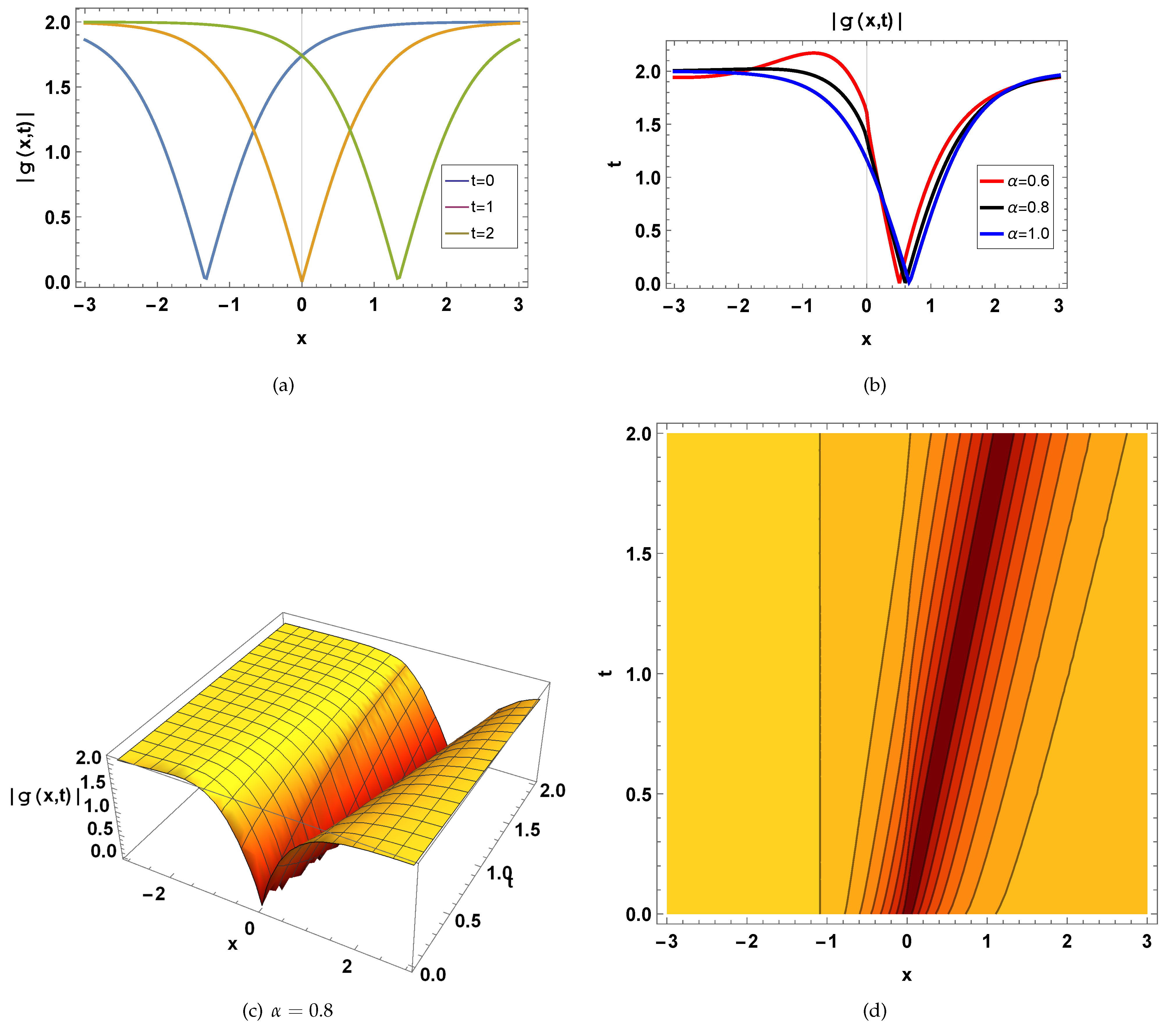
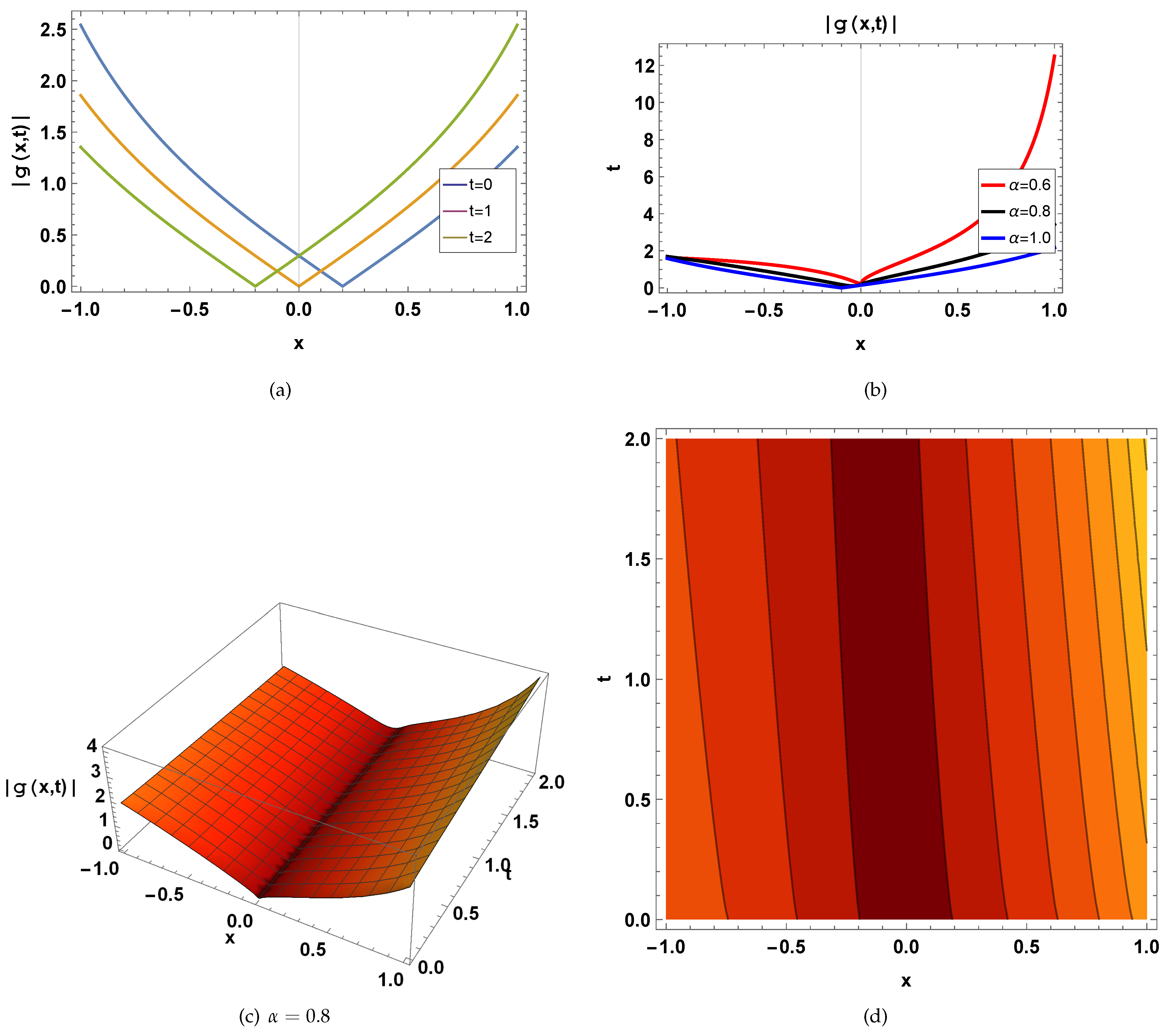
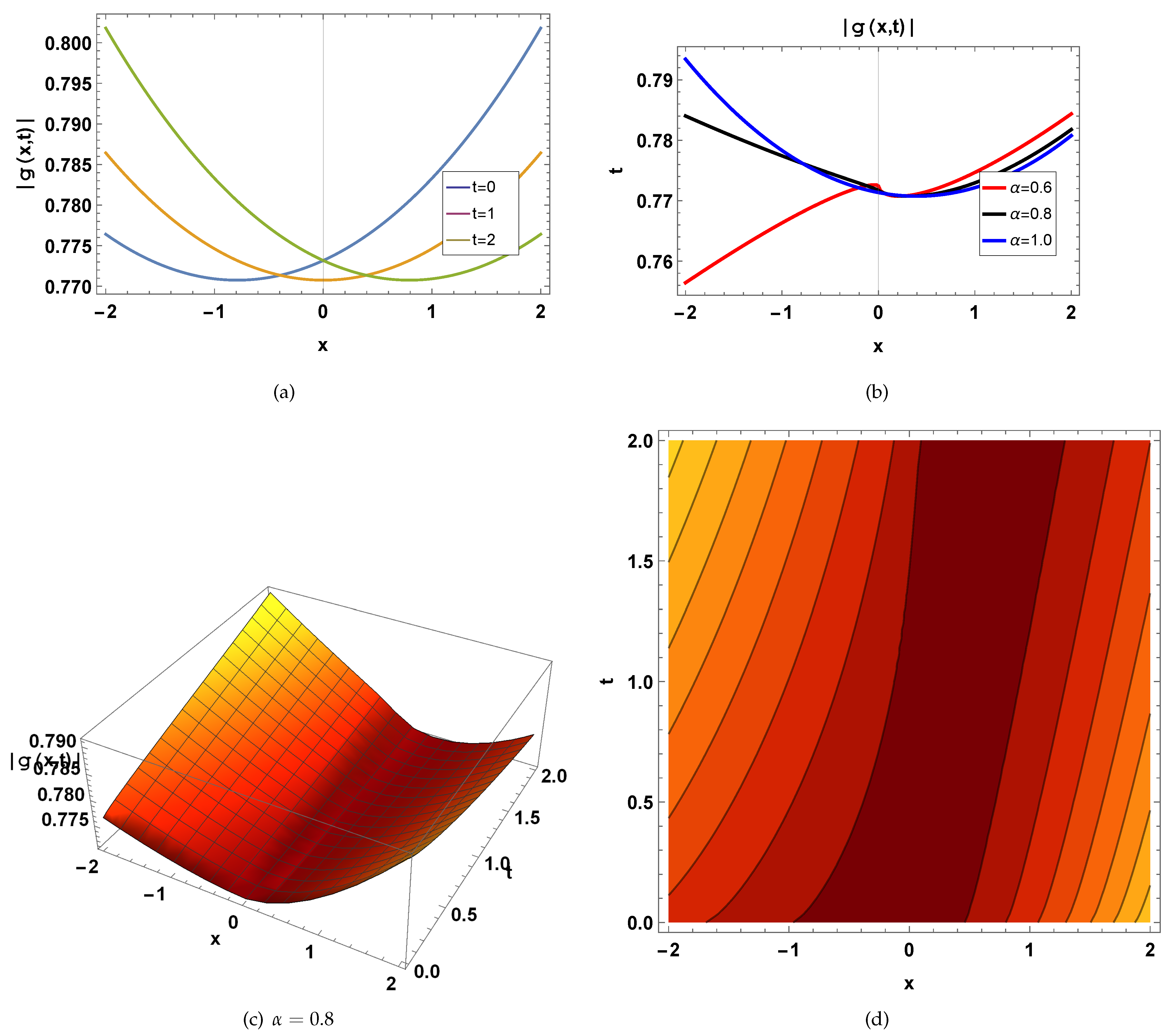
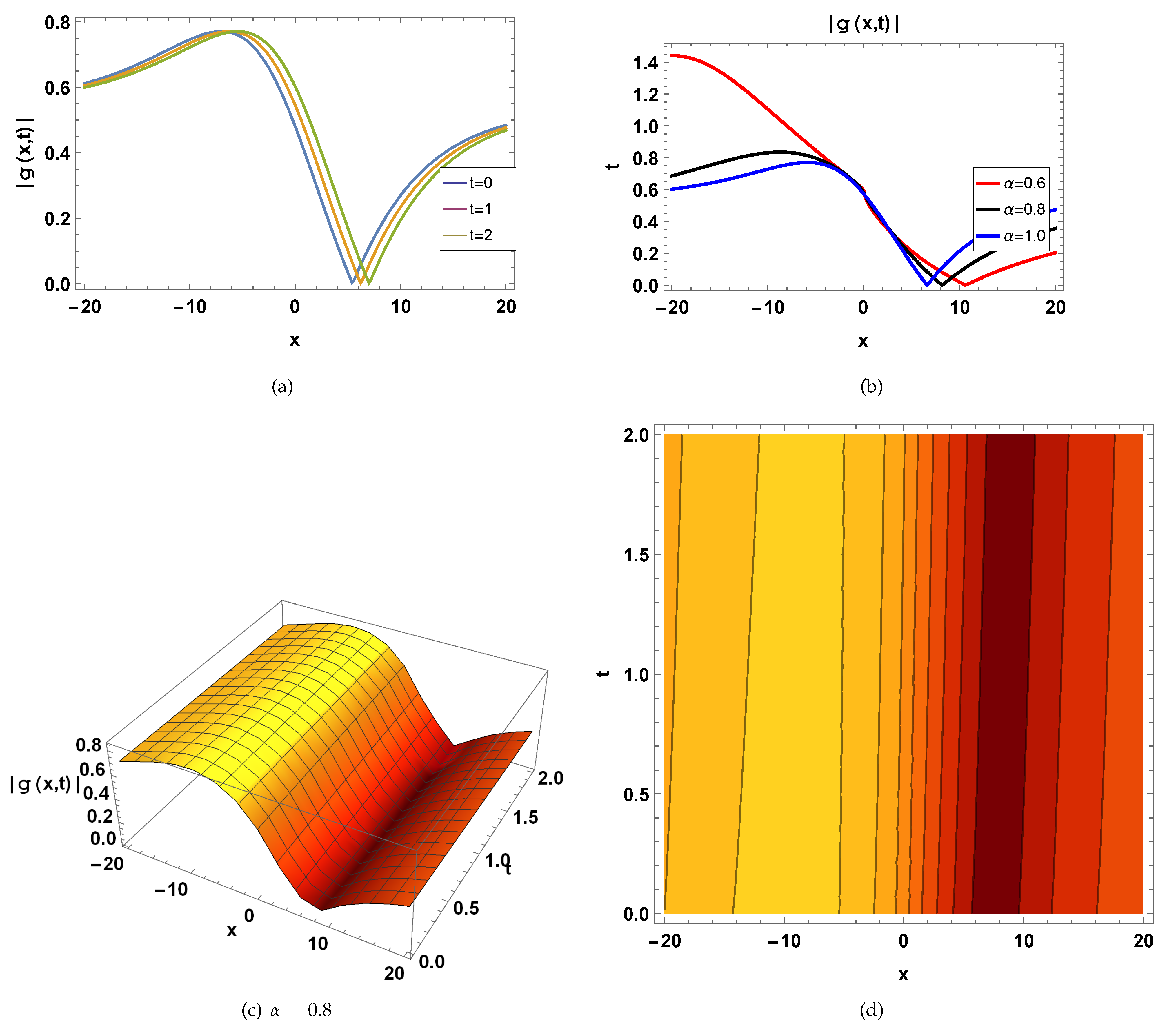
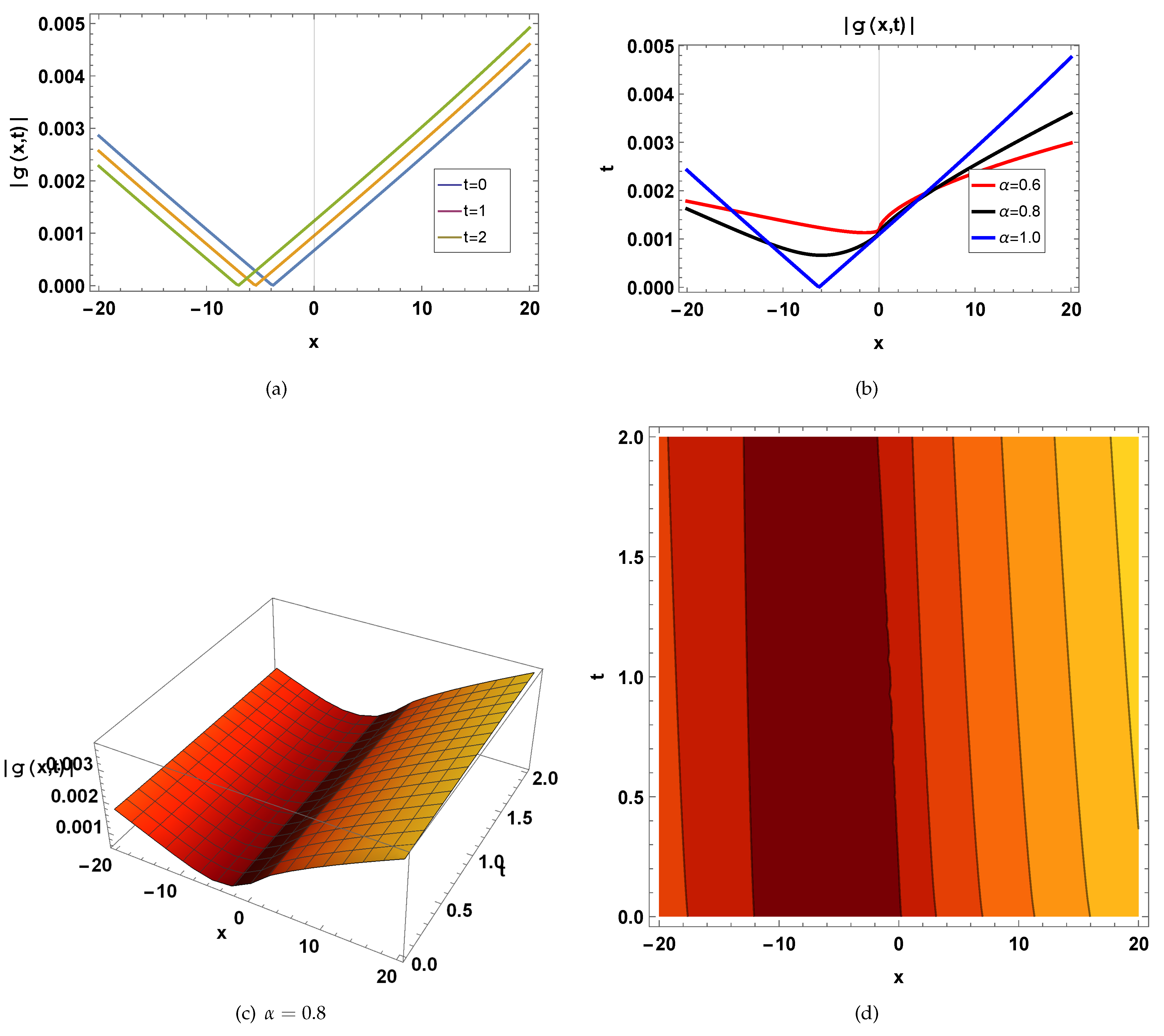
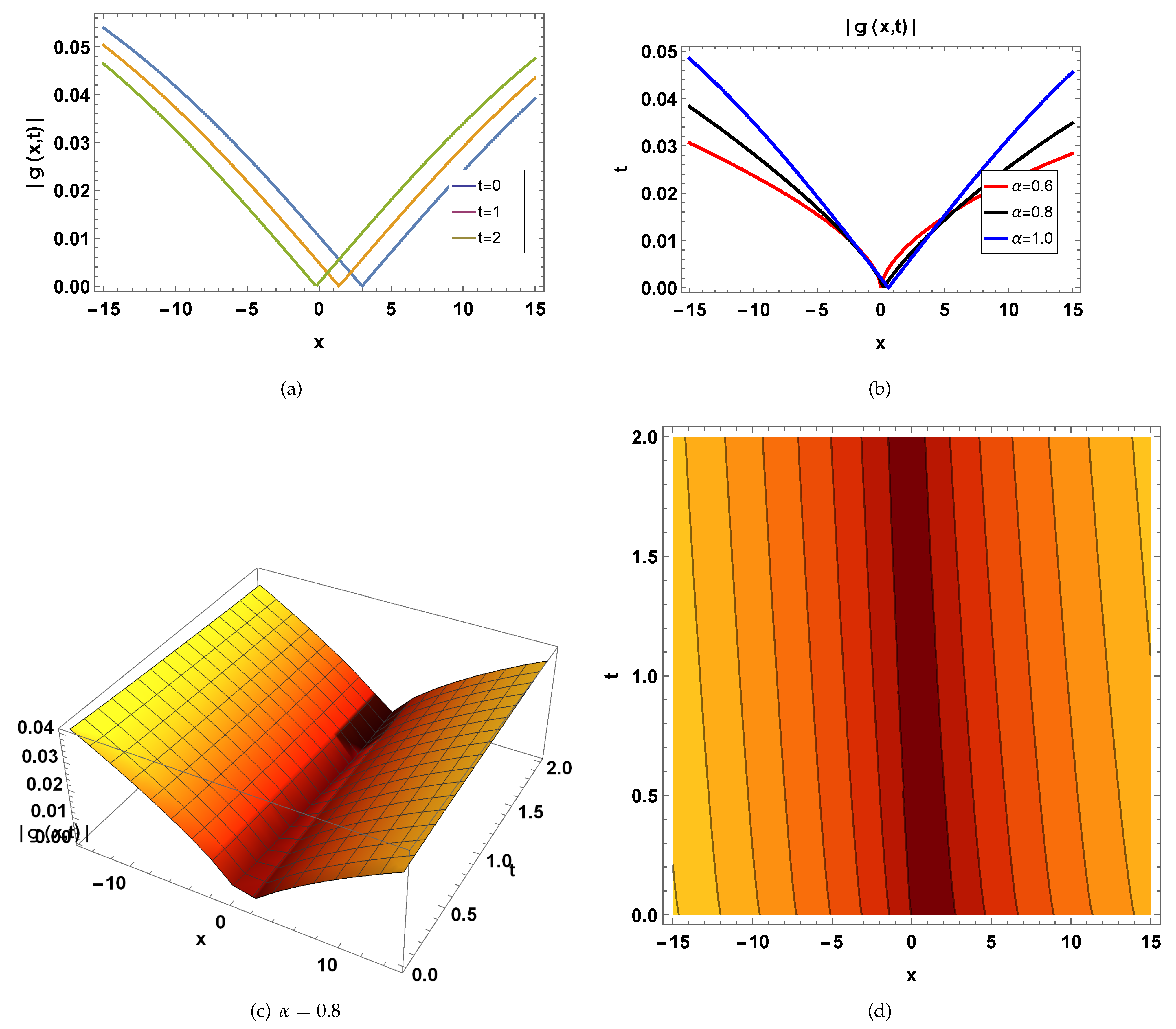
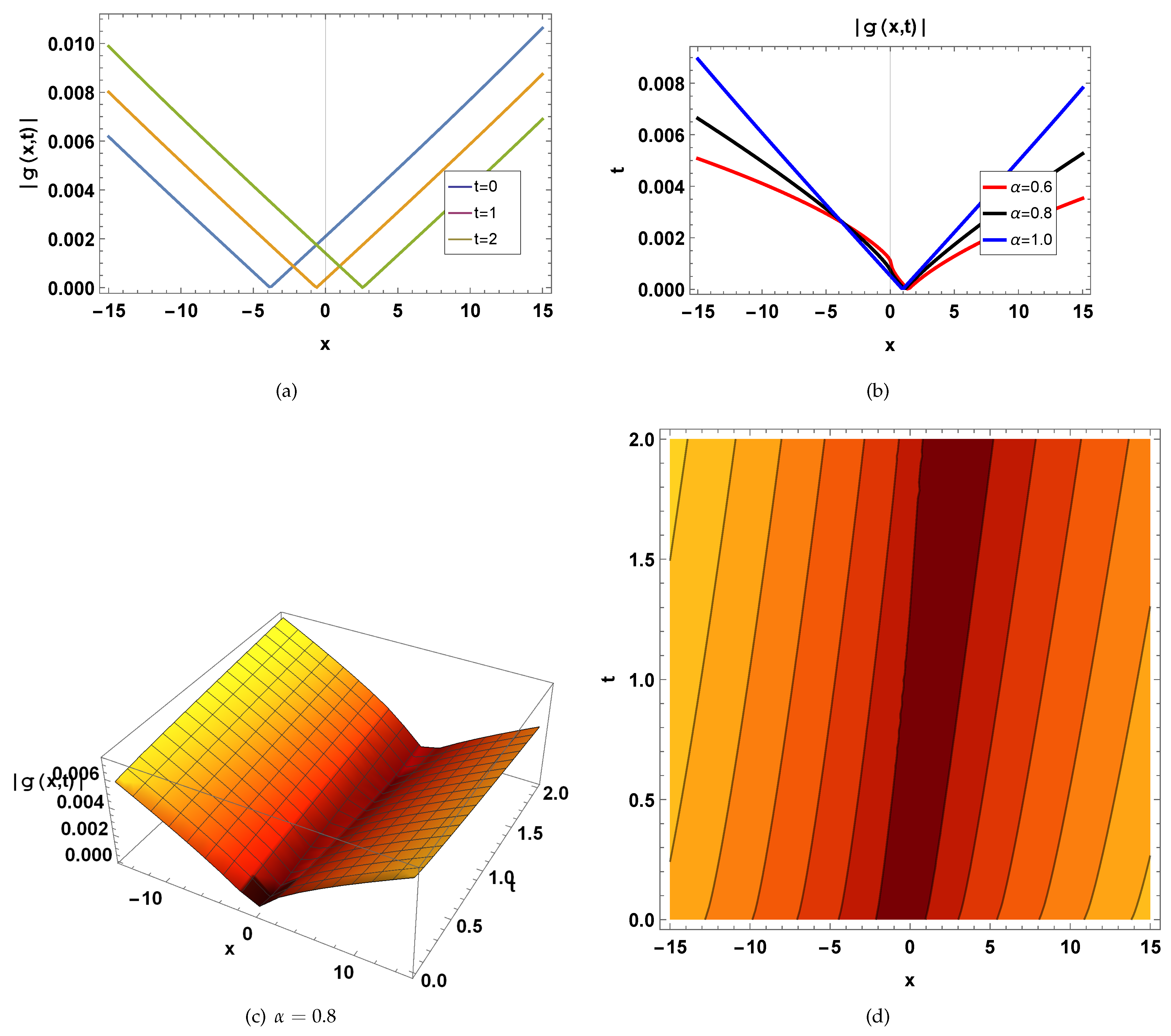
6. Physical Explanation

Here, we will explain few of the gained solutions by 2D, 3D, and contour graphs (Figure 1, Figure 2, Figure 3, Figure 4, Figure 5, Figure 6, Figure 7, Figure 8, Figure 9 and Figure 10).

Figure 1. The plot of $|g(x,t)|$ is given in Equation (25), which indicates the dark soliton at: $\mu =1,$ $\Omega =1,$ $\theta =-1,\mho =-1$, and ${\rm Y}=1$. (a) A 2D plot for $x\in (-3,3)$ for $\alpha =1$, where the blue line represents t = 0, the orange line represents t = 1, and the green line represents t = 2. (b) A 2D plot at $x\in (-3,3)$ and $t\in (0,2)$, with a red curve for $\alpha =0.6$, a black curve for $\alpha =0.8$, and a blue curve for $\alpha =1$. (c) A 3D graph for $\alpha =0.8$ at $t\in (0,2)$. (d) A contour plot for $\alpha =0.8$ at $t\in (0,2)$. The dark soliton solution has applications in optical communication, nonlinear optics, etc.

Figure 2. The plot of $|g(x,t)|$ is represented by Equation (30), which indicates the periodic wave solution at: $\mu =1,\Omega =0.01,\theta =0.1,\mho =0.6$, and ${\rm Y}=1$. (a) A 2D plot for $x\in (-1,1)$ for $\alpha =1$, where the blue line represents t = 0, the orange line represents t = 1, and the green line represents t = 2. (b) A 2D plot at $x\in (-1,1)$ and $t\in (0,2)$, with a red curve for $\alpha =0.6$, a black curve for $\alpha =0.8$, and a blue curve for $\alpha =1$. (c) A 3D graph for $\alpha =0.8$ at $t\in (0,2)$. (d) A contour plot for $\alpha =0.8$ at $t\in (0,2)$.

Figure 3. The plot of $|g(x,t)|$ is represented by Equation (37), which shows the dark soliton at: $\mu =1,\Omega =0.1,$ $\theta =0.02,$ $\omega =-0.5$, and ${\rm Y}=1$. (a) A 2D plot for $x\in (-2,2)$ for $\alpha =1$, where the blue line represents t = 0, the orange line represents t = 1, and the green line represents t = 2. (b) A 2D plot at $x\in (-2,2)$ and $t\in (0,2)$, with a red curve for $\alpha =0.6$, a black curve for $\alpha =0.8$, and a blue curve for $\alpha =1$. (c) A 3D graph when $\alpha =0.8$ at $t\in (0,2)$. (d) A contour plot for $\alpha =0.8$ at $t\in (0,2)$.

Figure 4. The wave function $|g(x,t)|$ is represented by Equation (69), which indicates the bright soliton at: $\mu =1,\Omega =1,\theta =0.2,\kappa =0.06$, and ${\rm Y}=1$. (a) A 2D plot for $x\in (-1,1)$ for $\alpha =1$, where the blue line represents t = 0, the orange line represents t = 1, and the green line represents t = 2. (b) A 2D plot at $x\in (-1,1)$ and $t\in (0,2)$, with a red curve for $\alpha =0.6$, a black curve for $\alpha =0.8$, and a blue curve for $\alpha =1$. (c) A 3D graph for $\alpha =0.8$ at $t\in (0,2)$. (d) A contour plot for $\alpha =0.8$ at $t\in (0,2)$. The bright soliton has applications in optical communication, wave transmission, nonlinear optics, etc.

Figure 5. The wave function of $|g(x,t)|$ is represented by Equation (71), which indicates the periodic wave solution with the following parameter values: $\mu =1,\Omega =1,\theta =0.04,\kappa =-0.01$, and ${\rm Y}=1$. (a) A 2D plot for $x\in (-2,2)$ for $\alpha =1$, where the blue line represents t = 0, the orange line represents t = 1, and the green line represents t = 2. (b) A 2D plot at $x\in (-2,2)$ and $t\in (0,2)$, with a red curve for $\alpha =0.6$, a black curve for $\alpha =0.8$, and a blue curve for $\alpha =1$. (c) A 3D graph for $\alpha =0.8$ at $t\in (0,2)$. (d) A contour plot for $\alpha =0.8$ at $t\in (0,2)$.

Figure 6. The wave function of $|g(x,t)|$ is represented by Equation (75), which indicates the dark-bright soliton solution with the following parameter values: $\mu =1,\Omega =0.2,\theta =0.04,\kappa =-0.01$, and ${\rm Y}=1$. (a) A 2D plot for $x\in (-20,20)$ for $\alpha =1$, where the blue line represents t = 0, the orange line represents t = 1, and the green line represents t = 2. (b) A 2D plot at $x\in (-20,20)$ and $t\in (0,2)$, with a red curve for $\alpha =0.6$, a black curve for $\alpha =0.8$, and a blue curve for $\alpha =1$. (c) A 3D graph for $\alpha =0.8$ at $t\in (0,2)$. (d) A contour plot for $\alpha =0.8$ at $t\in (0,2)$. The dark-bright soliton solution has many applications, including optical communication, nonlinear optics, condensed matter physics, and mathematical physics.

Figure 7. The wave function of $|g(x,t)|$ is represented by Equation (79), which indicates the double periodic wave solution with the following parameter values: $\mu =1,\Omega =0.1,\theta =0.4,\kappa =0.01$, and ${\rm Y}=1$. (a) A 2D plot for $x\in (-7,7)$ for $\alpha =1$, where the blue line represents t = 0, the orange line represents t = 1, and the green line represents t = 2. (b) A 2D plot at $x\in (-7,7)$ and $t\in (0,2)$, with a red curve for $\alpha =0.6$, a black curve for $\alpha =0.8$, and a blue curve for $\alpha =1$. (c) A 3D graph for $\alpha =0.8$ at $t\in (0,2)$. (d) A contour plot for $\alpha =0.8$ at $t\in (0,2)$.

Figure 8. The wave function of $|g(x,t)|$ is represented by Equation (108), which indicates the periodic wave solution with the following parameter values: $\mu =0.01,\Omega =-0.4;\theta =1,{\rm Y}=1,a=0.8,b=0.08,$ $c=0.5$, and $d_0=0.8$. (a) A 2D plot at $x\in (-20,20)$ for $\alpha =1$, where the blue line represents t = 0, the orange line represents t = 1, and the green line represents t = 2. (b) A 2D plot at $x\in (-20,20)$ and $t\in (0,2)$, with a red curve for $\alpha =0.6$, a black curve for $\alpha =0.8$, and a blue curve for $\alpha =1$. (c) A 3D graph for $\alpha =0.8$ at $t\in (0,2)$. (d) A contour plot for $\alpha =0.8$ at $t\in (0,2)$.

Figure 9. The wave function of $|g(x,t)|$ is represented by Equation (113), which indicates the singular soliton with the following parameter values: $\mu =1,\Omega =-0.4,\theta =1,{\rm Y}=1b=0.08,c=0.5$, and $d_0=0.8$. (a) A 2D graph for $x\in (-15,15)$ for $\alpha =1$, where the blue line represents t = 0, the orange line represents t = 1, and the green line represents t = 2. (b) A 2D plot at $x\in (-15,15)$ and $t\in (0,2)$, with a red curve for $\alpha =0.6$, a black curve for $\alpha =0.8$, and a blue curve for $\alpha =1$. (c) A 3D graph for $\alpha =0.8$ at $t\in (0,2)$. (d) A contour plot for $\alpha =0.8$ at $t\in (0,2)$. The singular soliton is used to describe the waves in oceans or shallow water, optical vortices, and magnetic materials.

Figure 10. The wave function of $|g(x,t)|$ represented by Equation (119), which indicates the periodic wave solution with the following parameter values: $\mu =0.10,\Omega =0.8,\theta =2,{\rm Y}=1,a=0.05,c=0.5$, and $d_0=2$. (a) A 2D graph at $x\in (-15,15)$ for $\alpha =1$, where the blue line represents t = 0, the orange line represents t = 1, and the green line represents t = 2. (b) A 2D plot at $x\in (-15,15)$ and $t\in (0,2)$, with a red curve for $\alpha =0.6$, a black curve for $\alpha =0.8$, and a blue curve for $\alpha =1$. (c) A 3D graph for $\alpha =0.8$ at $t\in (0,2)$. (d) A contour plot for $\alpha =0.8$ at $t\in (0,2)$. The periodic wave solution is used to describes the sound waves, light waves, water waves, etc.

7. Conclusions

We have successfully derived novel kinds of M-fractional wave solutions for the nonlinear simplified Modified Camassa–Holm model through the application of the modified simplest equation, the Sardar subequation, and the generalized Kudryashov techniques. These results open new forums for further research in this model, with potential applications in various areas in partial differential equations.

Our application of the modified simplest equation, the Sardar Subequation, and the generalized Kudryahov techniques has established their efficiency as straightforward, precise, and helpful tools for tackling nonlinear FPDEs. The simplicity of the provided solutions guarantees our understanding of the fundamental dynamics of this important mathematical physics model.

The obtained solutions have been thoroughly verified and further explained through the visualization of 2D, 3D, and contour plots, which were generated using the powerful Mathematica. These graphical representations not only confirm the cogency of our derived results but also offer valuable insight into the behavior of M-fractional wave solitons.

References

- Kuwayama, H.; Ishida, S. Biological soliton in multicellular movement. Sci. Rep. 2013, 3, 2272. [Google Scholar] [CrossRef] [PubMed]
- Cheng, C.D.; Tian, B.; Shen, Y.; Zhou, T. Bilinear form and Pfaffian solutions for a (2+ 1)-dimensional generalized Konopelchenko–Dubrovsky–Kaup–Kupershmidt system in fluid mechanics and plasma physics. Nonlinear Dyn. 2023, 111, 6659–6675. [Google Scholar] [CrossRef]
- Bilal, M.; Ahmad, J. New exact solitary wave solutions for the 3D-FWBBM model in arising shallow water waves by two analytical methods. Results Phys. 2021, 25, 104230. [Google Scholar]
- Alshahrani, B.; Yakout, H.A.; Khater, M.M.A.; Abdel-Aty, A.-H.; Mahmoud, E.E.; Baleanu, D.; Eleuch, H. Accurate novel explicit complex wave solutions of the (2+ 1)-dimensional Chiral nonlinear Schrödinger equation. Results Phys. 2021, 23, 104019. [Google Scholar] [CrossRef]
- Kudryashov, N.A. Method for finding highly dispersive optical solitons of nonlinear differential equations. Optik 2020, 206, 163550. [Google Scholar] [CrossRef]
- Hafez, M.G.; Alam, M.N.; Akbar, M.A. Exact traveling wave solutions to the Klein–Gordon equation using the novel (G′/G)-expansion method. Results Phys. 2014, 4, 177–184. [Google Scholar] [CrossRef]
- Tariq, K.U.; Ahmed, A.; Ma, W.-X. On some soliton structures to the Schamel–Korteweg-de Vries model via two analytical approaches. Mod. Phys. Lett. B 2022, 36, 2250137. [Google Scholar] [CrossRef]
- Tariq, K.U.; Zabihi, A.; Rezazadeh, H.; Younis, M.; Rizvi, S.T.R.; Ansari, R. On new closed form solutions: The (2+ 1)-dimensional Bogoyavlenskii system. Mod. Phys. Lett. B 2021, 35, 2150150. [Google Scholar] [CrossRef]
- Seadawy, A.R.; Alamri, S.Z. Mathematical methods via the nonlinear two-dimensional water waves of Olver dynamical equation and its exact solitary wave solutions. Results Phys. 2018, 8, 286–291. [Google Scholar] [CrossRef]
- Wang, Z.-Y.; Tian, S.-F.; Cheng, J. The ∂−-Dressing method and soliton solutions for the three-component coupled Hirota equations. J. Math. Phys. 2021, 62, 9. [Google Scholar] [CrossRef]
- Li, Y.; Tian, S.-F.; Yang, J.-J. Riemann–Hilbert problem and interactions of solitons in the-component nonlinear Schrödinger equations. Stud. Appl. Math. 2022, 148, 577–605. [Google Scholar] [CrossRef]
- Li, Z.-Q.; Tian, S.-F.; Yang, J.-J. On the soliton resolution and the asymptotic stability of N-soliton solution for the Wadati-Konno-Ichikawa equation with finite density initial data in space-time solitonic regions. Adv. Math. 2022, 409, 108639. [Google Scholar] [CrossRef]
- Razzaq, W.; Zafar, A.; Raheel, M. Searching the new exact wave solutions to the beta-fractional Paraxial nonlinear Schrödinger model via three different approaches. Int. J. Mod. Phys. B 2024, 38, 2450132. [Google Scholar] [CrossRef]
- Batool, F.; Rezazadeh, H.; Ali, Z.; Demirbilek, U. Exploring soliton solutions of stochastic Phi-4 equation through extended Sinh-Gordon expansion method. Opt. Quantum Electron. 2024, 56, 785. [Google Scholar] [CrossRef]
- Qawaqneh, H.; Manafian, J.; Alharthi, M.; Alrashedi, Y. Stability Analysis, Modulation Instability, and Beta-Time Fractional Exact Soliton Solutions to the Van der Waals Equation. Mathematics 2024, 12, 2257. [Google Scholar] [CrossRef]
- Gao, X.-T.; Tian, B.; Zhou, T.-Y.; Shen, Y.; Feng, C.-H. For the Shallow Water Waves: Bilinear-Form and Similarity-Reduction Studies on a Boussinesq-Burgers System. Int. J. Theor. Phys. 2024, 63, 1–10. [Google Scholar] [CrossRef]
- Dassios, G.; Vafeas, P. On the spheroidal semiseparation for stokes flow. Phys. Res. Int. 2008, 1, 135289. [Google Scholar] [CrossRef]
- Akbari, M. Exact solutions of the coupled Higgs equation and the Maccari system using the modified simplest equation method. Inf. Sci. Lett. 2013, 2, 155–158. [Google Scholar] [CrossRef]
- Kuo, C.-K. New solitary solutions of the Gardner equation and Whitham–Broer–Kaup equations by the modified simplest equation method. Optik 2017, 147, 128–135. [Google Scholar] [CrossRef]
- Murad, M.A.S.; Iqbal, M.; Arnous, A.H.; Yildirim, Y.; Jawad, A.J.A.M.; Hussein, L.; Biswas, A. Optical dromions for Radha–Lakshmanan model with fractional temporal evolution by modified simplest equation. J. Opt. 2024, 1–10. [Google Scholar] [CrossRef]
- Debin, K.; Rezazadeh, H.; Ullah, N.; Vahidi, J.; Tariq, K.U.; Akinyemi, L. New soliton wave solutions of a (2+ 1)-dimensional Sawada-Kotera equation. J. Ocean. Eng. Sci. 2022, 8, 527–532. [Google Scholar] [CrossRef]
- Cinar, M.; Secer, A.; Ozisik, M.; Bayram, M. Derivation of optical solitons of dimensionless Fokas-Lenells equation with perturbation term using Sardar sub-equation method. Opt. Quantum Electron. 2022, 54, 402. [Google Scholar] [CrossRef]
- Tariq, M.M.; Riaz, M.B.; Aziz-ur-Rehman, M. Investigation of space-time dynamics of Akbota equation using Sardar sub-equation and Khater methods: Unveiling bifurcation and chaotic structure. Int. J. Theor. Phys. 2024, 63, 210. [Google Scholar] [CrossRef]
- Barman, H.K.; Roy, R.; Mahmud, F.; Akbar, M.A.; Osman, M.S. Harmonizing wave solutions to the Fokas-Lenells model through the generalized Kudryashov method. Optik 2021, 229, 166294. [Google Scholar] [CrossRef]
- Pandir, Y.; Sahragül, E. Exact solutions of the two dimensional KdV-Burger equation by generalized Kudryashov method. J. Inst. Sci. Technol. 2021, 11, 617–624. [Google Scholar] [CrossRef]
- Aydın, Z.; Taşcan, F. Application of the generalized Kudryashov method to the Kolmogorov-Petrovskii-Piskunov equation. Eskişehir Tech. Univ. J. Sci. Technol. A Appl. Sci. Eng. 2024, 25, 320–330. [Google Scholar] [CrossRef]
- Alam, M.N.; Akbar, M.A. Some new exact travelling wave solutions to the simplified MCH equation and the (1+1)-dimensional combined KdV-mKdV equations. J Assoc. Arab. Univ. Basic Appl. Sci. 2015, 17, 6–13. [Google Scholar]
- Zulfiqar, A.; Ahmad, J. Exact solitary wave solutions of fractional modified Camassa–Holm equation using an efficient method. Alexandra Eng. J. 2020, 59, 3565–3574. [Google Scholar] [CrossRef]
- Hassan, S.Z.; Abdelrahman, M.A. Solitary wave solutions for some nonlinear time-fractional partial differential equations. Pramana 2018, 91, 67. [Google Scholar] [CrossRef]
- Devnath, S.; Khan, S.; Akbar, M.A. Exploring solitary wave solutions to the simplified modified camassa-holm equation through a couple sophisticated analytical approaches. Results Phys. 2024, 59, 107580. [Google Scholar] [CrossRef]
- Khatun, M.M.; Akbar, M.A. Analytical soliton solutions of the beta time-fractional simplified modified Camassa-Holm equation in shallow water wave propagation. J. Umm -Qura Univ. Appl. Sci. 2024, 10, 120–128. [Google Scholar] [CrossRef]
- Wazwaz, A.M. Solitary wave solutions for modified forms of Degasperis–Procesi and Camassa–Holm equations. Phys. Lett. A 2006, 352, 500–504. [Google Scholar] [CrossRef]
- Zafar, A.; Raheel, M.; Hosseini, K.; Mirzazadeh, M.; Salahshour, S.; Park, C.; Shin, D.Y. Diverse approaches to search for solitary wave solutions of the fractional modified Camassa–Holm equation. Results Phys. 2021, 31, 104882. [Google Scholar] [CrossRef]
- Sulaiman, T.A.; Yel, G.; Bulut, H. M-fractional solitons and periodic wave solutions to the Hirota- Maccari system. Mod. Phys. Lett. B 2019, 33, 1950052. [Google Scholar] [CrossRef]
- Sousa, J.V.D.C.; de Oliveira, E.C. A new truncated M-fractional derivative type unifying some fractional derivative types with classical properties. Int. J. Anal. Appl. 2018, 16, 83–96. [Google Scholar]
- Ullah, N.; Asjad, M.I.; Awrejcewicz, J.; Muhammad, T.; Baleanu, D. On soliton solutions of fractional-order nonlinear model appears in physical sciences. AIMS Math. 2022, 7, 7421–7440. [Google Scholar] [CrossRef]
- Kudryashov, N.A. One method for finding exact solutions of nonlinear differential equations. Commun. Nonlinear Sci. Numer. Simul. 2012, 17, 2248–2253. [Google Scholar] [CrossRef]
- Gaber, A.A.; Aljohani, A.F.; Ebaid, A.; Machado, J.T. The generalized Kudryashov method for nonlinear space-time fractional partial differential equations of burgers type. Nonlinear Dyn. 2019, 95, 361–368. [Google Scholar] [CrossRef]
- Gómez, C.A.; Salas, A.H. Special symmetries to standard Riccati equations and applications. Appl. Math. Comput. 2010, 216, 3089–3096. [Google Scholar] [CrossRef]
Disclaimer/Publisher’s Note: The statements, opinions and data contained in all publications are solely those of the individual author(s) and contributor(s) and not of MDPI and/or the editor(s). MDPI and/or the editor(s) disclaim responsibility for any injury to people or property resulting from any ideas, methods, instructions or products referred to in the content. |
© 2024 by the authors. Licensee MDPI, Basel, Switzerland. This article is an open access article distributed under the terms and conditions of the Creative Commons Attribution (CC BY) license (https://creativecommons.org/licenses/by/4.0/).