


Excessive External Borrowing in China: Evidence from a Nonparametric Threshold Regression Model with Fixed Effects


Abstract
1. Introduction
2. Empirical Model
2.1. Nonparametric Panel Threshold Regression
2.2. Parametric Panel Threshold Regression
2.3. Hypothesis Testing
3. Data
4. Empirical Results
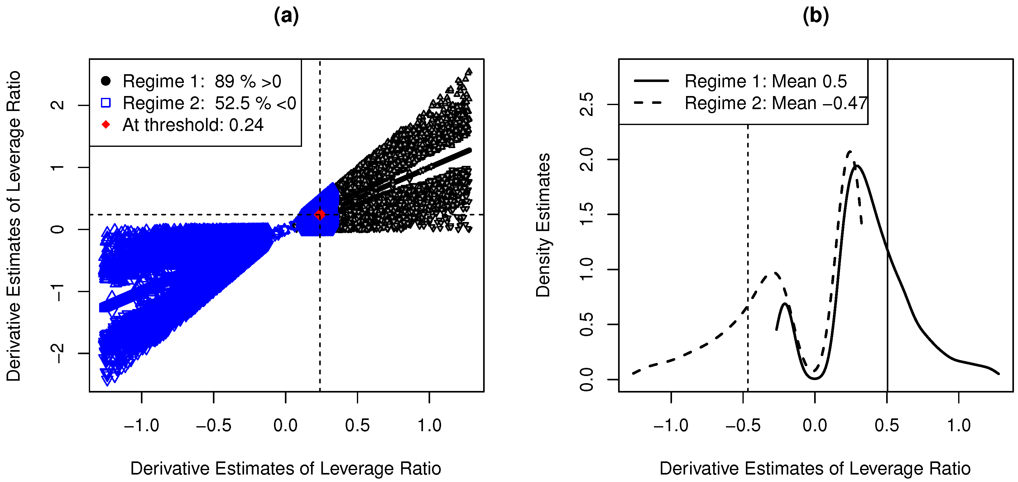
4.1. Whole Sample
4.2. By Ownerships
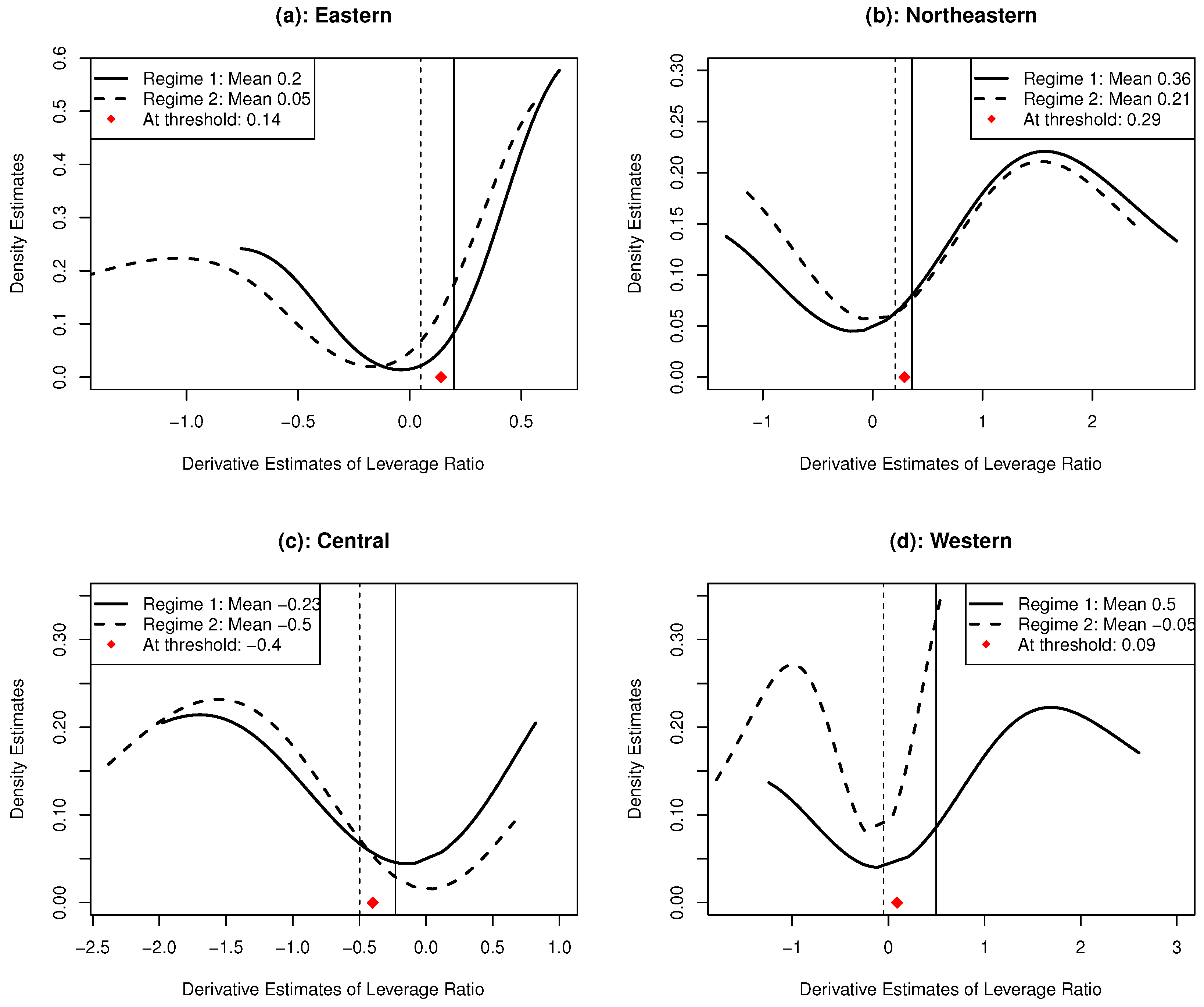
4.3. By Region
5. Robustness Check: An Alternative Indicator of External Financing
6. Conclusions
Author Contributions
Funding
Data Availability Statement
Acknowledgments
Conflicts of Interest
Appendix A. Simulation Results of NPTM-FE
- (1)
- (2)
- Generate wild-bootstrap residuals , where for each observation and , with probability and with probability , where . Construct the bootstrap sample , where .
- (3)
- Compute similarly as in (1), but replace with .
- (4)
- Repeat steps (2) and (3) a large number (B) of times to obtain the empirical standard deviation of .

| Panel A | |||||||||||||
| () | |||||||||||||
| DGP 1 | (n,T) | RMSE | BIAS | RMSE | BIAS | RMSE | BIAS | RMSE | BIAS | RMSE | BIAS | RMSE | BIAS |
| (50,10) | 0.1295 | 0.0973 | 0.1394 | 0.1094 | 0.0302 | 0.0245 | 0.0761 | 0.0523 | 0.0889 | 0.0599 | 0.0907 | 0.0610 | |
| (100,10) | 0.0959 | 0.0707 | 0.0985 | 0.0757 | 0.0287 | 0.0141 | 0.0540 | 0.0311 | 0.0638 | 0.0410 | 0.0788 | 0.0453 | |
| (200,10) | 0.0636 | 0.0514 | 0.0781 | 0.0532 | 0.0089 | 0.0015 | 0.0301 | 0.0155 | 0.0468 | 0.0272 | 0.0522 | 0.0336 | |
| DGP 2 | |||||||||||||
| (50,10) | 0.1333 | −0.1131 | 0.1428 | −0.1106 | 0.0627 | 0.0436 | 0.0635 | 0.0444 | 0.0988 | 0.0711 | 0.0994 | 0.0814 | |
| (100,10) | 0.1051 | −0.0792 | 0.1184 | −0.0846 | 0.0426 | 0.0212 | 0.0469 | 0.0233 | 0.0721 | 0.0550 | 0.0805 | 0.0629 | |
| (200,10) | 0.0770 | −0.0408 | 0.0866 | −0.0515 | 0.0205 | 0.0099 | 0.0260 | 0.0146 | 0.0512 | 0.0325 | 0.0598 | 0.0340 | |
| Panel B | |||||||||||||
| () | C = 1.5 | C = 1.5 | C = 1.5 | ||||||||||
| DGP 1 | (n,T) | RMSE | BIAS | RMSE | BIAS | RMSE | BIAS | RMSE | BIAS | RMSE | BIAS | RMSE | BIAS |
| (50,10) | 0.1433 | 0.0946 | 0.1428 | 0.1031 | 0.0351 | 0.0237 | 0.0782 | 0.0241 | 0.0941 | 0.0584 | 0.1081 | 0.0652 | |
| (100,10) | 0.1029 | 0.0704 | 0.1151 | 0.0756 | 0.0290 | 0.0139 | 0.0594 | 0.0159 | 0.0722 | 0.0402 | 0.0798 | 0.0455 | |
| (200,10) | 0.0766 | 0.0505 | 0.0770 | 0.0541 | 0.0093 | 0.0012 | 0.0334 | 0.0019 | 0.0499 | 0.0253 | 0.0512 | 0.0285 | |
| DGP 2 | |||||||||||||
| (50,10) | 0.1412 | −0.0488 | 0.1556 | −0.1176 | 0.0720 | 0.0432 | 0.0635 | 0.0444 | 0.0994 | 0.0703 | 0.1123 | 0.0838 | |
| (100,10) | 0.1064 | −0.0105 | 0.1213 | −0.0803 | 0.0513 | 0.0208 | 0.0469 | 0.0233 | 0.0715 | 0.0505 | 0.0845 | 0.0521 | |
| (200,10) | 0.0751 | −0.0076 | 0.0853 | −0.0604 | 0.0241 | 0.0091 | 0.0260 | 0.0146 | 0.0485 | 0.0297 | 0.0526 | 0.0314 | |
Appendix B. Bootstrap Procedure for Testing the Correct Specification of PTM-FE
- 1.
- Given the estimated threshold value in (6) under PTM-FE in (10), use the original sample to compute in (12), with defined in (10). Obtain the residual as defined in Section 2.3.
- 2.
- Generate the wild-bootstrap residual , where for each observation and , with probability and with probability . Then, construct the bootstrapped independent variable , with the estimated parameters obtained from PTM-FE in (10). Call the bootstrapped sample.
- 3.
- Compute as in step 1, except with the original sample replaced by the bootstrapped sample .
- 4.
- Repeat steps 2–3 a large number times (B) to obtain . Reject if , where is the upper percentile value of its empirical distribution, and is the significance level.
Appendix C. Chinese Industrial Two-Digit Classification Codes
| CICC | Industry Name |
| 6 | Exploration and abstention of coal and char industry |
| 7 | Exploration of oil and natural gas industry |
| 8 | Picking of ferrous metal mine industry |
| 9 | Picking of non-ferrous metal mine industry |
| 10 | Picking of non-metal mine industry |
| 11 | Other mining industry |
| 13 | Agriculture and food processing industry |
| 14 | Foodstuff manufacturing industry |
| 15 | Soft drink manufacturing industry |
| 16 | Tobacco manufacturing industry |
| 17 | Textile industry |
| 18 | Waving costume, shoes and cap manufacturing industry |
| 19 | Leather, fur and feather manufacturing industry |
| 20 | Wood working, and wood, bamboo, bush rope, palm, and straw manufacturing industry |
| 21 | Furniture manufacturing industry |
| 22 | Paper making and paper products industry |
| 23 | Print and copy of record vehicle industry |
| 24 | Stationary and sporting goods manufacturing industry |
| 25 | Oil processing, coking and nuclear manufacturing industry |
| 26 | Chemical material and chemical product manufacturing industry |
| 27 | Medicine manufacturing industry |
| 28 | Chemical fiber manufacturing industry |
| 29 | Rubber product industry |
| 30 | Plastics product industry |
| 31 | Non-metallic mineral product industry |
| 32 | Ferrous metal refining and calendaring processing industry |
| 33 | Non-ferrous metal refining and calendaring processing industry |
| 34 | Metal product industry |
| 35 | Universal equipment manufacturing industry |
| 36 | Task equipment manufacturing industry |
| 37 | Transport and communication facilities manufacturing industry |
| 39 | Electric machine and fittings manufacturing industry |
| 40 | Communication apparatus, computer and other electric |
| installation manufacturing industry | |
| 41 | Instrument and meter, stationery machine manufacturing industry |
| 42 | Handicraft and other manufacturing industry |
| 43 | Removal and processing of obsolete resource and material industry |
| 44 | Electricity and thermal manufacturing and supplying industry |
| 45 | Combustion gas manufacturing and supplying industry |
| 46 | Water manufacturing and supplying industry |
| Note: CICC refers to two-digit industry classification code based on NBSC. Industries are mainly classified as manufacturing (CICC 13–43), mining (CICC 6–11), and public utility industries (CICC 44–46). | |
Appendix D. Geographic-Based Region Classification
| Eastern Region | Beijing | Tianjin | Hebei | Shanghai | Jiangsu |
| Zhejiang | Shandong | Fujian | Guangdong | Hainan | |
| Northeastern Region | Liaoning | Jilin | Heilongjiang | ||
| Central Region | Shanxi | Anhui | Jiangxi | Henan | Hubei |
| Hunan | |||||
| Western Region | Neimenggu | Guangxi | Chongqing | Sichuan | Guizhou |
| Yunnan | Tibet | Shǎnxi | Gansu | Qinghai | |
| Ningxia | Xinjiang | ||||
| Note: Region classification is on the basis of the National Bureau of Statistics of China. | |||||
Appendix E. Percentage of Firm Ownership Types Across Regions
| Eastern Region | Western Region | Central Region | Northeastern Region | |
| SOEs | 9.6% | 31.8% | 30.3% | 20.4% |
| Private firms | 41.5% | 27.6% | 42.5% | 27.8% |
| Collective firms | 14% | 11.7% | 18.6% | 10.3% |
| Foreign firms | 34.9% | 28.9% | 8.6% | 41.5% |
Appendix F. Descriptive Data Summary for Leverage Growth (LG)
| Percentile | 10% | 25% | 50% | 75% | 90% | Mean |
| whole sample | −0.3176 | −0.112 | 0.0416 | 0.2825 | 0.7378 | 0.5041 |
| By ownership | ||||||
| SOEs | −0.235 | −0.071 | 0.0392 | 0.2109 | 0.5591 | 0.372 |
| private | −0.2738 | −0.0905 | 0.0543 | 0.2996 | 0.7349 | 0.3603 |
| foreign | −0.3967 | −0.1645 | 0.0344 | 0.3165 | 0.8393 | 0.7239 |
| collective | −0.293 | −0.0978 | 0.0263 | 0.229 | 0.6411 | 0.3393 |
| By region | ||||||
| eastern | −0.3173 | −0.1165 | 0.0438 | 0.2866 | 0.7225 | 0.4377 |
| western | −0.3256 | −0.1033 | 0.0434 | 0.2869 | 0.781 | 0.9073 |
| northeastern | −0.3501 | −0.1316 | 0.0334 | 0.2839 | 0.8471 | 0.3173 |
| central | −0.2887 | −0.0813 | 0.031 | 0.248 | 0.7835 | 0.6228 |
Appendix G. Limitations
References
- King, R.G.; Levine, R. Finance, entrepreneurship and growth. J. Monet. Econ. 1993, 32, 513–542. [Google Scholar] [CrossRef]
- Demirguc-Kunt, A.; Maksimovic, V. Law, finance, and firm growth. J. Financ. 1998, 53, 2107–2137. [Google Scholar] [CrossRef]
- Rajan, R.; Zingales, L. Financial dependence and growth. Am. Econ. Rev. 1998, 88, 559–586. [Google Scholar]
- Chen, M.; Guariglia, A. Internal financial constraints and firm productivity in China: Do liquidity and export behavior make a difference? J. Comp. Econ. 2013, 41, 1123–1140. [Google Scholar] [CrossRef]
- Guariglia, A.; Liu, X.; Song, L. Internal finance and growth: Microeconometric evidence on Chinese firms. J. Dev. Econ. 2011, 96, 79–94. [Google Scholar] [CrossRef]
- Bai, Y.; Lu, D.; Tian, X. Do Financial Frictions Explain Chinese Firm Saving and Misallocation? Working Paper; National Bureau of Economic Research: Cambridge, MA, USA, 2016. [Google Scholar]
- Ding, S.; Guariglia, A.; Harris, R. The determinants of productivity in Chinese large and medium-sized industrial firms, 1998–2007. J. Product. Anal. 2016, 45, 131–155. [Google Scholar] [CrossRef]
- Song, Z.; Storesletten, K.; Zilibotti, F. Growing like China. Am. Econ. Rev. 2011, 101, 196–233. [Google Scholar] [CrossRef]
- Lin, J.Y.; Cai, F.; Li, Z. The China Miracle: Development Strategy and Economic Reform; Chinese University Press: Hong Kong, China, 2003. [Google Scholar]
- Ma, G.; Laurenceson, J. China’s Debt Challenge: Stylized facts, drivers and policy implications. Singap. Econ. Rev. 2019, 64, 815–837. [Google Scholar] [CrossRef]
- Lipton, D. Rebalancing China: International lessons in corporate debt. In Proceedings of the Conference on Sustainable Development in China and the World, China Economic Society, Shenzhen, China, 10–12 June 2016; Volume 10. [Google Scholar]
- Maliszewski, W.; Arslanalp, S.; Caparusso, J.; Garrido, J.; Guo, S.; Kang, J.S.; Lam, R.; Law, D.; Liao, W.; Rendak, N.; et al. Resolving China’s Corporate Debt Problem; International Monetary Fund: Washington, DC, USA, 2016. [Google Scholar]
- Modigliani, F.; Miller, M.H. The cost of capital, corporation finance and the theory of investment. Am. Econ. Rev. 1958, 48, 261–297. [Google Scholar]
- Allen, F.; Qian, J.; Qian, M. Law, finance, and economic growth in China. J. Financ. Econ. 2005, 77, 57–116. [Google Scholar] [CrossRef]
- Jin, M.; Zhao, S.; Kumbhakar, S.C. Financial constraints and firm productivity: Evidence from Chinese manufacturing. Eur. J. Oper. Res. 2019, 275, 1139–1156. [Google Scholar] [CrossRef]
- Giannetti, C. Relationship lending and firm innovativeness. J. Empir. Financ. 2012, 19, 762–781. [Google Scholar] [CrossRef]
- Garriga, J.M. The Effect of Relationship Lending on Firm Performance; Working Paper; Universitat Autònoma de Barcelona: Barcelona, Spain, 2006. [Google Scholar]
- Lang, L.; Ofek, E.; Stulz, R. Leverage, investment, and firm growth. J. Financ. Econ. 1996, 40, 3–29. [Google Scholar] [CrossRef]
- Huang, G. The determinants of capital structure: Evidence from China. China Econ. Rev. 2006, 17, 14–36. [Google Scholar] [CrossRef]
- Agostino, M.; Ruberto, S.; Trivieri, F. Lasting lending relationships and technical efficiency: Evidence on European SMEs. J. Product. Anal. 2004, 50, 25–40. [Google Scholar] [CrossRef]
- Gomis, R.M.; Khatiwada, S. Debt and Productivity: Evidence from Firm-Level Data; Working Paper; Graduate Institute of International and Development Studies: Geneva, Switzerland, 2017. [Google Scholar]
- Xiao, G. Nonperforming debts in Chinese enterprises: Patterns, causes, and implications for banking reform. Asian Econ. Pap. 2005, 4, 61–113. [Google Scholar] [CrossRef]
- Coricelli, F.; Driffield, N.; Pal, S.; Roland, I. When does leverage hurt productivity growth? a firm-level analysis. J. Int. Money Financ. 2012, 31, 1674–1694. [Google Scholar] [CrossRef]
- Levinsohn, J.; Petrin, A. Estimating production functions using inputs to control for unobservables. Rev. Econ. Stud. 2003, 70, 317–341. [Google Scholar] [CrossRef]
- Hansen, B.E. Threshold effects in non-dynamic panels: Estimation, testing, and inference. J. Econom. 1999, 93, 345–368. [Google Scholar] [CrossRef]
- Hansen, B.E. Sample Splitting and Threshold Estimation. Econometrica 2000, 68, 575–603. [Google Scholar] [CrossRef]
- Ma, Y.; Tang, H.; Zhang, Y. Factor intensity, product switching, and productivity: Evidence from Chinese exporters. J. Int. Econ. 2014, 92, 349–362. [Google Scholar] [CrossRef]
- Yu, P. Consistency of the least squares estimator in threshold regression with endogeneity. Econ. Lett. 2015, 131, 41–46. [Google Scholar] [CrossRef]
- Caner, M.; Hansen, B.E. Instrumental variable estimation of a threshold model. Econom. Theory 2004, 20, 813–843. [Google Scholar] [CrossRef]
- Yu, P. Inconsistency of 2SLS estimators in threshold regression with endogeneity. Econ. Lett. 2013, 120, 532–536. [Google Scholar] [CrossRef]
- Yu, P.; Phillips, P.C.B. Threshold regression with endogeneity. J. Econom. 2018, 203, 50–68. [Google Scholar] [CrossRef]
- Sun, Y.; Carroll, R.J.; Li, D. Semiparametric estimation of fixed-effects panel data varying coefficient models. In Nonparametric Econometric Methods; Emerald Group Publishing Limited: Bingley, UK, 2009; pp. 101–129. [Google Scholar]
- Su, L.; Ullah, A. Local polynomial estimation of nonparametric simultaneous equations models. J. Econom. 2008, 144, 193–218. [Google Scholar] [CrossRef]
- Drehmann, M.; Juselius, M. Evaluating early warning indicators of banking crises: Satisfying policy requirements. Int. J. Forecast. 2014, 30, 759–780. [Google Scholar] [CrossRef]
- Walter, C.; Howie, F. Red Capitalism: The Fragile Financial Foundation of China’s Extraordinary Rise; John Wiley: Singapore, 2012. [Google Scholar]
- Pettis, M. Avoiding the Fall: China’s Economic Restructuring; Brookings Institution Press: Washington, DC, USA, 2013. [Google Scholar]
- Liu, H. Three critical battles China is preparing to fight. In Proceedings of the World Economic Forum Annual Meeting, Davos, Switzerland, 23–26 January 2018. [Google Scholar]
- Bekaert, G.; Wu, G. Asymmetric volatility and risk in equity markets. Rev. Financ. Stud. 2000, 13, 1–42. [Google Scholar] [CrossRef]
- Alfaro, L.; Chanda, A.; Kalemli-Ozcan, S.; Sayek, S. FDI and economic growth: The role of local financial markets. J. Int. Econ. 2004, 64, 89–112. [Google Scholar] [CrossRef]
- Munir, Q.; Kok, S.C.; Teplova, T.; Li, T. Powerful CEOs, debt financing, and leasing in Chinese SMEs: Evidence from threshold model. N. Am. J. Econ. Financ. 2017, 42, 487–503. [Google Scholar] [CrossRef]
- Severance-Lossin, E.; Sperlich, S.A. Estimation of derivatives for additive separable models. Statistics 1999, 33, 241–265. [Google Scholar] [CrossRef]
- Lin, Z.; Li, Q.; Sun, Y. A consistent nonparametric test of parametric regression functional form in fixed effects panel data models. J. Econom. 2014, 178, 167–179. [Google Scholar] [CrossRef]
- Brandt, L.; Van Biesebroeck, J.; Wang, L.; Zhang, Y. Challenges of working with the Chinese NBS firm-level data. China Econ. Rev. 2014, 30, 339–352. [Google Scholar] [CrossRef]
- Ding, S.; Knight, J.; Zhang, X. Does China overinvest? Evidence from a panel of Chinese firms. Eur. J. Financ. 2016, 25, 489–507. [Google Scholar] [CrossRef]
- Cai, H.; Liu, Q. Competition and corporate tax avoidance: Evidence from Chinese industrial firms. Econ. J. 2009, 119, 764–795. [Google Scholar] [CrossRef]
- Berkowitz, D.; Ma, H.; Nishioka, S. Recasting the iron rice bowl: The reform of China’s state-owned enterprises. Rev. Econ. Stat. 2017, 99, 735–747. [Google Scholar] [CrossRef]
- Brandt, L.; Van Biesebroeck, J.; Wang, L.; Zhang, Y. WTO accession and performance of chinese manufacturing firms. Am. Econ. Rev. 2017, 107, 2784–2820. [Google Scholar] [CrossRef]
- Hsieh, C.T.; Klenow, P.J. Misallocation and manufacturing TFP in China and India. Q. J. Econ. 2009, 124, 1403–1448. [Google Scholar] [CrossRef]
- Wu, Y.; Zhou, X. Technical efficiency in the Chinese textile industry. Front. Econ. China 2013, 8, 146–163. [Google Scholar]
- Zhang, R.; Sun, K.; Delgado, M.S.; Kumbhakar, S.C. Productivity in China’s high technology industry: Regional heterogeneity and R&D. Technol. Forecast. Soc. Chang. 2012, 79, 127–141. [Google Scholar]
- Li, K.; Yue, H.; Zhao, L. Ownership, institutions, and capital structure: Evidence from China. J. Comp. Econ. 2009, 37, 471–490. [Google Scholar] [CrossRef]
- Kornai, J.; Maskin, E.; Roland, G. Understanding the soft budget constraint. J. Econ. Lit. 2003, 41, 1095–1136. [Google Scholar] [CrossRef]
- Riedel, J.; Jin, J.; Gao, J. How China Grows: Investment, Finance, and Reform; Princeton University Press: Princeton, NJ, USA, 2007. [Google Scholar]
- Smyth, R.; Qingguo, Z.; Jing, W. Labour market reform in China’s state-owned enterprises: A case study of post-Deng Fushun in Liaoning province. N. Z. J. Asian Stud. 2001, 3, 42–72. [Google Scholar]
- Zhou, Y.; Hall, J. The Impact of Marketization on Entrepreneurship in China: Recent Evidence; Technical Report 17-22; West Virginia University: Morgantown, WV, USA, 2017. [Google Scholar]
- Henderson, D.J.; Kumbhakar, S.C.; Parmeter, C.F. A simple method to visualize results in nonlinear regression models. Econ. Lett. 2012, 117, 578–581. [Google Scholar] [CrossRef]
- Fan, S.Z.; Zhang, X. Infrastructure and regional economic development in rural China. China Econ. Rev. 2004, 15, 203–214. [Google Scholar] [CrossRef]
- Zou, J.; Shen, G.; Gong, Y. The effect of value-added tax on leverage: Evidence from China’s value-added tax reform. China Econ. Rev. 2019, 54, 135–146. [Google Scholar] [CrossRef]


| Variable | Whole-Sample | SOEs | Private | Foreign | Collective | Eastern | Western | North-Eastern | Central | |
|---|---|---|---|---|---|---|---|---|---|---|
| TFP growth rate (TFPG) | 25% | −0.200 | −0.184 | −0.183 | −0.211 | −0.196 | −0.203 | −0.205 | −0.237 | −0.167 |
| 50% | 0.066 | 0.054 | 0.078 | 0.062 | 0.073 | 0.062 | 0.062 | 0.059 | 0.096 | |
| 75% | 0.432 | 0.386 | 0.432 | 0.452 | 0.438 | 0.423 | 0.452 | 0.490 | 0.468 | |
| mean | 0.262 | 0.253 | 0.259 | 0.279 | 0.257 | 0.251 | 0.280 | 0.315 | 0.299 | |
| Leverage ratio (L) | 25% | 0.348 | 0.379 | 0.428 | 0.278 | 0.407 | 0.366 | 0.348 | 0.305 | 0.348 |
| 50% | 0.530 | 0.558 | 0.601 | 0.462 | 0.584 | 0.546 | 0.540 | 0.506 | 0.547 | |
| 75% | 0.693 | 0.725 | 0.749 | 0.631 | 0.740 | 0.710 | 0.703 | 0.701 | 0.716 | |
| mean | 0.516 | 0.548 | 0.579 | 0.458 | 0.563 | 0.532 | 0.523 | 0.502 | 0.528 | |
| Cash flow ratio (CF ratio) | 25% | 0.031 | 0.015 | 0.032 | 0.042 | 0.032 | 0.032 | 0.022 | 0.021 | 0.029 |
| 50% | 0.063 | 0.038 | 0.063 | 0.084 | 0.068 | 0.065 | 0.046 | 0.053 | 0.067 | |
| 75% | 0.119 | 0.070 | 0.118 | 0.144 | 0.137 | 0.119 | 0.087 | 0.104 | 0.160 | |
| mean | 0.098 | 0.050 | 0.106 | 0.104 | 0.122 | 0.095 | 0.067 | 0.077 | 0.140 | |
| Firms’ age (Age) | 25% | 8.0 | 15.0 | 7.0 | 7.0 | 9.0 | 7.0 | 8.0 | 8.0 | 8.0 |
| 50% | 11.0 | 30.0 | 11.0 | 9.0 | 13.0 | 11.0 | 13.0 | 12.0 | 14.0 | |
| 75% | 18.0 | 43.0 | 17.0 | 12.0 | 21.0 | 16.0 | 29.0 | 19.0 | 30.0 | |
| mean | 15.6 | 29.8 | 14.7 | 9.9 | 16.7 | 14.4 | 19.4 | 17.0 | 19.4 | |
| Real total asset (Size) | 25% | 46.2 | 76.1 | 35.3 | 70.8 | 32.6 | 45.2 | 64.0 | 52.9 | 32.0 |
| 50% | 107.8 | 200.9 | 77.4 | 175.2 | 63.9 | 101.2 | 152.6 | 127.1 | 85.2 | |
| 75% | 302.8 | 587.7 | 205.0 | 500.0 | 134.8 | 275.0 | 410.0 | 394.6 | 263.2 | |
| mean | 694.2 | 1734.5 | 504.2 | 780.6 | 232.0 | 535.7 | 780.7 | 1171.3 | 1023.9 | |
| Export intensity (Export) | 25% | 0.000 | 0.000 | 0.000 | 0.005 | 0.000 | 0.000 | 0.000 | 0.000 | 0.000 |
| 50% | 0.000 | 0.000 | 0.000 | 0.574 | 0.000 | 0.013 | 0.000 | 0.000 | 0.000 | |
| 75% | 0.709 | 0.000 | 0.319 | 0.950 | 0.000 | 0.794 | 0.396 | 0.820 | 0.000 | |
| mean | 0.299 | 0.046 | 0.219 | 0.515 | 0.129 | 0.335 | 0.246 | 0.334 | 0.081 | |
| Observations | 74,871 | 12,251 | 30,626 | 16,924 | 10,672 | 53,232 | 8640 | 4771 | 8151 |
| Percentile | 10% | 25% | 50% | 75% | 90% |
|---|---|---|---|---|---|
| Whole sample | 0.187 | 0.348 | 0.530 | 0.693 | 0.817 |
| Ownership | |||||
| SOEs | 0.227 | 0.379 | 0.558 | 0.725 | 0.849 |
| Private | 0.262 | 0.428 | 0.601 | 0.749 | 0.859 |
| Foreign | 0.140 | 0.278 | 0.462 | 0.631 | 0.765 |
| Collective | 0.233 | 0.407 | 0.584 | 0.740 | 0.856 |
| Regions | |||||
| Eastern | 0.203 | 0.366 | 0.546 | 0.710 | 0.834 |
| Western | 0.183 | 0.348 | 0.540 | 0.703 | 0.833 |
| Northeastern | 0.146 | 0.305 | 0.506 | 0.701 | 0.849 |
| Central | 0.172 | 0.348 | 0.547 | 0.716 | 0.841 |
| p-Value | |||
|---|---|---|---|
| Panel A | Whole sample | 6.1253 | 0.0000 |
| Panel B | Ownerships | ||
| SOEs | 0.7782 | 0.7800 | |
| Private | 4.4231 | 0.0050 | |
| Foreign | 0.5647 | 0.9950 | |
| Collective | 1.8998 | 0.0950 | |
| Panel C | Regions | ||
| Eastern | 4.1230 | 0.0000 | |
| Western | 2.3102 | 0.0200 | |
| Northeastern | 1.4125 | 0.1500 | |
| Central | 2.3546 | 0.0475 |
| Whole | Private | Collective | ||||
|---|---|---|---|---|---|---|
| Variable | Regime 1 | Regime 2 | Regime 1 | Regime 2 | Regime 1 | Regime 2 |
| Leverage ratio | 0.3610 *** | 0.0810 | 0.2699 ** | 0.1284 ** | 0.2198** | 0.1057 |
| (0.0670) | (0.0577) | (0.0693) | (0.0592) | (0.0933) | (0.0810) | |
| ln(Age) | −0.0715 ** | 0.045 * | −0.0050 | −0.0003 | 0.0665 | −0.0323 |
| (0.0309) | (0.0231) | (0.0498) | (0.0191) | (0.0672) | (0.0252) | |
| Export | 0.3046 *** | 0.1708 *** | 0.7233 *** | −0.0873 ** | −0.4513 *** | 0.2591 *** |
| (0.0521) | (0.0390) | (0.0900) | (0.0354) | (0.1121) | (0.0683) | |
| CF ratio | 0.3231 ** | 1.0461 *** | 0.0207 | 0.3400 *** | 0.4231 *** | 2.5366 *** |
| (0.1301) | (0.1011) | (0.2030) | (0.0684) | (0.1677) | (0.1020) | |
| ln(Size) | 0.0171 | 0.0236 ** | 0.0399 | 0.0316 *** | 0.0135 | −0.0060 |
| (0.0156) | (0.0114) | (0.0255) | (0.0107) | (0.0308) | (0.0183) | |
| Observations | 35,406 | 39,465 | 10,936 | 19,690 | 4128 | 6544 |
| SOEs | Foreign | Northeastern | ||||
|---|---|---|---|---|---|---|
| Variable | Regime 1 | Regime 2 | Regime 1 | Regime 2 | Regime 1 | Regime 2 |
| Leverage ratio | 0.096 *** | −0.122 ** | 0.392 *** | 0.389 *** | 0.172 *** | −0.1020 |
| (0.0341) | (0.0580) | (0.0930) | (0.0840) | (0.0810) | (0.3298) | |
| ln(Age) | −0.093 *** | 0.0531 ** | −0.074 * | −0.0512 | −0.076 *** | 0.154 ** |
| (0.0110) | (0.0245) | (0.0390) | (0.0412) | (0.0320) | (0.0659) | |
| Export | −2.339 *** | −1.569 *** | 0.184 *** | 0.1013 | 0.491 *** | 0.215 |
| (0.0940) | (0.1102) | (0.0610) | (0.0825) | (0.0970) | (0.1584) | |
| CF ratio | 2.214 *** | 2.345 *** | 0.477 *** | 0.358 ** | −0.139 * | 1.251 *** |
| (0.0980) | (0.1025) | (0.1610) | (0.1451) | (0.0770) | (0.0848) | |
| ln(Size) | −0.028 | 0.0125 | 0.213 * | −0.125 | −0.024 | 0.133 *** |
| (0.0560) | (0.0214) | (0.1090) | (0.1020) | (0.0220) | (0.0350) | |
| Observations | 1961 | 10,290 | 4521 | 12,403 | 2605 | 2523 |
| Eastern | Western | Central | ||||
|---|---|---|---|---|---|---|
| Variable | Regime 1 | Regime 2 | Regime 1 | Regime 2 | Regime 1 | Regime 2 |
| Leverage ratio | 0.3251 *** | 0.1192 ** | 0.463 *** | −0.039 * | −0.3851 *** | 0.0800 |
| (0.0657) | (0.0614) | (0.1271) | (0.0911) | (0.022) | (0.0903) | |
| Ln(Age) | −0.0478 | 0.0222 | 0.1176 | −0.0306 | −0.1069 | 0.0466 |
| (0.0359) | (0.0307) | (0.1337) | (0.0305) | (0.0347) | (0.0348) | |
| Export | 0.3014 *** | 0.3843 *** | −1.4682 *** | −0.8572 *** | 0.6319 *** | −0.2006 ** |
| (0.0564) | (0.0394) | (0.2416) | (0.0580) | (0.1415) | (0.0945) | |
| CF ratio | 0.5822 *** | 0.5465 *** | −0.9089 | 0.4608 | 0.7878 *** | 0.3719 *** |
| (0.1429) | (0.1009) | (0.9810) | (0.2497) | (0.1653) | (0.1105) | |
| Ln(Size) | 0.0540 *** | 0.0421 *** | −0.0074 | −0.0117 | 0.0082 | −0.0087 |
| (0.0196) | (0.0131) | (0.0691) | (0.0196) | (0.0242) | (0.0144) | |
| Observations | 24,874 | 25,358 | 2807 | 5833 | 3520 | 4631 |
| Whole Sample | ||||||||
|---|---|---|---|---|---|---|---|---|
| Regime 1 | Regime 2 | |||||||
| Leverage growth | 0.1051 *** | 0.0376 * | ||||||
| () | (0.0201) | (0.0208) | ||||||
| Observations | 39,070 | 27,336 | ||||||
| By ownership | ||||||||
| SOEs | Private | Foreign | Collective | |||||
| Regime 1 | Regime 2 | Regime 1 | Regime 2 | Regime 1 | Regime 2 | Regime 1 | Regime 2 | |
| Leverage growth | 0.0628 ** | −0.0720 *** | 0.0381 *** | 0.0250 *** | 0.1694 *** | 0.1419 *** | 0.0250 *** | 0.0082 *** |
| () | (0.0284) | (0.0190) | (0.0014) | (0.0018) | (0.0271) | (0.0216) | (0.0063) | (0.0024) |
| Observations | 4818 | 5022 | 14,701 | 11,151 | 6068 | 3992 | 4807 | 3626 |
| By region | ||||||||
| Eastern | Western | Central | Northeastern | |||||
| Regime 1 | Regime 2 | Regime 1 | Regime 2 | Regime 1 | Regime 2 | Regime 1 | Regime 2 | |
| Leverage growth | 0.0539 *** | 0.0209 ** | 0.0621 * | 0.0327 ** | 0.0157 ** | −0.0312 * | 0.0443 * | 0.0270 * |
| () | (0.0036) | (0.0091) | (0.0320) | (0.0146) | (0.0069) | (0.0180) | (0.0262) | (0.0140) |
| Observations | 27,541 | 19,713 | 4483 | 3137 | 4497 | 2714 | 2639 | 1594 |
Disclaimer/Publisher’s Note: The statements, opinions and data contained in all publications are solely those of the individual author(s) and contributor(s) and not of MDPI and/or the editor(s). MDPI and/or the editor(s) disclaim responsibility for any injury to people or property resulting from any ideas, methods, instructions or products referred to in the content. |
© 2024 by the authors. Licensee MDPI, Basel, Switzerland. This article is an open access article distributed under the terms and conditions of the Creative Commons Attribution (CC BY) license (https://creativecommons.org/licenses/by/4.0/).
Share and Cite
Tian, J.; Wang, T.; Yao, F. Excessive External Borrowing in China: Evidence from a Nonparametric Threshold Regression Model with Fixed Effects. Mathematics 2024, 12, 3683. https://doi.org/10.3390/math12233683
Tian J, Wang T, Yao F. Excessive External Borrowing in China: Evidence from a Nonparametric Threshold Regression Model with Fixed Effects. Mathematics. 2024; 12(23):3683. https://doi.org/10.3390/math12233683
Chicago/Turabian StyleTian, Jinjing, Taining Wang, and Feng Yao. 2024. "Excessive External Borrowing in China: Evidence from a Nonparametric Threshold Regression Model with Fixed Effects" Mathematics 12, no. 23: 3683. https://doi.org/10.3390/math12233683
APA StyleTian, J., Wang, T., & Yao, F. (2024). Excessive External Borrowing in China: Evidence from a Nonparametric Threshold Regression Model with Fixed Effects. Mathematics, 12(23), 3683. https://doi.org/10.3390/math12233683