Numerical Study of an Automotive Crash Box in Carbon Fiber Reinforced Polymer Material Using Chang Failure Criteria

Abstract

This paper discusses novel numerical techniques for studying the damage to automotive safety components in carbon fiber reinforced polymer (CFRP) deployed in the automotive industry to protect passengers, high voltage batteries and powertrains from rear impacts. The idea proposed in the manuscript is to use Newmark’s methodology with the FEM for the numerical description of the explicit dynamic model of the components facing the standard impactor, following the Euro NCAP protocol. Using an explicit dynamic Radioss rear crash box, we have successfully demonstrated normal behavior for CFRP materials, where the value of kinetic energy is close to the theoretical value. Moreover, the simulation provides a behavior consistent with previous successful studies because the maximum dynamic time is the same as the total damage (0.10 ms).

1. Introduction

In recent years, safety has become an essential criterion in vehicle production, and many manufacturers are required to be certified by international safety organizations. The Euro NCAP is one such organization, offering optimal, up-to-date protocols for testing and assessing vehicle safety [1]. Thus, in the vehicle safety field, researchers have developed a variety of numerical approaches that provide efficient behavior models for crash absorption components. The movement toward electric vehicles, however, requires more stringent mathematical approaches to measuring failure for the different kinds of materials, each of which has different fracture laws according to its individual properties [2]. Indeed, the batteries of electric vehicles are massive elements; this has led architectural and layout engineers to devise a solution that would allow these batteries to be positioned without impacting the desired center of gravity. The optimal solution was positioning the battery under the floor [3]; it became clear that, in rear impacts, if the floor is automatically destroyed, the battery will be damaged. The role of the rear crash box will be to absorb rear impacts, and this component must be less massive for the purpose of energy conservation.

This article proposes efficient workflows and techniques that are designed to make the simulation more detailed, illustrating the power of T7 and T11 contact [3] and inserting the Chang failure criteria in the main numerical model script to enable fracture tracking on composite shell elements [4].

Crash test results are also used by service engineers who work with automotive companies to establish the improvement of components with respect to safety regulations. Given the importance of numerical testing based on the Euro NCAP protocol in reducing the cost of physical impact tests and predicting the behavior of the vehicle during the numerical prototyping phase, the question arises, How do numerical results become more efficient and realistic?

Because of the adaptability of Newmark’s method with the Finite Element Method for solving PDEs for mechanical case studies and the performance crash modeling of Radioss Altair, the importance of its adopted approach has grown significantly in recent years. This methodology provides a model construction [5] that is highly effective for properly representing shell and solid properties presented in models under simulation. Moreover, the components’ inputs improve the simulation so that it is more realistic, with important parametrization, such as Ishell, thickness and the template of connectivity (PSE, Bolting, Screwing). Radioss is also very powerful in describing tied contact, T7, and T11.

Similar to the physical sensors of the Euro NCAP, mass distribution and impactors [6], the Radioss approach contains numerical representation and instrumentation, where Lc_points measure displacement, GEB represents the forces’ measurement in the expected sections, and accelerations to calculi decelerations of structures are based on the mobility of local frames. In addition, recent advancements in the literature [7,8,9] have led to the simulation of vehicle crashes.

As per papers [10,11,12], authors have demonstrated that CFRP materials have been highly effective in absorbing crash energy in objects to protect the body in case of an accident. The switch to BEV vehicles requires, on the one hand, a reduction in the mass transported and, on the other hand, protection of the HV battery against frontal, rear and lateral impact due to the sensitivity of its electronic components, which are susceptible to damage and breakdown.

Several failure criteria have been developed to model the behavior of composites, each with its own strengths and limitations. Among these, the Hashin, Gurson and Chang failure criteria are commonly used to assess the damage and failure of CFRP laminates. The Hashin failure criterion is particularly known for its ability to model matrix cracking and fiber breakage through a combination of strength and damage mechanics, but it primarily focuses on tensile loading and may not capture all modes of damage under complex stress states [13]. The Gurson model, originally developed for metal plasticity, has been adapted for composites and is capable of modeling void growth and ductile damage, making it effective for situations involving plastic deformation and multiaxial stress; however, its application to CFRP requires the careful calibration of material parameters [14,15]. The Chang failure criteria, grounded on an energy-based approach, offers a simple but effective method to predict failure in composites under tensile, compressive and shear stresses. While the Chang criteria are widely used due to their relatively straightforward implementation, the model often fails to account for progressive damage or the interaction between multiple failure modes [16].

This paper is organized into five sections to systematically convey the article’s main concept. The initial section focuses on introducing the central idea and providing an overview of the content that follows.

The purpose of the second section is to introduce the mathematical formulation of dynamic explicit modeling. It provides a brief introduction about the dynamic governing equation and provides governing equations for the crash.

The third section mathematically outlines the specific study scenario, incorporating Finite Element Analysis (FEA) and Newmark’s method, which is notable for its complementary rules, allowing the energy balance to be visualized from the onset of crushing through the fracture phase, clearly revealing how the LAW 25 corrects behavior to make it more compatible with the material’s stress–strain curve [17,18]. The primary system of equations for deformation is formulated to depict stress progression from brittle damage. The fourth section presents the numerical simulation of the model, beginning with the input data regarding the geometric and material properties of the impacted section, subjected to a standard rigid wall weighing 1100 kg traveling at 60 km/h. The authors preprocessed this data for the study, and this section is followed by a comparison of the results and a discussion.

The conclusion of this article summarizes the findings, highlighting the effectiveness of the Chang mathematical failure approach for CFRP materials, and it also details some limitations in using these criteria.

Compared to dynamic explicit modeling with the FEM and Newmark’s PDEs resolution method without introducing these criteria, this paper shows that this mode of failure makes the simulation process more realistic as well as more practical for industrial applications.

2. Theoretical Approach

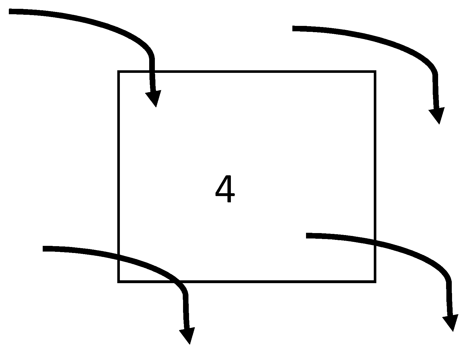
2.1. Crash Governing Equation

During a structural crash, an energetic exchange occurs between the collision systems, which causes an energy balance due to the absorption of kinetic energy, and also the loss of interatomic binding energy due to the rupture produced. In this context, the following equation, inspired by article [19], describes dynamic explicit models using the “virtual power” principle as

$$\iiint {\left\{\delta u\right\}}^T[\rho \left\{F\right\}+div\left(\stackrel{̿}{\sigma }\right)-\rho \overrightarrow{\gamma }] d\Omega =0$$

(1)

$$i,j\in \left\{\mathrm{1,2},3\right\}: \iiint \delta u_i{\displaystyle \frac{\partial {\sigma }_{ji}}{\partial x_j}}-{\displaystyle \frac{\partial }{\partial x_j}}\left[\delta u_i {\sigma }_{ji}\right]+{\displaystyle \frac{\partial }{\partial x_j}}\left[\delta u_i {\sigma }_{ji}\right]-{\displaystyle \frac{\partial \delta u_i}{\partial x_j}}{\sigma }_{ji} d\Omega =0$$

(2)

Using Gauss’ theorem:

$$\iiint {\displaystyle \frac{\partial }{\partial x_j}}[\delta u_i{\sigma }_{ji}]d\Omega =\iint \delta u_i n_{j }{\sigma }_{ji} d\mathsf{\Gamma }$$

(3)

Finally:

$$\iiint {\displaystyle \frac{\partial \delta u_i}{\partial x_j}}{\sigma }_{ji}-\rho \delta u_i\left[F_i-{\gamma }_i\right]d\Omega -\iint \delta u_i {\tau }_{i}d\mathsf{\Gamma }=0$$

(4)

where

-

$\left\{F\right\}$ denotes volume forces;

-

$\stackrel{̿}{\sigma }$ denotes the stress matrix;

-

$\rho$ denotes the density of mass;

-

$\overrightarrow{\gamma }$ is the vector of acceleration;

-

${\left\{\delta u\right\}}^T$ denotes virtual displacements;

-

$\left\{\tau \right\}=\left[\stackrel{̿}{\sigma }\right]\left\{n\right\}$ denotes the vector of stress on the boundary surface.

2.2. Strain Formulation

In structural analysis, it is crucial to distinguish between two types of deformation in order to model structures undergoing crashes more accurately.

The small strain assumes that the deformations are infinitesimal (i.e., small disturbances of the structure), and this assumption simplifies the mathematical formulation and its function in the case of linear materials.

The large strain is best adapted for extreme load conditions, such as bending, tensile force, and compression, which is critical not only for describing the crash but also for predicting significant failures.

Consequently, while small deformation models may suffice for minor impacts, large deformation models are essential for realistic and reliable crash simulations.

2.3. Strain Tensor

The gradient of displacement tensor $\stackrel{̿}{H}$ can be decomposed into two parts, one of which is deviatory symmetrical $\stackrel{̿}{\epsilon }$ and the other rotated antisymmetric $\stackrel{̿}{\omega }$:

$$\stackrel{̿}{H}=\stackrel{̿}{\epsilon }+\stackrel{̿}{\omega }$$

(5)

with

$$\left\{\begin{array}{c}\stackrel{̿}{\epsilon }={\displaystyle \frac{1}{2}}(\stackrel{̿}{H}+{\stackrel{̿}{H}}^T)\\ \stackrel{̿}{\omega }={\displaystyle \frac{1}{2}}(\stackrel{̿}{H}-{\stackrel{̿}{H}}^T)\end{array}\right.\hspace{1em}\iff \left\{\begin{array}{c}{\epsilon }_{ij}={\displaystyle \frac{1}{2}}({\displaystyle \frac{\partial u_i}{\partial x_j}}+{\displaystyle \frac{\partial u_j}{\partial x_i}})\\ {\omega }_{ij}={\displaystyle \frac{1}{2}}({\displaystyle \frac{\partial u_i}{\partial x_j}}-{\displaystyle \frac{\partial u_j}{{\partial x}_i}})\end{array}\right.$$

(6)

The gradient deformation tensor is written as a function of $\stackrel{̿}{H}$ as follows:

$$\stackrel{̿}{E}={\displaystyle \frac{1}{2}}\left(\stackrel{̿}{H}+{\stackrel{̿}{H}}^T\right)+{\displaystyle \frac{1}{2}}{\stackrel{̿}{H}}^T \stackrel{̿}{H}$$

(7)

then

$${ E}_{ij}={\displaystyle \frac{1}{2}}\left({\displaystyle \frac{\partial u_i}{{\partial x}_j}}+{\displaystyle \frac{\partial u_j}{\partial x_i}}\right)+{\displaystyle \frac{1}{2}}{\displaystyle \frac{\partial u_i}{\partial x_j}}{\displaystyle \frac{\partial u_j}{\partial x_i}}$$

(8)

2.4. Small Strain Formulation

In the case of a small strain, the norm of the tensor gradient of displacement is negligible, $‖\stackrel{̿}{H}‖$ << 1, so that

$${\displaystyle \frac{1}{2}}{\displaystyle \frac{\partial u_i}{{\partial x}_j}}{\displaystyle \frac{\partial u_j}{\partial x_i}}\to 0\Rightarrow the strain is linear$$

The formulation of small deformations relies on values derived from the initial configuration. This can be determined either at the beginning of the simulation or at the point when the small deformations begin. The strain rate is represented by

$${\dot{\epsilon }}_{i,j}={\left({\displaystyle \frac{\partial {\mathsf{\Phi }}_I}{\partial x_j}}\right)}_{t=0}{\vartheta }_{i,I}$$

(9)

with

${\mathsf{\Phi }}_I$ as the interpolating shape functions;

${\vartheta }_{i,I}$ as the components of velocity at node I.

Thus, an arbitrary strain in x direction is formulated as:

$${\epsilon }_{xx}=\sum {\dot{\epsilon }}_{xx}∆t={\displaystyle \frac{\mathsf{\Delta }x}{x_0}}$$

(10)

where x refers to the length of the part in x direction.

Thus, the stress is formulated based on the strain rate and the law of provided material, by relation integral of the internal force vector:

$$f_{iI}^{int}=\iiint {\sigma }_{ij}{\left({\displaystyle \frac{\partial {\mathsf{\Phi }}_I}{\partial x_j}}\right)}_{t=0}d{\Omega }_{elem} / i=\mathrm{1,2},3$$

(11)

where $f_{iI}^{int}$ denotes the internal vector force in the element I occupied by the volume ${\Omega }_{elem . }$

2.5. Large Strain Formulation

The large strain formulation is used with explicit time integration by calculating the derivative’s shape function for each cycle, where the special brick derivative’s function is written as

$$\left({\displaystyle \frac{\partial {\mathsf{\Phi }}_I}{\partial x_j}}\right){=\left[F\left(t\right)\right]}^{-1}\left({\displaystyle \frac{\partial {\mathsf{\Phi }}_I}{\partial r}}\right)$$

(12)

where [F(t)] is the Jacobian matrix.

As in the case of small displacement, stress is formulated by the relation integral of the internal force vector:

$$f_{iI}^{int}={\sigma }_{ij}\left({\displaystyle \frac{\partial {\mathsf{\Phi }}_I}{\partial x_i}}\right) {\Omega }_{elem}$$

(13)

The true stress time integration is expressed by

$${\sigma }_{ij}\left(t+\delta t\right)={\sigma }_{ij}\left(t\right)+{\displaystyle \frac{d{\sigma }_{ij}}{dt}} dt$$

(14)

so that the strain rate from special velocity derivatives is as follows:

$${\displaystyle \frac{d{\epsilon }_{ij}}{dt}}={\displaystyle \frac{1}{2}} \left[{\displaystyle \frac{\partial V_{ij}}{\partial x_j}}+{\displaystyle \frac{\partial V_{ji}}{\partial x_i}}\right]$$

(15)

where $V_{ij}={\displaystyle \frac{d}{dt}}{u}_{ij}$.

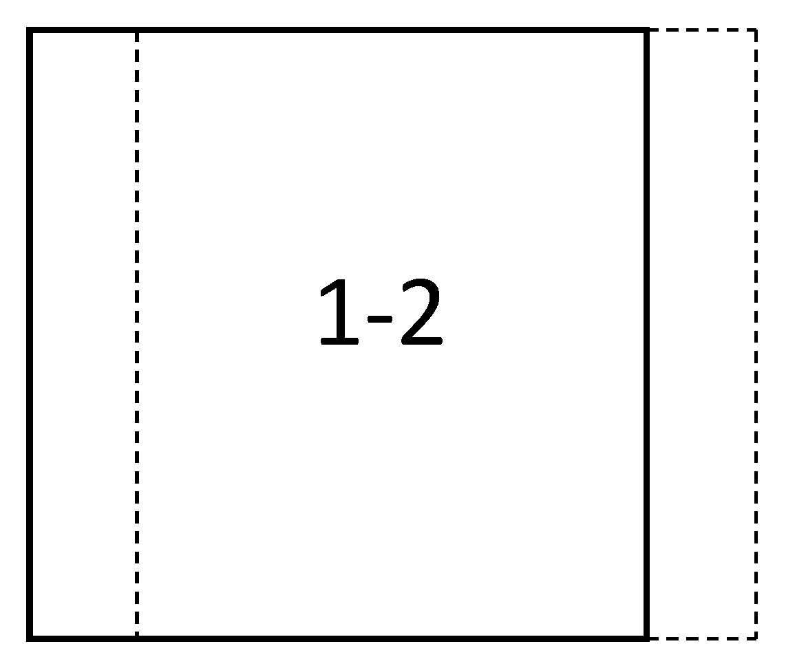
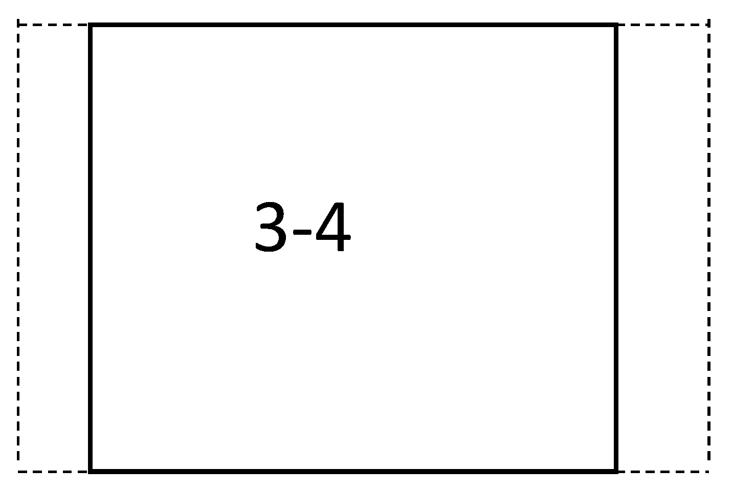
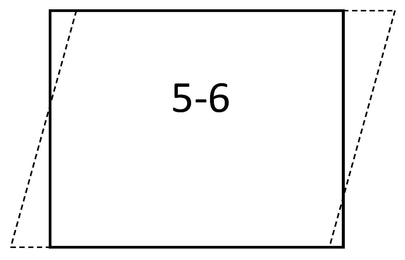
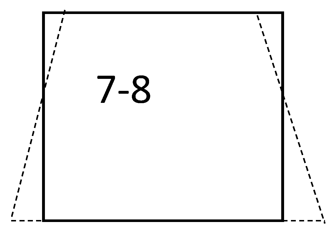
2.6. Finite Element Formulation for Crash Analysis

Finite Element Analysis is an integral numerical methodology frequently used in product life cycle development, specifically at the validation phase in objects to numerically simulate the behavior of mechanical systems after the design; it is also used for making efficient solutions based on post-processing results. Many researchers and companies that specialize in this versatile field have developed several numerical protocols to make simulations more realistic, and they have also created software that optimizes modeling organizations and sub-systems management.

The theoretical concept is to use the Lagrange basis function for interpolating displacement, temperature, and other physical state functions.

Forces generally have two kinds of distribution: internal and external forces, where the internal $f_{il}^{int}$ represents the stress in the body and is expressed by Cauchy stress:

$$f_{il}^{int}=\iiint {\sigma }_{ji}\left({\displaystyle \frac{\partial {\mathsf{\Phi }}_l}{\partial xj}}\right)d\Omega$$

(16)

Introducing a virtual displacement $\delta u_{il}$ and applying the principle of virtual power, the formula is given by

$${\delta P}^{int}=\delta u_{il}{ f}_{il}^{int}=\iiint \delta u_{il} {\sigma }_{ji}\left({\displaystyle \frac{\partial {\mathsf{\Phi }}_l}{\partial xj}}\right)d\Omega$$

(17)

The external forces present the multiplication of weight and the acceleration. Similar to the internal virtual power, the external force is expressed by

$${\delta P}^{ext}=\delta u_{il}{ f}_{il}^{ext}=\iiint \delta u_{il} {\mathsf{\Phi }}_l \rho F_{i}d\Omega +\iint \delta u_{il} {\mathsf{\Phi }}_l \dot{{\tau }_i} d\mathsf{\Gamma }$$

(18)

In numerical simulation, it is essential to transform and update the coordinates, enabling the geometric and physical properties to be calculated with great precision. In this field, the Jacobian matrix J plays the role of mapping between real-space coordinates and intrinsic coordinates, describing the rate of change of the linear transformation application so that it is bijective between physical space and parameter space, playing the role of changing variables for calculating integrals. The following integral describes how the Jacobian matrix helps to solve integrals with facility and flexibility so as to be programmable:

$$\underset{\Omega }{\int }f\left(x\right)d\Omega =\underset{{\Omega }^0}{\int }f\left(x\right)\left|J\right|d{\Omega }^0=\underset{∆}{\int }f\left(\mathsf{\xi }\right)\left|J_{\mathsf{\xi }}\right|d∆$$

(19)

where

-

$\left|J\right|$ denotes the determinant of the transformation between the current and the initial configuration;

-

${\Omega }^0$ denotes the intrinsic configuration;

-

$\Omega$ denotes the physical configuration;

-

$\left|J_{\mathsf{\xi }}\right|$ denotes the determinant of the transformation between the current configuration and the domain in the intrinsic coordinate system.

In addition, the Jacobian matrix is described as

$$J_{\mathsf{\xi }\mathrm{k}\mathrm{j}}={\displaystyle \frac{\partial x_k}{\partial {\mathsf{\xi }}_j}}$$

(20)

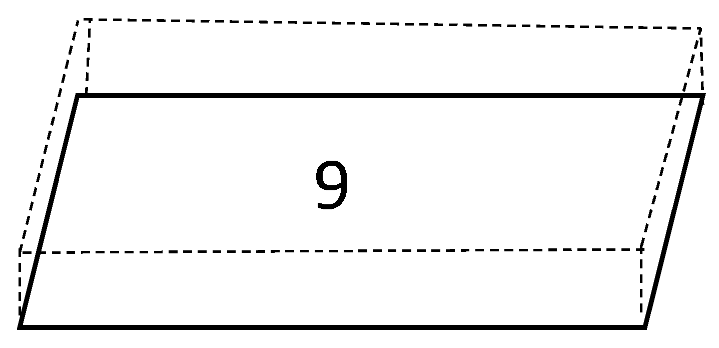
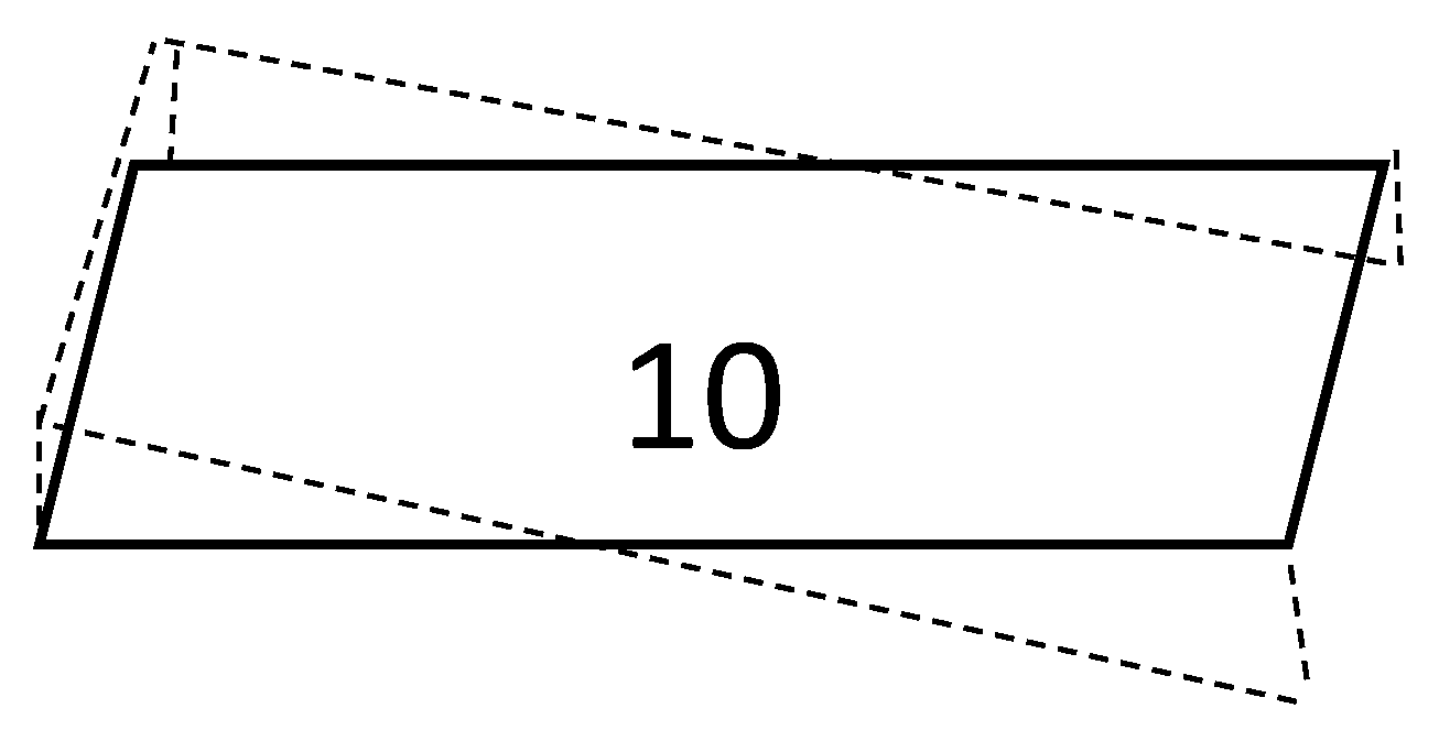
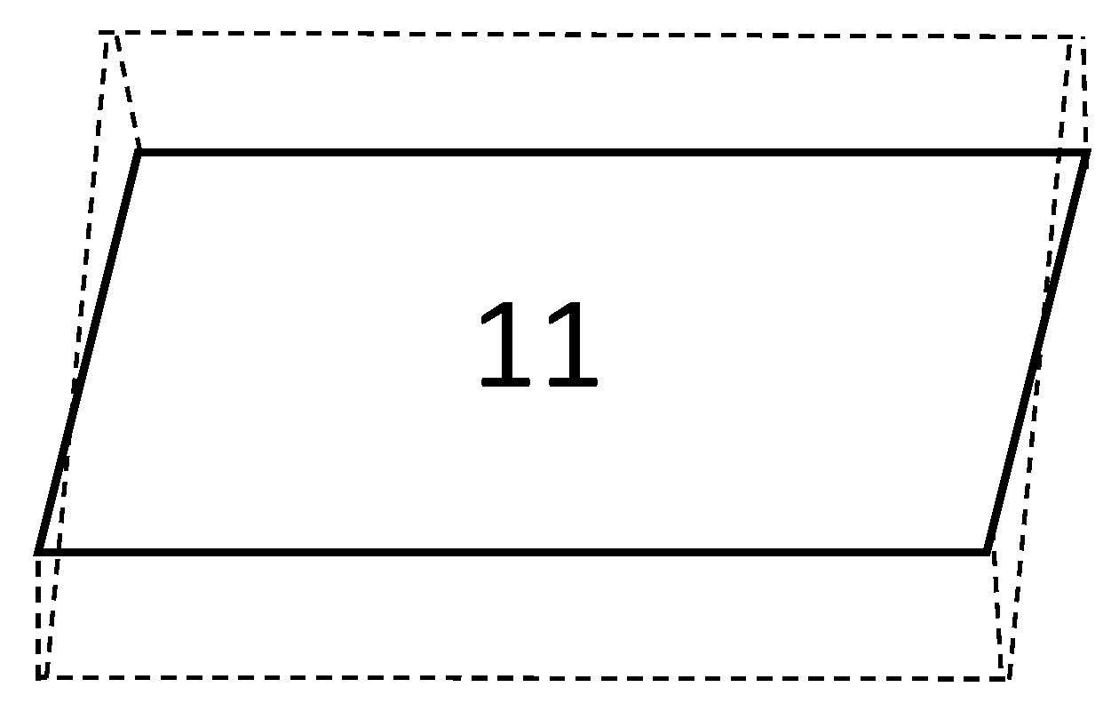
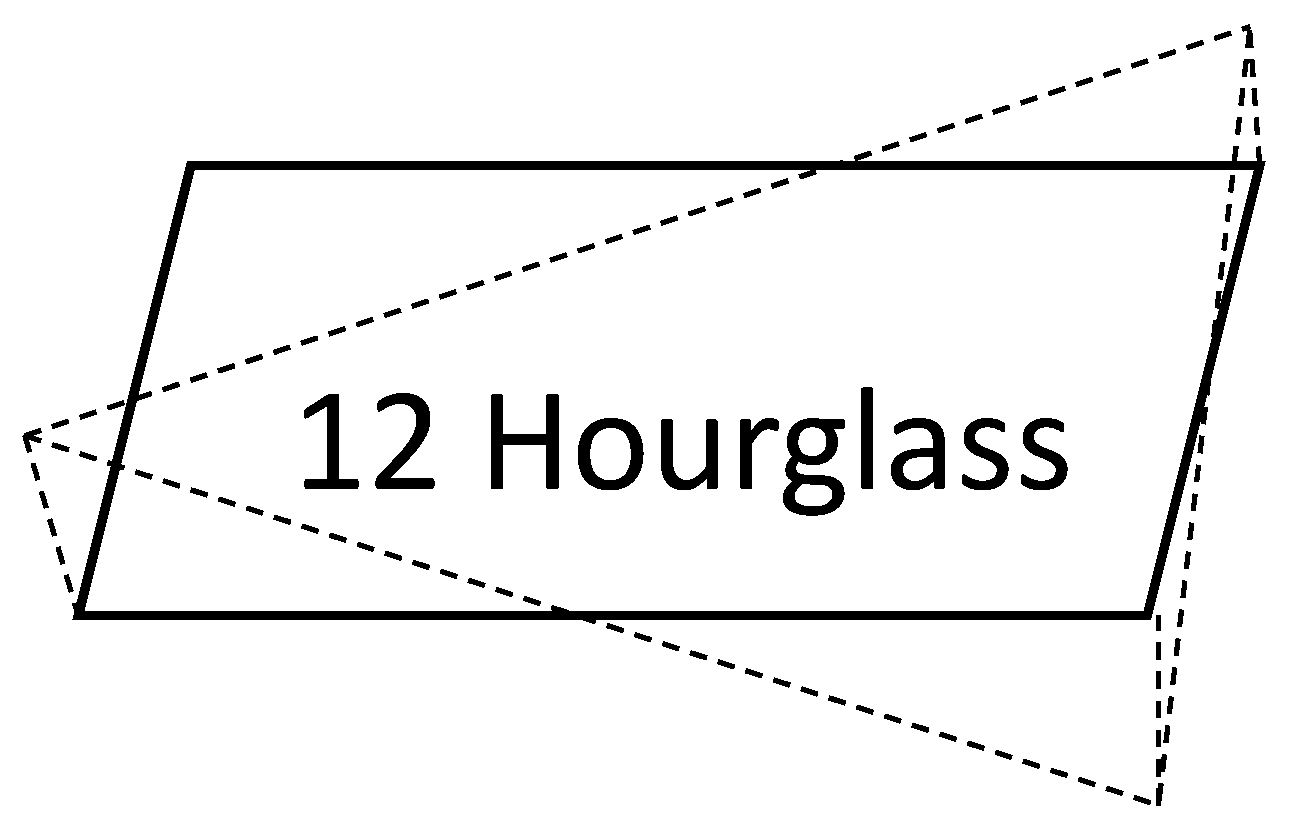
2.7. Hourglass and Technical Solutions

The hourglass mode describes elements with zero strain energy, with this phenomenon coming from the distortion of those elements, where there is no stress applied on the nodes. Researchers have distinguished 12 different modes of break, dispatched by four for each of the three coordinate systems; the following figures contain the mode of distortion of elements in translation, describing two modes of shell hourglass, namely modes 7, 8 and 12, referring to the Radioss Altair standard nomination (see Figure 1, Figure 2, Figure 3, Figure 4, Figure 5, Figure 6, Figure 7 and Figure 8):

In addition to the translational modes, the 4-node shell features 12 rotational modes: four modes for out-of-plane rotations (1 through 4), two deformation modes (5 and 6), two modes that combine rigid body and deformation (7 and 8), and four hourglass modes (9 through 12) (see Figure 9, Figure 10, Figure 11, Figure 12, Figure 13, Figure 14, Figure 15 and Figure 16). The following figures show the rotational modes of deformation:

Three hourglass correction methods are available in Radioss, where plasticity is considered in computing the anti-hourglass forces. The method recommended by [20] and utilized in this work is one of these. Hourglassing is not a concern when using multiple elements (at least four through the thickness) in a 3D element configuration. Each element captures either compressive or tensile axial strains, but not both, ensuring the accurate measurement of axial strains while the thickness and shear strains remain at zero. This approach is both inexpensive and effective.

2.8. Dynamic Explicit Modeling and Newmark’s Method

Practically speaking, in FEA, there are two methods of dynamic equilibrium governing equations: the direct integration method and the superposition’s mode. The two techniques are closely related, and the selection between the two depends on the numerical effectiveness.

Direct integration involves directly integrating the equations of motion using a step-by-step numerical procedure. In this approach, the equations are not transformed into another basis. The formulation of the dynamic equilibrium equation at discrete moments incorporates the influence of inertial and damping forces. It is assumed that displacements, velocities and accelerations vary at each time interval Δt. Since a step-by-step procedure is used to obtain the solution, the various non-linearities of the system, such as geometric, material, contact and large deformation non-linearities, are naturally taken into account, even if the resolution at each step remains linear.

In general, the mode superposition method involves converting the equilibrium equation into ordinary displacement modes. An eigenvalue problem is solved. The free vibration mode shapes of the finite element assembly are called eigenvectors, and the global response is obtained by superimposing the response of each eigenvector. Since the method is based on the superposition rule, the linear response of the dynamically loaded structure as generally developed is considered, even if the resolution at each stage remains linear.

One of the most common one-step integration methods used in dynamic explicit modelling is called Newmark’s methodology, where the state of the system is computed at a given time $t_{i+1}=t_i+h$ using Taylor’s formula:

$$f\left(t_{i+1}+h\right)=f\left(t_i\right)+h{f}^{\prime }\left(t_i\right)+{\displaystyle \frac{h^2}{2}}{f}^{″}\left(t_i\right)+{\displaystyle \frac{h^3}{3!}}{f}^{\left(3\right)}\left(t_i\right)+\cdots +{\displaystyle \frac{h^s}{S!}}{f}^{\left(s\right)}\left(t_i\right)+R_s(h)$$

(21)

with

$$R_s\left(h\right)={\int }_{t_i}^{t_{i+1}}{\displaystyle \frac{1}{S!}}{f}^{\left(s+1\right)}\left(\mathsf{\tau }\right)[t_{i+1}+h-\tau {]}^{s}d\tau$$

(22)

The preceding formula allows the computation of displacements and velocities of the system at time $t_{i+1}$:

$${\dot{u}}_{i+1}={\dot{u}}_i+{\int }_{t_i}^{t_{i+1}}\ddot{u}\left(\mathsf{\tau }\right)d\mathsf{\tau }$$

(23)

$$u_{i+1}=u_i+h{\dot{u}}_i+{\int }_{t_i}^{t_{i+1}}\left(t_{i+1}-\tau \right) \ddot{u}\left(\mathsf{\tau }\right)d\mathsf{\tau }$$

(24)

The approximation consists of computing the integrals for acceleration by numerical quadrature:

$${\int }_{t_i}^{t_{i+1}}\ddot{u}\left(\mathsf{\tau }\right)d\mathsf{\tau }=\left(1-\gamma \right)h{\ddot{u}}_i+\gamma h{\ddot{u}}_{i+1}+r_n$$

(25)

$${\int }_{t_i}^{t_{i+1}}\left(t_{i+1}-\tau \right) \ddot{u}\left(\mathsf{\tau }\right)d\mathsf{\tau }=({\displaystyle \frac{1}{2}}-\beta )h^2{\ddot{u}}_i+\beta h^2{\ddot{u}}_{i+1}+{\dot{r}}_n$$

(26)

Different algorithms can be derived based on the values of γ and β: γ = 0, β = 0: pure explicit algorithm. It is demonstrable that it is inherently unstable. If a critical time step exists, an integration scheme is stable if a limited perturbation at a particular time does not result in a growing modification at subsequent time steps for a value of the time step below, or equal to, this critical value. The central difference algorithm is γ = 1/2, β = 0. Its conditional stability can be demonstrated by the Fox–Goodwin algorithm: γ = 1/2, β = 1/2. For acceleration that is linear, γ = 1/2, β = 1/6. For mean acceleration, γ = 1/2, β = 1/4. The maximally accurate method that is unconditionally stable is this integration scheme (Figure 17):

3. CFRP Materials and Chang Criteria

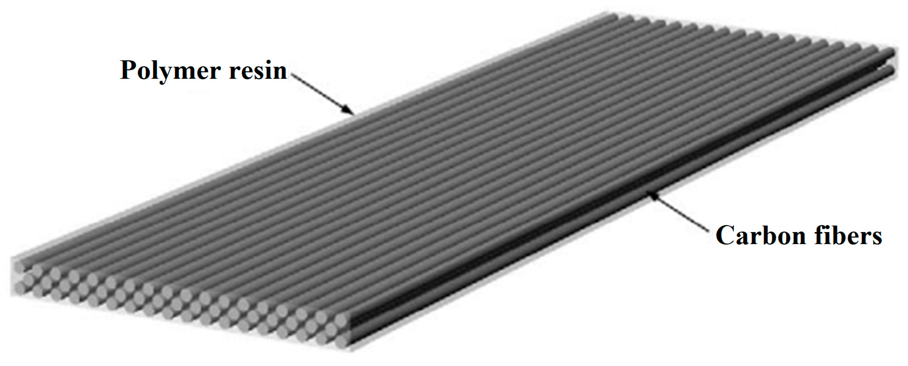
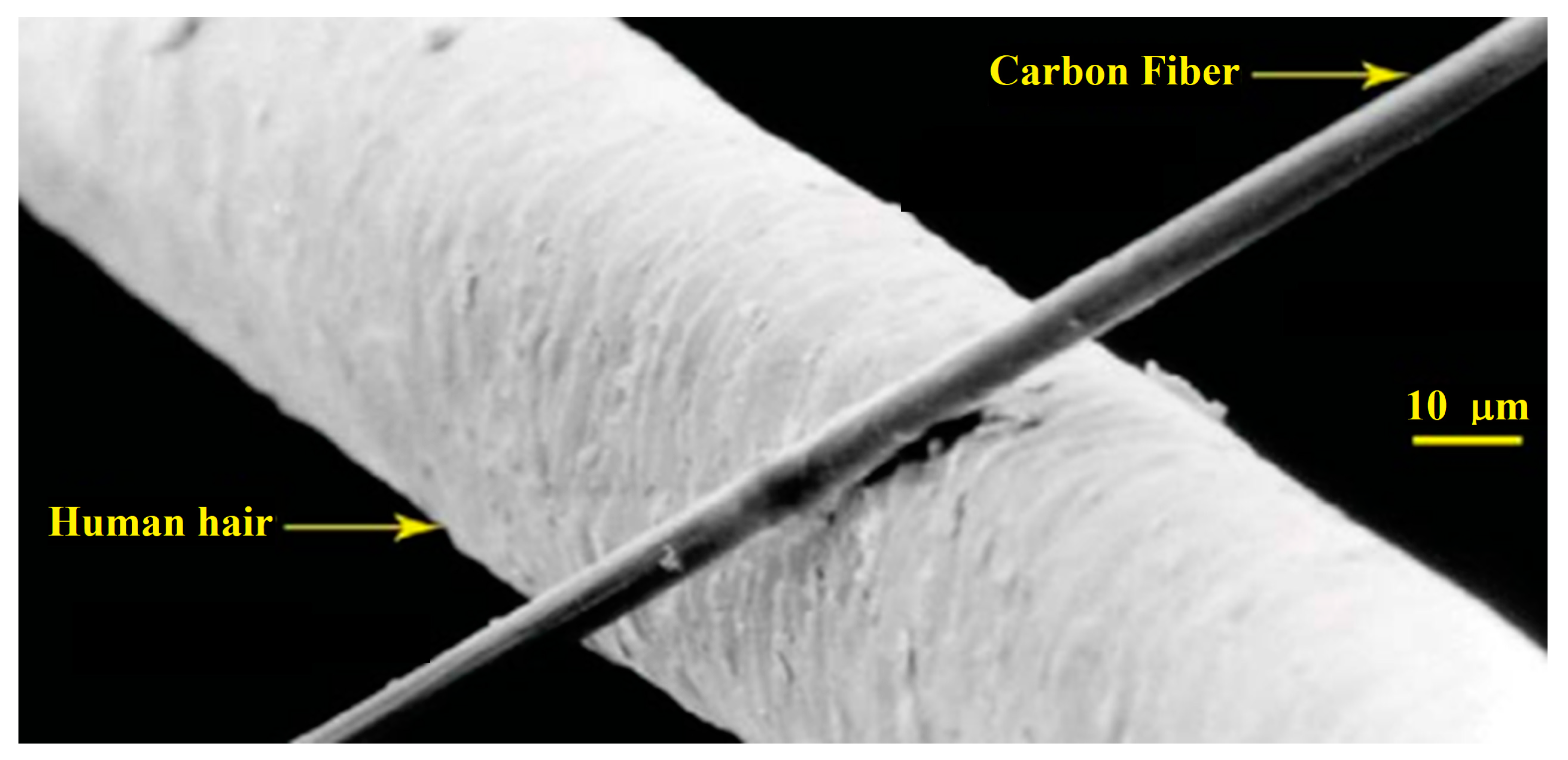
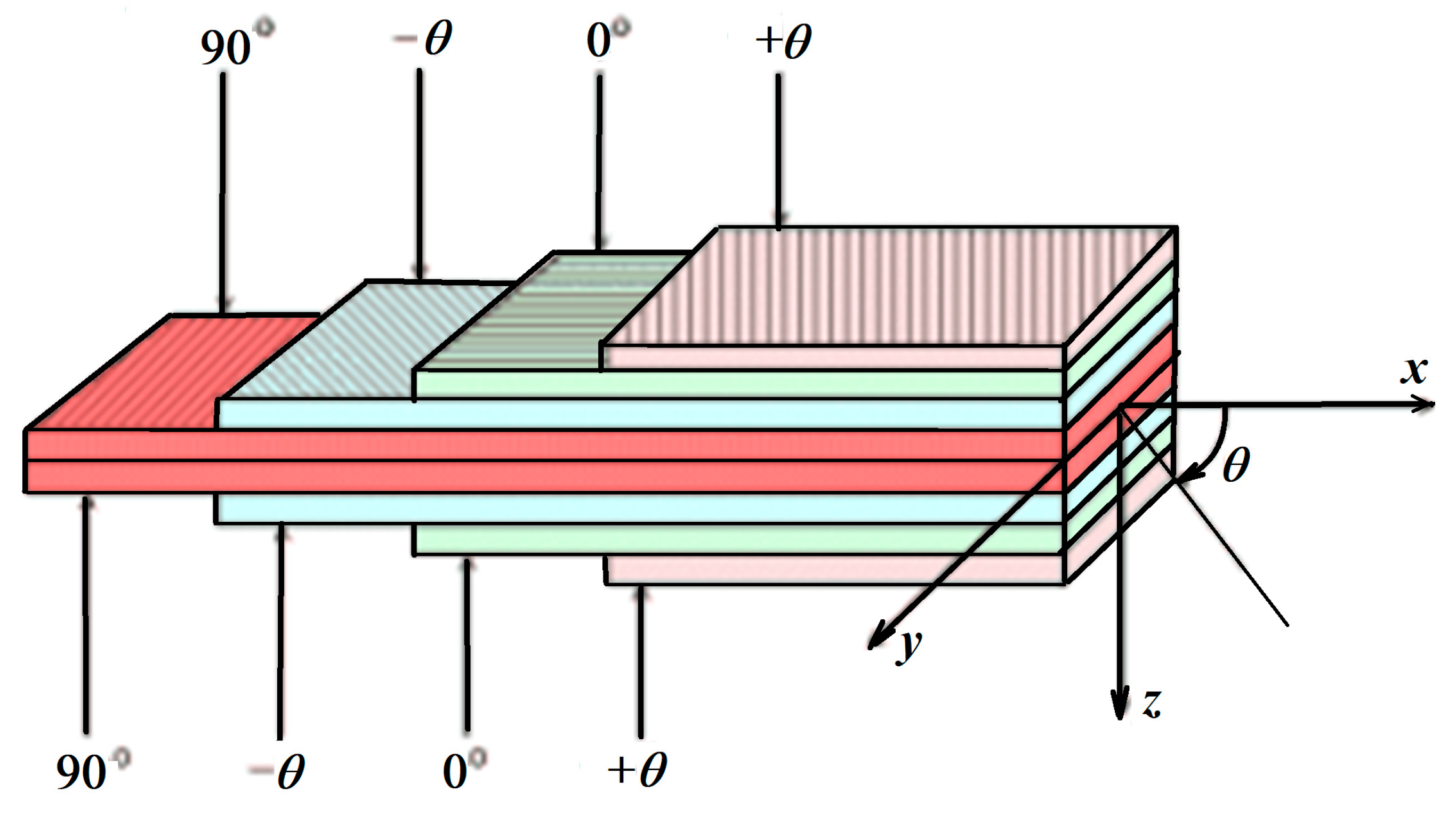
3.1. CFRP Materials

As the name suggests, the constitutions of carbon fiber reinforced polymer are carbon fibers enforcing polymer resin, where the polymer resin functions as the matrix that holds the carbon fibers [21].

Referring to [21], “carbon fibers” are defined as fibers (Figure 18) that have a minimum of 90% and a maximum of 100% carbon content. Polymeric precursor materials, including polyacrylonitrile (PAN), cellulose, pitch, and polyvinyl chloride, can be used to create the fibers. These precursors undergo a sequence of heating and tensioning treatments to become carbon fibers. When viewed in a larger context, carbon fibers are tiny filaments that are barely perceptible to the human eye, measuring between 5 and 10 μm in diameter (Figure 19). A carbon fiber’s size is likened to that of a human hair.

CFRPs can be woven, with fibers oriented in multiple directions, or they can be aligned in a single direction to create a unidirectional (UD) composite. These common composite materials consist of one or more fiber plies, such as carbon, glass, Kevlar or aramid stacked together with a resin matrix, such as epoxy, which acts as an adhesive and helps distribute the loads among the fibers. To provide the laminate with varying strengths and stiffnesses in different directions, layers with different material orientations are incorporated.

One type of composite material is CFRP, which possesses key attributes such as being lightweight and having low density, high stiffness, high strength, and good environmental properties. Having resistance to unauthorized access during crashes is vital. CFRPs are typically woven, like fabric, with fibers bonded by a resin matrix. To enhance strength and reduce brittleness, they consist of multiple layered fiber plies. Sometimes, a core material such as foam, wood or honeycomb is added between the plies to improve the composite’s strength-to-weight ratio, as seen in an I-beam where the core acts as the shear web and the laminate skins form the flange. Additionally, the ratios of fiber and matrix materials can vary based on processing techniques, significantly affecting the mechanical properties and behaviors under load.

3.2. Stress and Strain Curves

Any material used in construction must be able to endure four primary direct loads. Tension relies heavily on the following:

-

The tensile stiffness and strength of the reinforcement fibers are significantly higher than those of the resin system by itself.

-

The compression, adhesion and stiffness of the resin are essential, as the resin prevents the fiber from buckling and preserves its straight columnar shape.

-

The shear is primarily managed by the resin, which disperses stresses throughout the composite.

-

Flexure results from the combination of shear, compression and tensile loads, with the laminate experiencing shear in its middle portion, tension on its bottom face and compression on its upper face.

The choice of the matrix and fibers used is critical to the composite’s overall performance and properties (Figure 20). Along with their proportion and arrangement within the composite, these elements define its qualities. The stiffness characteristics of the ply, or lamina, are determined by the fiber fraction. A laminate consists of stacks of laminas, each with fibers that are oriented differently.

Referring to [22], the following example shows that the stress–strain curves of CFRP materials have a diagram that typically behaves almost linearly, followed by nonlinear plastic behavior (Figure 21).

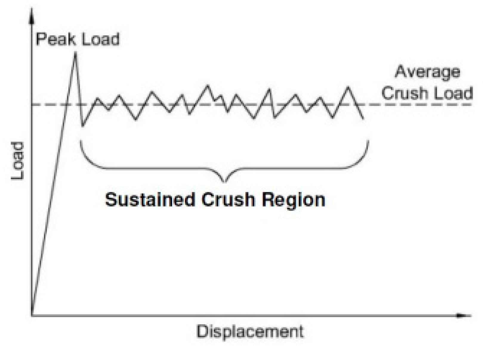
3.3. Specific Energy Absorption

The energy that is absorbed is a key attribute for assessing crashworthiness. A crushing event usually starts with a rapidly increasing force until it reaches the maximum, or peak, compressive load. The desired post-peak performance, known as progressive crushing, is marked by a relatively stable load that is generally lower than the peak load. The force-versus-displacement graph generated during this process reflects this gradual crushing behavior (Figure 22) [6].

The SEA is defined as the energy absorbed per crashed mass and is expressed as [15]

$$SEA={\displaystyle \frac{W}{\rho A\delta }}={\displaystyle \frac{\int Fd\delta }{\rho A\delta }}$$

(27)

where W denotes the mechanical work during crashing, F refers to the applied forces, $\rho$ is the density volume of mass, A refers to the area of the section studied and $\delta$ describes the displacement.

3.4. Damage Initiation and Propagation

CFRP materials are generally characterized by brittle damage initiated without large deformations because the plasticity is not taken into account when modelling the behavior of those materials [23,24,25,26].

According to orthotropic material stress–strain behavior [27], the relation of the compliance is defined as

$$\sigma =H\epsilon$$

(28)

where

$$H={\displaystyle \frac{1}{D}}\left[\begin{array}{ccc}(1-{\mathrm{d}}_1){\mathrm{E}}_1& (1-{\mathrm{d}}_1)(1-{\mathrm{d}}_2){\mathsf{\nu }}_{21}{\mathrm{E}}_2& 0\\ (1-{\mathrm{d}}_1)(1-{\mathrm{d}}_2){\mathsf{\nu }}_{21}{\mathrm{E}}_2& (1-{\mathrm{d}}_2){\mathrm{E}}_2& 0\\ 0& 0& D(1-{\mathrm{d}}_{12)}{\mathrm{G}}_{12}\end{array}\right]$$

(29)

where D = 1 −$(1-{\mathrm{d}}_1)(1-{\mathrm{d}}_2){\mathsf{\nu }}_{21}{\mathsf{\nu }}_{12}$; ${\mathrm{E}}_1$ and ${\mathrm{E}}_2$ are the Young’s modulus in the principal directions; ${\mathrm{G}}_{12}$ is the shear modulus; ${\mathsf{\nu }}_{12}$ and ${\mathsf{\nu }}_{21}$ are Poisson’s ratios; ${\mathrm{d}}_1$ and ${\mathrm{d}}_2$ reflect the principal state of damage; and ${\mathrm{d}}_{12}$ the damage parameter is linked to micro-cracking in the matrix caused by in-plane shear deformation.

The damage variables, ${\mathrm{d}}_{1+}$ and ${\mathrm{d}}_{1-}$, are associated with tensile and compressive fiber failure, whereas the ${\mathrm{d}}_{2+}$ and ${\mathrm{d}}_{2-}$ damage parameters are associated with the transverse direction cracking due to tensile and compressive load. The shear damage parameter, ${\mathrm{d}}_{12}$, is influenced by longitudinal and transverse cracks, and it is defined as

$${\mathrm{d}}_{\mathrm{i}}={\mathrm{d}}_{\mathrm{i}+}{\displaystyle \frac{<{\mathsf{\sigma }}_{\mathrm{i}}>}{\left|{\mathsf{\sigma }}_{\mathrm{i}}\right|}}+{\mathrm{d}}_{\mathrm{i}-}{\displaystyle \frac{<{-\mathsf{\sigma }}_{\mathrm{i}}>}{\left|{\mathsf{\sigma }}_{\mathrm{i}}\right|}}$$

(30)

$${\mathrm{d}}_{12}=1-(1-{\mathrm{d}}_{1+})(1-{\mathrm{d}}_{1-})(1-{\mathrm{d}}_{2+})(1-{\mathrm{d}}_{2-})$$

(31)

3.5. Chang Failure Criteria

Many studies use the Chang criteria, with a matrix damage threshold that differs noticeably from the Hashin criterion, to forecast the low-velocity impact of composite materials. However, the impact of three failure criteria on the mechanical response and damage distribution of composite laminates under a low-velocity impact has not been thoroughly compared in the relevant research [28].

Where direction one refers to the fiber direction, the failure criteria for fiber breakage is written as follows:

-

Tensile fiber mode: ${\sigma }_{11}$ > 0:

$$e_f^2={\left({\displaystyle \frac{{\sigma }_{11}}{{{\sigma }_1}^c}}\right)}^2+\mathsf{\beta }{\left({\displaystyle \frac{{\sigma }_{12}}{{\overline{\sigma }}_{12}}}\right)}^2$$

(32)

-

Compressive fiber mode: ${\sigma }_{11}$ < 0:

$$e_c^2={\left({\displaystyle \frac{{\sigma }_{11}}{{{\sigma }_1}^c}}\right)}^2$$

(33)

-

For matrix cracking, the failure criteria are as follows:

• Tensile matrix mode ${\sigma }_{22}$ > 0:

$$e_m^2={\left({\displaystyle \frac{{\sigma }_{22}}{{{\sigma }_2}^t}}\right)}^2+\mathsf{\beta }{\left({\displaystyle \frac{{\sigma }_{12}}{{\overline{\sigma }}_{12}}}\right)}^2$$

(34)

• Compressive matrix mode ${\sigma }_{22}$ < 0:

$$e_d^2={\left({\displaystyle \frac{{\sigma }_{22}}{2{\overline{\sigma }}_{12}}}\right)}^2+\left[{\left({\displaystyle \frac{e_c^2}{2{\overline{\sigma }}_{12}}}\right)}^2-1\right]{\displaystyle \frac{{\sigma }_{22}}{{{\sigma }_2}^c}}+{\left({\displaystyle \frac{{\sigma }_{12}}{{\overline{\sigma }}_{12}}}\right)}^2$$

(35)

where

-

${{\sigma }_1}^c,{{\sigma }_1}^t$ are fiber compressive/fiber tensile;

-

${{\sigma }_2}^c,{{\sigma }_2}^t$ are compressive and tensile loading in direction 2;

-

${\overline{\sigma }}_{12}$ is shear strength in composite ply plane;

-

$\mathsf{\beta }$ is the shear scale factor, which can be determined experimentally.

This damage value, D, is expressed as

$$\mathrm{D}=\mathrm{Max} (e_f^2,e_c^2,e_m^2,e_d^2)$$

where the element of structure is

• Non-failure, if 0 ≤ D < 1;
• Failure, if D = 1.

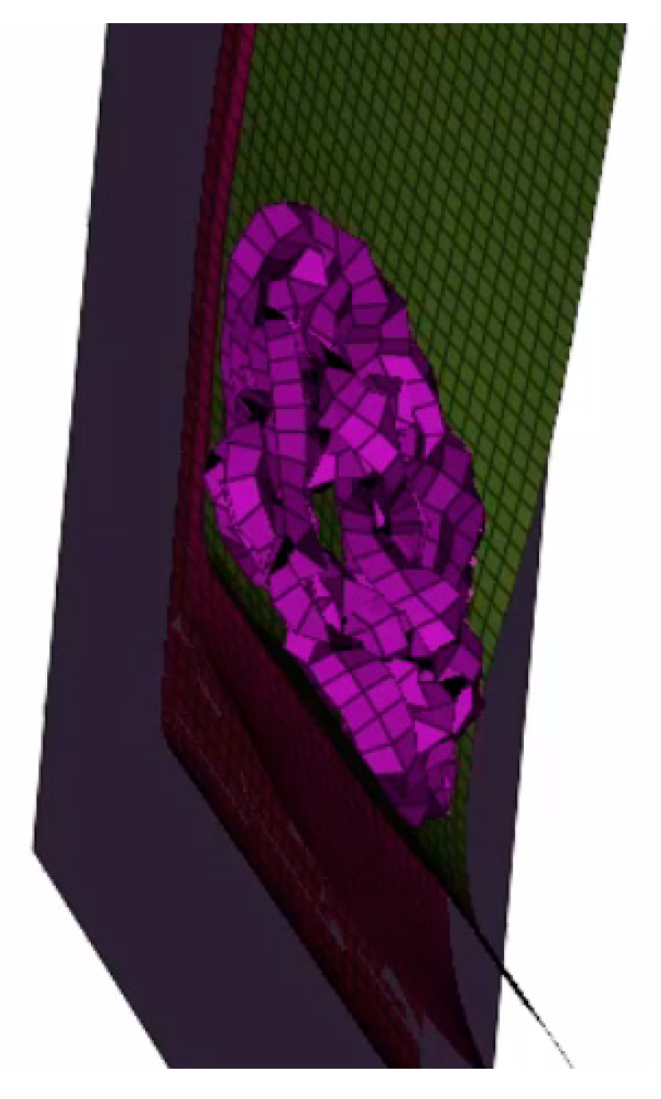
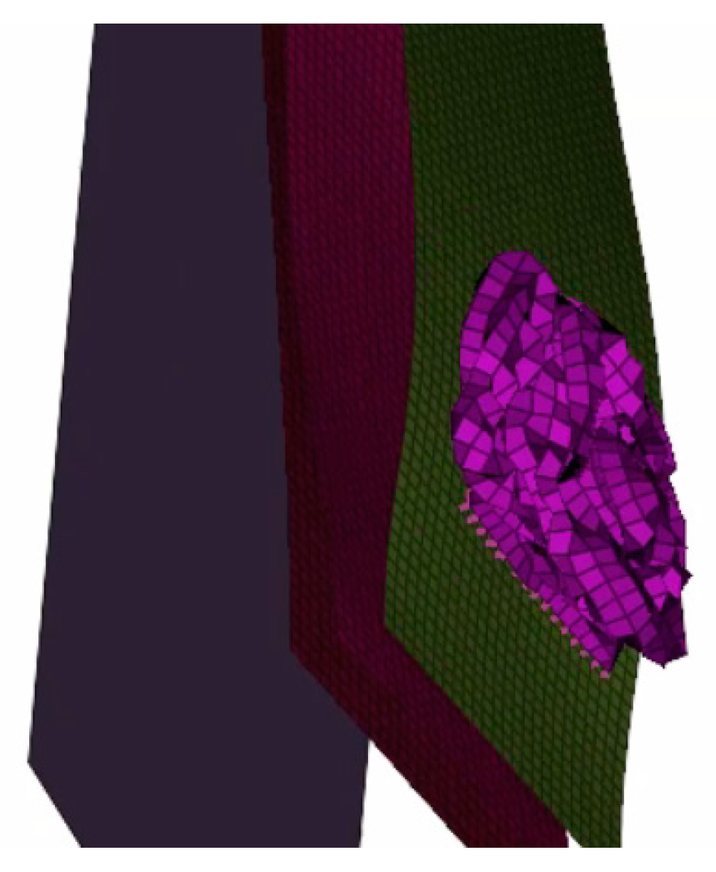
4. Numerical Simulation and Discussion

Many automotive manufacturers have endeavored to make calculations more efficient and realistic because of the difference between the animations and the physical values. The Johnson–Cook and GISSMO failures are examples that are frequently used in the case of metallic material [29]. This study has developed a model combining the LAW 25 [30] and the Chang failure criteria to correct the behavior of animations to be coherent with kinetic physical parameters.

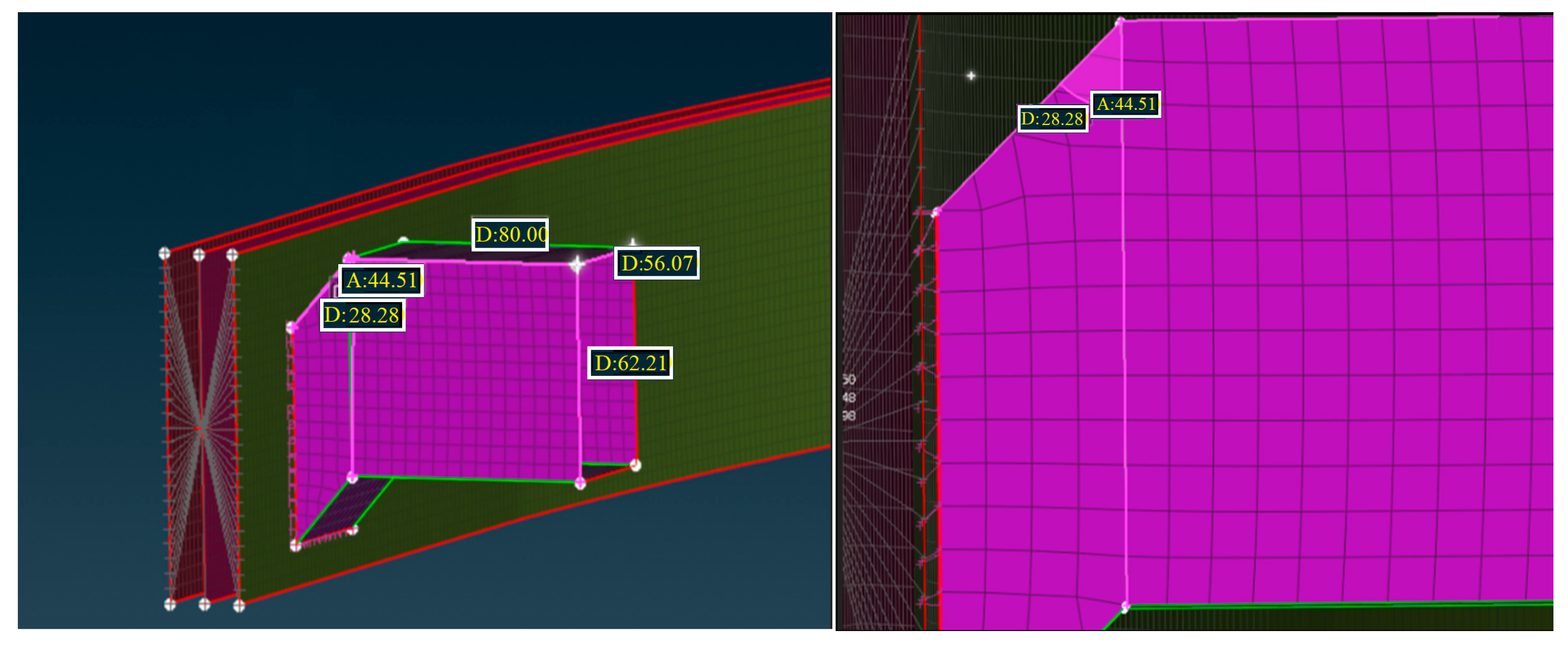
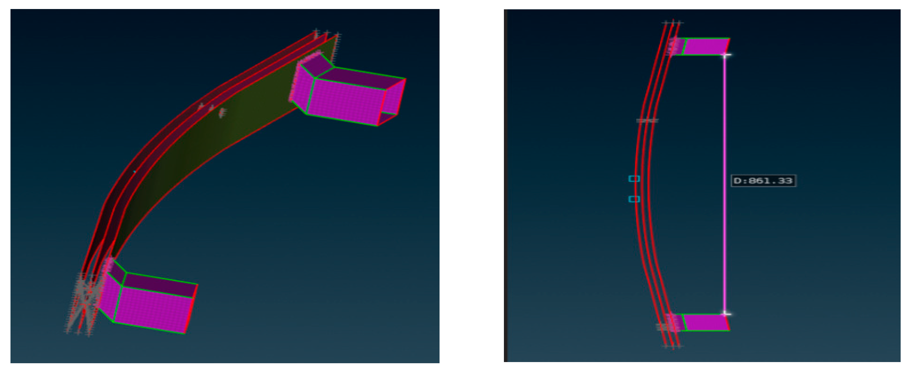
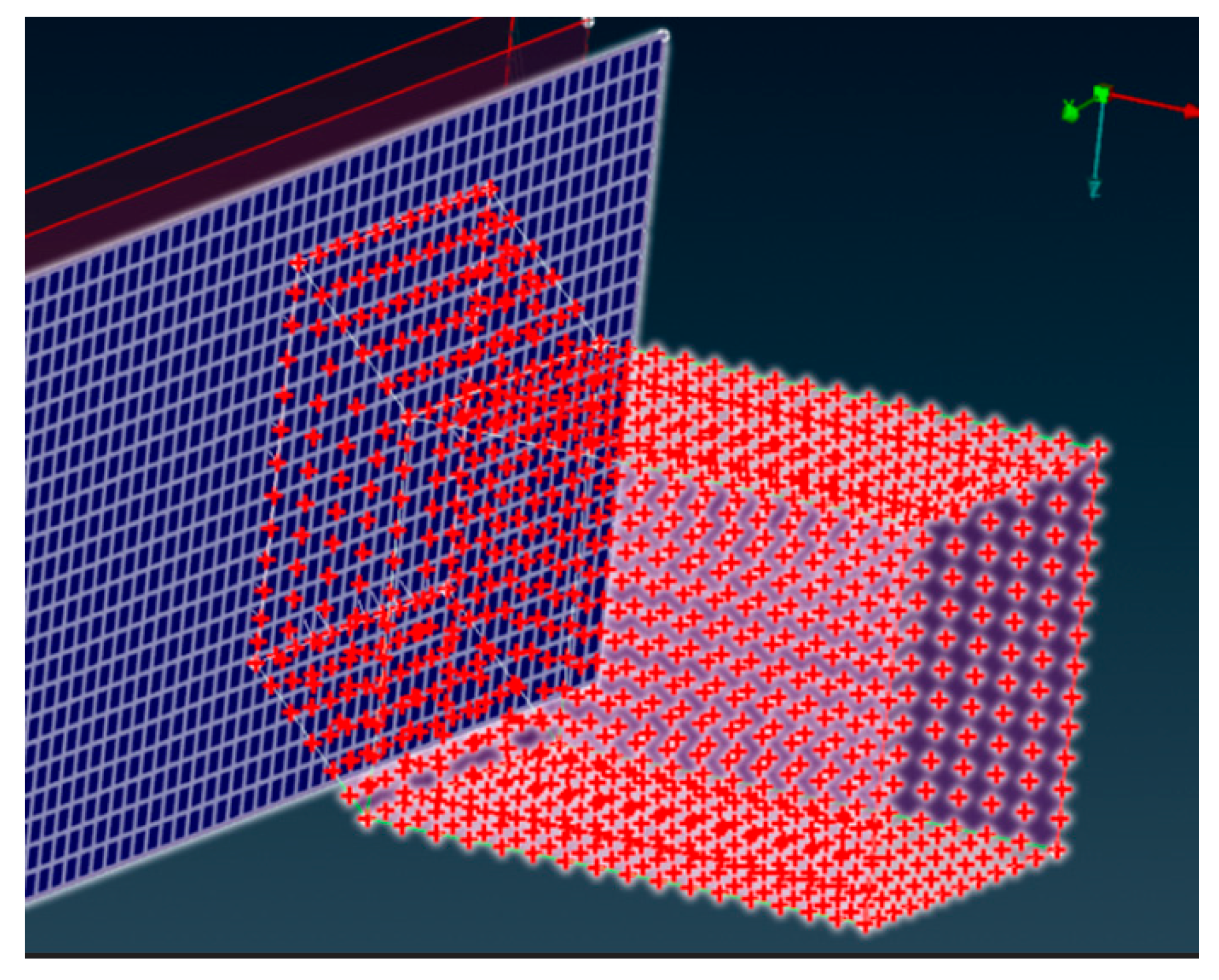
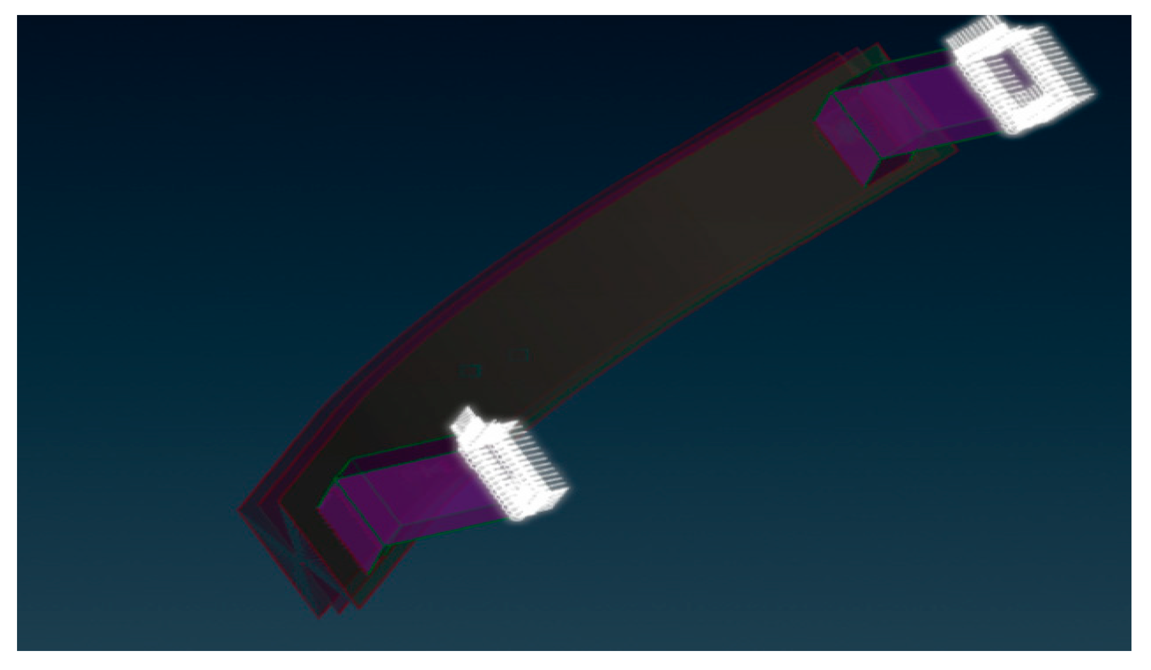
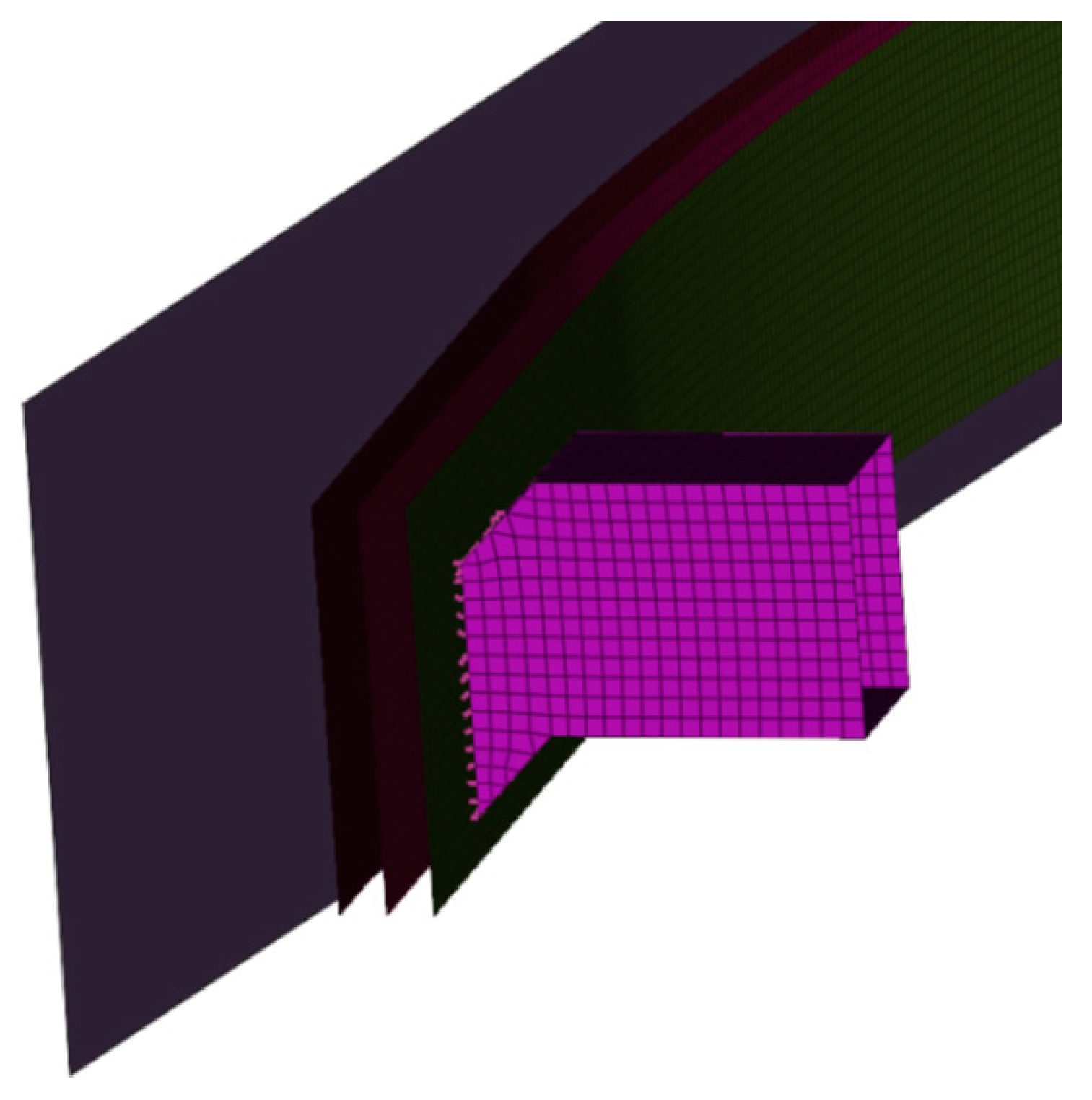
4.1. Geometry and the Material’s Input Data

In this study, a crash box made of CFRP material was used to compare two case studies of an object to optimize the simulation of a crash using this kind of material.

The upper figure represents the studied geometry with QUAD mesh elements dedicated for composite shell property respecting the Altair standard (Size: 5 mm × 5 mm), with a symmetrical representation of the left and right crash box (Figure 23 and Figure 24), connected with a bar using the Radioss spring element implemented in ANSA CAE, as well as a T7 contact to avoid intersection after the load’s application (Figure 25).

Based on standard material databases, the following table describes the material used for this study in an object to be used as a kind of brittle elastic CFRP material and to illustrate the paper’s perspective in comparing the result of kinetic energy with [31] in case of the application of Chang failure, without this failure model, and regarding different behaviors (see

Table 1. CFRP material property used for the study (SAE J2630).

Material’s Property	Values
Young’s modulus longitudinal direction	56,275 MPa
Young’s modulus transverse direction	54,868 MPa
Shear modulus	4211 MPa
Density	1.52 × ${10}^{-6}$ kg/${\mathrm{m}\mathrm{m}}^3$
Longitudinal compressive strength	570 MPa
Transverse compressive strength	355 MPa
Longitudinal tensile strength	917.38 MPa
Transverse tensile strength	775.38 MPa
Shear strength	132.5 MPa

).

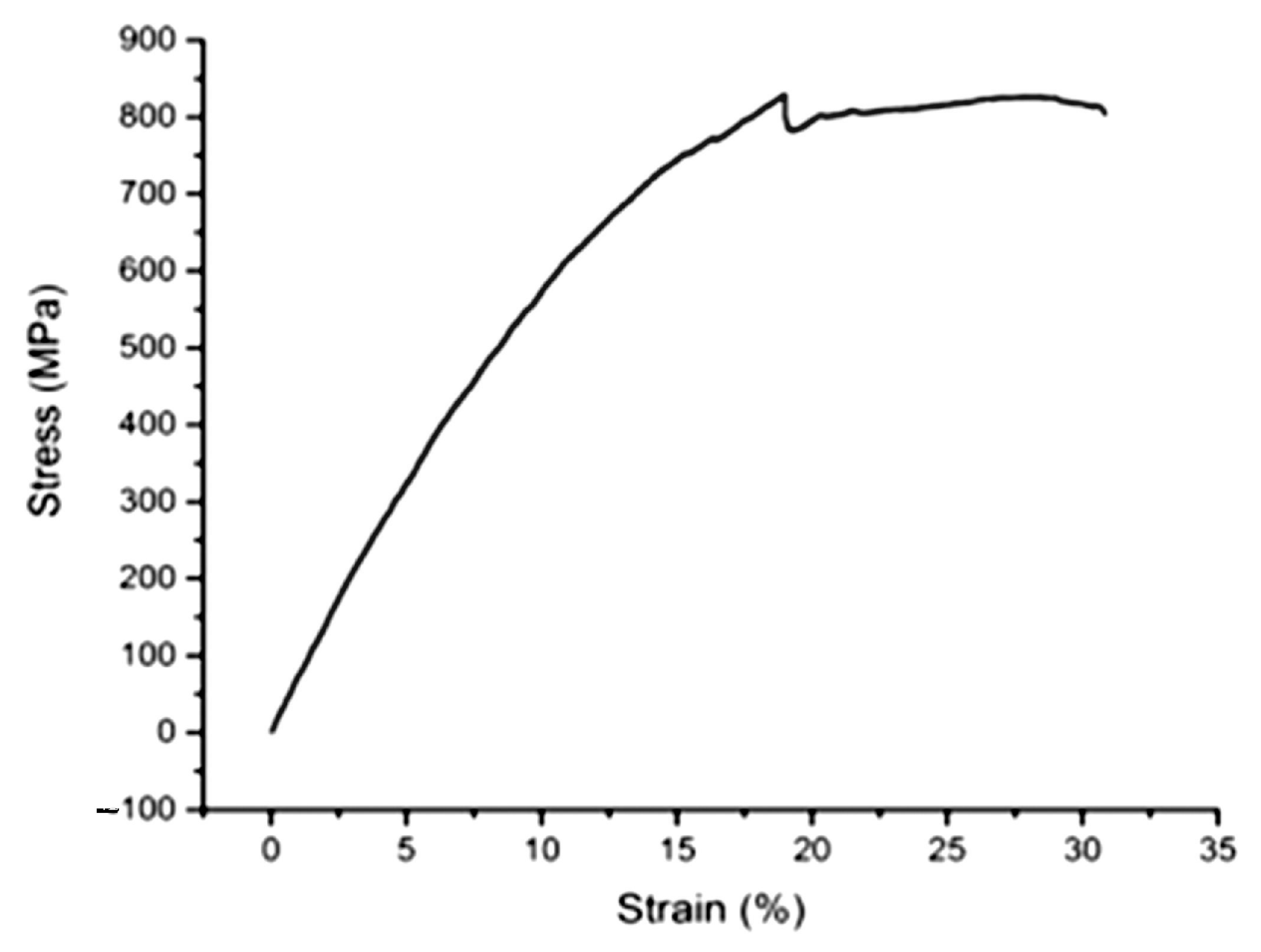
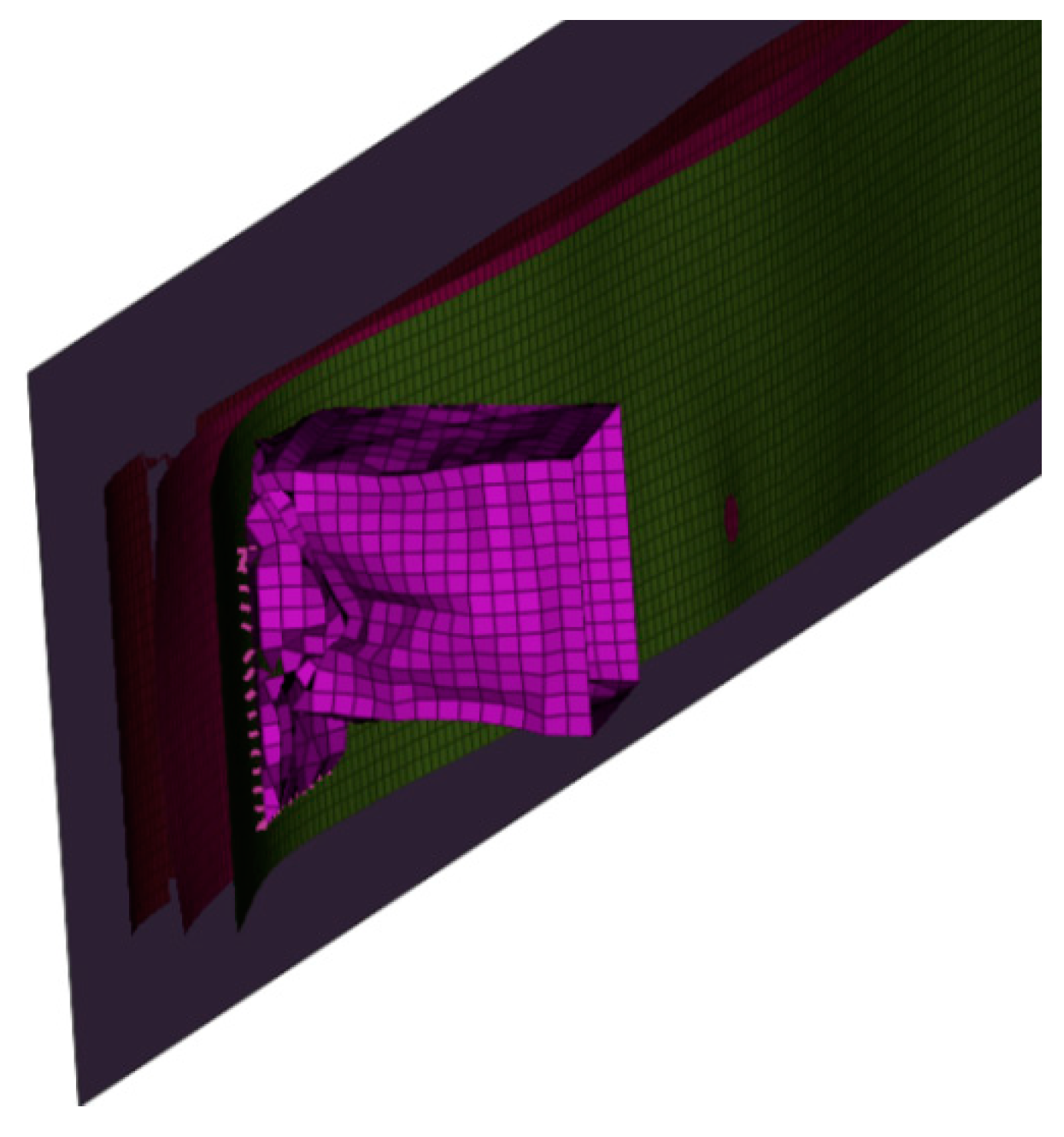
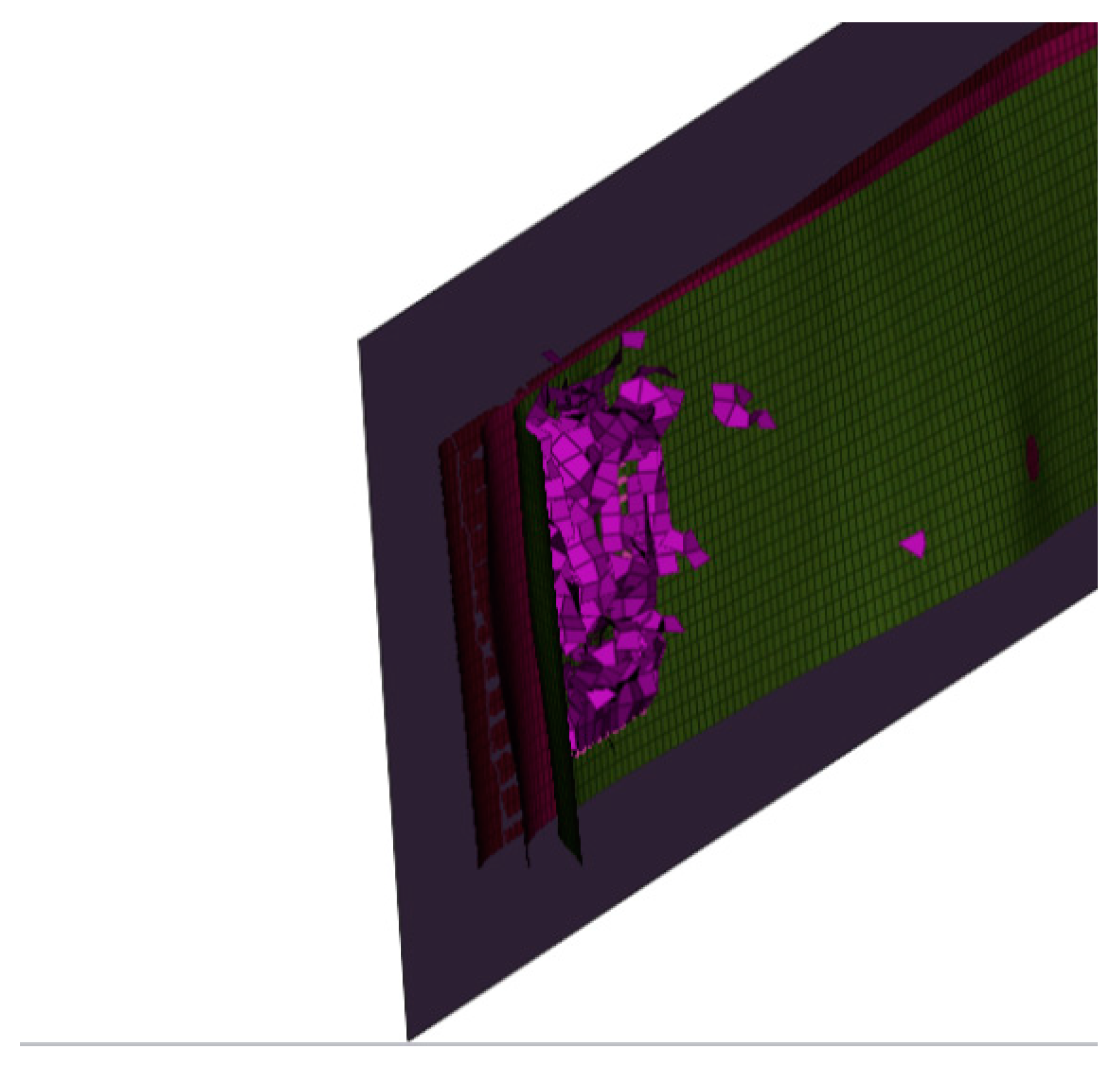
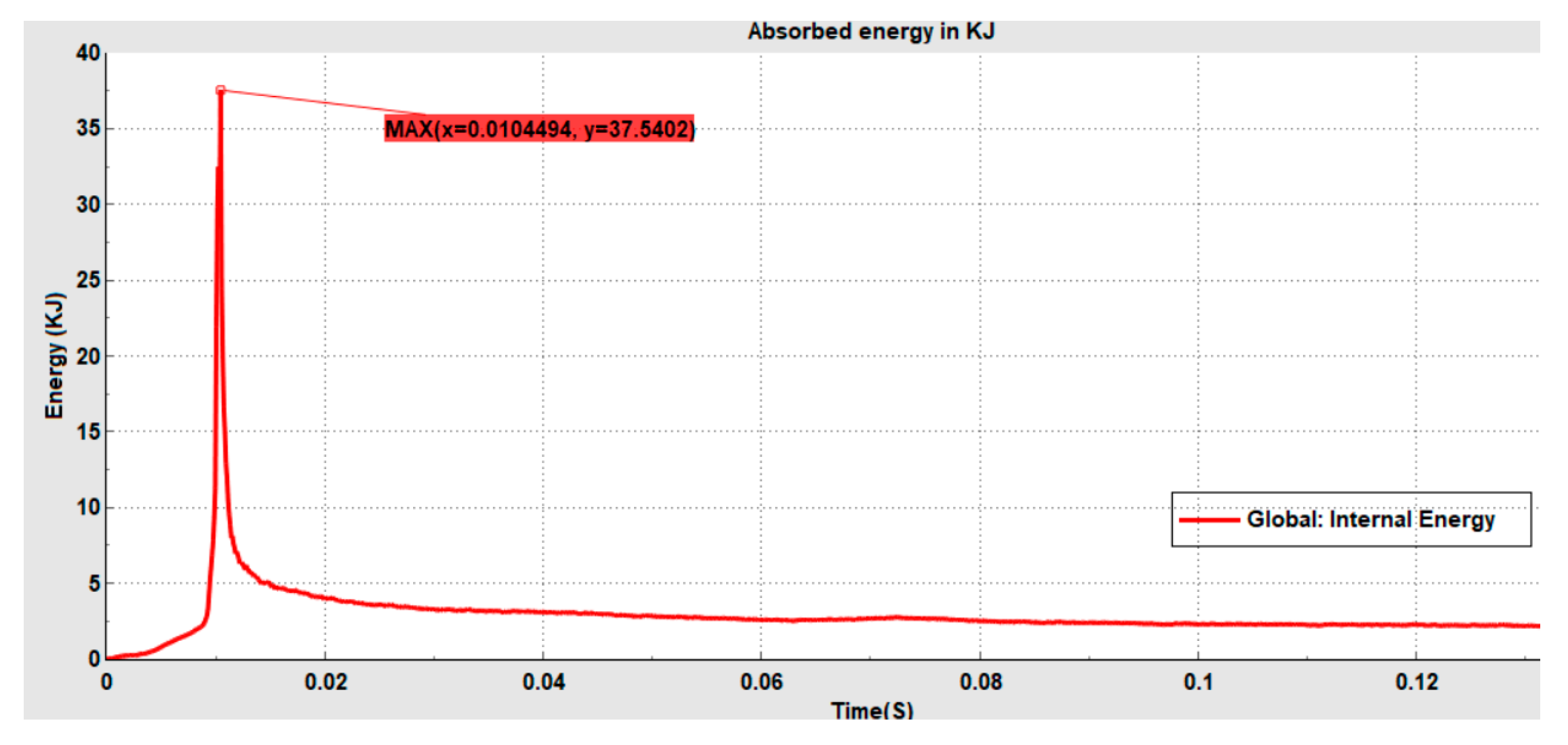
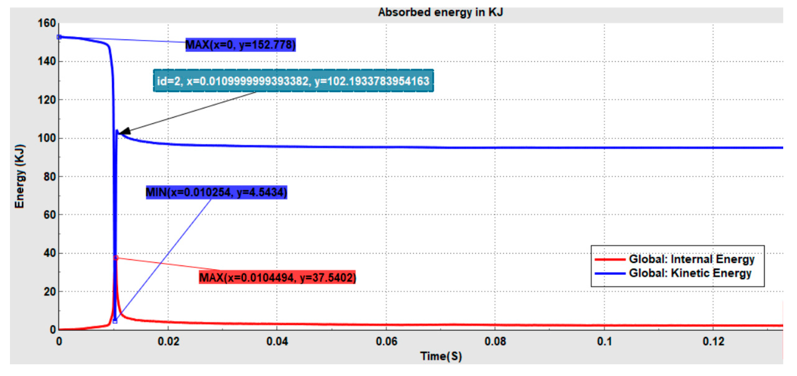
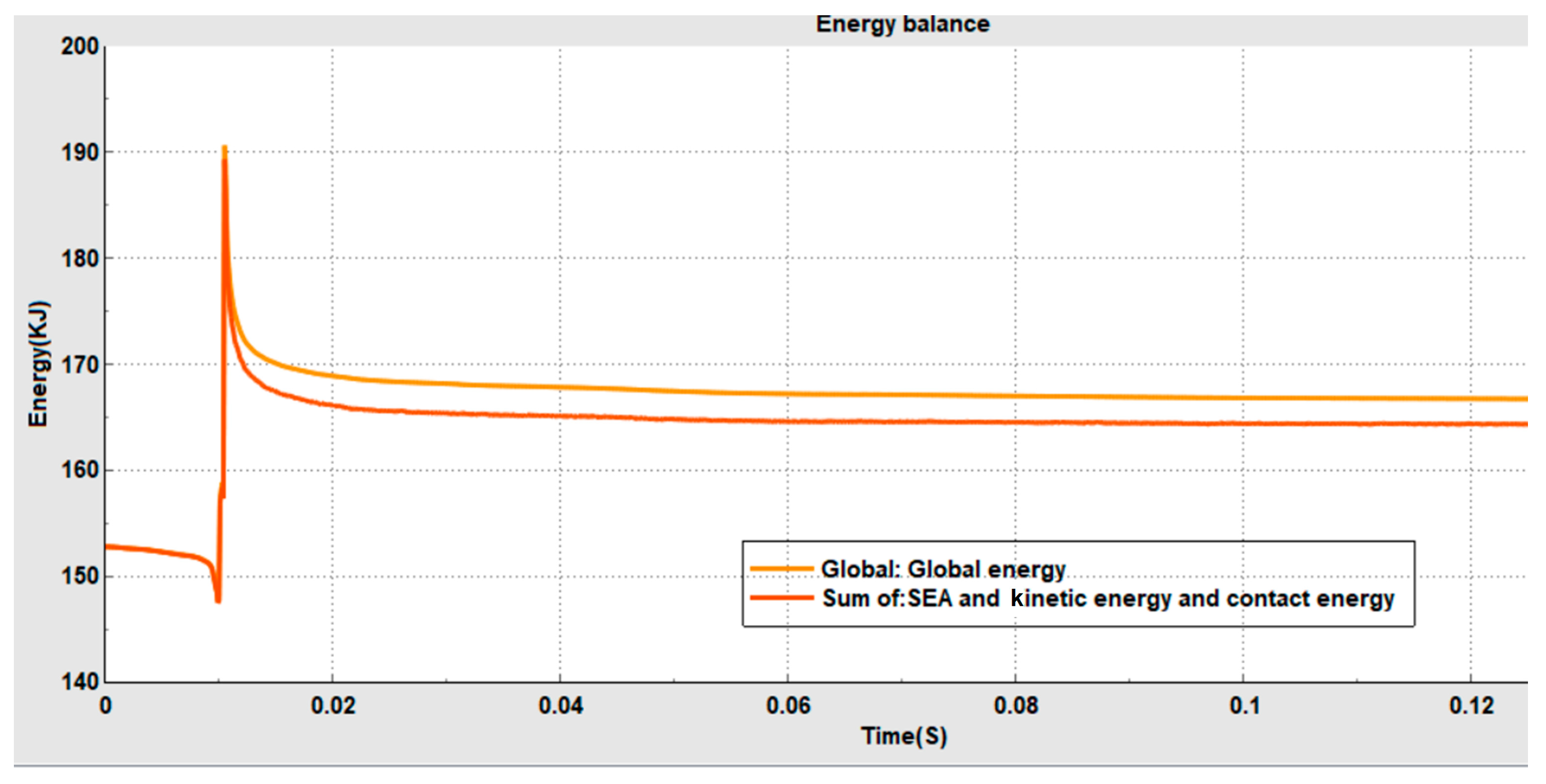
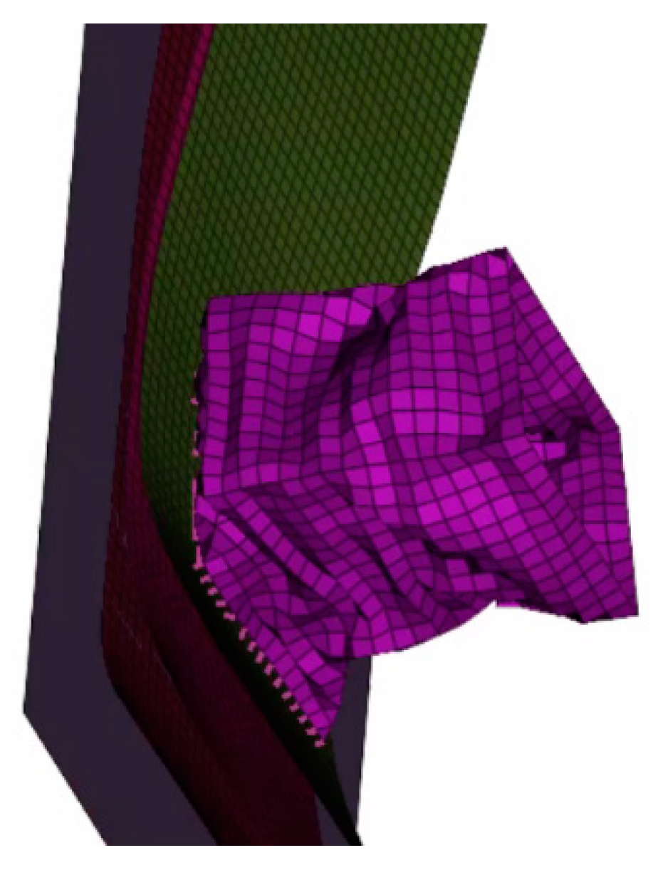
4.2. Load Case Application and Numerical Result

A rigid wall with 1100 kg moving with a velocity of 60 km/h has been deployed as an impactor to simulate the damage of the crash box in two cases of study with the same geometry and the same CFRP material. The following figure shows the ANSA representation of this load case (Figure 26 and Figure 27):

This paragraph focuses on the post-processing stage of the numerical model, simulated using the Chang failure as well as without introducing it into the simulation, which is aimed at comparing the structure’s behavior and the energy balance during the impact (Figure 28, Figure 29 and Figure 30).

The absorbed energy has demonstrated a brittle behavior that performs well with the mechanical characteristics of the CFRP materials. This is explained by a highly restricted range of plasticity as well as the absorbed energy’s being very small compared to the kinetic energy, which is a logical finding because brittle materials do not absorb this energy during impact due to the inability of crystal planes to slip with these materials, as shown in the following curves(Figure 31 and Figure 32):

The superposition of two curves confirms that the time of breaking up is 0.10 s; therefore, the pertinent question is, Where is the rest of this energy? The following curves describe how the contact energy + kinetic energy rotational energy + SEA equals the global energy of the crash test.

The gap between these curves is explained by the rotational behavior of the element as well as the hourglass energy (Figure 33 and Figure 34) [32].

One of the most reliable methodologies for verifying the numerical stability of the simulation is to use the added mass calculation [33,34]. The following figure illustrates the proposed methodology, with an added mass of 2.96 g:

Using the same input data as preprocessing without introducing the Chang criteria, the following figures show how the crash box will be damaged with large deformation and high internal energy, which explains the significant advantages that this technique affords (Figure 35, Figure 36, Figure 37 and Figure 38).

The results of the kinetic energy, the SEA, and the added mass obtained from the numerical simulation underscore the robustness of this study and bolster the hypotheses put forth in this paper, demonstrating the efficiency of the Chang failure criteria. By comparing the results with the Hashin criterion’s behavior [35], the authors confidently assert the conformity and reliability of their findings. However, within this confirmation lies a crucial and pressing question: Which criteria ultimately demonstrate superiority in simulating CFRP material crash damage: the Chang criteria or the Hashin criterion?

5. Conclusions

The main purpose of this paper was to carefully investigate and compare the performance of the Chang failure criteria with the simple FEM in optimizing the simulation of CFRP materials to become a more realistic factor in order to train engineers to simulate the vehicle components of CFRP materials.

It is essential to recognize the dominant trend in numerical simulations of fracture formation, which primarily concerns orthotropic materials. This requires starting with the creation of governing equations for the dynamics before taking Newmark’s method as the most adaptive for explicit dynamic calculation [36].

Through this research, the authors have been able to combine the LAW 25 for CRASURSV [37] composite shell element and the Chang failure criteria using a powerful preprocessor, including the Radioss Altair library known as ANSA CAE, and the numerical result was post-processed with META. The Chang failure criteria is considered one of the best for CFRP materials in crash calculations for several reasons [38,39,40]:

• Matrix damage modeling: Focuses on matrix damage mechanisms in composite materials, which is important because matrix failure can have a large influence on how CFRP materials generally perform when impacted.
• All-inclusive method: The Chang criteria consider many loading scenarios and failure modes, such as compressive and tensile stresses. This makes it possible to predict failure in different impact scenarios with greater accuracy.
• Material specificity: As the criteria are designed specifically for composite materials, they are more applicable than broader failure theories, which may not be able to explain the particular behavior of CFRP in crash scenarios.
• Predictive accuracy: Research has indicated that applying the Chang criteria can improve correlations between experimental data and findings, resulting in more reliable estimates of structural integrity and crash data.
• Progressive failure analysis is a crucial tool for understanding how damage develops in composite materials during collisions.
• The Chang criteria offer valuable information about the energy absorption and overall crashworthiness of a material.

While the Chang failure criteria represent a useful tool for predicting composite failure under simple loading conditions, especially in terms of tensile, compressive and shear failure, the method has some key limitations when applied to more complex situations. These limitations include its inability to model progressive damage, account for multiaxial stress states or incorporate environmental and fatigue effects. Therefore, when using these criteria, it is important to recognize these boundaries and consider complementary methods (such as progressive damage models or Finite Element Analysis) to more accurately predict composite failure in real-world applications.

The main query raised in our paper was as follows: Why do we continue to use the FEM without these criteria in industrial applications? Moreover, why do we not use aerodynamic conditions in crash engineering with the development of technical solutions to added mass problems using the methodologies described in [20,41]?

Regarding the perspective of this work, we aim in the near future to explore the Isogeometric Analysis (IGA) method to perform 3D calculations and demonstrate its capability to produce better results than the traditional Finite Element Method (FEM). Additionally, we will investigate the optimization methods already used in our teams to mitigate crash simulation in the object to minimize the computation time and simplify the model’s construction and management [42,43,44,45].

References

1. Wang, Y.; Mehler, B.; Reimer, B.; Lammers, V.; D’ambrosio, L.A.; Goughlin, J.F. The validity of driving simulation for assessing differences between in vehicle informational interfaces: A comparison with field testing. Ergonomics 2010, 53, 404–420. [Google Scholar] [CrossRef] [PubMed]
2. Kumar, S.; Bharj, R.S. Emerging composite material use in current electric vehicle: A review. Mater. Today Proc. 2018, 5, 27946–27954. [Google Scholar] [CrossRef]
3. Halimah, P.N.; Rahardian, S.; Budiman, B. Battery Cells for Electric Vehicles. Int. J. Sustain. Transp. Technol. 2019, 2, 54–57. [Google Scholar] [CrossRef]
4. El-Mekkaoui, J.; Elkhalfi, A.; Elakkad, A. Resolution of stokes equations with the Ca,b boundary condition using mixed finite element method. Trans. Math. 2013, 12, 586–597. [Google Scholar]
5. Lanzerath, H.; Nowack, N.; Mestres, E. Simulation Tool Including Failure for Structural Adhesives in Full-Car Crash Models; Technical Report; SAE: Pittsburgh, PA, USA, 2009. [Google Scholar]
6. van Ratingen, M.; Williams, A.; Lie, A.; Seeck, A.; Castaing, P.; Kolke, R.; Adriaenssens, G.; Miller, A. The European New Car Assessment Programme: A historical review. Chin. J. Traumatol. 2016, 19, 63–69. [Google Scholar] [CrossRef] [PubMed]
7. Ciampaglia, A.; Patruno, L.; Ciardiello, R. Design of a Lightweight Origami Composite Crash Box: Experimental and Numerical Study on the Absorbed Energy in Frontal Impacts. J. Compos. Sci. 2024, 8, 224. [Google Scholar] [CrossRef]
8. Hattori, G.; Rojas-Díaz, R.; Sukumar, A.S.; García-Sánchez, F. New anisotropic crack-tip enrichment functions for the extended finite element method. Comput. Mech. 2012, 50, 591–601. [Google Scholar] [CrossRef]
9. Barnes, G.; Coles, I.; Roberts, R.; Adams, D.O.; Garner, D.M. Crash Safety Assurance Strategies for Future Plastic and Composite Intensive Vehicles (PCIVS); Technical Report; U.S. Department of Transportation: Cambridge, MA, USA, 2010.
10. Abdullah, N.A.; Sani, M.S.; Salwani, M.S.; Husain, N.A. A review on crashworthiness studies of crash box structure. Thin-Walled Struct. 2020, 153, 106795. [Google Scholar] [CrossRef]
11. Liu, H.; Huang, J.; Zhang, W. Numerical algorithm based on extended barycentric Lagrange interpolant for two dimensional integro-differential equations. Appl. Math. Comput. 2021, 396, 125931. [Google Scholar] [CrossRef]
12. Chukwuemeke, W.I.; Chidozie, E. A review of the crashworthiness performance of energy absorbing composite structure within the context of materials, manufacturing and maintenance for sustainability. Compos. Struct. 2021, 257, 113081. [Google Scholar]
13. Xue, J.; Wang, W.X.; Zhang, J.Z.; Wu, S.J. Progressive failure analysis of the fiber metal laminates based on chopped carbon fiber strands. J. Reinf. Plast. Compos. 2015, 34, 364–376. [Google Scholar] [CrossRef]
14. Zhang, Z.; Niemi, E. A new failure criterion for the Gurson-Tvergaard dilational constitutive model. Int. J. Fract. 1994, 70, 321–334. [Google Scholar] [CrossRef]
15. Li, L.; Zhang, Y.; Cui, X.; Said, Z.; Sharma, S.; Liu, M.; Gao, T.; Zhou, Z.; Wang, X.; Li, C. Mechanical behavior and modeling of grinding force: A comparative analysis. J. Manuf. Process. 2023, 102, 921–954. [Google Scholar] [CrossRef]
16. Teodorescu-Draghicescu, H.; Vlase, S. Homogenization and averaging methods to predict elastic properties of pre-impregnated composite materials. Comput. Mater. Sci. 2011, 50, 1310–1314. [Google Scholar] [CrossRef]
17. Dag, S.; Arman, E.; Yildirim, B. Computation of thermal fracture parameters for orthotropic functionally graded materials using Jk–integral. Int. J. Solids Struct. 2010, 47, 3480–3488. [Google Scholar] [CrossRef]
18. Bui, T.Q. Extended isogeometric dynamic and static fracture analysis for cracks in piezoelectric materials using NURBS. Comput. Methods Appl. Mech. Eng. 2015, 295, 470–509. [Google Scholar] [CrossRef]
19. Xu, X.; Ou, J.P. Force identification of dynamic systems using virtual work principle. J. Sound Vib. 2015, 337, 71–94. [Google Scholar] [CrossRef]
20. Zhiqing, C.; Reagan, P.H.; Sieveka, S. Experiences in reverse-engineering of a finite element automobile crash model. Finite Elem. Anal. Des. 2001, 37, 843–860. [Google Scholar]
21. Yang, H.; Shao, L.; Ou, J.; Zhou, Z. A Novel Smart CFRP Cable Based on Optical Electrical Co-Sensing for Full-Process Prestress Monitoring of Structures. Sensors 2023, 23, 5261. [Google Scholar] [CrossRef]
22. Essam, M.; Almitani, K. Detecting Damage in Carbon Fibre Composites using Numerical Analysis and Vibration Measurements. Lat. Am. J. Solids Structures 2021, 18, e362. [Google Scholar]
23. Bai, B.; Ci, H.; Lei, H.; Cui, Y. A local integral-generalized finite difference method with mesh-meshless duality and its application. Eng. Anal. Bound. Elem. 2022, 139, 14–39. [Google Scholar] [CrossRef]
24. McLachlan, R.I. Spatial Discretization of Partial Differential Equations with Integrals. IMA J. Numer. Anal. 2003, 23, 645–664. [Google Scholar] [CrossRef]
25. Moes, N.; Belytschko, T. X-FEM, de nouvelles frontières pour les éléments finis. Eur. J. Comput. Mech. 2012, 11, 305–318. [Google Scholar] [CrossRef]
26. Meo, M.; Morris, A.J.; Vignjevic, R.; Marengo, G. Numerical simulations of low-velocity impact on an aircraft sandwich panel. Compos. Struct. 2003, 62, 353–360. [Google Scholar]
27. Chang, F.K.; Chang, K.Y. A Progressive Damage Model for Laminated Composites Containing Stress Concentrations. J. Compos. Mater. 1987, 21, 834–855. [Google Scholar] [CrossRef]
28. Thanh, N.; Josef, K. Rotation free isogeometric thin shell analysis using PHT-splines. Comput. Methods Appl. Mech. Eng. 2011, 200, 3410–3424. [Google Scholar] [CrossRef]
29. Carello, M.; Airale, A.; Ferraris, A.; Messana, A.; Sisca, L. Static Design and Finite Element Analysis of Innovative CFRP Transverse Leaf Spring. Appl. Compos. Mater. 2017, 27, 1493–1508. [Google Scholar] [CrossRef]
30. Qu, C.J.; Xu, P.; Yao, S.G.; Yang, C.X.; Jin, X.H. Crash Stability Analysis and Multi-Objective Optimization of Oriented Energy-Absorbing Structure for Locomotive. Int. J. Struct. Stab. Dyn. 2023, 23, 2350175. [Google Scholar] [CrossRef]
31. Shao, J.; Liu, N.; Zheng, Z. Numerical comparison between Hashin and Chang-Chang failure criteria in terms of inter-laminar damage behavior of laminated composite. Mater. Res. Express 2021, 8, 2053–2159. [Google Scholar] [CrossRef]
32. Isaac, M.D. Constitutive behavior and failure criteria for composites under static and dynamic loading. Meccanica 2015, 50, 429–442. [Google Scholar]
33. Rizal, K.; Syaifudin, A. Evaluation of Crash Energy Management of the First-Developed High-Speed Train in Indonesia. J. Eng. Technol. Sci. 2023, 55, 235–246. [Google Scholar] [CrossRef]
34. Nguyen, V.P.; Bordas, S.; Rabczuk, T. Isogeometric analysis: An overview and computer implementation aspects. Math. Comput. Simul. 2015, 117, 89–116. [Google Scholar] [CrossRef]
35. Sundeep, M.; Harpreet, A.; Medha, V. Performance and Design of Steel Structures Reinforced with FRP Composites: A state-of-the-art review. Eng. Fail. Anal. 2023, 138, 106371. [Google Scholar]
36. Chang, S.Y. Studies of Newmark method for solving nonlinear systems: (I) basic analysis. J. Chin. Inst. Engineers 2004, 27, 651–662. [Google Scholar] [CrossRef]
37. Mamalis, A.G.; Manolakos, D.E.; Ioannidis, M.B.; Papapostolou, D.P. On the response of thin-walled cfrp composite tubular components subjected to static and dynamic axial compressive loading: Experimental. Compos. Struct. 2005, 69, 407–420. [Google Scholar] [CrossRef]
38. Barros, F.; Silva, R. Extended isogeometric analysis: A two-scale coupling FEM/IGA for 2D elastic fracture problems. Comput. Mech. 2023, 73, 639–665. [Google Scholar]
39. Johnson, A.F. Modelling fabric reinforced composites under impact loads. Compos. Part A Appl. Sci. Manuf. 2001, 32, 1197–1206. [Google Scholar] [CrossRef]
40. Pao, Y.H.; Wang, L.S.; Chen, K.C. Principle of Virtual Power for thermomechanics of fluids and solids with dissipation. Int. J. Eng. Sci. 2011, 49, 1502–1516. [Google Scholar] [CrossRef]
41. Koubaiti, O.; El-Mekkaoui, J.; Elkhalfi, A. Complete study for solving Navier-Lamé equation with new boundary condition using mini element method. Int. J. Mechanics 2018, 12, 46–56. [Google Scholar]
42. Hughes, T.; Bazilevs, Y. Isogeometric analysis: CAD, finite elements, NURBS, exact geometry and mesh refinement. Comput. Methods Appl. Mech. Eng. 2005, 194, 4135–4195. [Google Scholar] [CrossRef]
43. Berrada-Gouzi, M.; El Khalfi, A.; Vlase, S.; Scutaru, M.L. X-IGA Used for Orthotropic Material Crack Growth. Materials 2024, 17, 3830. [Google Scholar] [CrossRef] [PubMed]
44. Montassir, S.; Moustabchir, H.; Elkhalfi, A.; Scutaru, M.L.; Vlase, S. Fracture modelling of a cracked pressurized cylindrical structure by using extended iso-geometric analysis (X-IGA). Mathematics 2021, 9, 2990. [Google Scholar] [CrossRef]
45. El Fakkoussi, S.; Moustabchir, H.; Elkhalfi, A.; Pruncu, C.I. Application of the extended isogeometric analysis (X-IGA) to evaluate a pipeline structure containing an external crack. J. Eng. 2018, 2018, 4125765. [Google Scholar] [CrossRef]
Figure 1. Translation behavior mode 1-2.
Mathematics 12 03673 g001
Figure 2. Translation behavior mode 3-4.
Mathematics 12 03673 g002
Figure 3. Translation behavior mode 5-6.
Mathematics 12 03673 g003
Figure 4. Translation behavior mode 7-8.
Mathematics 12 03673 g004
Figure 5. Translation behavior mode 9.
Mathematics 12 03673 g005
Figure 6. Translation behavior mode 10.
Mathematics 12 03673 g006
Figure 7. Translation behavior mode 11.
Mathematics 12 03673 g007
Figure 8. Translation behavior mode 12.
Mathematics 12 03673 g008
Figure 9. Rotational behavior mode 1.
Mathematics 12 03673 g009
Figure 10. Rotational behavior mode 2.
Mathematics 12 03673 g010
Figure 11. Rotational behavior mode 3.
Mathematics 12 03673 g011
Figure 12. Rotational behavior mode 4.
Mathematics 12 03673 g012
Figure 13. Rotational behavior mode 5-6.
Mathematics 12 03673 g013
Figure 14. Rotational behavior mode 7-8.
Mathematics 12 03673 g014
Figure 15. Rotational behavior mode 9-10.
Mathematics 12 03673 g015
Figure 16. Rotational behavior mode 11-12.
Mathematics 12 03673 g016
Figure 17. Numerical procedure flow chart.
Mathematics 12 03673 g017
Figure 18. Typical structure of carbon fiber reinforced polymer (CFRP).
Mathematics 12 03673 g018
Figure 19. Carbon fiber compared with human hair.
Mathematics 12 03673 g019
Figure 20. Global coordinate system of the laminate.
Mathematics 12 03673 g020
Figure 21. CFRP material tensile stress–strain behavior.
Mathematics 12 03673 g021
Figure 22. Normal behavior of load versus displacement for CFRP impact.
Mathematics 12 03673 g022
Figure 23. Crash box in CFRP material dimensions.
Mathematics 12 03673 g023
Figure 24. Crash box + transversal bar representation.
Mathematics 12 03673 g024
Figure 25. T7 contact between crash box (slaves in red color) and transversal bar (master in blue color).
Mathematics 12 03673 g025
Figure 26. Moving rigid wall impact.
Mathematics 12 03673 g026
Figure 27. Fixation of the crash box.
Mathematics 12 03673 g027
Figure 28. Damage at t = 0 (Chang failure).
Mathematics 12 03673 g028
Figure 29. Damage at t = 0.4 ms (Chang failure).
Mathematics 12 03673 g029
Figure 30. Damage at t = 10 ms (Chang failure).
Mathematics 12 03673 g030
Figure 31. SEA energy during crash.
Mathematics 12 03673 g031
Figure 32. SEA energy and kinetic energy.
Mathematics 12 03673 g032
Figure 33. Impact of the energy balance.
Mathematics 12 03673 g033
Figure 34. Added mass of crash simulation.
Mathematics 12 03673 g034
Figure 35. Damage at t = 0 without Chang criteria.
Mathematics 12 03673 g035
Figure 36. Damage at t = 4 ms without Chang criteria.
Mathematics 12 03673 g036
Figure 37. Damage at t = 8 ms without Chang criteria.
Mathematics 12 03673 g037
Figure 38. Damage at t = 12 ms without Chang criteria.
Mathematics 12 03673 g038