Article

Aperiodic Optimal Chronotherapy in Simple Compartment Tumour Growth Models Under Circadian Drug Toxicity Conditions

by
Byron D. E. Tzamarias
1,
Annabelle Ballesta
2 and
Nigel John Burroughs
3,*
1
MathSys CDT, Mathematics Institute, University of Warwick, Coventry CV4 7AL, UK
2
Inserm U900, Cancer Systems Pharmacology Team, Institut Curie, MINES ParisTech, CBIO, PSL Research University, 35 Rue Dailly, 92210 Saint-Cloud, France
3
SBIDER, Mathematics Institute, University of Warwick, Coventry CV4 7AL, UK
*
Author to whom correspondence should be addressed.
Mathematics 2024, 12(22), 3516; https://doi.org/10.3390/math12223516
Submission received: 11 October 2024 / Revised: 2 November 2024 / Accepted: 6 November 2024 / Published: 11 November 2024
(This article belongs to the Section E3: Mathematical Biology)

Abstract

:
Cancer cells typically divide with weaker synchronisation with the circadian clock than normal cells, with the degree of decoupling increasing with tumour maturity. Chronotherapy exploits this loss of synchronisation, using drugs with circadian-clock-dependent activity and timed infusion to balance the competing demands of reducing toxicity toward normal cells that display physiological circadian rhythms and of efficacy against the tumour. We analysed optimal chronotherapy for one-compartment nonlinear tumour growth models that were no longer synchronised with the circadian clock, minimising a cost function with a periodically driven running cost accounting for the circadian drug tolerability of normal cells. Using Pontryagin’s Minimum Principle (PMP), we show, for drugs that either increase the cell death rate or kill dividing cells, that optimal solutions are aperiodic bang–bang solutions with two switches per day, with the duration of the daily drug administration increasing as treatment progresses; for large tumours, optimal therapy can in fact switch mid treatment from aperiodic to continuous treatment. We illustrate this with tumours grown under logistic and Gompertz dynamics conditions; for logistic growth, we categorise the different types of solutions. Singular solutions can be applicable for some nonlinear tumour growth models if the per capita growth rate is convex. Direct comparison of the optimal aperiodic solution with the optimal periodic solution shows the former presents reduced toxicity whilst retaining similar efficacy against the tumour. We only found periodic solutions with a daily period in one-compartment exponential growth models, whilst models incorporating nonlinear growth had generic aperiodic solutions, and linear multi-compartments appeared to have long-period (weeks) periodic solutions. Our results suggest that chronotherapy-based optimal solutions under a harmonic running cost are not typically periodic infusion schedules with a 24 h period.

1. Introduction

In mammals, most physiological processes exhibit 24 h rhythmicity, the so-called circadian rhythms [1]. This is the result of a hierarchical circadian timing system governed by a masterclock, the suprachiasmatic nucleus (SCN) located in the hypothalamus, that displays spontaneous circadian oscillations entrained to a period of exactly 24 h by external cues such as light [2]. The SCN sends synchronization signals to the circadian clock circuit present in each cell of the body; this circuit is a gene–protein circuit composed of approximately 20 elements coupled through feedback loops [3,4]. In mice, 43% of genes display a circadian rhythm somewhere in the body [5]. Cell division has an input from the circadian clock, namely, 1:1 phase locking occurring in vitro [4,6].
The circadian timing system is often perturbed in pathological conditions, and two crucial observations relevant to cancer and its treatment have been made in the last decade. Firstly, disruption of the body’s circadian rhythm, such as that observed in shift workers, is a risk factor in cancer and many other conditions [7,8]. Secondly, the efficacy and side effects of many treatments are affected by the circadian timing of the intervention [9]. In particular, the circadian rhythms of an organism affect the absorption, distribution, metabolism, elimination, and transportation of anticancer drugs, possibly leading to timing-dependent efficacy of treatments [1]. Further, drugs that target cells in specific phases of the cell cycle, e.g., 5-fluorouracil (5-FU), may also have an efficacy that is dependent on the time of day [10,11]. Cancer cells often have a degraded circadian clock or a reduced degree of coupling with the body’s circadian rhythm, imparting a perturbed, shifted, or even arrhythmic intracellular circadian rhythm [12]. The varying efficacy of chemotherapy drugs with respect to the phase of the clock can thus result in a difference in toxicity between cancer cells and normal cells depending on the time day. This has lead to the emergence of chronotherapy.
Chrono-modulated chemotherapy, or chronotherapy, consists of administrating drugs at specific phases of a patient’s circadian rhythm to maximise the drugs’ efficacy whilst minimising their toxicity toward normal cells. Multiple clinical trials have demonstrated reduced toxicity and improved efficacy of chronotherapy across a range of chemotherapy drugs [13,14,15,16]. A disregard of the importance of chronomodulation is well illustrated by the case of Oxaliplatin (OXP): the initial Phase I trials were abandoned, and only when OXP was re-examined with chronomodulated delivery did its value become apparent. It is now a key chemotherapy drug [16]. The time of day when radiotherapy is administered was shown to affect treatment tolerability in a retrospective analysis of patient data [17].
A central question in cancer therapy is how to balance the competing objectives of maximising the efficacy of a drug against the tumour and minimising toxicity toward healthy cells (and to the patient generally). A number of studies have investigated specific drug-timing protocols through simulations, using detailed models of the circadian clock and tumour cell cycle heterogenity [18,19,20,21]. These studies demonstrated distinct efficacy gains with chronomodulation. In [22], a cellular automaton model of the cell cycle was employed to study the dependence of drug toxicity on the circadian timing of two anti-cancer agents (OXP and 5-FU). For a non-malignant cell population entrained by the circadian clock (with an average cell cycle length of 22 h), these drugs should be administered at specific times of day to minimise cytotoxicity and in antiphase; OXP and 5-FU, in fact, kill cells at different phases of the cell cycle.
Optimal Control Theory (OCT) is a methodology used to determine the optimal solutions to a problem formulated as a minimisation (or maximisation) of a specified objective function. It has been widely applied in the context of optimising drug delivery schedules in cancer chemotherapy treatments, with multiple reviews [23,24,25,26] and books having been dedicated to the subject [27,28,29]. Typically, the competing objectives of maximising efficacy against the tumour whilst minimising toxicity toward the patient are combined as a weighted sum into a single cost function that is then minimised over the degrees of freedom, including the drug dose and schedule [29], although a few recent studies use multi-objective methods [30]. Models can also include the drug’s pharmacokinetics/pharmakodynamics (PK/PD) [31,32,33,34,35].
Despite the fact that OCT has been widely applied in the context of cancer therapy, there are few studies focusing on optimising chronotherapy treatments. In a proof-of-concept study using the human colon cancer cell line Caco-2 [32], the optimal timing of irinotecan was shown to be around CT5 (CT = circadian time, with CT0 being defined as the start of cell synchronization via serum shock), starting 1.5 h before the nadir of the drug-activating enzyme carboxylesterase 2 in healthy cells. This study developed a detailed PK/PD model parametrised from data and used a cost function based on DNA damage. In an earlier work, ref. [33] examined chronotherapy treatments for OXP for mice with osteosarcoma. The effect of the circadian clock on the drug’s toxicity toward healthy tissue (the mature jejunal enterocyte population) and antitumour efficacy were taken into account. Optimal containment solutions within a prescribed 2–5-infusion cycle had variable drug-dosing levels, a schedule that kept the tumor cell population at a low level while preserving the jejunal cell population. Both works used restricted drug delivery schedules, so drawing general chronotherapy conclusions is not possible.
In this work, we applied OCT to simple tumour growth models to determine the general principles of an optimal chronotherapy drug treatment, with the simple models used allowing analytical results to be obtained. We assumed treatment comprises a single chemotherapy drug administered by an infusion device that controls the concentration of the drug throughout the day. We assumed that the drug’s toxicity toward healthy cells is circadian-rhythm-dependent, whilst the cancer cells are totally decoupled from the circadian clock, for instance, through the loss of either their cellular circadian clock or their synchronisation with external signals. Thus, by modulating the concentration of the drug throughout the day, its toxicity toward normal cells can be reduced whilst its efficacy against cancer cells can be retained [15]. The optimal drug administration schedule was determined by minimising a cost function comprising a terminal cost proportional to the tumor size and a periodically driven running cost that models the toxicity of the drug toward healthy cells. The cost functional was minimised using Pontryagin’s Minimum Principle (PMP) [36].
This paper is organised as follows. In Section 2, the cost function is introduced. In Section 3, the periodicity and singularity of the optimal solutions for two types of drug action are examined, specifically cytotoxic drugs and drugs that kill cells during cell division. We prove that solutions are of the bang–bang type and aperiodic, with two switches per day, for generic growth models with a concave per capita growth rate; i.e., daily drug infusion occurs for varying durations. In Section 4, the logistic tumor growth model is examined in detail; solutions that satisfy PMP are categorised as trajectories in the N w plane, where tumour size is denoted by N and w is the product of the tumor size N and the costate p. There can be multiple trajectories for some initial conditions w 0 ; specifically, trajectories can be extended, giving another solution with a larger time horizon satisfying the transversality condition at a later time. In Section “The Cost and Treatment Time of Optimal Solutions”, the dependence of the cost and the time horizon on w 0 is studied. For the optimal solution, i.e., the trajectory with the lowest cost, the drug is typically administered during an interval of each day, with the length of this interval increasing as treatment progresses. In Section 5, the cost function is minimised for the Gompertz growth model. We utilise a numerical method that exploits the bang–bang structure of the optimal solutions, generating solutions with high accuracy over large time scales and hundreds of switching events, being more accurate than direct optimisation numerical methods, which can, in fact, fail. Similar results to the logistic model were found, with both models exhibiting the same categories of optimal solutions in the N w plane. In both cases, the optimal solutions with the smallest cost are therapies wherein a drug is administered during a fraction of each day, with the daily drug administration interval increasing as the treatment progresses. In Section 6, we extend our analysis to multi-compartment models; for linear growth, the optimal solutions are bang–bang. For a two-compartment cell cycle model, we find solutions that satisfy PMP numerically. These are aperiodic and cheaper than the optimal solution constrained to entail periodic daily drug administration.
In Section 7, we demonstrate the advantages of the optimal aperiodic solutions over the optimal solutions in which the drug is administered continuously at the maximum tolerated dose and optimal periodic solutions. The benefits of the aperiodic solutions increase with the size of the tumour and its sensitivity to the drug.

2. The Cost Function

The objective of treatment is to minimise the number of cancer cells whilst minimising toxicity toward normal cells, constituting two conflicting objectives. To balance these factors, an objective function weighting these requirements is used. We use the following cost functional:
J [ N , u ] = r N ( T ) + d 0 T h ( t ) u ( t ) d t ,
where time is measured in days, N ( t ) is the number of cancer cells at time t, and u ( t ) is the drug concentration, the control. Drug concentration is limited by the maximum tolerated dose (MTD), which is the maximum concentration that can be administered. We scale drug concentrations to the MTD so that u ( t ) [ 0 , 1 ] . Toxicity toward normal cells is dependent on the phase of the circadian clock; this is captured by the positive periodic function h ( t ) , with a single minimum and maximum per day. We will use h ( t ) = 1 d ( 1 α cos ( 2 π t ) ) for illustration, where | α | 1 parametrises the degree of influence of the clock. We assume that α ( 0 , 1 ) and that treatment starts at noon ( t = 0 ), when healthy cells have a higher tolerance to the drug. T is the time horizon, and r is a positive constant weighting the terminal tumor size N ( T ) relative to the running cost. We introduce d, the death rate of tumour cells, into the definition of h ( t ) for convenience later on, with the cost function being independent of d. The parameter r determines the relative weighting of the conflicting objectives to minimise the final tumour size and minimise patient toxicity. We want to find optimal schedules of the drug, u ( t ) , that minimise this cost functional. Admissible controls are piecewise continuous functions: u ( t ) C ^ [ 0 , T ] [37].

3. Existence of Aperiodic Solutions in Chronotherapy

We examine optimal solutions for two types of drugs: firstly, cytotoxic drugs, for which the drug concentration increases the death rate of tumour cells, and, secondly, cell cycle drugs, for which the tumour’s growth rate is decreased by the drug, modelling the drugs that act only during cell division. These differ in terms of the manner in which the drug affects tumour dynamics, but both exhibit a toxicity toward normal cells that is circadian-rhythm-dependent. Below, we prove two theorems for fixed time horizon optimisation problems. We use Pontryagin’s Minimum principle [36], which gives the necessary conditions for the optimal solutions. Since we have admissible controls, for instance, a constant u is admissible, an optimal solution exists. If the solution to PMP is unique, it is then considered the optimal solution, whilst if PMP gives multiple solutions, the one with the minimum cost is the desired optimal solution. We determine all solution branches to PMP over variable time horizons, allowing us to determine the optimal solution for a specified time horizon.

3.1. Cytotoxic Drugs

Consider the tumour growth dynamic
d N d t = g ( N ) N d u N , N ( 0 ) = N 0
with a net tumour cell growth rate g ( N ) in the absence of the drug satisfying d g d N < 0 , which captures competition for resources. We assume a capacity of N * in the absence of a drug satisfying g ( N * ) = 0 ; thus the physical size range of the tumour is N ( t ) [ 0 ,   N * ) . The second term is drug-induced cell death; the drug concentration is rescaled so that u ( t ) [ 0 ,   1 ] such that the upper bound, 1, is the MTD and d > g ( 0 ) so that at MTD the tumour can be eliminated. For the special case where g ( N ) is constant (exponential growth), the optimal solution is of the bang–bang type, and u is periodic, with a period of 1 day (see Appendix A). Nonlinear growth, however, removes this periodicity, as we show below.
Theorem 1. 
(Drugs targetting death/cytotoxic drugs).
The optimal solutions that minimise the cost function (1) for a fixed horizon time  T 2  with tumour growth dynamics (2) are any of the following (subject to parameters and initial tumour size):
  • Constant drug administration, specifically with no treatment ( u = 0 ) or MTD ( u = 1 );
  • Bang–bang aperiodic solutions, with two switches per day and a non-decreasing daily drug administration interval;
  • An order 1 singular arc with a duration  < 12  h that satisfies
    d g ( N ) d N N = d log h ( t ) d t .
    A necessary condition for the singular arc to exist is  N d 2 g d N 2 ( N ) d g ( N ) d N .
Solutions can be concatenated.
  • Comment: Bang–bang solutions can be constructed, and thus one can determine if they intersect the singular arc, a segment of a circle in the ( N , w ) plane, with w ( t ) = h ( t ) , N ( t ) , satisfying the above arc condition. The singular arc only needs to be considered if there is an intersection.
  • Comment: The singular arc has a log tumour size change of less than d / 2 , so it cannot contribute to substantial tumour decay.
Proof. 
We use PMP to derive the optimal solutions and examine the singular arc solutions using the Legendre–Clebsch (LC) conditions [38]. The generalized LC conditions are necessary conditions of optimality for singular solutions; singular solutions have an order of j 0 , the smallest integer such that u d j 0 d t j 0 H ˜ u 0 . The order j 0 is even, and an optimal solution minimises the objective function only if the quantity ( 1 ) p u d j 0 d t j 0 H u > 0 , with p = j 0 2 ; conversely, it is a maximiser if it is negative.
Since the objective function’s running cost has explicit time dependence in our case, we extend the system by introducing the additional state variable y, with d y d t = 1 , y ( 0 ) = 0 and an associated costate q. PMP equations are, in fact, identical to the autonomous PMP ignoring time dependence, except the Hamiltonian is not constant in this case (see Appendix B). In brief, the Hamiltonian of the extended system is H ˜ = H + q , where H is the Hamiltonian of the original system, and therefore H ˜ u = H u . Thus, the LC conditions can also be applied to the original Hamiltonian H. (see Appendix B).
The Hamiltonian is given by
H N , p , u = g N d u N p + d h u ,
with p being the costate, the dynamics of which are given by
d p d t = d g d N N N + g ( N ) d u p ,   and   p ( T ) = r ( transversality   condition ) .
Since the Hamiltonian is linear in u, there is a switching function given by
Φ N , w , t = H u = d ( w h ) ,
with w = N p . By combining the adjoint Equation with the state Equation, we obtain
d w d t = w N d g d N .
The transversality condition then becomes w ( T ) = r N ( T ) > 0 . Trajectories can be visualised on the ( N , w ) plane, as shown in Figure 1. Since w = 0 is a w-nullcline and the termination line is in the positive quadrant, the trajectories have w > 0 for all oftime. w thus monotonically increases given that d g d N < 0 .
Since the objective is to minimise, the Hamiltonian is minimal at each time point giving the optimal drug concentration conditions:
  • u = 0 when Φ > 0 ; i.e., w ( t ) < h ( t ) .
  • u = 1 when Φ < 0 ; i.e., w ( t ) > h ( t ) .
  • A singular arc if Φ = 0 holds for an extended period; i.e., w ( t ) = h ( t ) .
Hence, there are three zones: for w > max ( h ) , we have u = 1 , and for w < min ( h ) , u = 0 , whilst when min ( h ) < w < max ( h ) , switching occurs (Figure 1).
The optimal solution thus satisfies a two-point boundary value problem, dynamics (2) and (3), with control being a function of w = p N , and an initial condition on N, terminal on p. This is typically solved using a shooting method [39]. By using a phase plane, we can classify all the trajectories, defining the family of solutions for the shooting method, thereby enabling the determination of the optimal solution (i.e., the lowest cost).
First, we consider the existence of singular arcs. We have the condition that H u = 0 , and all its time derivatives are zero for the duration of the singular arc, i.e.,
d H u d t = d N d g d N w + d h d t = 0 , d 2 H u d t 2 = d d N d t d g d N w + N w d 2 g d N 2 + N d g d N d w d t + d 2 h d t 2 = 0 .
The singular arc is thus first order since u d 2 H u d t 2 0 , and from the generalised Legendre–Clebsch condition [38], the arc is a minimum if u d 2 H u d t 2 0 . This gives the condition
d 2 w d g d N + N d 2 g d N 2 0 ,
as stated.
The singular arc in the ( N , w ) plane is thus given implicitly by
w ( t ) = h ( t ) , N ( t ) d g d N h ( t ) + d h d t = 0 .
This is a circle in the ( N , w ) plane, crossing N = 0 when d h d t = 0 . The projection on N gives the solution as stated. Clearly, any physical singular arc must have a tumour size of 0 < N < N * . The drug concentration on the arc is given by
u ( t ) = 1 d g ( N ) + d 2 h d t 2 1 h d h d t 2 N 2 h d 2 g d N 2 d h d t .
The location of the singular arc on the curve (5) can then be determined by imposing the condition that u ( t ) lies in [ 0 , 1 ] .
The solutions are otherwise bang–bang. There are two special cases with trajectories in zone 1, with u = 0 , and zone 3, with u = 1 . To address the periodicity of the bang–bang solutions that transit through the switching zone, i.e., zone 2, assume that there is a periodic solution u ( t ) , with a period of τ . To remain in the switching zone, there must be two switches a day. We define the switching times: t k = t 1 + k τ and t k = t 1 + k τ ; when w ( t k ) = h ( t k ) , w ( t k ) = h ( t k ) , with switches occurring from u = 1 to u = 0 and vice versa. However, w increases, and so we have h ( t k ) > h ( t k 1 ) , h ( t k ) > h ( t k 1 ) . But based on the form of h, the interval of being drug-free, t k t k , strictly decreases, constituting a contradiction since u must be periodic. Thus, there are no periodic solutions for T > 2 . We choose a horizon longer than 2 days to exclude special cases.
Correspondingly, if we assume the solution has a sequence of daily periodic switches, then we can show that g N = 0 . Between any two switching time points t k , t k + 1 , from u = 0 to u = 1 , we have
Φ ( t k + 1 ) Φ ( t k ) = d t k t k + 1 d w d t d t = 0
which follows since h ( t ) is periodic. Since w > 0 monotonically increases, this is only consistent if g N = 0 (4). □

3.2. Drugs Targeting Growth

Here, we consider drugs that kill during cell division. Consider the tumour growth dynamic
d N / d t = ( 1 d u ) g ( N ) N d 0 N
with, as above, d g d N < 0 and a capacity N * satisfying g ( N * ) d 0 = 0 . The drug concentration is rescaled so that u ( t ) [ 0 , 1 ] , where u = 1 is the MTD. Drug efficacy is determined by d, d 2 , where d = 2 would correspond to complete drug efficacy, with the drug killing all proliferating cells. Cytostatic drugs that slow or stop cells entering cell division are also included but have d 1 , although recent work suggests that cells prevented from entering cell cycle can die of osmotic stress [40], suggesting d may also be greater than 1. Here, d 0 is the natural death rate of tumour cells satisfying g ( 0 ) > d 0 ; if d 0 = 0 , then the application of the drug is a reparmetrisation of the growth trajectory; the optimal solutions are then periodic with a period of 1 day. This periodicity is lost when d 0 > 0 , as proven below.
Theorem 2. 
Drugs targeting proliferation (cell cycle drugs).
For d 0 > 0 and nonlinear growth d g d N 0 , the optimal solutions with a horizon of T 2 that minimise the cost (1) are any of the following (subject to parameters and initial tumour size):
  • Constant drug administration, specifically with no treatment ( u = 0 ) or MTD ( u = 1 );
  • Bang–bang aperiodic solutions, with two switches per day and a non-decreasing daily drug administration interval;
  • An order 1 singular arc with a duration of < 12 h that satisfies
    d 0 N d log g d N = d log h d t
    A necessary condition for the singular arc to exist is that N log ( d g d N ) monotonically decreases on the arc, which requires that d 2 g d N 2 > 0 .
Solutions can be concatenated.
  • Comment: The singular arc has a log tumour size range less than ( g ( 0 ) + d 0 ) / 2 and thus cannot contribute to substantial tumour decay.
Proof. 
Using Pontryagin’s Minimum Principle for non-autonomous systems (Appendix B), we can obtain the Hamiltonian H N , p , t = 1 u d g ( N ) N d 0 N p + d h u , where p is the costate. The switching function is
Φ N , w , t = d ( w h ) ,
with w = g ( N ) N p . Optimal solutions can be obtained under the following conditions:
  • u = 0 when Φ > 0 ; i.e., w ( t ) < h ( t ) .
  • u = 1 when Φ < 0 ; i.e., w ( t ) > h ( t ) .
  • A singular arc if Φ = 0 holds for an extended period; i.e., w ( t ) = h ( t ) .
The costate dynamics are given by
d p d t = 1 d u g ( N ) + d g ( N ) d N N p + d 0 p ,   with   p ( T ) = r .
As before, it is convenient to consider trajectories in the ( N , w ) plane. The variable w has the following dynamics:
d w d t = d 0 N w g ( N ) d g ( N ) d N = d 0 N w d d N log g ( N )
Since d w d t = 0 on w = 0 , we know that w > 0 for all of time since the termination condition gives w ( T ) = r g ( N ( T ) ) N ( T ) > 0 ; further, w strictly increases because d g d N < 0 .
To determine if singular arcs exist, we can derive the arc trajectory. By imposing the condition that Φ ( t ) = 0 and setting its derivatives to zero, we obtain
w ( t ) = h ( t ) , d 0 N g ( N ) d g d N = d log ( h ) d t ,
and for the second time derivative
d 2 H u d t 2 = d d 0 h g ( N ) d g d N + N d 2 g d N 2 N g ( N ) d g d N 2 d N d t + d d 2 h d t 2 1 h d h d t 2 = 0 ,
which, to give a minimum solution from the LC condition, requires that
u d 2 H u d t 2 = h d 0 d 2 N d g d N + N d 2 g d N 2 N g ( N ) d g d N 2 0
This requires that d d N N g ( N ) d g d N = 1 g ( N ) d g d N + N d 2 g d N 2 N g ( N ) d g d N 2 0 , or that x = 1 g ( N ) d g d N satisfies the inequality:
N x 2 x N g ( N ) d 2 g d N 2 0 .
which only has a negative solution (recall that d g d N < 0 ) if d 2 g d N 2 > 0 , giving
d g d N g ( N ) 2 N 1 + 4 N 2 1 g ( N ) d 2 g d N 2 1 ,
on the arc. The final condition is that u [ 0 , 1 ] , where u can be obtained by solving (6),
u = 1 d 1 d 0 g ( N ) d 2 log h d t 2 d 0 g ( N ) N d d N N log d g d N .
Imposing u ( t ) [ 0 , 1 ] then constrains the location of the arc.
Finally, the aperiodicity of bang–bang solutions follows the same argument as the theorem above since w is increasing. □

4. Optimal Solutions for Logistic Tumor Growth

In this section, optimal chronotherapy regimens for tumours under logistic growth are derived for treatment with a cytotoxic drug. Tumour dynamics can be obtained using the following equation:
d N ( t ) d t = λ 1 N ( t ) K N ( t ) d u ( t ) N ( t ) ,
with a maximum net cellular growth rate of λ and carrying capacity of K (in the absence of a drug). The drug is assumed to kill tumour cells at a rate of d at MTD, with d > λ . We use PMP to derive solutions that minimise the cost. We use a phase space analysis to classify the optimal solutions with respect to horizon time T. The Hamiltonian is given by the following equation:
H [ N , u , p ] = d p N + 1 α cos ( 2 π t ) u + λ p N p λ N 2 K
where p is the costate function; again this has explicit time dependence, so we use PMP for non-autonomous systems (PMP is essentially identical to the autonomous case, except for the constancy of H) (Appendix B). The Hamiltonian H is linear with respect to u; hence, there is a switching function:
Φ ( t ) = d p N + 1 α cos ( 2 π t ) = d ( w h ( t ) ) ,
where w = p N and h ( t ) = 1 α c o s ( 2 π t ) d . Thus, when w ( t ) > h ( t ) , the switching function is negative and the control is u = 1 , whilst when w ( t ) < h ( t ) , the switching function is positive and the control is u = 0 . If w ( t ) = h ( t ) in a sub-interval of [ 0 , T ] , singular solutions exist.
The dynamics of costate p can be obtained as follows:
d p d t = λ p 1 2 N K + d u p ,   with   p ( T ) = r ( transversality   condition )
which implies that w has dynamics corresponding to
d w d t = λ w N K
and (as before) the termination condition shows a relationship between w ( T ) and N ( T ) :
w ( T ) = r N ( T )
In particular, we note that w ( t ) > 0 t and strictly increases provided that N > 0 (the case where w = 0 is prohibited, as that would mean N ( T ) = 0 , which is impossible for a finite T).
In this case, for the LC conditions, we have
d d t H u = d λ N K w + 2 π α sin ( 2 π t ) d 2 d t 2 H u = d 2 λ N K w u d λ 2 N K w + 4 π 2 α cos ( 2 π t )
The smallest integer j 0 that satisfies u d j 0 d t j 0 H u 0 is equal to 2. Since the desired optimal control minimises the cost function, the quantity ( 1 ) p u d 2 p d t 2 p H u , p = 1 , must be non negative. Therefore, from Equation (13), d 2 λ N K w 0 , and so w 0 . This contradicts the fact that the variable w is always positive. Consequently, singular solutions do not exist. This follows from the main theorem since d 2 g d N 2 = 0 .
Optimal solutions are thus bang–bang solutions that satisfy the coupled ODEs, Equations (7) and (10), with control u = 0 or 1 according to the sign of Φ . The trajectory has an initial tumour size N ( 0 ) and a final value p ( T ) = r . This is a two-point boundary value problem wherein shooting methods are often employed. There are a variety of direct and indirect numerical methods for solving such problems [39]. We used BOCOP (http://www.bocop.org, accessed on 1 October 2021), a direct method, but we found that convergence and solution accuracy deteriorated as the horizon time T increased, presumably because the number of switches is large with two switches per day.
Here, we utilise a semi-analytical approach, using the ( N , w ) plane to construct trajectories/solutions. We construct trajectories as an initial value problem, starting at ( N 0 , w 0 ) , constructing trajectories that satisfy the non-autonomous ODE Equations (7) and (11), using a switching function Equation (9), which, in fact, is only dependent on w, and terminating when the trajectory reaches the termination line Equation (12). The time horizon T, or trajectory time, is then a function of the initial condition T ( w 0 ) (we do not specify dependence on the initial tumour size N 0 , as that is fixed throughout). We thus have a family of solutions, defined by w 0 , that satisfy PMP for various values of T. To find solutions with a specific horizon time T, we can numerically locate the desired trajectory (or trajectories) by changing w 0 ; then, the optimal solution is the trajectory with the lowest cost amongst all trajectories with that termination time T. We can also optimise over horizon time T by finding the solution in this family with the minimal cost; this allow the discovery of the global minimum if the family of solutions satisfying PMP is complete.
Since the solutions are of the bang–bang type and the control u is a piece-wise constant, Equations (7) and (11) can be solved on sections where u is fixed:
N ( t ) = N i exp ( ρ i ( t t ^ i ) ) 1 + λ K ρ i N i exp ρ i ( t t ^ i ) 1 , t [ t ^ i , t ^ i + 1 ] for ρ i = λ u i d w ( t ) = w i 1 λ K ρ i N i 1 exp ρ i ( t t ^ i ) , t [ t ^ i , t ^ i + 1 ] for ρ i = λ u i d
where t ^ 0 = 0 ; t ^ i , i = 1 , 2 , . . . v denotes switching time; and t ^ v = T . Here, u i is the drug concentration in the interval ( t ^ i , t ^ i + 1 ) , with u i = 1 if w > h in this interval, and N i , w i , with i = 1 , 2 , . . . , are the locations in phase space at switching time t ^ i . Switching occurs when w ( t ^ i ) = h ( t ^ i ) , giving the next switching time condition:
1 α cos ( 2 π t i ^ ) d = w i 1 1 λ K ρ i 1 N i 1 1 exp ρ i 1 ( t i ^ t ^ i 1 ) .
The switching points are evaluated numerically (see Appendix C). Optimal solutions can thus be constructed by matching solutions across switches.
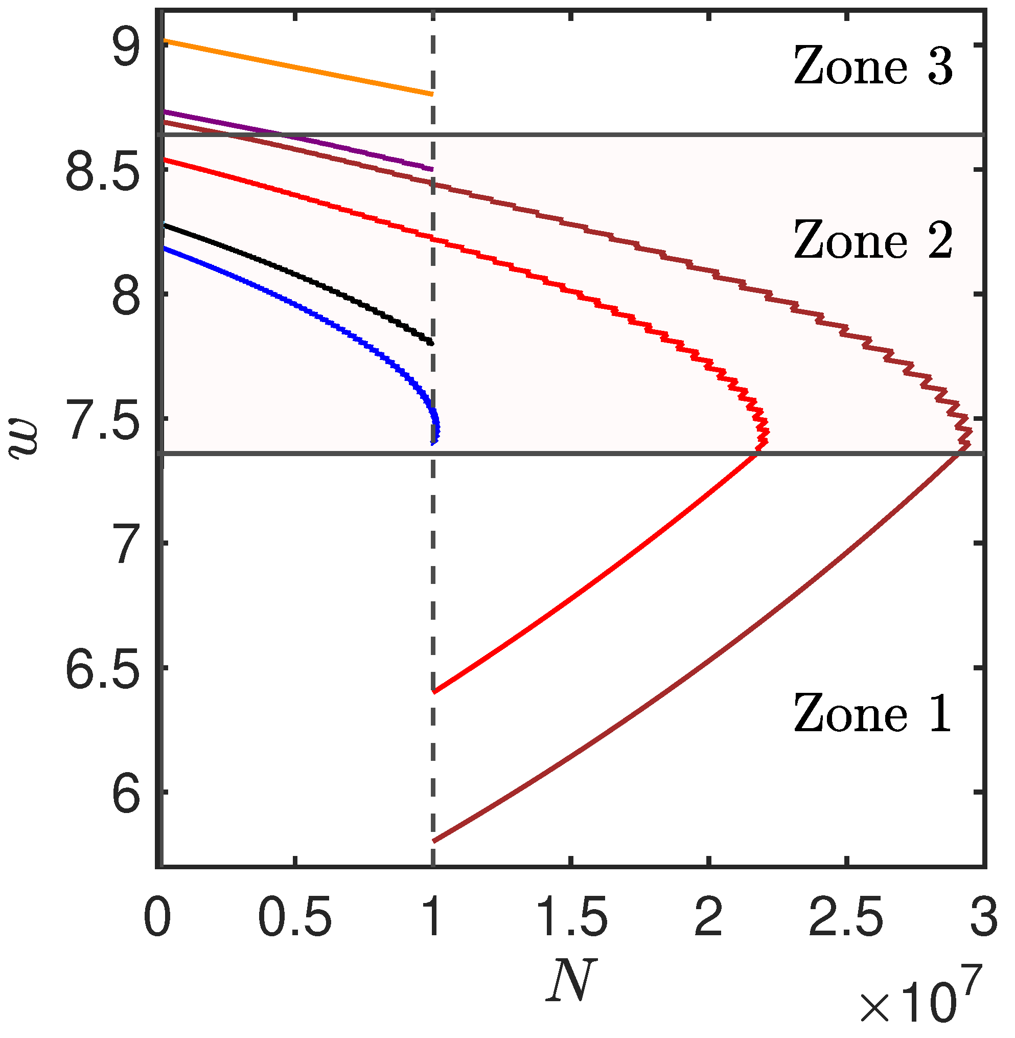
Key features in the N w plane are the initial line N = N 0 , the termination line w = r N , and three horizontal zones corresponding to different control strategies (Figure 2):
  • zone 1:  w < 1 α d : The control u = 0 , and the number of cancer cells undergoes logistic growth;
  • zone 2:  1 α d < w < 1 + α d : The control switches between one and zero depending on if w > h ( t ) or w < h ( t ) . This area is called the “switching zone”; since h ( t ) is periodic, there will typically be two switches per day;
  • zone 3:  w > 1 + α d : The control u = 1 , and the tumor size decays in a manner in accordance with logistic dynamics.
Since w increases monotonically, solutions can move through zones 1 to 2 and 2 to 3. In zone 1, N increases monotonically; in zone 2, switching occurs (u is either 0 or 1); and in zone 3, N decreases monotonically. In zone 2, the duration of drug administration increases as w increases; hence, there is a shift in net tumour growth near the boundary with zone 1 to net tumour decay for higher w. Trajectories start on N = N 0 and terminate on the termination line w = r N .
We denote with N b = 1 + α r d and N a = 1 α r d the tumor size at the intersection of the termination line with the upper and lower bounds of the switching zone, respectively, (i.e., with w = 1 + α d and w = 1 α d ). The phase planes are different depending on the initial tumour size relative to N a , N b , yielding three cases: large, intermediate, and small initial tumour sizes, Case A ( N 0 > N b ), Case B ( N b > N 0 > N a ), and Case C ( N 0 < N a ), respectively, Figure 2. In cases B and C, trajectories can start above the termination line; trajectories cannot start in zone 3, above the termination line (nor in zone 2, with a value of w 0 that is sufficiently high), since the tumour decays and the trajectory fails to reach the termination line. All trajectories in the switching zone are aperiodic, with the fraction of the day when the drug is administered increasing as the treatment progresses.
The aperiodic behavior of the control function u is due to the fact that the time intervals in which w ( t ) > h ( t ) increase because w strictly increases with time. In the following, we analyse case A, N 0 > N b , illustrated for a fixed set of parameters. There are six types of trajectories (Figure 3). In Figure 4, an example of a type-3 trajectory, with an initial tumour size of 0.1 K ( K = 10 8 cells), is shown, illustrating the increase in the proportion of the day when MTD is applied and the daily reduction in tumour size over time.
The cost of the optimal solutions can be evaluated. For a N w trajectory with v switching times ( t ^ 1 , t ^ 2 , . . . , t ^ v ), the cost function, J, Equation (1), can be expressed as follows:
J N 0 , w 0 = r N ( T ) + i = 0 v u i t ^ i t ^ i + 1 ( 1 α cos ( 2 π t ) ) d t
where t ^ v + 1 = T , t ^ 0 = 0 , and u i is the value of control for t ( t ^ i , t ^ i + 1 ) . This can be easily evaluated to obtain an analytic cost.

The Cost and Treatment Time of Optimal Solutions

We explore the optimal solutions for an initial tumor size of 0.1 · 10 8 cells (with a carrying capacity of 10 8 cells) using a grid in w 0 , with steps of 0.002 in w 0 , where w 0 [ 0.002 , 500 ] (the upper bound is the maximum possible value of r N 0 ). For each solution, starting at ( N 0 , w 0 ) , we calculate the horizon time T ( w 0 ) and its cost J ( w 0 ) (we drop dependence on N 0 for simplicity, as it is kept fixed). The horizon time T ( w 0 ) and cost J ( w 0 ) are shown in Figure 5, colour coded by the type of trajectory, as shown in Figure 3. The cost is broken down into its two components; the running cost dominates for low w 0 , with a high horizon time T, and the terminal cost dominates for high w 0 , with low horizon times.
The time horizon T as w 0 0 , because the trajectory spends an increasing (arbitrary) amount of time close to w = 0 , whilst T 0 as w 0 r N 0 .
The lowest cost is achieved for a type-3 trajectory; trajectories with sections in zone 1 are typically costly because of the growth phase of the tumour, whilst type 2, which also has a net growth phase, can also be costly. In effect, these growth phases allow the horizon time T for these trajectories to increase.
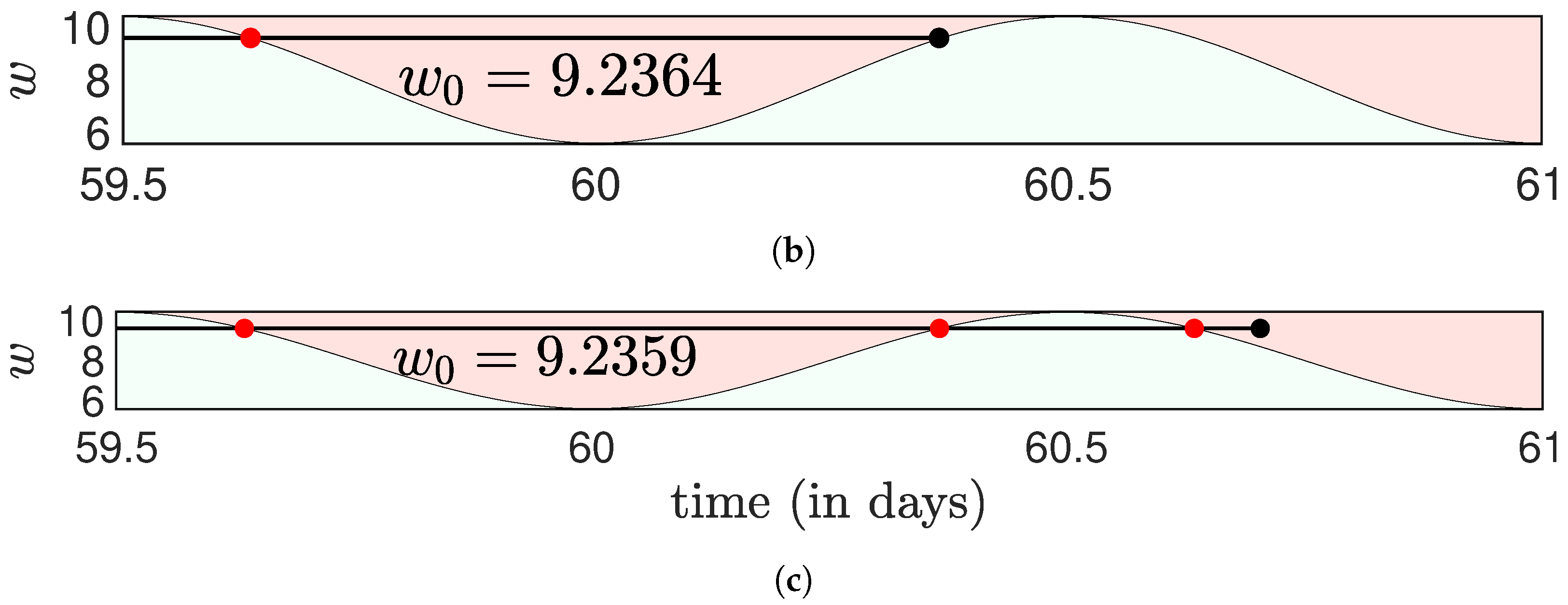
The cost, Equation (16), around the minimum is shown in Figure 6; these are type-3 solutions (for these parameter values). There are clear trends throughout the day with approximate fine-scale harmonic time dependence. However, there are discontinuities in J ( w 0 ) , which manifest as gaps in the horizon time T ( w 0 ) ; i.e., there are no solutions in our set for some values of T, as shown in Figure 6. Since the optimisation problem of minimising J, subject to the ODE dynamics expressed in Equation (7), can be solved, an optimal solution exists for every value of the horizon time T. Therefore, our set of solutions, Figure 4a, is incomplete. An examination of the trajectories ( N ( t ) , w ( t ) ) across a discontinuity, i.e., comparing trajectories with w 0 values lying across a discontinuity, demonstrates that the value of w upon termination jumps across the function h ( t ) , retaining u = 1 at termination, as shown in Figure 7, resulting in a jump in the horizon time T. This suggests that the missing solutions must terminate in the skipped region with u = 0 . These solutions, in fact, correspond to trajectories that cross the termination line without terminating; PMP requires that solutions satisfy the transversality condition upon termination; termination on the first crossing is not a requirement. Therefore, our missing solutions are in fact extensions of existing solutions, as shown in Figure 3. Specifically, certain trajectories can continue past the termination line in zone 2 and undergo a switching event that allows a second (or higher number of) crossing(s) of the termination line, as shown in Figure 8a. The discontinuities in the cost and time horizon for the first-crossing terminating solutions, as shown in Figure 6 and Figure 7, occur when the trajectory terminates at a switching time. Trajectories that cross the termination line an even number of times end in regions where u = 0 , whereas trajectories that cross the termination line an odd number of times end in regions where u = 1 . For the parameter values considered, trajectories that intersect the termination line up to three times are required to fill the gaps; the time horizon, T, is shown as a function of w 0 in Figure 8b, colour-coded by the number of crossings of the termination line. The time horizon is tri-valued for multiple intervals in w 0 . In Figure 9, the cost is shown as a function of w 0 for 9.2 w 0 9.95 (panel a), and as a function of the time horizon for 46.35 T 61.18 (panel b), showing detail around the minimum cost solution in T. There is continuous dependence of the cost on w 0 since the trajectories of two and three crossings form two intersecting branches that connect the previously observed discontinuities. These extended trajectories are of lower efficacy than trajectories that start from the same w 0 value but terminate on the first crossing of the termination line.

5. Gompertz Model

In this section, the cost function in Equation (1) is minimised, subject to the tumour having Gompertz growth dynamics [41]:
d N d t = g N log λ N + ε d u N .
Here, u is the drug intensity, N is the number of cancer cells, g is the Gompertz growth rate of the cancer cell population, and d is the drug-induced death rate (at MTD, u = 1 ). λ and ε are positive parameters discussed in the subsequent paragraphs.
Our model for Gompertz growth reduces to exponential growth at a rate of g log ( λ / ε ) when N < < ε and approaches the more typical form for Gompertz growth dynamics (with ε = 0 ) [42] at a large N. With ε = 0 , the growth rate as N 0 , so tumours can never be eliminated. When u is constant, there are two fixed points: N 1 * = 0 and N 2 * = λ exp d u g ε . In particular, in the absence of a drug, the capacity is N 2 = λ ε , a stable positive fixed point when λ > ε , whilst N 1 * is unstable. Thus, we assume 0 < ε < λ . We assume the initial tumor size is smaller than the capacity N 2 * . When u > 0 and constant, the nontrivial fixed point is N 2 * = λ exp d u g ε . A transcritical bifurcation occurs when g log λ ε d u = 0 , so N 1 * is stable when N 1 * > N 2 * , i.e., when d u > g log λ ε . Thus, we assume that d > g log λ ε , so the tumor can be eliminated at MTD.
In the following, PMP is employed in order to minimise the cost functional for a fixed time horizon T, subject to the tumor dynamics given by Equation (17). The Hamiltonian of the system is
H [ N , p , u , t ] = p g N log λ N + ε + d p N + 1 α cos ( 2 π t ) u
and it is linear with respect to u. Thus, there exists a switching function:
Φ [ N , p , u , t ] = d p N + 1 α cos ( 2 π t )
which is identical to the switching function in the logistic model. By introducing the variable w = N p , the switching function takes the following form:
Φ [ N , w , t ] = d w + 1 α cos ( 2 π t ) = d ( w h ) .
The transversality condition is p ( T ) = r , which yields, in terms of N and w, the termination line:
w ( T ) = r N ( T )
The adjoint variable p has the following dynamics:
d p d t = H N = p g log λ N + ε + p g N N + ε + d u p
which, through Equation (17), gives the following dynamic equation for w:
d w d t = g N N + ε w
We thus have a nullcline at w = 0 ; then, since w ( T ) is positive, as shown in Equation (19), it follows that w strictly increases and all dynamics take place in the first quadrant.
Based on the theorem in Section 3.1, the optimal solutions are bang–bang since minimising singular solutions do not exist. Specifically, singular solutions are of order 1 since
u d 2 H u d t 2 = d 2 g ε N w ( N + ε ) 2 ,
but to be a minimum, this would have to be negative based on the LC conditions, which is not possible, as w is positive.
As with the logistic model, when w ( t ) > h ( t ) , u ( t ) = 1 , and when w ( t ) < h ( t ) , u ( t ) = 0 , where h ( t ) = 1 α cos ( 2 π t ) d . The ( N , w ) plane is again divided into three zones:
zone 1: 
Here, w is less than 1 α d ; the control is equal to zero, and the tumor size increases.
zone 2: 
Here, 1 α d < w < 1 + α d ; the control switches between one and zero.
zone 3: 
Here, w is greater than 1 + α d ; the control is equal to one, and the tumor size decreases.
There is no analytical solution to the Gompertz model for a constant u, as indicated by Equation (17); thus, to find solutions, we numerically solve the evolution equations for N and w. Specifically, starting from an initial point N 0 , w 0 , we numerically integrate the ODEs stopping when either the switching function changes sign, i.e., when w = h is reached and the control switches, or when the termination line is reached, so the transversality condition is satisfied. The numerical integration then continues (recording that event) until the next stopping event. This is repeated until the termination line is reached, either on the first or a later crossing.
We illustrate the types of solutions for the following parameters: ε λ = 1 3 , g = 0.025 per cell, d = 0.1373 per cell, r = 5000 · 10 8 cells per day, and α = 0.3 . The initial tumour size is 10 7 cells, and the carrying capacity is 10 8 cells. The phase space is displayed in Figure 1. The same trajectory categories are found as in the logistic model, with trajectories that begin and terminate in the switching zone (type-3 trajectories) having the lowest cost (including minimised over T), as shown in Figure 10. As in the case of the logistic model, we need to include trajectories that intersect the termination line up to three times. Figure 11a shows the dependence of the cost on w 0 . As in the logistic model, there exist oscillatory patterns in the cost function; these patterns are due to the dynamics of the w N trajectories close to termination (Figure 11).

6. Aperiodic Solutions in Multi-Compartment Models

Solid tumours are not typically homogeneous, showing heterogeneity in both architecture and genome. Multi-compartment models can be used to capture this heterogeneity. Let N ( t ) be the density vector in an n-compartment model and all components be non-negative, with interconnected dynamics, as follows,
d N d t = g N u d N ,
with a net tumour cell growth rate matrix g and a drug-induced death matrix d (with non-negative entries), which are not necessarily diagonal since death can occur during transfer as in cell cycle models [43]. In general, g encodes differentiation and growth and naturally splits into growth/differentiation and native death, with g = g + + g . The native death rate matrix is diagonal with non-positive entries. The growth/differentiation matrix g + will satisfy i g i j + 0 . The matrix g u d will have negative diagonal entries and non-negative off diagonal; the first orthant is thus a positive invariant [29]; i.e., if N i ( 0 ) > 0 , then N i ( t ) > 0 for all of time t > 0 .
We minimise the generalised cost function (c.f (1)),
J [ N , u ] = r · N ( T ) + 0 T h ( t ) u ( t ) d t
where the terminal cost generally depends on all compartments, r i 0 , and we remove the d prefactor in the running cost (only included previously to simplify expressions). We illustrate solutions with h ( t ) = ( 1 α cos ( 2 π t ) ) , removing the factor of d 1 .
To apply PMP, we introduce the costate variables p and construct the Hamiltonian:
H = i j p i g i j N j u i j p i d i j N j + h u .
The switching function thus has the following form:
Φ = i j p i d i j N j + h
and the costate variables have the following dynamics:
d p d t = g T p + u d T p ,   with   p ( T ) = r .
Thus, the costates terminate with non-negative values. Since the matrix g T + u d T will have positive diagonal entries and non-positive entries off-diagonal, the first orthant of the adjoint system is negatively invariant; i.e., if p i ( T ) > 0 , then p i ( t ) > 0 for all t < T . So, both N and p are positive.
We conclude that
d d t p T d N = p T [ d , g ] N ,
so if d commutes with g , the combination p T d N is constant. Assuming [ d , g ] = 0 , we then have
d Φ d t = d h d t .
Hence, if there is a switching point at t 1 , i.e., Φ ( t 1 ) = 0 , then there is periodic switching since Φ ( t 1 + τ ) = Φ ( t 1 ) , where τ is the period of h. A special case is if the drug acts equally on all compartments, i.e., d = d I , with I being the identity matrix. The dynamics are then effectively a one-compartment dynamic along the growth eigendirection ζ , i.e., g ζ = λ ζ , with λ being the largest eigenvalue of g . This follows since the direction ζ dominates and all other directions that are diluted out during both growth and whilst the drug is applied (observe that g u d I have the same eigenvectors for all u).
In general, there is differential death amongst compartments, for instance, both in cell cycle models [43], and heterogeneous tumour models (with compartments of differing sensitivity to the drug) [44]. Then, [ d , g ] 0 , and the bang–bang solution is not necessarily periodic as periodicity would require that p T d N is also periodic. So, periodic solutions are an exception since they only occur when additional constraints are imposed.
We numerically explore a two-compartment cell cycle phase model. The cell cycle is divided into four phases, the growth phase (gap phase 1, G1), DNA synthesis (S), a second (normally shorter) growth (gap) phase (G2), and mitosis (M), where the duplicated chromosomes descend to two daughter cells and the cell physically divides into two cells. Many anti-cancer drugs target cell division. Models that incorporate these phases have been developed [29,43], including a number of linear compartment models [43]. The simplest is a two-compartment model, comprising non-dividing cells N 1 ( t ) (compartments G1, S, and G2) and actively dividing cells N 2 ( t ) (in M phase). The dynamics can be obtained as follows:
d N 1 d t = a 1 N 1 + 2 ( 1 u ) a 2 N 2 , d N 2 d t = a 1 N 1 a 2 N 2 ,
where the compartment transfer rates are a 1 , a 2 , and u ( t ) is the drug concentration with a maximal tolerated dose (MTD) rescaled to 1. The drug is assumed to kill actively dividing cells, and it is 100% efficacious at MTD.
The matrices above are thus
g = a 1 2 a 2 a 1 a 2 , d = 0 2 a 2 0 0 , [ d , g ] = 2 a 2 a 1 a 1 a 2 0 a 1
Thus, [ d , g ] 0 , and switching occurs when Φ = 0 or 2 a 2 N 2 p 1 = h . Thus, switching is possible if ( 2 a 2 ) 1 p 1 N 2 ( 2 a 2 ) 1 , which defines the switching zone. There are thus only periodic solutions with a daily period ( τ ) if N 2 p 1 periodically is equal to h * / ( 2 a 2 ) for some h * ( 1 , 1 ) ; in fact, there must be two switches per day. We have
d Φ d t = d h d t 2 a 2 a 1 p 1 N 1 + ( a 1 a 2 ) p 1 N 2 a 1 p 2 N 2
which can be of either sign. Thus, multiple switches can occur, and periodic drug regimens are not necessarily optimal since that requires that a 2 N 2 p 1 satisfies a periodicity condition. Using the generalised LC conditions, it can be shown that optimal solutions can only be of the bang–bang type, as shown in Appendix D.
To investigate the periodicity of optimal solutions in this model, two drug regimens are compared:
  • A drug regimen that satisfies PMP, hereafter referred to as PMP drug regimen (PMPDR);
  • A drug regimen that minimises the objective function when restricted to bang–bang periodic solutions and a period of one day. This solution is hereafter referred to as the optimal periodic drug regimen (OPDR).
The PMPDR and OPR solutions are determined numerically; details on the construction of the PMPDR solution are given in Appendix D. A time horizon of 1 year is used, and the initial number of cancer cells is 10 8 . The growth rates of the dividing and non-dividing cancer cell populations, a 1 and a 2 , were taken from [45]. The fraction of dividing over non-dividing cells at the start of the therapy is N 1 ( 0 ) N 2 ( 0 ) = 1 / a 1 1 / a 2 . Finally, to define the objective function, we assume r 1 = 52.6 and r 2 = 31.2 , conditions that were arbitrarily chosen; see Appendix D for more information.
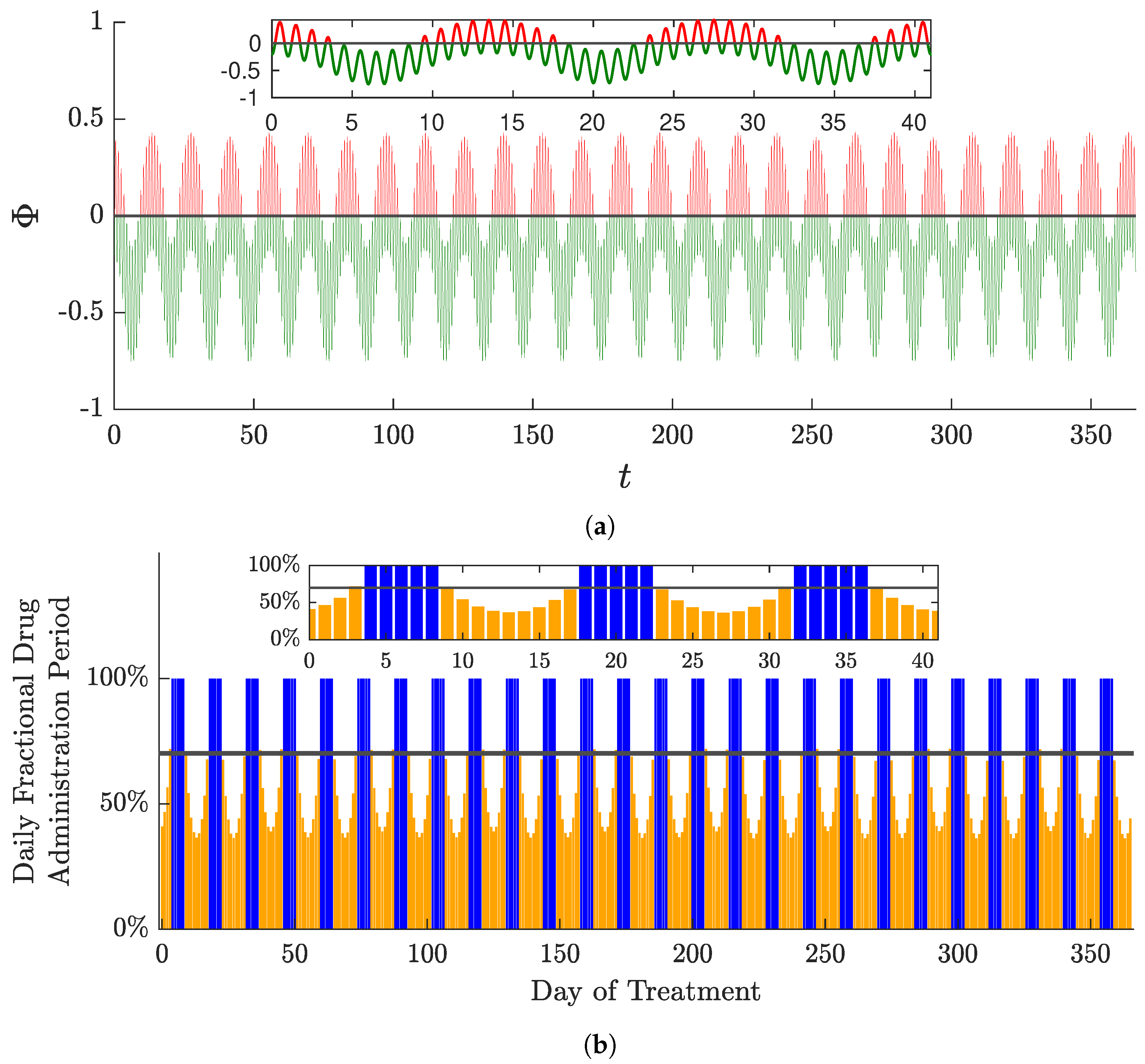
The switching function under PMPDR is quasi-periodic with two periods—a fast period around 24 h (expected because of h) and a slower period of 14 days, as shown in Figure 12a. This results in a treatment schedule comprising alternating intervals of MTD for a few days interspersed with a few days with daily chronotherapy, with the duration of infusion ranging from a minimum of around 9 h mid-interval to a minimum of 8 h 50 min and a maximum of 9 h 50 min ( 36 % and 41 % , respectively, of the day), as shown in Figure 12b. The average drug concentration over the time horizon is 0.0223 , lower than that in the optimal periodic solution, resulting in lower toxicity (running cost); 227.6308 under PMPDR and 228.5683 under OPDR. The tumour size has a decreasing trend throughout the therapy, reaching approximately 0.0762 cells by the end of the treatment, with N 1 ( T ) = 0.0497 and N 2 ( T ) = 0.0264 , as shown in Figure 13.
Although PMPDR is not necessarily optimal (PMP is not a sufficient condition), the value of the payoff under PMPDR ( J PMPDR = 231.0688 ) is smaller than the value of the payoff under PODR ( J PODR = 232.2599 ); consequently, in this example, optimal solutions are not periodic. PMPDR has lower total drug toxicity compared to PODR (the running cost under PMPDR is approximately 227.6308 , and the running cost under PODR is approximately 228.5683 ), whereas the terminal tumour sizes are similar, with N 1 ( T ) + N 2 ( T ) = 0.0762 and 0.0838 for PMPDR and PODR, respectively.

7. Conclusions

Here, we proved for one-compartment tumour growth models that optimal chronotherapy is typically aperiodic and bang–bang, with the daily duration of MTD treatment increasing over time, possibly extending to the full 24 h. Singular arcs do not exist for either logistic or Gompertz tumour growth models; for singular arcs to exist, the cellular replication rate g ( N ) must satisfy d 2 g d N 2 > 0 , as for instance, in the case of the surface model, where d N d t = a N + b d N [41]. Solutions are periodic only for the simplest of dynamic models, exponential growth in the case of cytotoxic drugs (Appendix A), and in the absence of natural cell death ( d 0 = 0 ) for cell cycle drugs. For the logistic and Gompertz growth models, we categorised the family of optimal solutions. Solutions were naturally visualised in the phase plane; however, to obtain a complete set of optimal solutions across all time horizons, solutions that cross the termination line multiple times must be included.
To illustrate the advantage of aperiodic bang–bang solutions over periodic the administration of chemotherapy drugs, we compared optimal solutions (optimised in terms of both time horizon T and drug administration strategy u) with corresponding optimal solutions that are constrained to be periodic, referred to in the following as unconstrained and constrained optimal solutions, respectively. We used the Gompertz growth model (Equation (17)), with parameters estimated from experimental mice data [42]. A sensitivity analysis on the parameters d and r showed that the unconstrained system had high sensitivity to d whilst being nearly insensitive to the parameter r across orders of magnitude of the initial tumour sizes N 0 , as shown in Appendix E. We thus compared optimal solutions for tumours with a low drug-induced death rate, ( d = 1.19 days−1), referred to as low-susceptibility tumours, and tumours with a high drug-induced death rate ( d = 2.41 days−1), or high-susceptibility tumours. A low-sensitivity tumour comprising 10 6 cells would be eliminated within two months of continuous MTD, which can be compared to a figure of 9.5 days for a high-susceptibility tumour.
For low-susceptibility tumours ( d = 1.19 days−1), the constrained optimal solutions are continuous MTD for all tumour sizes. The unconstrained optimal solutions are identical to those of the constrained problem (i.e., MTD) for N 0 10 7 , while for larger tumours, N 0 > 10 7 , a bang–bang strategy is optimal with an initially aperiodic u which then changes to continuous MTD until the end of the treatment (Figure 14).
Characteristics of these optimal solutions are compared in Figure 15. As expected, the duration of treatment T is longer under aperiodic treatment (compared to continuous MTD), while the terminal tumour size is similar, around 10 3 cells for all initial tumour sizes, as shown in Figure 15a,c; hence predicting elimination of the tumour (in absence of emergence of resistance). Total drug administered over the treatment is in fact higher for the aperiodic solution compared to continuous MTD, but the toxicity to normal cells is lower for the larger tumour sizes, as shown in Figure 15d,f. The gains of the aperiodic solution are small for low-susceptibility tumours, with the reduction in normal cell toxicity being less than 2 % relative to MTD. Optimal periodic solutions do not exist.
For high-drug-susceptibility tumours ( d = 2.41 per day), the constrained optimal solutions are periodic for all tumour sizes investigated, whilst the aperiodic solutions have a daily infusion period of <24 h for all tumour sizes, as shown in Figure 14c,d. For high-susceptibility tumours, we compare the optimal constrained and unconstrained solutions and continuous MTD, as shown in Figure 16. All solutions led to a final tumour size of below 10 3 cells, as shown in Figure 16a, again predicting the elimination of the tumour. Aperiodic solutions tend to have lower running costs than periodic solutions, with the difference increasing with larger tumours, as shown in Figure 16b. MTD solutions have the highest running cost among the three types. As expected, the duration of treatment T is longer for periodic and aperiodic solutions, and the total amount of drug used is higher compared to MTD. For large tumours, aperiodic solutions have substantially lower drug use per day compared to periodic solutions, as shown in Figure 16e, explaining the longer treatment durations T. Optimal aperiodic solutions demonstrate improvements over periodic chronotherapy: the toxicity to normal cells is reduced by as much as 8.5 % , as shown in Figure 16, for large tumours. As expected, both periodic and aperiodic solutions exhibit significant reductions in toxicity in comparison to MTD solutions, with a reduction of 20 % for the unconstrained solution for the largest tumour.
Here, we proved that optimal chronotherapy solutions for one-compartment non-linear growth tumour models are aperiodic. Periodic bang–bang solutions with a diurnal period, in fact, appear to be the exception, occurring in one-compartment linear growth models, as shown in Appendix A, and n-component linear growth models in special cases, as noted in Section 6. Our objective function weighed the competing demands of minimising the terminal tumour size against the drug’s toxicity to normal cells, a toxicity that was circadian-phase-dependent. Our aperiodic solutions applied drugs at times when normal cells had low drug susceptibility, increasing the daily infusion duration as treatment progressed. When also minimised over the horizon time solutions, the optimal solution could be Type 3, 4, or 5, as shown in Figure 3, depending on the initial tumour size and drug efficacy, i.e., comprising a possible aperiodic chronotherapy initial section and a possible continuous MTD final section. During chronotherapy, the drug application interval is long enough to always decrease tumour size.
Our results are robust to model structure. Firstly, the results were obtained under conditions of including a running cost that is linear with respect to tumour size, modelling, for instance, the risk of metastasis or mutation, see Appendix F. Secondly, n-compartment linear growth models also generically have aperiodic solutions, as shown in Section 6. So, although we used simple cancer growth models to enable a thorough analysis of the existence of periodic solutions, the only case where periodic solutions are standard appears to be a one-compartment linear growth model (exponential growth), as shown in Appendix A; generalisations (considering nonlinearity and multiple compartments with differential drug-induces death amongst compartments) lead to aperiodic solutions, as shown in Section 6. We hypothesise that periodic optimal solutions with a daily period are in fact exceptions (for the harmonic cost objective), and optimal chronotherapy solutions are generically aperiodic. Further work is required to verify this hypothesis for more complex cancer models under the cost function (1), for instance, in spatial cancer models or structured growth models [26,46,47,48,49,50,51,52,53] and models incorporating drug pharmacokinetics/pharmacodynamics [31,46,54,55]. For ODE compartment models, similar methods of analysis can be used to determine analytically or numerically solutions that satisfy PMP (necessary conditions). PDE models of cancer growth would require optimisation methods for PDEs (distributed parameter systems), for instance, discretisation methods [56], or extensions of control theory to infinite-dimensional spaces [57].

Author Contributions

Conceptualization, B.D.E.T. and N.J.B.; formal analysis, B.D.E.T. and N.J.B.; methodology, B.D.E.T. and N.J.B.; software, B.D.E.T.; supervision, N.J.B.; validation, B.D.E.T. and N.J.B.; writing—original draft, B.D.E.T. and N.J.B.; writing—review and editing, B.D.E.T., A.B. and N.J.B. All authors have read and agreed to the published version of the manuscript.

Funding

Byron D. E. Tzamarias received funding from the Engineering and Physical Sciences Research Council (grant number 2441135).

Data Availability Statement

The data is available from the authors on request.

Acknowledgments

All numerical evaluations and graphics were generated using Matlab R2023a.

Conflicts of Interest

The authors declare no conflicts of interest. The funders had no role in the design of the study; in the collection, analyses, or interpretation of data; in the writing of the manuscript; or in the decision to publish the results.

Appendix A. Optimal Solutions for the Exponential Growth Model

In this section, the cost function (1) is minimized for a fixed time horizon T, subject to the exponential tumor growth dynamics:
d N ( t ) d t = λ d u ( t ) N ( t ) , N ( 0 ) = N 0 ,
where λ is the (net) growth rate of the cancer population in absence of the drug. The parameter d is the drug-induced death rate of cancer cells when the drug is at maximum tolerated dose (MTD, u = 1 ); we assume d > λ in order for the treatment to be effective; i.e., the tumour decreases in size under MTD.
To apply PMP, we created the following Hamiltonian:
H [ N , u , p , t ] = λ d u N p + 1 α cos ( 2 π t ) u
with p being the costate. PMP was slightly modified because of the explicit time dependence (from the running cost kernel), as noted in Appendix B. An additional state variable s was introduced, with dynamics d s d t = 1 , s ( 0 ) = 0 , and a costate of q, yielding the Hamiltonian
H ˜ N , s , u , p , q = λ d u N p + q + 1 α cos ( 2 π s ) u ,
which has identical partial derivatives in q , N , u to those of H. The adjoint equation is thus as follows:
d p d t = H ˜ N H N = ( λ d u ) p
so variable s and costate q can be ignored. The only caution is that H is not constant as would normally be the case. The transversality condition is
p ( T ) = l N | N = N ( T ) = r
where l [ N ] = r N is the terminal cost.
The switching function is given by
Φ [ N , t ] = H u = d N p h ( t ) , w i t h h ( t ) = 1 α cos ( 2 π t ) d .
We set variable w N , p = N p , and from Equations (A1) and (A2), we found that d w d t = 0 . Thus, w is constant, and since h is a harmonic function, the switching function Φ = d w h ( t ) is harmonic. Hence, there are no singular solutions, and the optimal solutions are of the bang–bang type. Specifically, when h is greater than w, the control is u = 0 , and when h is smaller than w, the control is u = 1 . There are three possible types of optimal solutions based on possible values of the constant w:
I. 
Large tumours. Case: w > 1 + α d h ( t ) . The switching function is negative, so treatment comprises MTD for the full horizon, u = 1 , giving N ( T ) = N 0 exp ( λ d ) T from Equation (A1). Thus, w = N ( T ) p ( T ) = r N 0 exp ( λ d ) T > 1 + α d , giving the tumour size constraint
N 0 > e ( d λ ) T 1 + α d r .
II. 
Small tumours. Case: w < 1 α d h ( t ) . The switching function is positive; therefore, u = 0 for the full horizon, and we have N ( T ) = N 0 exp λ T , and thus w = N ( T ) p ( T ) = r N 0 exp λ T 1 α d , giving the tumour size constraint
N 0 < e λ T 1 + α d r .
III. 
Intermediate-sized tumours. Case: 1 α d w 1 + α d . In this case, the control switches from 1 to 0 and vice versa. Let t 1 , . . . t n be the switching times in increasing order. Observe that Φ ( 0 ) = d w + 1 α < 0 , and so u ( 0 ) = 1 ; then, by solving for t k , k = 1 , . . n , the equation Φ ( t k ) = 0 becomes
cos ( 2 π t k ) = d w 1 α
with a first switching time of t 0 = 1 2 π cos 1 1 w d α . Drug administration is periodic thereafter until T, with the drug being administered around noon between k + [ t 0 , t 0 ] 0 < k < T , and, on the last day zero beyond t = T . The tumour size decays by e λ 2 d t 0 per day, so it decays if 2 t 0 > λ / d . By taking the limits t 0 0 and t 0 0.5 , we can obtain the initial tumour size range for this case between that of small and large tumours as defined above.

Appendix B. The Pontryagin Minimum Principle for Non-Autonomus Systems

We use the following formulation of PMP for non-automous systems:
Theorem A1. 
Consider the control of x ( t ) R n subject to the dynamics
d x ( t ) d t = f x ( t ) , u ( t ) , t , 0 t T , x ( 0 ) = x 0 ,
where the control u ( t ) is valued in the set U R m . The optimal control u ( t ) , and the path x ( t ) that maximises the pay-off,
J [ x , u ] = g ( x ( T ) ) + 0 T r ( x ( t ) , u ( t ) , t ) d t ,
is given by
d x ( t ) d t = p H ( x , u , p , t ) | x ( t ) , u ( t ) , p ( t ) , d p ( t ) d t = x H ( x , u , p , t ) | x ( t ) , u ( t ) , p ( t ) ( costate dynamics ) p ( T ) = x g ( x ) | x ( T ) ( transversality condition ) u ( t ) = argmax u U H ( x ( t ) , u , p ( t ) , t ) ( local maximisation ) ,
where p ( t ) R n is the costate and H ( x , u , p , t ) = r ( x , u , t ) + p f ( x , u , t ) is the Hamiltonian.
Here, x , p are partial derivatives with respect to x , p , respectively, in vector form.
Proof. 
This follows from the standard maximum principle as follows. Define the extra variable y with d y d t = 1 , y ( 0 ) = 0 ; i.e., solution y ( t ) = t . Then, the combined ( x , y ) system is autonomous, with equations
d x ( t ) d t = f ( x ( t ) , u ( t ) , y ( t ) ) , d y d t = 1 , 0 t T , x ( 0 ) = x 0 , y ( 0 ) = 0 .
and a cost/pay-off of
J [ x , y , u ] = g ( x ( T ) ) + 0 T r ( x ( t ) , u ( t ) , y ( t ) ) d t .
Using (the autonomous) PMP, the Hamiltonian thus reads
H ˜ ( x , y , u , p , q ) = r ( x , u , y ) + p f ( x , u , y ) + q = H ( x , u , p , y ) + q ,
with H given in the theorem and using q for the costate of variable y.
This yields costate dynamics,
d q d t = d p d t r + p f ,
with transversality condition q ( T ) = 0 .
Upon substituting y ( t ) = t into Hamiltonian’s equations for x , p , we obtain
d x ( t ) d t = p H ˜ p H ( x , u , p , y ) | x ( t ) , u ( t ) , p ( t ) , y = t , d p ( t ) d t = x H ˜ x H ( x , u , p , y ) | x ( t ) , u ( t ) , p ( t ) , y = t ( costate dynamics ) p ( T ) = x g ( x ) | x ( T ) ( transversality condition )
as required. The control u is given at time t by
u ( t ) = argmax u U H ( x ( t ) , u , p ( t ) , y ( t ) ) + q ( t ) argmax u U H ( x ( t ) , u , p ( t ) , t ) ( local maximisation ) .
Hence, the autonomous PMP is as stated. □

Appendix C. Accuracy of Numerical Calculation
To allow the logistic model to evaluate the switching times, the following transcendental equation was solved numerically by employing a Newton-type method,
1 α cos ( 2 π t ) d = w i 1 λ ρ N i 1 exp ρ ( t t i ) .
In the Gompertz model, no analytical solutions are known and therefore we used numerically evaluated solutions. The switching and termination points were evaluated via event location in Matlab.
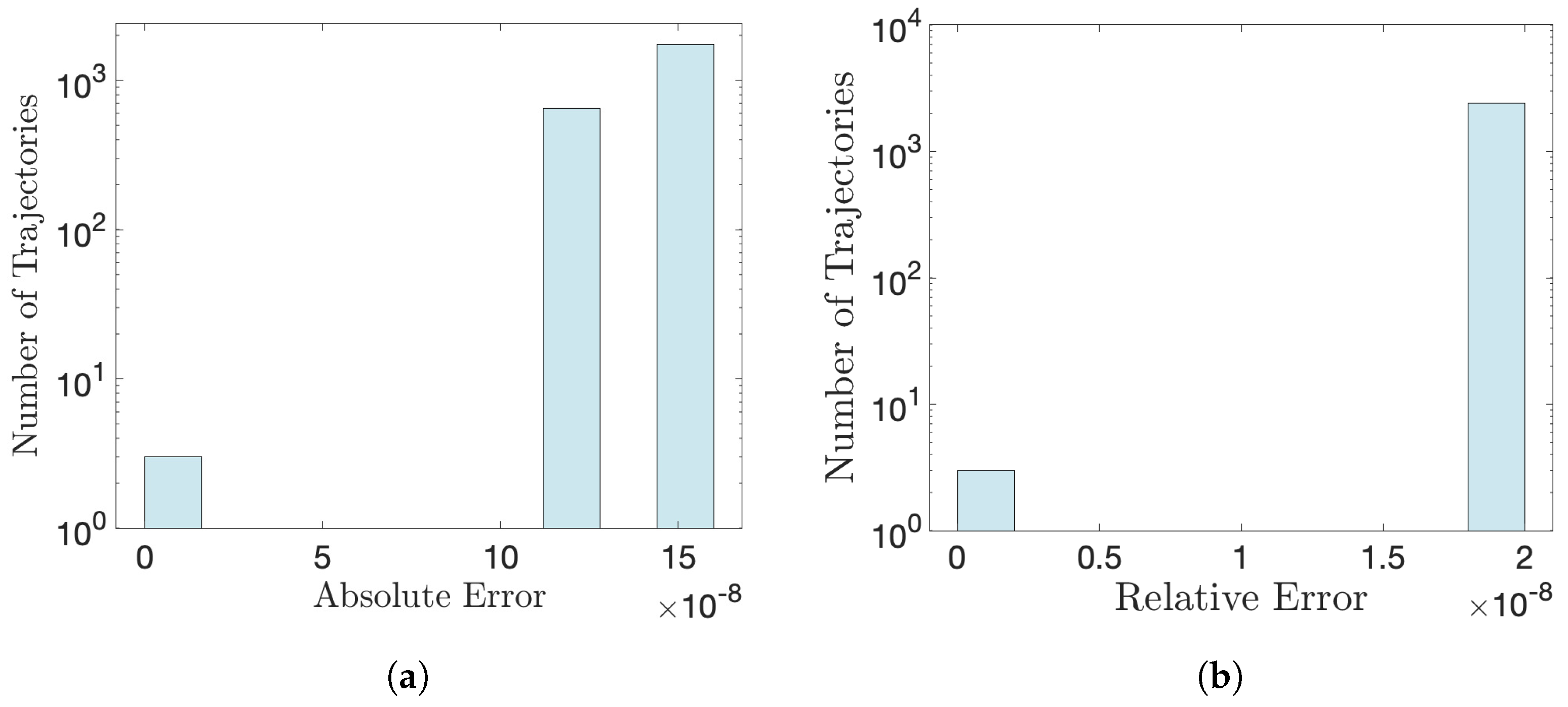
For every optimal solution, we define the two absolute errors w ( t s ) h ( t s ) (where t s is a switching point) and w ( T e ) r N ( T e ) (where T e is a termination point) and the relative errors w ( t s ) h ( t s ) max w ( t s ) , h ( t s ) and w ( T e ) r N ( T e ) max N ( T e ) , r N ( T e ) . The accuracy of an optimal solution is quantified by the maximum absolute error (and relative error) of all constituent switching and termination points. As illustrated in Figure A1, the numerical evaluations in both models achieved very high accuracy, with absolute and relative errors being of the order of 10 8 (for the Gompertz model) and 10 6 for the logistic model.
Figure A1. Estimated computational errors of the switching and termination times for the logistic and the Gompertz models. We define as the absolute error of a trajectory the maximum of the quantities h ( t 1 ) w ( t 1 ) , . . . , h ( t q ) w ( t q ) (where t 1 , . . . , t q are all switching times) and r N ( T ) w ( T ) , where T is the termination time. Similarly, the relative error of a trajectory is defined as the maximum of the quantities h ( t 1 ) w ( t 1 ) max ( h ( t 1 ) , w ( t 1 ) ) , , h ( t q ) w ( t q ) max ( h ( t q ) , w ( t q ) ) and r N ( T ) w ( T ) max ( r N ( T ) , w ( T ) ) . For both models, the absolute and relative errors of 2394 trajectories were evaluated. Panels (a,b): absolute and relative errors in the logistic model; panels (c,d): absolute and relative errors in the Gompertz model.
Mathematics 12 03516 g0a1aMathematics 12 03516 g0a1b

Appendix D. Multi Compartment Cell Division Model

In this Section, PMP is applied to investigate wether optimal solutions that minimise the cost functional expressed by Equation (22), with h ( t ) = ( 1 α cos ( 2 π t ) ) , subject to the tumour dynamics:
d N 1 d t = a 1 N 1 + 2 ( 1 u ) a 2 N 2 , d N 2 d t = a 1 N 1 a 2 N 2 ,
are periodic. The Hamiltonian is given by,
H = a 1 p 1 N 1 + 2 a 2 p 1 N 2 + a 1 p 2 N 1 a 2 p 2 N 2 2 a 2 u p 1 N 2
where p 1 and p 2 are the costates of the states N 1 and N 2 , respectively. p 1 and p 2 satisfy the adjoint equations and the transversality conditions:
d p 1 d t = a 1 ( p 1 p 2 ) , p 1 ( T ) = r 1 d p 2 d t = 2 a 2 p 1 + a 2 p 2 + 2 a 2 u p 1 , p 2 ( T ) = r 2
The switching function can be written as,
Φ = 2 a 2 w + h ,
with w = p 1 N 2 .
It can be shown that the optimal solutions are of the bang-bang type. Indeed, assuming that singular solutions exist, by employing the generalized LC conditions, it can be derived that singular solutions are of the order of 1 with
( 1 ) 1 u d 2 H u d t 2 = 8 a 2 2 a 1 w .
Since the switching function is equal to zero on a singular arc, w ( t ) = h ( t ) 2 a 2 > 0 . Consequently, ( 1 ) 1 u d 2 H u d t 2 < 0 ; thus, the singular solution cannot minimize the cost function, and so optimal solutions can only be bang–bang.
It can be shown that the control dynamics of trajectories that satisfy PMP can be expressed in terms of the closed system:
d w d t = a 1 a 2 + a 1 ( z v ) w ,
d z d t = a 1 z 2 + a 2 a 1 z + 2 a 2 ( 1 u ) ,
d v d t = a 1 v 2 + a 2 a 1 v 2 a 2 ( 1 u ) ,
d N 2 d t = a 1 z a 2 N 2 ,
with z = N 1 N 2 and v = p 2 p 1 . The control is given by:
  • u ( t ) = 1 iff w ( t ) > h ( t ) 2 a 2 ,
  • u ( t ) = 0 iff w ( t ) < h ( t ) 2 a 2 .
When w ( t ) = h ( t ) 2 a 2 , the control is expressed as: u ( t ) = 1 sign ( d d t ( w ( t ) h ( t ) 2 a 2 ) ) . The transversality conditions can be expressed in terms of w, N 2 and v:
w ( T ) = r 1 N 2 ( T ) ,
v ( T ) = r 2 r 1 .
All trajectories that satisfy Equations (A8)–(A11), with v ( T ) > 0 and u ( t ) = sign ( w ( t ) h ( t ) 2 a 2 ) , are admissible to PMP, for the cost functional J with weights r 1 = w ( T ) N 2 ( T ) and r 2 = r 1 v ( T ) . Examples in which optimal solutions are not periodic can be constructed by using the following approach:
  • Generate trajectories in the ( w , z , v , N 2 ) space (for a given time horizon T) using Equations (A8)–(A13)
  • Minimise the cost functional (1) with weights r 1 = w ( T ) N 2 ( T ) and r 2 = r 1 v ( T ) for drug regimens that are constrained to be periodic
  • Compare the cost of the generated ( w , z , v , N 2 ) trajectory to the optimised periodic drug regimen
Although PMP does not guarantee the optimality of the ( w , z , v , N 2 ) trajectory, it suffices to show that the optimised periodic drug regimen is suboptimal and thus optimal solutions are not periodic. For a complete proof, a similar analysis to the one conducted in Appendix E has to be conducted.

Appendix E. Realistic Parameter Analysis

Here, the behavior of the cost function for realistic parameter values is studied. Three case studies are presented: firstly, we consider the Gompertz tumour growth model (Equation (17)); secondly, we consider the exponential tumour growth model (Equation (A1)), where optimal solutions are periodic, as shown in Appendix A; and thirdly, we consider periodic optimal solutions of the Gompertz model; i.e., the optimal solutions are constrained to be periodic. The cost functional is minimized over both the time horizon T and drug administration u; hereafter, the minimum is referred to as ‘solution’. The growth rate as well as the carrying capacity of the tumour, in the Gompertz model, were taken from [42], where simple tumor growth models were fitted to murine data. The Gompertz model employed in [42] is expressed as follows d N d t = α exp ( β t ) N ; equivalently,
N = N 0 exp α β 1 exp ( β t )
differs from the Gompertz model employed in this work, which is given by Equation (17). Assuming that the parameter ϵ is much smaller than the initial tumour size N 0 , Equation (17) takes the form d N d t = g log λ N N and can be solved analytically giving the solution:
N = N 0 exp log λ N 0 1 exp ( g t ) ,
which is expressed as in Equation (A14). By equating the respective terms of Equations (A14) and (A15), the tumour growth parameters g and λ are given by g = β and λ = N 0 exp α β , where the initial tumour size N 0 was taken to be 10 6 cells in [42].
The growth rate of the exponential model was deduced by fixing the tumour size to zero in the Gompertz growth rate, i.e., log λ N + ϵ | N = 0 . The parameter ϵ was fixed to 10 4 , and it was assumed that the circadian clock had a strong influence on drug toxicity toward healthy cells, taking α = 0.95 . The value of the cancer cell death rate d depends on how the tumour responds to the drug. Finally, the value of r is subjective, weighting the two conflicting objectives of tumour elimination and low drug toxicity. Optimal solutions are studied for different values of r and d and initial tumour size N 0 .
In the unconstrained Gompertz model, we find that for low values of d, solutions are either MTD throughout the entire treatment horizon (when N 0 is large) or (when N 0 is smaller than a threshold) switch aperiodically on and off, subsequently turning into MTD, until the end of the treatment, as shown in Figure 14a,b. For high values of d, solutions are aperiodic, with drug administration switching on and off throughout the entire treatment, as shown in Figure 14c,d. These two different modes of solutions are robust to the values of r and N 0 , as noted in Figure A3, with the therapy strategy depending primarily on the susceptibility of the tumour to the drug (i.e., on the value of d).
By varying the values of the cancer cell death rate d, different levels of drug efficacy (in terms of tumour elimination) can be considered. For every value of d, multiple values of the initial tumour size ( N 0 ) and of the weighting factor (in the cost function) r were employed. Figure A2 illustrates how the amount of drug, administered daily, changes for different values of d for exponential (panel a) and Gompertz (in the case of the Gompertz model, optimal solutions are non-periodic; therefore, solutions are characterised by the average amount of drug that was administered daily) (panel b) tumour growth, respectively. Each bar relates to solutions (that minimise the cost both in terms of T and u) for different values of r and N 0 but the same value of d. In both cases, for small values of d, all solutions administer MTD throughout the entire treatment. When d > 1.6 , periodic solutions exist (i.e., with u switching between 1 and 0 periodically), whilst the smallest drug administration interval falls as d decreases. For d > 2 , no MTD solution exists, and the upper bound of drug quantity administered increases as d becomes smaller. For almost all values of d represented in Figure A2, the Gompertz model exhibits a greater variability in daily drug dosage compared to the exponential model.
Figure A2. Daily drug dosage administered as a function of the death rate of cancer cells d. Each bar relates to a set of optimal solutions that minimize the cost (in terms of both time horizon and drug administration u) for a range of r and N 0 values. (a,b) illustrate results that are generated from the exponential and Gompertz tumour growth models, respectively. In the Gompertz case study, optimal solutions are non periodic; therefore, for each investigated solution, the average amount of drug that was administered daily was evaluated. The parameter values employed for the exponential model are d = 1.2 , 1.38 , 1.44 , 1.64 , 1.75 , 1.97 , 2.1 , 2.37 , 2.7 , 2.96 , 2.98 cells/day; r = 0.1 , 10 , 100 , 1000 , 1500 , λ = 0.9816 cells/day; α = 0.95 ; and N 0 = 10 3 , 10 5 , 10 7 , 10 9 cells. The parameter values employed for the Gompertz model are d = 1.39 , 1.58 , 1.63 , 1.7 , 1.8 , 1.9 , 2 , 2.1 , 2.2 , 2.3 , 2.4 , 2.5 , 2.6 , 2.7 , 2.8 , 2.9 cells/day; r = 0.1 , 10 , 100 , 1000 , 1500 , g = 0.0792 cells/day; λ = 1.865 × 10 9 cells; ϵ = 77,293 cells; α = 0.95 ; and N 0 = 10 3 , 10 5 , 10 7 , 10 9 cells.
Mathematics 12 03516 g0a2
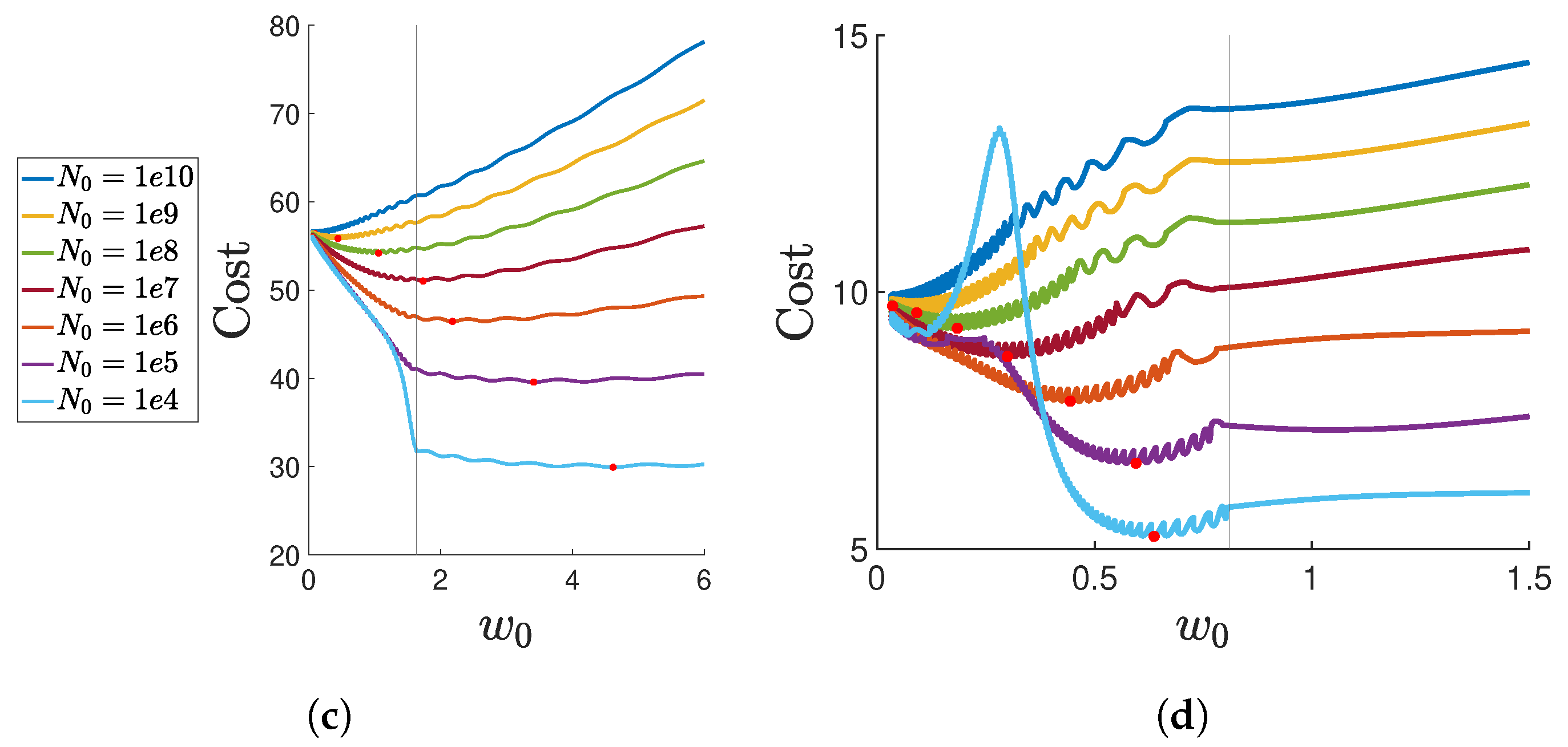
Figure A3. The cost of optimal solutions as a function of w 0 for the Gompertz model. Each panel corresponds to given values of r and d, each curve relates to a given value of N 0 , and red points represent global minima. The vertical line indicates the value of w 0 at the upper bound of the switching zone. (a) r = 1500 and d = 1.19 cells/day, (b) r = 1500 and d = 2.41 cells/day, panel (c) r = 0.1 and d = 1.19 cells/day, and (d) r = 0.1 and d = 2.41 cells/day. All illustrated trajectories relate to the following parameter values: λ = 1.865 · 10 10 cells, ε = 77,293 cells, and α = 0.95 .
Mathematics 12 03516 g0a3aMathematics 12 03516 g0a3b

Appendix F. Proof of Aperiodic Optimal Bang–Bang Solutions with Metastatic Risk

The cost functional was extended by adding into the running cost a term that is linear to the tumour size and expresses the risk of the tumour metastasising during therapy.
J = r N ( T ) + 0 T 1 α cos 2 π t u ( t ) + β N ( t ) d t
Optimal solutions were investigated for the general tumour growth model,
d N d t = f ( u ) g ( N )
where the tumour growth rate g ( N ) is positive, with 0 u u max and f ( 0 ) = 1 . The term f ( u ) is linear and strictly decreases with respect to u, satisfying d f d u = δ < 0 , δ > 0 ; i.e., the tumour growth rate falls when administering the drug. The class of tumour growth models in (A16) includes the case studied in Section 3.2, where drugs that target cell division were employed, and the natural death rate of cancer cell is fixed to zero.
We show that optimal solutions are Bang-Bang and that the optimal control is non periodic. The Hamiltonian has the following form:
H = f ( u ) g ( N ) p + 1 α cos 2 π t u ( t ) + β N ( t )
The adjoint equation is
d p d t = f ( u ) d g d N p β ,
and the switching function is given by
H u = Φ N , p , t = δ g ( N ) p + 1 α cos 2 π t .
Assuming there exists a singular solution, the order of the singular arc is determined by successively evaluating the time derivatives of the switching function.
The first derivative
d H u d t = β δ + α 2 π sin ( 2 π t ) ,
is independent of u. Then, the second derivative is evaluated:
d 2 H u d t 2 = α 4 π 2 cos ( 2 π t ) .
By enforcing the first order condition H u = 0 , equivalently, cos ( 2 π t ) = δ g ( N ) p + 1 α , we obtain,
d 2 H u d t 2 = 4 π 2 1 δ g ( N ) p ,
which is again independent of u. Then,
d 3 H u d t 3 = 4 π 2 β δ g ( N ) ,
and
d 4 H u d t 4 = 4 π 2 β δ d g d N f ( u ) g ( N ) .
Since d 4 H u d t 4 depends explicitly on u the order of the singular solution is equal to 2. The generalized LC conditions reads as follows:
( 1 ) 2 u d 4 H u d t 4 0 ,
leading to a contradiction, since u d 4 H u d t 4 = 4 π 2 β δ 2 d g d N g ( N ) < 0 (in the case where g ( N ) is zero, d N d t = 0 ); hence, the optimal solutions are Bang-Bang.
The periodicity of optimal solutions can be derived as in Section 3.1 from the form of the switching function Φ ( w , t ) = δ w + 1 α cos ( 2 π t ) by proving that w = g ( N ) p is strictly monotonic with respect to time.
Indeed, from Equation (A16), f ( u ) = 1 g ( N ) d N d t ; then, Equation (A17) reads
d w d t = β g ( N ) .
By definition g ( N ) > 0 ; hence, w ( t ) is a strictly decreasing function, and consequently optimal solutions are non-periodic, with the daily drug quantity administered decreasing as the treatment progresses.

References

  1. Ayyar, V.S.; Sukumaran, S. Circadian rhythms: Influence on physiology, pharmacology, and therapeutic interventions. J. Pharmacokinet. Pharmacodyn. 2021, 48, 321–338. [Google Scholar] [CrossRef] [PubMed]
  2. Mohawk, J.A.; Green, C.B.; Takahashi, J.S. Central and peripheral circadian clocks in mammals. Annu. Rev. Neurosci. 2012, 35, 445–462. [Google Scholar] [CrossRef] [PubMed]
  3. Farshadi, E.; van Der Horst, G.T.; Chaves, I. Molecular links between the circadian clock and the cell cycle. J. Mol. Biol. 2020, 432, 3515–3524. [Google Scholar] [CrossRef]
  4. Gérard, C.; Goldbeter, A. Entrainment of the mammalian cell cycle by the circadian clock: Modeling two coupled cellular rhythms. PLoS Comput. Biol. 2012, 8, e1002516. [Google Scholar] [CrossRef] [PubMed]
  5. Zhang, R.; Lahens, N.F.; Ballance, H.I.; Hughes, M.E.; Hogenesch, J.B. A circadian gene expression atlas in mammals: Implications for biology and medicine. Proc. Natl. Acad. Sci. USA 2014, 111, 16219–16224. [Google Scholar] [CrossRef]
  6. Feillet, C.; Krusche, P.; Tamanini, F.; Janssens, R.C.; Downey, M.J.; Martin, P.; Teboul, M.; Saito, S.; Lévi, F.A.; Bretschneider, T.; et al. Phase locking and multiple oscillating attractors for the coupled mammalian clock and cell cycle. Proc. Natl. Acad. Sci. USA 2014, 111, 9828–9833. [Google Scholar] [CrossRef]
  7. Savvidis, C.; Koutsilieris, M. Circadian rhythm disruption in cancer biology. Mol. Med. 2012, 18, 1249–1260. [Google Scholar] [CrossRef]
  8. Zhou, L.; Zhang, Z.; Nice, E.; Huang, C.; Zhang, W.; Tang, Y. Circadian rhythms and cancers: The intrinsic links and therapeutic potentials. J. Hematol. Oncol. 2022, 15, 21. [Google Scholar] [CrossRef]
  9. Lee, Y. Roles of circadian clocks in cancer pathogenesis and treatment. Exp. Mol. Med. 2021, 53, 1529–1538. [Google Scholar] [CrossRef]
  10. Tsuchiya, Y.; Ushijima, K.; Noguchi, T.; Okada, N.; Hayasaka, J.I.; Jinbu, Y.; Ando, H.; Mori, Y.; Kusama, M.; Fujimura, A. Influence of a dosing-time on toxicities induced by docetaxel, cisplatin and 5-fluorouracil in patients with oral squamous cell carcinoma; a cross-over pilot study. Chronobiol. Int. 2018, 35, 289–294. [Google Scholar] [CrossRef]
  11. Lee, Y.; Fong, S.Y.; Shon, J.; Zhang, S.L.; Brooks, R.; Lahens, N.F.; Chen, D.; Dang, C.V.; Field, J.M.; Sehgal, A. Time-of-day specificity of anticancer drugs may be mediated by circadian regulation of the cell cycle. Sci. Adv. 2021, 7, eabd2645. [Google Scholar] [CrossRef] [PubMed]
  12. Shafi, A.A.; Knudsen, K.E. Cancer and the circadian clock. Cancer Res. 2019, 79, 3806–3814. [Google Scholar] [CrossRef] [PubMed]
  13. Ballesta, A.; Innominato, P.F.; Dallmann, R.; Rand, D.A.; Lévi, F.A. Systems chronotherapeutics. Pharmacol. Rev. 2017, 69, 161–199. [Google Scholar] [CrossRef] [PubMed]
  14. Dallmann, R.; Okyar, A.; Lévi, F. Dosing-time makes the poison: Circadian regulation and pharmacotherapy. Trends Mol. Med. 2016, 22, 430–445. [Google Scholar] [CrossRef]
  15. Printezi, M.I.; Kilgallen, A.B.; Bond, M.J.G.; Štibler, U.; Putker, M.; Teske, A.J.; Cramer, M.J.; Punt, C.J.A.; Sluijter, J.P.G.; Huitema, A.D.R.; et al. Toxicity and efficacy of chronomodulated chemotherapy: A systematic review. Lancet 2022, 23, E129–E143. [Google Scholar] [CrossRef]
  16. Amiama-Roig, A.; Verdugo-Sivianes, E.M.; Carnero, A.; Blanco, J.R. Chronotherapy: Circadian Rhythms and Their Influence in Cancer Therapy. Cancers 2022, 14, 5071. [Google Scholar] [CrossRef]
  17. Squire, T.; Buchanan, G.; Rangiah, D.; Davis, I.; Yip, D.; Chua, Y.J.; Rich, T.; Elsaleh, H. Does chronomodulated radiotherapy improve pathological response in locally advanced rectal cancer? Chronobiol. Int. 2017, 34, 492–503. [Google Scholar] [CrossRef]
  18. Lévi, F.; Altinok, A.; Clairambault, J.; Goldbeter, A. Implications of circadian clocks for the rhythmic delivery of cancer therapeutics. Philos. Trans. R. Soc. A Math. Phys. Eng. Sci. 2008, 366, 3575–3598. [Google Scholar] [CrossRef]
  19. Bernard, S.; Čajavec Bernard, B.; Lévi, F.; Herzel, H. Tumor growth rate determines the timing of optimal chronomodulated treatment schedules. PLoS Comput. Biol. 2010, 6, e1000712. [Google Scholar] [CrossRef]
  20. Powathil, G.G.; Gordon, K.E.; Hill, L.A.; Chaplain, M.A.J. Modelling the effects of cell-cycle heterogeneity on the response of a solid tumour to chemotherapy Biological insights from a hybrid multiscale cellular automaton model. J. Theor. Biol. 2012, 308, 1–19. [Google Scholar] [CrossRef]
  21. Powathil, G.G.; Adamson, D.J.; Chaplain, M.A. Towards predicting the response of a solid tumour to chemotherapy and radiotherapy treatments: Clinical insights from a computational model. PLoS Comput. Biol. 2013, 9, e1003120. [Google Scholar] [CrossRef] [PubMed]
  22. Altinok, A.; Lévi, F.; Goldbeter, A. Identifying mechanisms of chronotolerance and chronoefficacy for the anticancer drugs 5-fluorouracil and oxaliplatin by computational modeling. Eur. J. Pharm. Sci. 2009, 36, 20–38. [Google Scholar] [CrossRef] [PubMed]
  23. Shi, J.; Alagoz, O.; Erenay, F.S.; Su, Q. A survey of optimization models on cancer chemotherapy treatment planning. Ann. Oper. Res. 2014, 221, 331–356. [Google Scholar] [CrossRef]
  24. Rojas, C.; Belmonte-Beitia, J. Optimal control problems for differential equations applied to tumor growth: State of the art. Appl. Math. Nonlinear Sci. 2018, 3, 375–402. [Google Scholar] [CrossRef]
  25. Jarrett, A.M.; Faghihi, D.; Hormuth, D.A.; Lima, E.A.; Virostko, J.; Biros, G.; Patt, D.; Yankeelov, T.E. Optimal control theory for personalized therapeutic regimens in oncology: Background, history, challenges, and opportunities. J. Clin. Med. 2020, 9, 1314. [Google Scholar] [CrossRef]
  26. Kuznetsov, M.; Clairambault, J.; Volpert, V. Improving cancer treatments via dynamical biophysical models. Phys. Life Rev. 2021, 39, 1–48. [Google Scholar] [CrossRef]
  27. Swan, G.W. Optimization of Human Cancer Radiotherapy; Interdisciplinary Applied Mathematics; Springer: Berlin/Heidelberg, Germany, 2015. [Google Scholar]
  28. Martin, R.; Te, K.L. Optimal Control of Drug Administration in Cancer Chemotherapy; World Scientific Publishing Company Pte. Ltd.: Singapore, 1994. [Google Scholar] [CrossRef]
  29. Schattler, H.; Ledzewicz, U. Optimal Control for Mathematical Models of Cancer Therapies an Application of Geometric Methods; Lecture Notes in Biomathematics v 42; Springer: Berlin/Heidelberg, Germany, 2015. [Google Scholar]
  30. Dömény, M.F.; Puskás, M.; Kovács, L.; Drexler, D.A. A Review of Multi-Objective Optimization Algorithms in the Field of Chemotherapy Optimization. In Proceedings of the 2024 IEEE 18th International Symposium on Applied Computational Intelligence and Informatics (SACI), Siófok, Hungary, 21–25 May 2024; pp. 345–350. [Google Scholar]
  31. Barbolosi, D.; Iliadis, A. Optimizing drug regimens in cancer chemotherapy: A simulation study using a PK–PD model. Comput. Biol. Med. 2001, 31, 157–172. [Google Scholar] [CrossRef]
  32. Ballesta, A.; Dulong, S.; Abbara, C.; Cohen, B.; Okyar, A.; Clairambault, J.; Levi, F. A combined experimental and mathematical approach for molecular-based optimization of irinotecan circadian delivery. PLoS Comput. Biol. 2011, 7, e1002143. [Google Scholar] [CrossRef]
  33. Basdevant, C.; Clairambault, J.; Lévi, F. Optimisation of time-scheduled regimen for anti-cancer drug infusion. Esaim Math. Model. Numer. Anal.—Modélisation Mathématique et Analyse Numérique 2005, 39, 1069–1086. [Google Scholar] [CrossRef]
  34. Clairambault, J.; Fercoq, O. Physiologically structured cell population dynamic models with applications to combined drug delivery optimisation in oncology. Math. Model. Nat. Phenom. 2016, 11, 45–70. [Google Scholar] [CrossRef]
  35. Angaroni, F.; Graudenzi, A.; Rossignolo, M.; Maspero, D.; Calarco, T.; Piazza, R.; Montangero, S.; Antoniotti, M. An optimal control framework for the automated design of personalized cancer treatments. Front. Bioeng. Biotechnol. 2020, 8, 523. [Google Scholar] [CrossRef] [PubMed]
  36. Gamkrelidze, R. Selected Research Papers: L. S. Pontryagin Select Works; CRC Press: Boca Raton, FL, USA, 2019; Volume 1. [Google Scholar]
  37. Locatelli, A. Optimal Control: An Introduction; Springer Science & Business Media: Berlin/Heidelberg, Germany, 2001. [Google Scholar]
  38. Robbins, H. A generalized Legendre-Clebsch condition for the singular cases of optimal control. IBM J. Res. Dev. 1967, 11, 361–372. [Google Scholar] [CrossRef]
  39. Rao, A.V. A survey of numerical methods for optimal control. Adv. Astronaut. Sci. 2009, 135, 497–528. [Google Scholar]
  40. Crozier, L.; Foy, R.; Adib, R.; Kar, A.; Holt, J.A.; Pareri, A.U.; Valverde, J.M.; Rivera, R.; Weston, W.A.; Wilson, R.; et al. CDK4/6 inhibitor-mediated cell overgrowth triggers osmotic and replication stress to promote senescence. Mol. Cell 2023, 83, 4062–4077.e5. [Google Scholar] [CrossRef]
  41. Murphy, H.; Jaafari, H.; Dobrovolny, H.M. Differences in predictions of ODE models of tumor growth: A cautionary example. BMC Cancer 2016, 16, 163. [Google Scholar] [CrossRef]
  42. Benzekry, S.; Lamont, C.; Beheshti, A.; Tracz, A.; Ebos, J.M.; Hlatky, L.; Hahnfeldt, P. Classical mathematical models for description and prediction of experimental tumor growth. PLoS Comput. Biol. 2014, 10, e1003800. [Google Scholar] [CrossRef]
  43. Kimmel, M.; Swierniak, A. Control Theory Approach to Cancer Chemotherapy: Benefiting from Phase Dependence. Lect. Notes Math. 2006, 1872, 185–221. [Google Scholar]
  44. Ledzewicz, U.; Bratton, K.; Schattler, H. A 3-Compartment Model for Chemotherapy of Heterogeneous Tumor Populations. Acta Appl. Math. 2015, 135, 191–207. [Google Scholar] [CrossRef]
  45. Ledzewicz, U.; Schättler, H. Optimal bang–bang controls for a two-compartment model in cancer chemotherapy. J. Optim. Theory Appl. 2002, 114, 609–637. [Google Scholar] [CrossRef]
  46. Faivre, C.; Barbolosi, D.; Pasquier, E.; André, N. A mathematical model for the administration of temozolomide: Comparative analysis of conventional and metronomic chemotherapy regimens. Cancer Chemother. Pharmacol. 2013, 71, 1013–1019. [Google Scholar] [CrossRef]
  47. Basse, B.; Ubezio, P. A generalised age-and phase-structured model of human tumour cell populations both unperturbed and exposed to a range of cancer therapies. Bull. Math. Biol. 2007, 69, 1673–1690. [Google Scholar] [CrossRef] [PubMed]
  48. Swierniak, A.; Ledzewicz, U.; Schättler, H. Optimal control for a class of compartmental models in cancer chemotherapy. Int. J. Appl. Math. Comput. Sci. 2003, 13, 357–368. [Google Scholar]
  49. Michor, F.; Beal, K. Improving Cancer Treatment via Mathematical Modeling: Surmounting the Challenges Is Worth the Effort. Cell 2015, 163, 1059–1063. [Google Scholar] [CrossRef] [PubMed]
  50. Magi, S.; Iwamoto, K.; Okada-Hatakeyama, M. Current status of mathematical modeling of cancer â From the viewpoint of cancer hallmarks. Regulatory and metabolic networks ⢠Cancer and systemic diseases. Curr. Opin. Syst. Biol. 2017, 2, 39–48. [Google Scholar] [CrossRef]
  51. Jarrett, A.M.; Lima, E.A.B.F.; Hormuth, D.A.n.; McKenna, M.T.; Feng, X.; Ekrut, D.A.; Resende, A.C.M.; Brock, A.; Yankeelov, T.E. Mathematical models of tumor cell proliferation: A review of the literature. Expert Rev. Anticancer. Ther. 2018, 18, 1271–1286. [Google Scholar] [CrossRef]
  52. Bekisz, S.; Geris, L. Cancer modeling: From mechanistic to data-driven approaches, and from fundamental insights to clinical applications. J. Comput. Sci. 2020, 46, 101198. [Google Scholar] [CrossRef]
  53. Yin, A.; Moes, D.J.A.; van Hasselt, J.G.; Swen, J.J.; Guchelaar, H.J. A review of mathematical models for tumor dynamics and treatment resistance evolution of solid tumors. CPT Pharmacomet. Syst. Pharmacol. 2019, 8, 720–737. [Google Scholar] [CrossRef]
  54. Hill, R.J.; Innominato, P.F.; Lévi, F.; Ballesta, A. Optimizing circadian drug infusion schedules towards personalized cancer chronotherapy. PLoS Comput. Biol. 2020, 16, e1007218. [Google Scholar] [CrossRef]
  55. Clairambault, J. Modeling oxaliplatin drug delivery to circadian rhythms in drug metabolism and host tolerance. Adv. Drug Deliv. Rev. 2007, 59, 1054–1068. [Google Scholar] [CrossRef]
  56. Borzì, A.; Schulz, V. Multigrid Methods for PDE Optimization. SIAM Rev. 2009, 51, 361–395. [Google Scholar] [CrossRef]
  57. Bensoussan, A.; Da Prato, G.; Delfour, M.C.; Mitter, S. (Eds.) Representation and Control of Infinite Dimensional Systems, 2nd ed.; Birkhauser: Boston, MA, USA, 2007. [Google Scholar]
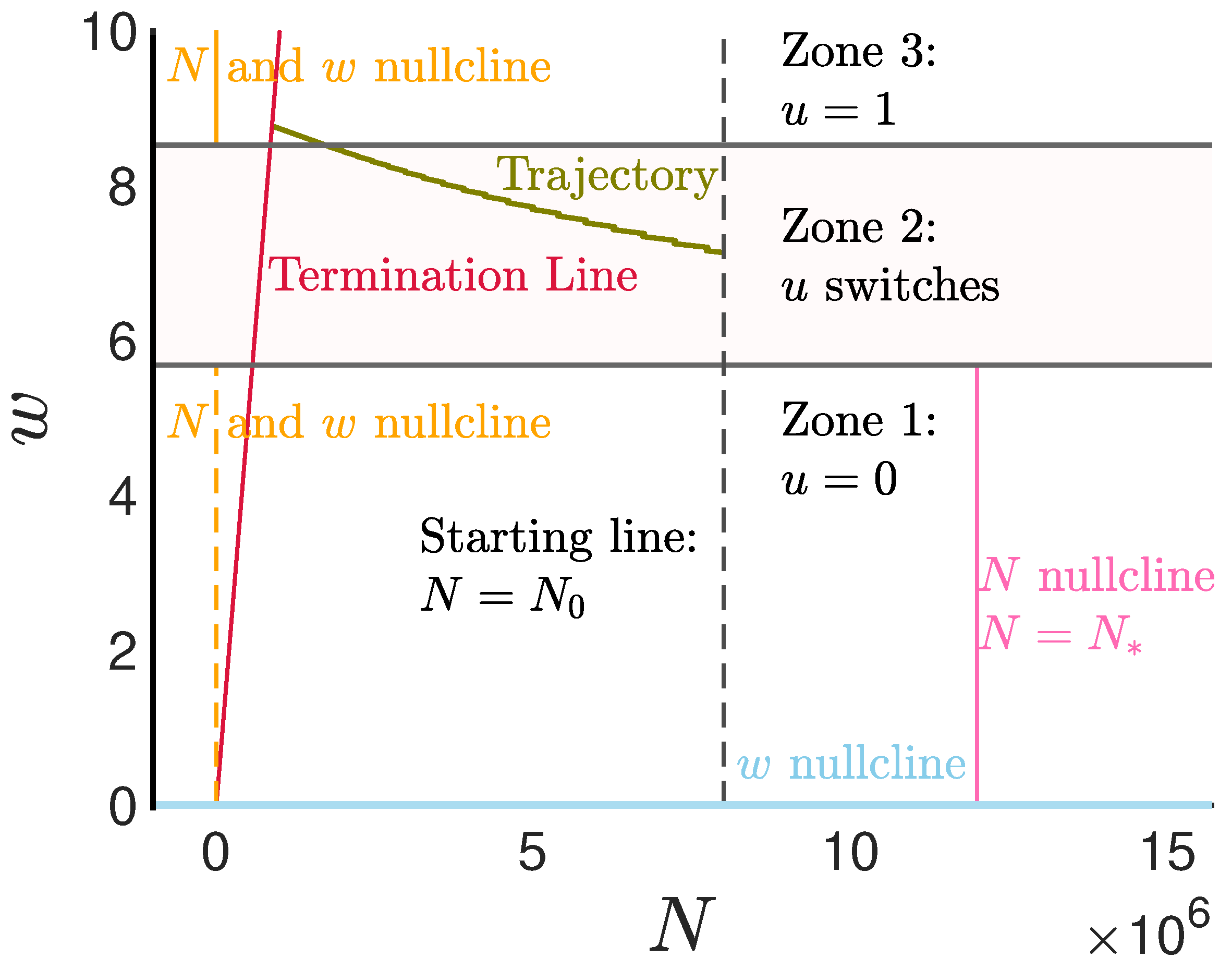
Figure 1. Graphical representation of trajectory dynamics, which are admissible under PMP, in the N w plane. Trajectories start on the initialisation line (tumour size N = N 0 ), i.e., the black dashed vertical line, and end on the termination line w = r N , (red line). The N w plane is divided into three zones: zone 1 ( w < min ( h ) ), with u = 0 ; zone 2 ( min ( h ) w < max ( h ) ), the switching zone, where u is either 0 or 1; and zone 3 ( w max ( h ) ), with u = 1 . Finally, the nullclines are shown (region dependent), with w-nullcline w = 0 in blue, N-nullclines N = 0 in orange, and N = N * in magenta. In zone 1, the orange vertical line N = 0 is both a w and N nullcline. A trajectory is illustrated in green starting from N = N 0 (the dashed black line) and terminating when it reaches the (red) termination line w = r N . Trajectories can only occur in the upper quadrant. Sketch is based on the Gompertz model with a carrying capacity of N * = 8 · 10 6 cells.
Mathematics 12 03516 g001
Figure 2. Trajectory solutions in the N w plane for the logistic model. There are 3 cases depending on the initial tumours: (a) large initial tumour size, N 0 > N b ; (b) intermediate initial tumours, N b > N 0 > N a ; (c) small initial tumours N 0 < N a . Trajectories are colour coded by type, classified in Figure 3. The switching zone boundaries, w = 1 α d and w = 1 + α d , are indicated by black horizontal lines. The vertical solid lines ( N = N a and N = N b ) indicate the intersection of the termination line with the lower and upper switching bounds, respectively. Each trajectory starts on the intialisation line ( N = N 0 ), the black dashed one, and terminates on the termination line ( w = r N ), shown in thick black lines. Grey arrows represent the flow of solutions in zones 1 and 3 respectively. Parameter values are λ = 0.0625 per day, d = 0.125 per day, r = 50 · 10 8 days per cell, K = 10 8 cells, and α = 0.1 .
Mathematics 12 03516 g002
Figure 3. Classification of solutions in the N w plane for the logistic model for large tumours (case A, N 0 > N b ). The switching zone boundaries are indicated by horizontal black lines. Possible trajectories start on the initialisation line (dashed, N = N 0 ) and terminate on the termination line (thick black line lying close to the w-axis). Trajectories are classified as follows: Type-0 (brown) starts in zone 1, traverses across zone 2, and ends in zone 3; the tumor size increases until the switching zone is reached, where the trajectories drift towards the termination line, reaching termination only under continuous MTD in zone 3. Type-1 (red) trajectories are similar to Type-0 but start in zone 1 and traverse to and end in zone 2; the tumor size increases until the switching zone is reached, where the trajectories drift towards the termination line. Type-2 (blue) trajectories start and end in zone 2, with N increasing beyond N 0 (there exists s [ 0 , T ] s.t. N ( s ) > N 0 ); despite starting in the switching zone with daily drug administration, these trajectories take a “detour“ away from the termination line to larger tumour sizes. Type-3 trajectories (black) start and end in zone-2, with the tumor size always less than N 0 ; these trajectories are the most cost-efficient, with daily switching reducing drug toxicity, and a low final tumor size can be attained. Type-4 (purple) trajectories start in zone-2 and end in zone-3; they are similar to type-3 trajectories except they shift to continuous MTD at the end of treatment;. Type-5 (orange) trajectories start and end in zone-3; MTD is applied continuously, and the terminal tumor size approaches N 0 as T 0 . Parameter values: α = 0.07 , K = 10 8 cells, r = 5000 · 10 8 days per cell, d = 0.125 per day, and λ = 0.025 per day. Parameter values were chosen to illustrate the types of optimal solutions.
Mathematics 12 03516 g003
Figure 4. Daily drug infusion and tumour decay for a type 3 solution to the logistic model. (a) Classification of solutions (colour coding by type as in Figure 3); there is no type 0 for these parameter values and the initial tumour size. (b) Daily drug administration duration (hours). (c) Daily relative reduction in tumor size (relative to the beginning of the day) throughout the treatment. The parameter values are the same as in Figure 3 except for α = 0.3 , with an initial tumor size of N 0 = 10 7 cells. Time horizon is T = 45 days in panels (b,c).
Mathematics 12 03516 g004
Figure 5. Logistic model solution costs and time horizons. (a) The dependence of the time horizon, (b) total cost, (c) terminal cost, and (d) running cost on the initial value of w 0 . Solution types are colour-coded as in Figure 3. The inset plots in panels (a,b) show the time horizon and cost as a function of w 0 for Type-5 solutions. The initial tumor size and parameter values are given as in Figure 4.
Mathematics 12 03516 g005
Figure 6. Details of cost and time horizon dependence on w 0 for the logistic model. (a) The cost and (b) the time horizon for a narrow region of w 0 values around the global minimum cost solution. The parameter values and the initial tumour size are the same as those in Figure 4.
Mathematics 12 03516 g006
Figure 7. Details of w ( t ) as termination is approached for 3 solutions with close w 0 values (logistic model). The 3 cases correspond to (a) w 0 = 9.2410 that terminates just before the next switching time, (b) w 0 = 9.2364 that terminates at the switching time, and (c) that reaches the termination line and terminates just after a switching event. Switching and termination points are represented with red and black marks, respectively, thick black line is the trajectory w ( t ) and thin black curves are the function h ( t ) . The areas of the w t plane where w ( t ) < h ( t ) and w ( t ) > h ( t ) are coloured white and pink, respectively. All trajectories reach the termination line when w ( T ) h ( T ) , resulting in a discontinuity in the time horizon as w 0 decreases past w 0 = 9.2364 (case (b)). Parameter values and the initial tumour size are the same as in Figure 4.
Mathematics 12 03516 g007aMathematics 12 03516 g007b
Figure 8. Construction of solutions with multiple termination line crossings (logistic model). (a) A segment of a trajectory in the N w plane that intersects the termination line three times. Trajectory components are colour coded, before the first crossing of the termination line (black), after first crossing and before second (orange), after second crossing (green). Termination line is shown (black) and crossings indicated by dots coloured as the prior trajectory segment. Switching points are shown (red). Trajectory starts at N 0 = 0.1 · 10 8 , w 0 = 5.699 and can terminate on the first, second or third crossing giving 3 horizon times for that w 0 . (b) The time horizon as a function of w 0 over range 7.2 w 0 7.3 . Points that correspond to trajectories that cross the termination line once, twice and three times are coloured in black, orange and green respectively. The parameter values and the initial tumour size are the same as those in Figure 4.
Mathematics 12 03516 g008
Figure 9. The cost for trajectories that cross the termination line up to three times in the logistic model. (a) The dependence of the cost on w 0 , in a region where the cost takes its minimum value. (b) The cost of the same solutions as in (a) shown as a function of the time horizon, T. Trajectories are coloured by number of crossings—1 black, 2 orange, and 3 green. The parameter values and the initial tumour size are the same as in Figure 4.
Mathematics 12 03516 g009
Figure 10. Gompertz model solution costs and time horizons. (a) The dependence of the time horizon, (b) total cost, (c) terminal cost, and (d) running cost on the initial value of w 0 . Colours correspond to the solution type classification in Figure 3. The inset plots in panels (a,b) show the time horizon and cost as a function of w 0 for type-5 solutions. Parameter values: ε λ = 1 3 , g = 0.025 per day, d = 0.1373 , per day r = 5000 · 10 8 days per cell, and α = 0.3 . The initial tumor size is N 0 = 0.1 · 10 8 cells. Parameter values were selected to illustrate behaviour of the optimal solutions.
Mathematics 12 03516 g010aMathematics 12 03516 g010b
Figure 11. Cost of multiple termination-line-crossing solutions for the Gompertz model. (a) The dependence of the cost on w 0 shown over the range 6.49 w 0 6.52 . Termination points that correspond to trajectories that satisfy the transversality condition at the first, second, or third crossing of the termination line are coloured in black, orange, and green, respectively. (b) The terminal value w ( T ) against the time horizon for trajectories in panel (a). The control value upon termination, u ( T ) , is shown by background shading; pink area is u ( T ) = 1 ; and white area is u ( T ) = 0 . Termination points coloured as in panel (a). The parameters and the initial tumour size are the same as in Figure 10.
Mathematics 12 03516 g011
Figure 12. Switching function and drug scheduling for a solution satisfying PMP. (a) The switching function Φ ( t ) ; green and red colors illustrate time periods where the control u is 1 and 0, respectively. The inset plot shows Φ ( t ) for the first 41 days of therapy. (b) the percentage of each day in which a drug is administered; orange bars relate to days in which the drug is chronomodulated, blue bars relate to days wherein MTD is administered continuously, and the horizontal line shows the respective percentage of the optimised periodic drug regimen. The inset plot illustrates the percentage for the first 41 days of therapy. The time horizon is 1 year, the number of dividing ( N 1 ) and non-dividing ( N 2 ) cancer cells at t = 0 are N 1 ( 0 ) = 6.4376 · 10 7 and N 2 ( 0 ) = 3.5624 · 10 7 ; the growth rates of dividing and non-dividing cancer cells are a 1 = 0.1970 and a 2 = 0.3560 , respectively. The parameters that weight the terminal tumour size in the cost function are r 1 = 52.5339 and r 2 = 31.2068 .
Mathematics 12 03516 g012
Figure 13. Tumour size for the PMPDR solution: (a) Number of dividing cancer cells ( N 1 ) as a function of time, (b) number of non-dividing cancer cells ( N 2 ) as a function of time. The inset plots in (a,b) show details of the time evolution of N 1 and N 2 , respectively.
Mathematics 12 03516 g013
Figure 14. Example trajectories for a tumour with low ( d = 1.19 per day, panels (a,b)) and high ( d = 2.41 per day, panels (c,d)) susceptibility to the drug. Tumour evolution was assumed to be Gompertzian. (a,c) N as a function of time, and (b,d) w (dashed line) as a function of time. The periodic switching threshold h ( t ) is shown in blue and the upper bound of the switching zone in black. N ( t ) and w ( t ) at switching and termination points are shown as black and red dots respectively. The inset panels show the time evolution of N and w over a longer time period. Parameters are g = 0.0792 per day, r = 1500 days/cell, α = 0.95 , ε = 77,293 cells, and λ = 1.865 × 10 10 cells, and the drug-induced death rates are d = 1.19 , and 2.41 per day for panels (a,b) and (c,d), respectively. Initial tumour size is 10 8 cells.
Mathematics 12 03516 g014
Figure 15. Comparison of (unconstrained) optimal solutions (in light red) and optimal solutions constrained to be periodic (in black) for tumours with low susceptibility to the drug (Gompertz model). (a) Terminal tumour size versus N 0 , (b) toxicity to normal cells (running cost) versus N 0 , (c) treatment duration versus N 0 , (d) total drug quantity administered versus N 0 , (e) the fractional administration time versus N 0 , and (f) percentage reduction of the running cost of unconstrained compared to constrained optimal solutions. Model parameters are the same as in Figure 14, with d = 1.19 per day.
Mathematics 12 03516 g015
Figure 16. Comparison of (unconstrained) optimal solutions (in light red), optimal constrained (periodic) solutions (asterisks), and continuous MTD (square) for tumours with high drug susceptibility (Gompertz model). (a) Terminal tumour size versus N 0 , (b) toxicity to normal cells (running cost) versus N 0 , (c) treatment duration versus N 0 , (d) total drug administered versus N 0 , (e) the fractional administration time versus N 0 , and (f) percentage reduction of the running cost of specified treatments versus N 0 . Model parameters as Figure 14, d = 2.41 per day.
Mathematics 12 03516 g016
Disclaimer/Publisher’s Note: The statements, opinions and data contained in all publications are solely those of the individual author(s) and contributor(s) and not of MDPI and/or the editor(s). MDPI and/or the editor(s) disclaim responsibility for any injury to people or property resulting from any ideas, methods, instructions or products referred to in the content.